Transmit-Receive Generalized Spatial Modulation Based on Dual-layered MIMO Transmission
Abstract
We propose a novel scheme for downlink multiuser MIMO (MIMO) systems, called DL-TR-GSM (DL-TR-GSM). The proposed scheme is based on the concept of DLT (DLT) which uses two receive antenna power levels instead of receive antenna activation/inactivation to transmit data in the receive spatial domain. Hence, in order to minimize the BER (BER) for DL-TR-GSM, the optimal ratio between the two power levels is determined. To further characterize DL-TR-GSM, we fully derive the computational complexity and show a significant computational complexity reduction as well as a required hardware complexity reduction of DL-TR-GSM, compared to a state-of-the-art benchmark scheme. Simulation results confirm the performance advantages of DL-TR-GSM.
Index Terms:
Dual-layered transmission, GSM (GSM), MIMO, multiuser communications.I Introduction
Among many existing MIMO schemes, SM (SM) has attracted a lot of research interest in recent years. In SM, two data streams are transmitted — one in the conventional IQ (IQ) domain (by employing e.g. PSK or QAM modulation), and the other in the so-called spatial domain by selecting and activating one from all available transmit antenna [1, 2]. A straightforward extension of SM is to allow activation of more than one transmit antennas per time slot and possibly also to transmit more than one IQ stream simultaneously [3]. The extended scheme is called GSM.
Recently, a scheme which is operationally dual to SM was developed, called RSM (RSM) [4, 5]. The main difference between SM and RSM comes from the signal transmission in the spatial domain, where RSM transmits data by selecting one out of all available receive antennas. Accordingly, this antenna is used for the reception of the transmitted IQ stream. Similarly, the concept of RSM may be extended by selecting more than one receive antenna per time slot for the reception of multiple IQ stream transmission [6, 7]. This scheme is called GRSM (GRSM).
Another interesting extension of RSM is that of DLT [8]. In contrast to conventional RSM/GRSM which utilizes a subset of the receive antennas, DLT uses all available receive antennas for the reception of the transmitted IQ streams. Consequently, DLT requires a new approach to transmit information in the spatial domain and thus DLT applies two power levels to distinguish the “selected” from the “non-selected” receive antennas in the spatial domain [8]. In this way, the spatial symbols are encoded onto the signal power levels at the receive antennas.
Although the basic theory for SM and RSM was initially developed for single-user communication systems, an increasing number of research works consider their application in multiuser scenarios. In [9], the authors considered a multiuser uplink transmission scheme with SM implemented at each user. To enable SM in multiuser downlink communications, a closed-form precoding solution was derived in [10]. In [11], an implementation of RSM/GRSM in massive MIMO systems was investigated. A more detailed analysis of GRSM for multiuser downlink communications was presented in [12].
The papers listed above consider multiuser communication schemes that are based on the SM or the RSM operation principle. To the best of the authors’ knowledge, the only multiuser scheme that simultaneously supports the SM and RSM operation principle is presented in [13], and is called MU-TR-GSM (MU-TR-GSM). In each time slot, the base station in MU-TR-GSM selects a subset of the transmit antennas to be active. From those antennas, the base station transmits IQ streams to the users. Also, this antenna activation enables MU-TR-GSM to send data in the transmit spatial domain. Each user receives the transmitted IQ streams by a subset of receive antennas, whose selection enables MU-TR-GSM to send data in the receive spatial domain. Therefore, MU-TR-GSM manages to combine the principles of operation of SM and RSM. Despite the advantage of combining the SM and the RSM operation principles, MU-TR-GSM requires a high computational complexity (see Section Subsection IV-A) which presents a significant barrier to its practical implementation.
Against this background, the contributions of this paper are listed as follows:
- 1.
We propose a novel multiuser communication scheme, called DL-TR-GSM, that simultaneously supports the operation of the SM and RSM operation principles. However, in contrast to MU-TR-GSM which applies the conventional RSM transmission, DL-TR-GSM is based on DLT.
- 2.
We show, through a detailed computational complexity analysis and through simulations, that DL-TR-GSM enables a considerable computational complexity reduction, at the cost of a minor degradation in the BER performance.
- 3.
We also provide a hardware complexity analysis which demonstrates that DL-TR-GSM requires a lower number of RF chains at the receiver compared to MU-TR-GSM. As a result, DL-TR-GSM provides a large reduction of the receive power consumption at each user.
- 4.
We introduce a low-complexity detector for DL-TR-GSM, referred to as the separate detector. Simulation results show that this detector provides a very similar BER to that provided by the optimal ML (ML) detector.
II System Model
II-A DL-TR-GSM
The block diagram for the considered DL-TR-GSM scheme is shown in Fig. 1. It depicts a downlink communication scenario between a base station equipped with transmit antennas and users equipped with receive antennas per user. Accordingly, the channel matrix of the DL-TR-GSM scheme can be expressed as
where is the channel matrix between the base station and the -th user.
In each time slot, the base station activates a subset of () transmit antennas, which form 1 out of transmit antenna combinations. For ease of comparison of our later results with those in [13], we assume that each transmit antenna can belong to only one transmit antenna combination; thus, the data rate in the transmit spatial domain is instead of . For the s-th combination of activated transmit antennas (), the resulting channel matrix consists of the columns of that correspond to the active transmit antennas. Implementing SVD (SVD) on any constituent matrix of , we obtain
| (1) |
where is a unitary matrix, is a diagonal matrix of singular values and . Now, the overall receive signal vector of all users, , can be written as [14]
| (2) |
where, according to (1), we introduced the definitions
Moreover, is the transmit signal vector of the base station and is the noise vector with iid (iid) elements that are distributed according to , where denotes the (one-sided) power spectral density of the additive white Gaussian noise (AWGN).
To enable downlink signal transmission without inter-channel and inter-user interference, a precoder is required at the transmitter. Hence, the transmit IQ symbol vector , which contains IQ symbols of the M-PSK modulation alphabet, is precoded before its transmission, yielding the vector

The precoding matrix is defined as
| (3) |
where the diagonal matrix serves to ensure a constant average transmit power. Assuming that all diagonal elements in are equal as in [14], we obtain , where
| (4) |
In the remainder of the paper, we will assume that this is the case, and we will refer to as the scaling coefficient.
To transmit data in the receive spatial domain, DL-TR-GSM utilizes the power level matrix . Each constituent matrix () is a diagonal matrix whose -th diagonal element takes the value if the -th receive antenna of the k-th user is “non-selected” or if the -th receive antenna of the k-th user is “selected”. Indices of the “selected” and the “non-selected” receive antennas of one user determine bits transmitted to that user in the receive spatial domain. More precisely, the indices of the “non-selected” receive antennas specify the positions of zeros and the indices of the “selected” receive antennas specify the positions of ones. Hereinafter, we assume and the set of all possible is denoted by (hence ).
From the previous expressions, the receive signal vector of the -th user can be written as follows:
| (5) |
where and are the index of the transmitted IQ symbol vector and the index of the used power level matrix for the -th user, respectively. To cover the data transmission in all three domains we refer to the column vector as the supersymbol, where . One should note that each supersymbol is uniquely determined by a particular index combination.
Now, the optimal ML detector of the k-th user is given as
| (6) |
where is the index of the detected transmit antenna combination, is index of the detected power level matrix and is the index of the detected IQ modulation symbol vector.
Finally, we may note that the data rate per user of DL-TR-GSM is
| (7) |
II-B MU-TR-GSM
As mentioned previously, the main difference between MU-TR-GSM and DL-TR-GSM is the data transmission in the receive spatial domain. In contrast to DL-TR-GSM which uses the DLT, MU-TR-GSM follows the conventional RSM operation principle. It selects a subset of receive antennas at one user, so that each active receive antenna in the subset receives one IQ stream. Since there are receive antenna combinations, the data rate in the receive spatial domain is bits per user. Another consequence of this change is the construction of the effective channel matrix . Here, is obtained by selecting columns and rows of that correspond to the active transmit and receive antennas, respectively. Further signal preprocesing at the transmitter is same as for DL-TR-GSM. The only difference is that the precoding matrix expression does not contain the power level matrix and that the ratio numerator in (4) should be replaced by . At the reception, we execute the ML detection as explained in [13].
III Determining the Optimum Power Levels
In this section, we derive the BEP (BEP) expression for DL-TR-GSM and based on this we derive the optimal power levels and . As all the users are assumed to have the same propagation conditions, the following analytical development is user-independent. Therefore, the following expressions are valid for an arbitrary user and we omit the user index in the superscript.
The upper bound for the BEP is given by [15]
| (8) |
where the indices and determine, respectively, the transmitted and the detected supersymbol. denotes the average PEP (PEP) between the aforementioned mentioned supersymbols and is the Hamming distance between the binary representations of these supersymbols. For a given , if the ML detection in (6) is used, the PEP can be expressed as
Since the left-hand side in the previous equation is distributed according to , we get
| (9) |
where is the Euclidean distance between the considered supersymbols.
III-A Power Ratio
The ratio of the power levels used for communicating data in the receive spatial domain is
| (10) |
and it satisfies . While the chosen power levels need to maintain the average transmit power unchanged, we have Thus we obtain and Since and are determined entirely by , the goal is to find the optimal that ensures the best error rate performance.
Note that while (9) captures the PEPs associated with all possible error events for DL-TR-GSM, for mathematical tractability reasons we will consider in the following analysis only the individual PEPs of the IQ domain and of the receive spatial domain. In these two cases, the Euclidean distance of DL-TR-GSM in (9) is mathematically equivalent to the Euclidean distance of a transmit system that consists of parallel orthogonal subchannels. As the channel gains of these subchannels are proportional to the singular values in , the minimum Euclidean distances, i.e. the maximum PEP, will always occur in the subchannel with the channel gain proportional to the smallest singular value .
In the IQ domain, due to the use of M-PSK modulation, the maximum PEP can be expressed as follows:
| (11) |
For two M-PSK symbols and , we have and the previous expression can be re-written as
| (12) |
From (9), the maximum PEP of the receive spatial domain is given as
| (13) |
IV System Complexity Analysis
IV-A Computational Complexity
In this subsection, we derive the computational complexity of DL-TR-GSM and MU-TR-GSM. The computational complexity refers to the number of mathematical operations required for the calculation of all SVD and scaling coefficients that are needed in order to perform signal transmission and detection.
In DL-TR-GSM, SVD is performed for matrices of dimension , and operations are needed for each SVD [16]. As SVDs are required for each user, the total number of all SVD in DL-TR-GSM equals . The complexity of computing is primarily determined by the complexity of the denominator in (4). Since the matrix is a Hermitian matrix, only the elements on the main diagonal and below (or above), i.e. matrix elements, need to be computed. Since the computation of a single element requires operations, the computational complexity of is . Inversion of the aforementioned matrix requires operations [17] and the computation of the matrix trace requires operations. In addition, we have 1 square root, 1 multiplication and 1 division operation. The number of different values in DL-TR-GSM is . In summary, the total computational complexity of DL-TR-GSM is given by
The computational complexity derivation given above for DL-TR-GSM is applicable with some minor modifications to MU-TR-GSM. One difference comes from the fact that the MU-TR-GSM scheme activates out of available receive antennas. The other difference originates from the number of SVD and values which are given by and respectively for MU-TR-GSM. To summarize, the computational complexity of MU-TR-GSM is given by
IV-B Hardware Complexity
The fact that the transmitted IQ streams are received by all the receive antennas, and not by some receive antenna subset, enables DL-TR-GSM to use a smaller number of receive antennas compared to MU-TR-GSM. As the number of receive antennas corresponds to the number of RF chains at the receiver in RSM-based systems, the hardware complexity advantage of DL-TR-GSM becomes apparent. Consequently, we can illustrate it in terms of the receive power consumption. In the following, the receive power consumption is expressed relative to the low noise amplifier power , the RF chain power , the analog-to-digital converter power and the baseband power . The receive power consumption for both schemes may be computed as
The component powers are expressed relative to the reference power as , and [18]. For the reception of 2 IQ streams per user, under the same data rate, DL-TR-GSM requires receive antennas, and MU-TR-GSM requires receive antennas from which receive antennas are always active. If [18], the receive power consumption for DL-TR-GSM and MU-TR-GSM are 720 mW and 1240 mW, respectively. Hence, DL-TR-GSM requires 520 mW less power per user, corresponding to a 41.9 % reduction compared to MU-TR-GSM. These power gains may provide remarkable power savings, especially for communication systems supporting a large number of users.
V Separate Detector
Due to limited hardware and software resources in user terminals, a direct implementation of the ML detector in (6) may be unsuitable for practical use. Motivated by this fact, we propose a low-complexity separate detector, which executes a two-step detection process.
In the first step, the separate detector determines the most likely transmit IQ symbol vector and power level matrix for each transmit antenna combination. Assuming that the -th transmit antenna combination is activated, we perform the following signal processing at the receiver utilizing as
For (i.e. ), this system of equations corresponds to a set of parallel subchannels. Hence, we can detect the power level and the transmission symbol independently for each receive antenna as
| (15) |
Now for each transmit antenna combination we have the candidate power level matrix and the candidate transmitted IQ symbol vector .
VI Simulation Results
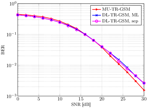
In this section, we present the BER simulation results of DL-TR-GSM with the ML detector and the separate detector. As a benchmark, we use MU-TR-GSM for performance comparison. Then we show the influence of the power ratio on the BER of DL-TR-GSM. Finally, we provide a comparison of the computational complexity of DL-TR-GSM and MU-TR-GSM.
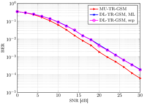
We consider a downlink communication system with a single base station and users. The base station has available transmit antennas and always activates transmit antennas. Each user receives 2 IQ streams of QPSK symbols. To maintain the same data rate, each user in DL-TR-GSM is equipped with receive antennas, while in MU-TR-GSM each user is equipped with receive antennas from which receive antennas are always used for the IQ stream reception.
In Fig. 2, we show the BER of DL-TR-GSM and MU-TR-GSM without utilizing the scaling coefficient (i.e., setting ). Due to omitting the scaling coefficient, the precoder cannot maintain the same average signal power at the input and the output. Hence this performance comparison cannot be considered as generally fair, but we present it in order to show that the BER performance matches with the results in [13, Fig. 2]. In this case we define the SNR (SNR) as the ratio of the signal power at the precoder input and the noise power. This differs from the standard way of defining the SNR as the ratio of the signal power at the transmit/receive antennas and the noise power. In general, DL-TR-GSM achieves worse BER than MU-TR-GSM and this effect becomes more pronounced at higher SNR. Accordingly, MU-TR-GSM exhibits up to 3 dB lower BER than DL-TR-GSM at high SNR. On the other hand, both schemes have the same BER in the low-SNR regime. As for the separate detector of DL-TR-GSM, we see that it exhibits no performance loss with respect to the optimal ML detector.
As already mentioned, omitting the scaling coefficient the precoders of the considered schemes are not able to maintain the same average signal power and the BER comparison in Fig. 2 cannot be classified as fair. Motivated by this, we present in Fig. 3 the BER of DL-TR-GSM and MU-TR-GSM when the scaling coefficient is utilized. In this case, the DL-TR-GSM shows a negligibly worse BER performance than MU-TR-GSM. Actually, the only visible difference is in the high-SNR regime. On the other hand, DL-TR-GSM can even achieve slightly better results at low SNR. Again, the BER of DL-TR-GSM remains extremely similar for the ML detector and the separate detector.

To evaluate the correctness of the derived expression (14), we show the BER of DL-TR-GSM as a function of the power ratio in Fig. 4. The setup and parameters are the same as in the previous figures, and the only difference is that the IQ modulation order is allowed to vary. For the used IQ modulation orders of 4, 8 and 16, the optimal values of in (14) are 5.83, 3.12 and 1.93, respectively. These values are presented with dashed lines in Fig. 4. In all cases the optimal in (14) provides a BER which is very close to the minimum achievable as shown by the simulations in Fig. 4. Also, it can be observed that the BER is very robust to the change of for low IQ modulation orders (e.g., ).

In Fig. 5, we show the BER of DL-TR-GSM for different numbers of users. Here we consider a number of users equal to 2, 4 and 8, and we assume for each value of that the number of active transmit antennas is (assuming two receive antennas per user). Also, to maintain the same data rate in the transmit spatial domain as increases, we assume that the base station is equipped with transmit antennas. It can be seen that the BER increases slightly with increasing , but this trend exhibits saturation at moderate values of . Therefore, in a system with many users, a minor variation in the number of users has a negligible impact on the system’s BER performance. Also, a good match is again observed between the BER of DL-TR-GSM with the ML detector and the BER of DL-TR-GSM with the separate detector.
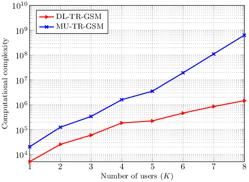
In Fig. 6, we present a computational complexity comparison of DL-TR-GSM and MU-TR-GSM for a varying number of users. We observe that DL-TR-GSM is capable of achieving a significant complexity reduction compared to MU-TR-GSM. The main reason for this is the ability of DL-TR-GSM to reduce the number of SVD computations and more notably the number of values (note that the number of different scaling coefficient values increases exponentially with for MU-TR-GSM). Hence, DL-TR-GSM has the potential to provide a very significant computational complexity reduction in real communication systems with a large number of users.
VII Conclusion
In this paper, we proposed a new multiuser MIMO scheme, referred to as DL-TR-GSM, based on the concept of DLT. In contrast to MU-TR-GSM which applies an activation of a subset of the receive antennas, DL-TR-GSM uses different power levels to transfer information in the receive spatial domain. This operational change provides a considerable complexity reduction in multiuser downlink communications. For the same reason, the hardware complexity of the user terminals decreases, causing a potentially large power saving. To further improve the performance of DL-TR-GSM, we proposed a separate detector which reduces the detection complexity, while maintaining a near-optimal BER.
References
- [1] R. Y. Mesleh, H. Haas, S. Sinanovic, C. W. Ahn, and S. Yun, “Spatial modulation,” IEEE Trans. Veh. Technol., vol. 57, no. 4, pp. 2228–2241, Jul. 2008.
- [2] M. Di Renzo, H. Haas, A. Ghrayeb, S. Sugiura, and L. Hanzo, “Spatial modulation for generalized MIMO: Challenges, opportunities, and implementation,” Proc. IEEE, vol. 102, no. 1, pp. 56–103, Jan. 2014.
- [3] A. Younis, N. Serafimovski, R. Mesleh, and H. Haas, “Generalised spatial modulation,” in Conf. Rec. of the 44th Asilomar Conf. on Signals, Syst. and Computers (ASILOMAR). IEEE, 2010, pp. 1498–1502.
- [4] L. L. Yang, “Transmitter preprocessing aided spatial modulation for multiple-input multiple-output systems,” in IEEE 73rd Veh. Technol. Conf. (VTC-Spring), May 2011, pp. 1–5.
- [5] N. S. Perović, P. Liu, and A. Springer, “Bit error probability of preprocessing aided spatial modulation based on MMSE precoding,” in IEEE 26th Int. Symp. on Personal, Indoor, and Mobile Radio Commun. (PIMRC), Hong Kong, Aug. 2015, pp. 819–823.
- [6] R. Zhang, L. L. Yang, and L. Hanzo, “Generalised pre-coding aided spatial modulation,” IEEE Trans. Wireless Commun., vol. 12, no. 11, pp. 5434–5443, Nov. 2013.
- [7] ——, “Error probability and capacity analysis of generalised pre-coding aided spatial modulation,” IEEE Trans. Wireless Commun., vol. 14, no. 1, pp. 364–375, Jan. 2015.
- [8] C. Masouros and L. Hanzo, “Dual-layered MIMO transmission for increased bandwidth efficiency,” IEEE Trans. Veh. Technol., vol. 65, no. 5, pp. 3139–3149, May 2016.
- [9] T. L. Narasimhan, P. Raviteja, and A. Chockalingam, “Generalized spatial modulation in large-scale multiuser MIMO systems,” IEEE Trans. Wireless Commun., vol. 14, no. 7, pp. 3764–3779, Jul. 2015.
- [10] S. Narayanan, M. J. Chaudhry, A. Stavridis, M. Di Renzo, F. Graziosi, and H. Haas, “Multi-user spatial modulation MIMO,” in 2014 IEEE Wir. Commun. and Net. Conf. (WCNC). IEEE, 2014, pp. 671–676.
- [11] K. M. Humadi, A. I. Sulyman, and A. Alsanie, “Spatial modulation concept for massive multiuser MIMO systems,” Int. Journal of Antennas and Propagation, vol. 2014, p. e563273, Jun. 2014.
- [12] A. Stavridis, M. D. Renzo, and H. Haas, “Performance analysis of multistream receive spatial modulation in the MIMO broadcast channel,” IEEE Trans. Wireless Commun., vol. 15, no. 3, pp. 1808–1820, Mar. 2016.
- [13] R. Pizzio, B. F. Uchôa-Filho, M. Di Renzo, and D. Le Ruyet, “Generalized spatial modulation for downlink multiuser MIMO systems with multicast,” in 2016 IEEE 27th Annual Int. Symp. on Personal, Indoor, and Mobile Radio Commun. (PIMRC). IEEE, 2016, pp. 1–6.
- [14] W. Liu, L.-L. Yang, and L. Hanzo, “SVD-assisted multiuser transmitter and multiuser detector design for MIMO systems,” IEEE Trans. Veh. Technol., vol. 58, no. 2, pp. 1016–1021, Feb. 2009.
- [15] C. Liu, L.-L. Yang, W. Wang, and F. Wang, “Joint transmitter–receiver spatial modulation,” IEEE Access, vol. 6, pp. 6411–6423, 2018.
- [16] G. H. Golub and C. F. Van Loan, Matrix computations. JHU Press, 2012.
- [17] N. S. Perović, W. Haselmayr, and A. Springer, “Low-complexity detection for generalized pre-coding aided spatial modulation,” in IEEE 82nd Veh. Technol. Conf. (VTC Fall). Boston: IEEE, 2015, pp. 1–5.
- [18] R. Méndez-Rial, C. Rusu, N. González-Prelcic, A. Alkhateeb, and R. W. Heath, “Hybrid MIMO architectures for millimeter wave communications: Phase shifters or switches?” IEEE Access, vol. 4, pp. 247–267, 2016.