A filamentary cascade model of the inertial range

We now summarize how we will set up and evolve the vorticity within such a program. We consider a single cascade initiated at time zero by a helical filament of circulation $\Gamma$. To have a finite kinetic energy we take the helical filament to be closed and wound on a torus as in figure 2(a). This is a bit of an artifice since we are interested in local interactions. We shall deal with the question of finite energy in section 4.

The equation for the points of the initial filament centreline in Cartesian coordinates is given by

$$\bm{R}(t)=((R+b\cos t)\cos(t/m),(R+b\cos t)\sin(t/m),b\sin t),\quad 0\leq t\leq 2\pi m.$$

(2)

This helix makes $m$ turns on the torus and $R=mc$ is the radius of the torus. We use $b$ and $c$ as the parameters of the helix and its length is approximately $2\pi m\sqrt{b^{2}+c^{2}}$, even though it is wrapped around a curve. The circular core of the filament, containing the vorticity, is taken to have core radius $r$, and a parameter $\epsilon=\tfrac{1}{2}r/\sqrt{b^{2}+c^{2}}$ will occur in our analysis of the cascade. We shall denote this initial helical structure by H and refer to it as the root filament of our cascade.

We describe the the splitting of filaments using a binary notation. H will split into two helices H[0] and H[1]; we call these the [0] helix and the [1] helix. The circulations of these two filaments will be $\Gamma[0]=\beta_{0}\Gamma$ and $\Gamma[1]=\beta_{1}\Gamma$ with $\beta_{0}+\beta_{1}=1$. Note that $\beta_{0}$ is the volume fraction of the the [0] helix relative to the root, since at the moment of splitting the two daughters have the length of the parent. Following the splitting, we assume that each daughter filament is stretched uniformly, by factors $s_{0}$ and $s_{1}$ respectively. These stretched filaments will also be closed filaments, with the [0] filament wrapped around the [1] filament. We emphasize that all vorticity is accounted for in the splitting. Our cascade preserves vorticity volume and hence does not produce a fractal (but does give what is sometimes referred to as a fat fractal). Three levels of splitting are depicted in figure 3.

It is at this stage that binary self-similarity is introduced. We specify that one turn of H[0] will be a copy of one turn of the root helix, but smaller by a factor $\lambda_{0}$ (in all dimensions, including the core size), and similarly for H[1] with factor $\lambda_{1}$. Since in general these scaling factors will not be the same, our model begins to differ significantly from the beta model and the general phenomenology of simple (non-statistical) K41 scaling.

Indeed, taking the stretching to be uniform, it is immediate from the scaling of the core radii that

$$\lambda_{0}=\sqrt{\beta_{0}/s_{0}},\quad\lambda_{1}=\sqrt{\beta_{1}/s_{1}}.$$

(3)

After stretching and establishment of the similitude, our structure will have $m[0]={ms_{0}/\lambda_{0}}$ turns of the [0] helix and $m[1]={ms_{1}/\lambda_{1}}$ turns of the [1] helix. (Although in general $m[0]$, $m[1]$ will not be integers, they will be large compared to one and the nearest integer will be taken as they play a minor role in the computations below.) The [0] helix now has length $2\pi m\sqrt{b^{2}+c^{2}}s_{0}$, since it has resulted from stretching the root helix by the factor $s_{0}$, and has parameters $b[0]$, $c[0]$. The [1] helix will have parameters $b[1]$, $c[1]$. As we have noted, the [0] helix may be regarded as wrapped around the the [1] helix.

We approximate this “helix” around a helix” as a “helix around a large circle of equal length.” Then we have, approximately

$$m[0]={2\pi m\sqrt{b^{2}+c^{2}}s_{1}\over 2\pi c[0]}={2\pi m\sqrt{b^{2}+c^{2}}s_{1}\over 2\pi\lambda_{0}c}={s_{0}\over\lambda_{0}}m.$$

(4)

Therefore $s_{0}>s_{1}$ and

$${b\over c}=\sqrt{\left(\frac{s_{0}}{s_{1}}\right)^{2}-1}.$$

(5)

Thus $b/c$, the inverse slope of the helices, is fixed from the stretching parameters throughout our structure, $2\pi b>2\pi c$ expressing the excess length needed to turn a line into a helix.

We shall also specify that that the pair of daughter helices, H[0], H[1] are together oriented along the path occupied by what we shall describe as the “ghost” of the root helix H — the root helix is no longer there, but the the daughter helices spiral about the region it previously occupied. This is important for the retention of the scales of variation of the vorticity and velocity fields as the cascade proceeds. In effect the pair of daughter helices should be regarded as merged into a restoration of the parent, when viewed on the scale of the parent. One way to achieve this is to take the [1] helix as wound on the ghost of the root helix. Then we would have $2\pi m[1]c[1]=2\pi m\sqrt{b^{2}+c^{2}}$ or $s_{1}=\sqrt{1+(b/c)^{2}}$. We have above also taken the [0] helix as wound around the [1] helix: the figure 3(b) depicts this configuration with the ghost of the parent from (a) shown, while in (c) only the two daughters are shown. Thus, combined with $(\ref{eq:boverc})$ we then obtain the geometrical constraint

$$s_{1}^{2}=s_{0}.$$

(6)

If, similarly $s_{0}^{2}=s_{1}$, then the H[1] may wrap around H[0]. We shall later see how well our cascade satisfies these constraints and use them to fix parameters of the model.

We are using the term “helix” rather loosely here, to describe a structure each of whose components consists in the small of helical turns. The only time we need to be specific about the geometry is in the calculation of the local transfer of energy, as discussed in the next section, as well as in the imposition of $(\ref{eq:geomconstr})$. We emphasize that in visualizing this cascade it must be kept in mind that our helices are filamentary, i.e. slender vortex tubes. The degree of slenderness is set by the root helix.

To assess the effect of binary splitting, consider how the velocity scales with eddy size. Since vorticity increases in each filament by the stretching factor, we have characteristic velocities $U[0]=\sqrt{s_{0}\beta_{0}}\;U$, $U[1]=\sqrt{s_{1}\beta_{1}}\;U$, where $U$ is the characteristic root velocity. Writing

$$U[0]/U=\sqrt{s_{0}\beta_{0}}=\lambda_{0}^{\alpha_{0}},\quad U[1]/U=\sqrt{s_{1}\beta_{1}}=\lambda_{1}^{\alpha_{1}},$$

(7)

we evaluate for $s_{0}=1.6,\;s_{1}=1.22,\;\beta_{0}=0.25$, numbers which will appear below, and obtain $\alpha_{0}=0.49$, $\alpha_{1}=0.145$. These values must be compared to the K41 scaling exponent of $1/3$. No single cascade step of the present model, for example from root to H[0] or root to H[1], will yield this scaling. But we shall see that the present model does give $\zeta_{1}=0.348$ for the above parameter values, close to K41. This emphasizes the importance of averaging over all elements of a cascade which combines two scaling factors. The point we highlight is that the resulting single scaling exponent is a statistical quantity, a fact which is widely recognized but not often emphasized when discussing phenomenology.

The cascade now continues by splitting of the two daughters H[0], H[1] into four granddaughter helices. The pair H[01], H[00] splits off from H[0], and H[10] and H[11] from H[1]. Here and below the digits read from left to right give the sequence of splittings, H[10] being wrapped around H[11]. The scale factors $\lambda_{0},s_{0}$ apply to derive H[10] from H[1], the scale factors $\lambda_{1},s_{1}$ similarly give H[11] from H[1]. We show in figure 4 these and subsequent steps in the binary cascade, mirroring the structures in physical space in figure 3.

We shall apply this formula first to the closed, filamentary, helical structures of our cascade. Consider first the filament with axis given by $(\ref{eq:helixgeom})$ and core radius $r$. The calculation of energy uses a classical regularization to deal with the singularity of the energy of vortex line. We give details in appendix A. The energy consists of two parts, external and internal. Since the filaments are slender, the external part is independent of the distribution of vorticity in the core. It can therefore be computed assuming that vorticity is concentrated at the core boundary. The result is

	$\displaystyle E_{\mathrm{ext}}\approx{\Gamma^{2}m\over 2}\bigg[\int_{\epsilon}^{\infty}\bigg($	$\displaystyle{b^{2}\cos\psi+c^{2}\over({4b^{2}\sin^{2}\tfrac{1}{2}\psi+c^{2}\psi^{2}})^{1/2}}-{{b^{2}}\cos\psi+c^{2}\over c\psi}\bigg)d\psi$
		$\displaystyle\qquad\qquad-{b^{2}\over c}\,{\rm Ci}(\epsilon)+{c\over 2}\int_{\epsilon/m}^{\pi}{\cos\psi\over\sin\tfrac{1}{2}\psi}\,d\psi\bigg],\quad m\gg 1.$		(9)

Here

$$\tfrac{1}{2}\int_{\epsilon/m}^{\pi}{\cos\psi\over\sin\tfrac{1}{2}\psi}\,d\psi=-\log\tan(\epsilon/4m)-2\cos(\epsilon/2m),$$

(10)

and

$$\mathrm{Ci}(z)=-\int_{z}^{\infty}\frac{\cos t}{t}\,dt$$

(11)

is the cosine integral.

For constant core vorticity the internal energy is

$$E_{\rm int}={m\Gamma^{2}\sqrt{b^{2}+c^{2}}\over 8}$$

(12)

to leading order.

We now consider the interaction energy between the two helices H[0] and H[1] that result from a splitting. This is obtained from $(\ref{eq:enercalc})$ when the $\bm{x}$ integration is over one filament and the $\bm{x}^{\prime}$ integration is over the other. Since the [0] helix is wound on a [1] helix, and the dimensions of the two, determined by the scaling factors, are of comparable order, we have a complicated intertwining of curves. We shall model it by replacing the H[1] by a ring of the same length, which then serves as the axis on which H[0] is wound. We denote the helix with subscript ‘$\mathrm{h}$’ and the ring with subscript ‘$\mathrm{r}$’. Thus we seek to compute

$$E_{\rm interact}={\Gamma_{\mathrm{h}}\Gamma_{\mathrm{r}}\over 4\pi}\int_{0}^{2\pi m}\!\!\!\int_{0}^{2\pi m}{\bm{t}_{\mathrm{h}}(t)\cdot\bm{t}_{\mathrm{r}}(t^{\prime})\over|\bm{R}_{\mathrm{h}}(t)-\bm{R}_{\mathrm{r}}(t^{\prime})|}\,dt\,dt^{\prime},$$

(13)

where

		$\displaystyle\bm{R}_{\mathrm{r}}(t)=(mc\cos(t/m),mc\sin(t/m),0),$		(14)
		$\displaystyle\bm{R}_{\mathrm{h}}(t)=((mc+b\cos t)\cos(t/m),(mc+b\cos t)\sin(t/m),b\sin t),$		(15)
		$\displaystyle\bm{t}_{\mathrm{h}}(t)\cdot\bm{t}_{\mathrm{r}}(t^{\prime})=-bc\sin t\sin[(t-t^{\prime})/m]+(c^{2}+(bc/m)\cos t)\cos[(t-t^{\prime})/m],$		(16)
		$\displaystyle|\bm{R}_{\mathrm{h}}(t)-\bm{R}_{\mathrm{r}}(t^{\prime})|=\big[b^{2}+(2mbc\cos t+2m^{2}c^{2})\big(1-\cos[(t-t^{\prime})/m]\big)\big]^{1/2},$		(17)

for $0\leq t\leq 2\pi m$. We will drop the term involving ${bc/m}$ in $(\ref{eq:tangs})$ and $2mbc$ in $(\ref{eq:Rs})$ as negligible at large $m$.

At this point the calculation proceeds similarly to the direct energy calculation, and is in fact simpler. We can divide into inner and outer contributions as follows:

	$\displaystyle E_{\rm interact}\approx{\Gamma_{\mathrm{h}}\Gamma_{\mathrm{r}}\over 2\pi}\int_{0}^{2\pi m}dt^{\prime}\bigg[$	$\displaystyle\int_{0}^{Am^{\alpha}}{c^{2}\over\sqrt{b^{2}+c^{2}(t-t^{\prime})^{2}}}\,d(t-t^{\prime})$
	$\displaystyle+$	$\displaystyle\int_{Am^{\alpha-1}}^{\pi}{-b\sin(t^{\prime}+m\psi)+c\cos\psi\over 2\sin\tfrac{1}{2}\psi}\,d\psi\bigg].$		(18)

We see that the $t^{\prime}$ term does not contribute under $t^{\prime}$ integration. Thus we obtain

$$E_{\rm interact}\approx\Gamma_{\mathrm{h}}\Gamma_{\mathrm{r}}mc\Big[\log{2cAm^{\alpha}\over b}-\log{Am^{\alpha-1}\over 4}-2\Big]=\Gamma_{\mathrm{h}}\Gamma_{\mathrm{r}}mc\Big[\log{8mc\over b}-2\Big].$$

(19)

We are now able to compute the energy (external plus internal plus interaction) of our system of H[0] and H[1]. Let the root energy, involving $m$ turns of the root helix, be $E$. Let H[0], involving $m[0]$ turns, have energy $E[0]$ in isolation, and similarly $E[1]$ for H[1]. Finally let $E[0,1]$ be the interaction energy of $m[0]$ turns of H[0] in the presence of a ring filament with the properties of H[1], and whose length is that of H[1]. Then the ratio of total energy of this system to the root energy is given by

$$E_{\rm total}/E=s_{0}\beta_{0}^{2}E[0]/E+s_{1}\beta_{1}^{2}E[1]/E+s_{0}\beta_{0}\beta_{1}E[0,1]/E.$$

(20)

Here the factors of $\beta_{0,1}$ are the scaling factors for circulation, obtained at the time of splitting, and before any stretching has occurred. The factors $s_{0,1}$ come from a product of the scaling by $\lambda_{0,1}$ in the size of one turn of the helix, and the scaling by $s_{0,1}/\lambda_{0,1}$ of the number of turns of the helix.

We shall make use of this formula in the section 4 to validate the approximate conservation of energy in the splitting of a helical filament. We note here that every term in the energy balance has the factor $\Gamma mc$ from the root filament. The remaining dependence upon $m$, and only dependence surviving in $(\ref{eq:totener})$, occurs in terms which contribute a logarithmic divergence. These logarithmic terms also contain the effect of filament slenderness through the parameter $\epsilon$. As a result the energy per unit turn of a filament and its daughters depends rather weakly on $m,\epsilon$.

This special case is of interest because of its simplicity. The geometry of the structures is the same whether they are generated by splitting into a [0] daughter or a [1] daughter; however the two branches are still not equivalent as we allow $\beta_{0}\neq\beta_{1}$ and so $s_{0}\neq s_{1}$: structures can be stretched by different amounts and so at each level $n$ of the hierarchy we have structures that have the same scale but different vorticity intensities and so different contributions to the structure function $Q_{p}(r)$. In the following we will often refer to scaling factors by the name of the quantity they scale, again effectively setting the root scales $U$, $L$ equal to unity. The structures of size $r=\lambda^{n}$ may now be identified with a given step $n$. These structures are space filling (have the total volume of the root filament), but appear at different times and have different lifetimes, of order $s_{0}^{-k}s_{1}^{-(n-k)}$, before breaking into smaller structures.

We shall compute $\zeta_{p}$ by imposing the four-fifths condition $\zeta_{3}=1$. The latter follows from the vanishing of a dissipation scaling parameter at $p=0$, which is a consequence of the assumption that the support of dissipation is finite in the limit of zero viscosity; see [5]. This condition also results from the independence of volume on the scale of the structures involved.

We now have the link $\lambda=\sqrt{\beta_{0}/s_{0}}=\sqrt{\beta_{1}/s_{1}}$ and we recall that velocity scales like $\lambda s_{0}$ or $\lambda s_{1}$ as we create [0] or [1] helices. We compute $(\delta u)^{p}$ by integrating $(\beta_{0}s_{0})^{pk/2}(\beta_{1}s_{1})^{p(n-k)/2}$ over the volume occupied by the structures of size $r=\lambda^{n}$, namely $\beta_{0}^{k}\beta_{1}^{n-k}$, multiplying by the number of such structures, and summing over $k$. Thus we have

	$\displaystyle Q_{p}(r)=\langle(\delta u)^{p}\rangle$	$\displaystyle=\sum_{k=0}^{n}{{n}\choose{k}}\beta_{0}^{k}\beta_{1}^{n-k}(\beta_{0}s_{0})^{pk/2}(\beta_{1}s_{1})^{p(n-k)/2}$		(24)
		$\displaystyle=\big[\lambda^{-p}(\beta_{0}^{p+1}+\beta_{1}^{p+1})\big]^{n}\sim r^{\zeta_{p}}=\lambda^{n\zeta_{p}}.$		(25)

The four-fifths law then implies

$$\lambda=\lambda^{-3}(\beta_{0}^{4}+\beta_{1}^{4}),$$

(26)

or $\lambda=(\beta_{0}^{4}+\beta_{1}^{4})^{1/4}$, with $s_{0,1}=\beta_{0,1}/\lambda^{2}$. Thus

$$\zeta_{p}={\log(\beta_{0}^{p+1}+\beta_{1}^{p+1})\over\log(\beta_{0}^{4}+\beta_{1}^{4})^{1/4}}-p.$$

(27)

We show in figure 6 this result for the optimal $\beta_{0}=0.438$ or 0.562. Taking $\beta_{0}=0.562$ we have $s_{0}=1.52,s_{1}=1.18$. The other values of $\beta$ shown in the figure illustrate what we shall find occurs more generally. For $\beta$ less than optimal, the $\zeta_{p}$ are too low. For larger values, the results lie close to K41. What is remarkable is how close we fall to the She–Leveque result at the optimal $\beta$. We note that once the constraint of equal $\lambda=\lambda_{0}=\lambda_{1}$ is relaxed, there will be a second free parameter (which we shall take to be $s_{0}$). Optimization is then over two parameters. An important condition of the cascade in stationary turbulence is that the flux of energy be constant. Here, we must sum for each daughter the volume fraction times velocity squared divided by a time, the latter being the inverse vorticity. Thus in terms of scaling factors the quantity

$$\bar{\varepsilon}=\beta_{0}^{2}s_{0}^{2}+\beta_{1}^{2}s_{1}^{2}$$

(28)

should be unity. Since here $s_{0,1}=\beta_{0,1}\lambda^{-2}$ we indeed find $(\beta_{0}^{4}+\beta_{1}^{4})\lambda^{-4}=1$. Note this constraint is equivalent here to the four-fifth’s law $(\ref{eq:45same})$ since $\lambda^{2}=\beta_{0,1}/s_{0,1}$

We also point out the connection made here to a single cascade. The case $\beta_{0}=0.5$ shown in figure 6 yields K41. But then, again since $s_{0,1}=\beta_{0,1}\lambda^{2}$, we have $s_{0}=s_{1}$. Thus all the daughter filaments are equivalent. This is the only example within our model of a single cascade. It yields K41 scaling for all $p$ with $\beta=1/2,s=\sqrt{2},\lambda=8^{-1/4}=0.5946$ The [0] helix cannot now wrap around the [1] helix. So a different structure is needed, for example taking both helices wrapped around the centerline of the parent but out of phase by half a turn.

We now consider the general case where $\lambda_{1}\neq\lambda_{0}$ and structures at each level $n$ of the cascade have varying scales. Bearing in mind the binomial weight and arguing as above, each set of branches labelled by $k$ and $n$ contributes an amount that scales as

$${{n}\choose{k}}\beta_{0}^{k}\beta_{1}^{n-k}(\beta_{0}s_{0})^{pk{/2}}(\beta_{1}s_{1})^{p(n-k){/2}}$$

(29)

to $Q_{p}(r)$ at the scale $r=\lambda_{0}^{k}\lambda_{1}^{n-k}$. We take the cascade to continue to an arbitrary number of levels $n\to\infty$, for this calculation relevant to the inviscid limit. Of course in reality the smallest filamentary scale is fixed at the Kolmogorov scale. We first give an approximate argument that gives numerical values for the scaling exponents $\zeta_{p}$ for $Q_{p}(r)\sim r^{\zeta_{p}}$. We will then refine the discussion below in section 4.3.

First, let us generalise to some general measurement $Q(r)$ and let $Q_{\lambda}$ be the scaling factor linked to an eddy of size scaling factor $\lambda$, so that the contribution in (29) above becomes

$${{n}\choose{k}}(\beta_{0}Q_{\lambda_{0}})^{k}(\beta_{1}Q_{\lambda_{1}})^{n-k}.$$

(30)

If we look at the contribution to $Q$ from all structures at level $n$ for all $k$, that is the contribution to $Q(r)$ integrated over all scales $r$, this is

	$\displaystyle(\beta_{0}Q_{\lambda_{0}}+\beta_{1}Q_{\lambda_{1}})^{n}$	$\displaystyle=\sum_{k=0}^{n}{{n}\choose{k}}(\beta_{0}Q_{\lambda_{0}})^{k}(\beta_{1}Q_{\lambda_{1}})^{n-k}$		(31)
		$\displaystyle=(\beta_{0}Q_{\lambda_{0}}+\beta_{1}Q_{\lambda_{1}})^{n}\sum_{k=0}^{n}{{n}\choose{k}}f_{0}^{k}f_{1}^{n-k},$		(32)

where

$$f_{0}=\beta_{0}Q_{\lambda_{0}}/(\beta_{0}Q_{\lambda_{0}}+\beta_{1}Q_{\lambda_{1}}),\quad f_{1}=\beta_{1}Q_{\lambda_{1}}/(\beta_{0}Q_{\lambda_{0}}+\beta_{1}Q_{\lambda_{1}}).$$

(33)

Now the inertial range analysis in terms of the exponents $\zeta_{p}$ is in the limit $r\rightarrow 0$. One might therefore simplify the calculation of the exponents by taking $n$ large and just considering the contributions from the single level $n$. The binomial distribution will then be sharply peaked and we can make use of the normal approximation to the binomial distribution,

$${{n}\choose{k}\,}f_{0}^{k}f_{1}^{n-k}\approx{1\over\sqrt{2\pi nf_{0}f_{1}}}\,e^{-{(k-nf_{0})^{2}/2nf_{0}f_{1}}}\,.$$

(34)

The peak contribution to $Q$ from structures at level $n$ comes from a scale $r=\lambda_{0}^{nf_{0}}\lambda_{1}^{nf_{1}}$. The approximation then consists of equating the total contribution (31) to $Q$, to the value of $Q(r)$ at this dominant scale $r$; in other words we set

$$Q(r)=(\beta_{0}Q_{\lambda_{0}}+\beta_{1}Q_{\lambda_{1}})^{n},\quad r=\lambda_{0}^{nf_{0}}\lambda_{1}^{nf_{1}}.$$

(35)

The scaling exponent $\zeta_{Q}$ linked to $Q(r)$ is then defined by

$$\beta_{0}Q_{\lambda_{0}}+\beta_{1}Q_{\lambda_{1}}=\Upsilon^{\zeta_{Q}},\quad\Upsilon=\lambda_{0}^{f_{0}}\lambda_{1}^{f_{1}},$$

(36)

where $f_{0},f_{1}$ are determined by the quantity being averaged through $(\ref{eq:fg})$, giving explicitly

$$\zeta_{Q}=\frac{(\beta_{0}Q_{\lambda_{0}}+\beta_{1}Q_{\lambda_{1}})\log(\beta_{0}Q_{\lambda_{0}}+\beta_{1}Q_{\lambda_{1}})}{\beta_{0}Q_{\lambda_{0}}\log\lambda_{0}+\beta_{1}Q_{\lambda_{1}}\log\lambda_{1}}\,.$$

(37)

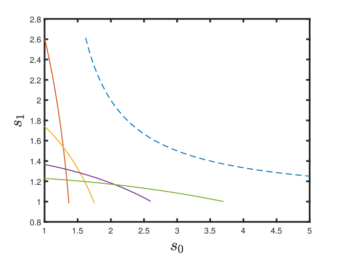
For velocity structure functions, $Q_{\lambda_{0}}=(\beta_{0}s_{0})^{p/2}$, $Q_{\lambda_{1}}=(\beta_{1}s_{1})^{p/2}$, for $p=1,2,3\dots.$, with now $\zeta_{Q}=\zeta_{p}$. In particular the four-fifths law may now be stated as

$$\beta_{0}^{5/2}s_{0}^{3/2}+\beta_{1}^{5/2}{s_{1}}^{3/2}=\Upsilon=\lambda_{0}^{\beta_{0}^{5/2}s_{0}^{3/2}\over\beta_{0}^{5/2}s_{0}^{3/2}+\beta_{1}^{(5/2)}{s_{1}}^{3/2}}{\lambda_{1}}^{\beta_{1}^{5/2}{s_{1}}^{3/2}\over\beta_{0}^{5/2}s_{0}^{3/2}+\beta_{1}^{5/2}{s_{1}}^{3/2}}.$$

(38)

Recall that $\lambda_{0}=\sqrt{\beta_{0}/s_{0}}$ and $\lambda_{1}=\sqrt{\beta_{1}/s_{1}}$. Thus $(\ref{eq:45law})$ is a relation between $\beta_{0}$, $s_{0}$, $s_{1}$. In figure 7 we show this relation. In general to compute structure coefficients we choose $\beta_{0}$, $s_{0}$, $\beta_{1}=1-\beta_{0}$, find the $s_{1}$ which enforces the four-fifths law, and then for fixed $\beta_{0}$ vary $s_{0}$ until we get good agreement with the She–Leveque formula in a suitable norm; here and below we use the $l^{2}$ norm, that is the root mean square, but very close results are obtained with the $l^{1}$ norm. We thus obtain a one-parameter family of “optimal” cascades with parameter $\beta_{0}$. We have the condition that $s_{0}>s_{1}$ but we also see from figure 7 that the inequality $s_{0}+s_{1}>s_{0}s_{1}$ is easily satisfied for the values we use. We shall make use of this inequality in section 5.

The above calculation of scaling exponents, yielding (37), is approximate as the peak contribution to $Q_{p}(r)$ is not quite at the value of $n$ determined above; however values obtained for key quantities are correct to a few percent. We give a more detailed calculation, which includes the correction to the peak contribution below, in section 4.3. For simplicity, in the tables and figures that follows we use results only from the later, improved calculation.

We next wish to investigate families of models that satisfy the four-fifths law and give structure exponents close to those of She–Leveque in (1). We obtain a 1-parameter family of models parameterised by $\beta_{0}$. To do this systematically we first fix $\beta_{0}$ and so $\beta_{1}=1-\beta_{0}$. We then vary $s_{0}$ and calculate $s_{1}$ via imposing the four-fifths law $\zeta_{3}=$ (done in (54) below). We then have a model defined by $(\beta_{0},\beta_{1},s_{0},s_{1})$: we proceed to calculate the structure exponents $\zeta_{p}$ for $p=1,2,\ldots 10$ (via (53)) and measure the $l^{2}$ error for these compared with the She–Leveque ones in (1). For a given $\beta_{0}$ that error is now a function of $s_{0}$, and we vary $s_{0}$ to minimise the error. Once we have done this we obtain a branch of solutions parameterised by $\beta_{0}$.

Our results are shown in table 1 and figure 8, and surprisingly we find two solution branches of acceptable cascade models. Figure 8(a) shows values of $s_{0}$ as solid blue/red curves for the lower/upper branches, as functions of $\beta_{0}$. The dashed curves show the corresponding values of $s_{1}$: note that the solution branches are related by the reflection symmetry in the line $\beta_{0}=\tfrac{1}{2}$, that is $\beta_{0}\leftrightarrow\beta_{1}$, $s_{0}\leftrightarrow s_{1}$. The fit to the She–Leveque scalings exponents is excellent for both branches, with the $l^{2}$ (rms) error depicted in figure 8(b). The remarkable agreement suggests that our models realise physically the assumptions underlying the She–Leveque result.

Further analysis of the two branches is given in 1. For the lower branch (the values below the middle horizontal line, blue curve in figure 8), we rejected larger values of $s_{0}$ as giving an extremely tight [0] helix ($m[0]/m\approx 16$ when $s_{0}=3$). For the upper branch (values above the line, red curve in figure 8), we did not find solutions below $\beta_{0}\approx 0.33$. Note the last two column, for $s_{0}/s_{1}^{2}$ and $s_{1}/s_{0}^{2}$, eliminate the upper branch if the one helix is to wrap around the other. On the lower branch, these constraint allow two values a $\beta_{0}$, one slightly smaller than $0.25$, the other at $0.41$, with alternate wrapping of the two daughter helices. These values then determine the bimodal cascades of choice in this model.

While this calculation in the previous section leading to the formula (37) for $\zeta_{p}$ is useful for exploring the parameter space of cascades, it makes a small error of a few percent in the $s_{(}0,1)$, though increasing for the smaller $\beta_{0}$ values on the lower branch. The reason for the error lies in the contributions from multiple levels of the cascade to the eddy size $r$. It might be thought that these would be negligible at large $n$. However the sharp peak in the binomial distribution forces contributions below the largest $n$ to lie in the tails of the distribution. This requires an application of large deviation theory and use of Stirling’s formula in the binomial coefficients.

We now describe this precise calculation of scaling exponents for large $n$ over a range of cascade levels. If we fix a scale $r\ll 1$ then contributions to $Q(r)$ will come from a range of levels $n$, those for which $\lambda_{0}^{n}\leq r\leq\lambda_{1}^{n}$ or $n_{-}\leq n\leq n_{+}$, taking $\lambda_{0}<\lambda_{1}$ without loss of generality. For each level $n$ where there is a contribution, this will arise from structures labelled by $k$ with $r\simeq\lambda_{0}^{k}\lambda_{1}^{n-k}$ (or nearby values of $k$), as depicted in figure 5. Thus, as far as we need for a scaling argument we can write

$$Q(r)=\sum_{n=n_{-}}^{n_{+}}\begin{pmatrix}n\\ k\end{pmatrix}(\beta_{0}Q_{\lambda_{0}})^{k}(\beta_{1}Q_{\lambda_{1}})^{n-k}\bigg|_{k=k(r,n)}$$

(39)

with

$$k(r,n)=\mathrm{round}\left[\frac{\log r-n\log\lambda_{1}}{\log(\lambda_{0}/\lambda_{1})}\right];$$

(40)

as we vary $n$ we are also varying $k$ to maintain a fixed scale. Setting $b_{0}=\beta_{0}Q_{\lambda_{0}}$, $b_{1}=\beta_{1}Q_{\lambda_{1}}$ for brevity, we first use Stirling’s formula to write

		$\displaystyle\begin{pmatrix}n\\ k\end{pmatrix}b_{0}^{k}b_{1}^{n-k}=\frac{1}{(2\pi n)^{1/2}(k/n)^{1/2}(1-k/n)^{1/2}}\exp F(n),$		(41)
		$\displaystyle F(n)=n\log n-k\log k-(n-k)\log(n-k)+k\log b_{0}+(n-k)\log b_{1}.$		(42)

We are now able to replace $k$ and $n$ by continuous variables linked by

$$k(r,n)=\alpha_{0}n+\gamma,\quad n-k=\alpha_{1}n-\gamma,$$

(43)

where

$$\alpha_{0}=-\frac{\log\lambda_{1}}{\log(\lambda_{0}/\lambda_{1})}\,,\quad\alpha_{1}=\frac{\log\lambda_{0}}{\log(\lambda_{0}/\lambda_{1})}\,,\quad\gamma=\frac{\log r}{\log(\lambda_{0}/\lambda_{1})}\,,$$

(44)

noting that $\alpha_{0}+\alpha_{1}=1$. With $k$ linked to $n$ via (43), we then have that

$$Q(r)=\int_{-\infty}^{\infty}\frac{\exp F(n)}{(2\pi n)^{1/2}(k/n)^{1/2}(1-k/n)^{1/2}}\,dn,\quad k=k(r,n).$$

(45)

The contribution is peaked around the maximum of $F(n)$ at say $n=\bar{n}$, in other words where

$\displaystyle F^{\prime}(\bar{n})$

$\displaystyle=\log\bar{n}-\alpha_{0}\log(\alpha_{0}\bar{n}+\gamma)-\alpha_{1}\log(\alpha_{1}\bar{n}-\gamma)+\alpha_{0}\log b_{0}+\alpha_{1}\log b_{1}=0,$

(46)

and we have

$\displaystyle F(\bar{n})$

$\displaystyle=[\log(\lambda_{0}/\lambda_{1})]^{-1}\bigl[-\log[(\alpha_{0}+\gamma/\bar{n})/b_{0}]+\log[(\alpha_{1}-\gamma/\bar{n})/b_{1}]\bigr]\log r.$

(47)

In a scaling argument we can ignore algebraic prefactors and focus on the exponential dependence on $F$, to yield

$$Q(r)\sim\exp F(\bar{n})\sim r^{\zeta_{Q}}.$$

(48)

To tidy this up, set

$$\bar{n}/\log r=\delta^{-1},\quad\ell=\log(\lambda_{0}/\lambda_{1}),$$

(49)

and then in a calculation of a scaling exponent we first obtain $\bar{n}$ or equivalently $\delta$, which means solving

$\displaystyle-\log\lambda_{1}\log[(\delta-\log\lambda_{1})/b_{0}\ell]+\log\lambda_{0}\log[(\log\lambda_{0}-\delta)/b_{1}\ell]=0$

(50)

for $\delta$, and then substituting to obtain

$\displaystyle\zeta_{Q}=\ell^{-1}\bigl[-\log[(\delta-\log\lambda_{1})/b_{0}\ell]+\log[(\log\lambda_{0}-\delta)/b_{1}\ell]\bigr].$

(51)

These two equations are linear in the terms involving the logarithm of $\delta$ and other quantities; these may be solved and then $\delta$ eliminated to leave

$$b_{0}\lambda_{0}^{-\zeta_{Q}}+b_{1}\lambda_{1}^{-\zeta_{Q}}=1.$$

(52)

For any choices of $\lambda_{(}0,1)$ and $b_{(}0,1)=\beta_{(}0,1)Q_{\lambda_{(}0,1)}$ giving the quantity $Q$ we wish to measure, this is the implicit equation for $\zeta_{Q}$.

For the case of the $Q_{p}$ and exponents $\zeta_{p}$ we have $b_{0,1}=\beta_{0,1}^{p/2+1}s_{0,1}^{p/2}$, $\lambda_{0,1}=(\beta_{0,1}/s_{0,1})^{1/2}$ and so this becomes

$$\beta_{0}^{(p-\zeta_{p})/2+1}s_{0}^{(p+\zeta_{p})/2}+\beta_{1}^{(p-\zeta_{p})/2+1}s_{1}^{(p+\zeta_{p})/2}=1.$$

(53)

Imposing $\zeta_{3}=1$ gives a particularly straightforward equation, namely

$$\beta_{0}^{2}s_{0}^{2}+\beta_{1}^{2}s_{1}^{2}=1.$$

(54)

giving $s_{1}$ explicitly in terms of $s_{0}$ and $\beta_{0}$ and making $\bar{\varepsilon}_{\mathrm{total}}=1$. We thus have established exact constancy of energy flux when $Q_{p}(r)$ is determined precisely. We note that, when $\lambda_{0}=\lambda_{1}=\lambda$, (53, 54) yield our previous results for this special case. This is not surprising since (53, 54) are precise for large $n$ and the special case applies to any $n$.

References

- [1] Frisch, U. Turbulence, Cambridge, 1995.
- [2] Eyink, G.L. Local 4/5 law and energy dissipation anomaly in turbulence. Nonlinearity 15, 137–145, 2003.
- [3] Duchon, J. and Robert, R. Inertial energy dissipation for weak solutions of incompressible Euler and Navier-Stokes equations. Nonlinearity 13, 249–255, 2000.
- [4] Childress, S. A vortex-tube model of eddies in the inertial range. Geophys. Astrophys. Fluid Dynam. 29, 29–64, 1984.
- [5] She, Zhen-Su and Leveque, Emmanuel. Universal scaling laws for fully developed turbulence. Phys. Rev. Lett. 72, 336–339, 1994.
- [6] Lungren, T.S. Strained spiral vortex model for turbulent fine structure. Phys. Fluids 25, 2193–22013, 1982.
- [7] McKeown, R., Ostilla-Mónico, R., Pumir, A., Brenner, M.P. and Rubinstein, S.M. Cascade leading to the emergence of small structures in vortex ring collisions. Phys. Rev. Fluids 3, 124702, 2008.
- [8] McKeown. R.,Ostilla-Mónico, R., Pumir, A., Brenner, M.P., and Rubenstein, S.M. Turbulence generation through an iterative cascade of the elliptical instability. ArXiV preprint.
- [9] Sreenivasan, K. R., Vainshtein, S. I., Bhiladvala, R.,San Gil, Chen, S. and Cao, N. Asymmetry of velocity increments in fully developed turbulence and the scaling of low-order moments. Phys. Rev. Lett. 77, 1488–1491, 1966.
- [10] Saffman, P.G. Note on the decay of homogeneous turbulence. Phys. Fluids 10, 1349, 1967.
- [11] Moffatt, H.K. The degree of knotedness of tangled vortex lines. J. Fluid Mech. 35, 117–129, 1969.
- [12] Dubrulle, B. Intermittency in fully developed turbulence: Log-Poisson statistics and generalized scale invariance. Phys. Rev. Let. 73, 959–962, 1994.