Soft leptogenesis in the NMSSM with a singlet right-handed neutrino superfield
Abstract
In this work, we explore soft leptogenesis in the NMSSM framework extended by a right-handed neutrino superfield. We calculate the CP asymmetry, , and find it to be non-zero at tree-level without using thermal effects for the final state particles. This is in contrast to soft leptogenesis in the MSSM extended by a right-handed neutrino superfield where thermal effects are essential. The difference arises due to the presence of a 3-body decay of the sneutrino in the NMSSM that violates lepton number at tree-level. Apart from this, we also find that if the additional singlet scalar has a complex vacuum expectation value while all the other NMSSM parameters including the soft SUSY breaking ones relevant for CP asymmetry remain real. We estimate the order of magnitudes of these parameters to produce sufficient baryon asymmetry of the Universe.
I Introduction
It is well known that the observable Universe has an asymmetry between baryons and anti-baryons Tanabashi et al. 2018, often called the problem of baryogenesis. Over the years, many mechanisms have been proposed to create this baryon asymmetry. More recently, leptogenesis Fukugita and Yanagida 1986; Strumia 2006 has become a highly favoured model for baryogenesis, specially because this mechanism is naturally linked to neutrino masses. Adding right-handed (RH) singlet heavy neutrinos to the standard model (SM) generates neutrino masses by the seesaw mechanism Minkowski 1977; Mohapatra and Senjanovic 1980; Yanagida 1979; Gell-Mann et al. 1979; Glashow 1980; Schechter and Valle 1980. These RH neutrinos can also decay to produce a scalar and SM leptons and if the decay violates CP for example due to interference between tree-level and loop-level decays owing to complex couplings, a lepton asymmetry is generated. Since, in the SM, the symmetry is exact while the symmetry is broken by the electroweak (EW) sphaleron processes (Kuzmin et al. 1985), these sphaleron processes can convert the generated lepton asymmetry to baryon asymmetry.
Soft leptogenesis Grossman et al. 2003; D’Ambrosio et al. 2003; Fong et al. 2011a pertains to generating lepton asymmetry at the tree-level itself due to mixing between the particle and anti-particle states of the RH singlet sneutrino, , because of the presence of soft SUSY breaking terms11 1 Soft leptogenesis in different types of SUSY framework can be found in Chen and Mahanthappa 2004; Chun and Scopel 2006; Medina and Wagner 2006; Garayoa et al. 2007; Fong and Gonzalez-Garcia 2008; Fong and Gonzalez-Garcia 2009; Kajiyama et al. 2009; Fong et al. 2010; Hamaguchi and Yokozaki 2011; Fong et al. 2011b; Kuismanen and Vilja 2013.. In the most minimal soft leptogenesis setup using minimal supersymmetric standard model (MSSM) Chung et al. 2005; Martin extended by one RH neutrino superfield, , a CP asymmetry in the RH sneutrino sector is created only when thermal masses for the final products are considered. The asymmetry is present because the thermal phase space factors are different for bosons and fermions. Another work featuring soft leptogenesis looks at CP violation not just due to mixing between particle and anti-particle initial states but in decays and in the interference of mixing and decay Grossman et al. 2004. In Ref. Adhikari et al. 2015, it is shown that considering most generic soft trilinear couplings and one loop self energy contributions for sneutrino decay it is possible to generate CP violation even without finite temperature effects within the same setup.
However, the MSSM suffers from the so-called -problem Kim and Nilles 1984 – there is no explanation to why the SUSY scale preserving -term (a direct SUSY mass term for the Higgs fields) should be of the same order as the soft SUSY breaking terms. The most straightforward solution to the -problem comes by promoting the -parameter into a field whose vacuum expectation value (vev) is determined, like the other scalar field vevs, from the minimization of the scalar potential along the new field direction Ellwanger et al. 2010. Naturally, it is expected to fall in the range of the other vevs, i.e., of order . The next-to-minimal supersymmetric standard model (NMSSM) (for review see Ellwanger et al. 2010; Maniatis 2010) is the most simple and elegant model to solve this problem, where a singlet superfield is introduced to the MSSM superfields which gets non-zero vev. The NMSSM can be extended by a set of RH neutrino superfields to generate masses for the SM light neutrinos by the type-I seesaw (see Grossman and Haber 1997; King 1998; Kitano and Oda 2000 for the MSSM extended by RH neutrino superfield). This has been explored earlier in Ref. Das and Roy 2010. This extension also keeps the R-parity conserved if the sneutrinos do not get vevs Das and Roy 2010.
In this work, by using the NMSSM extended by the RH neutrino superfield, we present a soft leptogenesis scenario that creates a lepton asymmetry at the tree-level decay of the RH sneutrino without using thermal mass factors. The CP violation is achieved by the mixing between the particle and anti-particle states. This is due to the presence of the soft terms and the trilinear coupling between the additional singlet superfield which takes a vev and the RH neutrino superfield. A similar non-SUSY setup with such a trilinear term can be found in Alanne et al. 2019. We also show that it is possible to obtain non-zero CP asymmetry even when all the soft parameters are real. Since the soft terms are responsible for creating the CP asymmetry instead of needing flavour effects as in usual leptogenesis, using only one generation of the RH neutrino superfield is enough. Even so, the setup can be easily extended to get the experimentally observed SM neutrino mass hierarchies and their mixing angles pattern Esteban et al. 2017; de Salas et al. 2018.
The paper is organised in the following manner. We setup the model and segregate the parts required for soft leptogenesis in the next section (Sec. II). In the one following that, i.e., Sec. III, we calculate the CP asymmetry produced by decays of the various particle present in the model that contribute to non-zero CP asymmetry parameter at the tree-level. We talk about the decays of as well as the scalar in the model. In Sec. IV, we discuss the most crucial and important constraints and give a simple expression for . In Sec. V, we give and discuss the results of our calculation. We find that for successfully generating the observed baryon asymmetry of the Universe, we need . We also discuss what this could mean for various parameters of the model including the soft ones. We finally conclude in Sec. VI.
II Model
In the NMSSM, an extra singlet superfield is added to the MSSM Higgs sector Ellwanger et al. 2010. Assuming explicitly symmetry, the superpotential for the NMSSM with a singlet RH neutrino superfield in terms of the new singlet superfield and the MSSM doublet superfields and will be as follows Ellwanger et al. 2010:
| (1) |
where and are the doublet superfields of leptons and quarks; and denote singlet down (up)-type quark superfields, respectively, and ’s, ’s and are dimensionless couplings with generation indices (). After the singlet obtains a vacuum expectation value (vev) , an effective -term is generated: , which solves the so-called -problem Kim and Nilles 1984. The soft SUSY-breaking Lagrangian is given by
| (2) |
where and are the scalar components of and superfields, respectively. CP is spontaneously violated when the scalars attain vevs with relative physical phases. The vev of the singlet is complex:
| (3) |
Since leptogenesis occurs above the electroweak (EW) phase transition, we do not give vevs to the two Higgs doublets. In this case, spontaneous CP violation can occur only when .
II.1 Terms relevant for soft leptogenesis
The terms from the superpotential required for leptogenesis via sneutrino decay are:
| (4) |
Here we consider to be all real and positive. We also remove the indices from the leptons and the index from the Higgs superfield for brevity. The scalar potential is obtained using:
| (5) |
with
| (6) | ||||
| (7) | ||||
| (8) |
The fermionic part of the Lagrangian is given by:
| (9) |
The soft SUSY-breaking Lagrangian terms that play a role in leptogenesis are:
| (10) |
The superpotential and the soft breaking terms combine to give the following interactions for and which could in principle contribute to soft leptogenesis due to mixing between the particle and anti-particle states through the soft terms:
| (11) |
where .
III CP asymmetry
Because of the soft terms as well as the vev of , there is a mixing between particle and anti-particle states of the sneutrino and the singlet scalar which is the dynamic part of . The squared mass matrices for the two of them are given by:
| (12) | |||||
| (13) |
where
| (14) |
If is real, the mass square eigenvalues of the sneutrino are:
| (15) |
which have the following eigenstates:
| (16) |
Similarly, one can write the mass square eigenvalues and eigenstates for the system. Because of mixing between the particle and anti-particle states of sneutrino and singlet scalar, these systems are similar to and systems Nir 2001. The evolution of these systems in the non-relativistic limit are driven by the Hamiltonian defined as follows:
| (17) |
where is the mass matrix and is the decay rate matrix of the corresponding system.
Finally, the decay rates of the time evolved particle and anti-particle states of the and the system are calculated to get the final total CP asymmetry. As can be seen from Eq. (II.1), both and can decay to produce lepton asymmetry depending on the nature of their couplings. Therefore, we separately consider the two limiting cases where only one of them can decay at a time by fixing their masses. The first case is when . In this case, decays to produce the CP asymmetry at the tree-level while decays of into a pair of RH (s)neutrinos are kinematically suppressed. The relevant Feynman diagrams for this situation are shown in Figs. 1 and 2. Fig. 1 shows the point interaction, 2 and 3 body decays of while Fig. 2 shows the other possible 3-body decays of that are mediated by an off-shell . The first three point interactions of Fig. 1 are present in MSSM soft-leptogenesis as well and the observed matter-anti-matter asymmetry requires the decay products to have thermal corrections. The last diagram of Fig. 1 and those in Fig. 2 are presnt only in NMSSM. We will see in Sec. III.1 that the 3-body decay diagram of Fig. 1 is responsible for creating enough CP asymmetry without any thermal mass corrections. The contribution of diagrams in Fig. 2 is suppressed by the higher order soft terms. The second possibility to create the CP asymmetry is through decays of which occurs when . The diagrams are shown in Fig. 3. However, as we will see in Sec. III.2, these decays can not produce any CP asymmetry at the tree-level via the same mechanism followed by decays. This tells us that we can ignore the decays of without any loss of generality for the study of soft leptogenesis in the present setup. We consider these cases one-by-one.
III.1 decays
Irrespective of the mass of relative to the mass of , the sneutrino can decay into leptonic (sleptonic) and Higgs (Higgsino) final particles. The CP asymmetry generated from such a scenario was calculated in Grossman et al. 2003; D’Ambrosio et al. 2003. However, if , the 3-body decay channel shown in the last Feynman diagram of Fig. 1 opens up and it leads to interesting consequences for soft leptogenesis as we show below.
For the snuetrino system, upto leading order in the off-diagonal terms22 2 Considering and much smaller compared to and respectively as will be justified later., the mass matrix can be calculated from the squared mass matrix in Eq. (12):
| (18) |
The decay rate matrix can be written from the Eq. (II.1). It contains both diagonal as well as off-diagonal terms because can decay into particle as well as anti-particle final states.
| (19) |
with,
| (20) |
The parameter and in matrix are associated with the 3-body decay contributions of given by,
| (21) | ||||
| (22) |
The logarithm in can be expanded for the soft term at least an order of magnitude smaller than (this can be assumed without any loss of generality as later to draw our conclusions and compare with MSSM soft-leptogenesis in D’Ambrosio et al. 2003; Fong et al. 2011a; Grossman et al. 2003, we will be restricting to leading order in soft-terms) to give:
| (23) |
Under the same approximation used for and with , becomes:
| (24) |
It is important to note that as long as the soft term is sufficiently small compared to (at least by an order of magnitude) or the phase , .
There are 4 terms in of Eq.(21) which represents the contribution of decay, where the first two terms come from the 3-body decay arising from the point interaction in Fig. 1 while the third term comes from the second diagram of Fig. 2. The last term in comes from the interference of these two diagrams. The in Eq.(22) appears in the decay matrix due to the presence of first and the third diagrams of Fig. 2. It is pertinent to note here that is at least quadratic in the soft terms and . One could in principle have higher order diagrams relating to 4 or more decay products. However, all such diagrams will be suppressed heavily by higher powers of .
The solutions for the time evolution of and come from the Schrodinger like equation
| (25) |
where . The solutions are obtained as,
| (26) | |||||
| (27) |
where are the field values at and
| (28) | |||||
| (29) | |||||
| (30) |
Let’s define and and . Then if which happens when (typically of to satisfy neutrino mass bounds), we can write
| (31) | |||||
| (32) |
If as well, the argument of the trigonometric functions becomes such that we can write:
| (33) | |||||
| (34) |
where
| (35) | |||||
| (36) |
The Eqs. (33) and (34) are substituted back in Eq. (II.1) for calculating the CP asymmetry factor which is defined as the ratio of the difference between the decay rates of and into final state particles with lepton number and to the sum of all the decay rates, i.e.,
| (37) |
where are the final states with lepton number and , respectively. This then gives us the following CP asymmetry parameter:
| (38) |
The decay rates at the tree-level itself for final states with lepton numbers are different because the factor as it is not a hermitian quantity. This requires non-zero off-diagonal terms to be present in the mass matrix as well as the decay rate matrix of the system with atleast one of them being complex.
The sum and difference of the ratios and can be written as:
| (39) | |||||
| (40) |
where
| (41) | |||||
| (42) |
Keeping terms upto the leading order in , we find that the sum of the ratios is while the difference is twice the values of with,
| (43) |
such that the final CP asymmetry can be written as:
| (44) |
where is defined as . From Eqs. (43) and (44) it is evident that there is a non-zero CP asymmetry even with real , provided is sufficiently large.
We also note that while the usual soft leptogenesis done in the MSSM Grossman et al. 2003; D’Ambrosio et al. 2003, to the leading order in soft terms (), necessarily requires thermal phase space factors for the final state bosons () and fermions () to have , we get an asymmetry even without thermal mass corrections to the decay products at the leading order in soft terms. This happens because of the presence of in the model which facilitates a 3-body decay of which is not cancelled by the other terms. If we did not have this, at leading order in soft terms, and there would be no asymmetry without thermal mass corrections. At the leading order in the soft terms ( is negligible), is
| (45) |
It is clear from Eq. (45) that the only contribution coming from diagrams of Fig. 2 are coming from the cross term of the second diagram with the last diagram of Fig. 1 through . Even in , the dominant contribution comes through the 3-body decay by the vertex interaction of Fig. 1. Therefore it is possible to successfully generate non-zero lepton asymmetry from system at the tree-level without using thermal phase space factors for bosonic and fermionic final states. We discuss this more and give some numerical estimates in Sec. V for relevant parameters. For the moment, let’s consider the decays of .
III.2 decays
Unlike the decays where most of the decay products were massless, the final products of decay are massive, as shown in Fig. 3. This creates two possible decay modes of according to the condition satisfied.
- 1.
decays to and . This happens when ,
- 2.
decays only to . This happens when .
The mass matrix and the matrix of the system are respectively:
| (46) |
where
| (47) | ||||
A non-relativistic Hamiltonian can be defined following Eq. (17). Immediately it can be seen that because of the absence of an off-diagonal term in the decay rate matrix of , the ratio corresponding to of decay,
| (51) |
If we solve for the evolution of the system, the CP asymmetry parameter computed exactly analogously to the system will be zero because of exact cancellation between the ratios and . Thus
| (52) |
IV General Constraints
The CP asymmetry in this model depends on a lot of parameters. However, we can constrain some of them by various considerations. In deriving the following general constraints, we take , and for reasons that will become clear later in Sec. V.
- •
- •
The way we derived the CP asymmetry requires well separated states D’Ambrosio et al. 2003, i.e., as well as as stated before. This gives us two self-consistent limits:
(56) (57) - •
Neutrino mass upper limits ( eV Aghanim et al. 2018; Tanabashi et al. 2018) put constraints on the Yukawa coupling strength and the mass of the RH (s)neutrino.
(58) - •
Electric dipole moment (EDM) calculations can constrain the CP violating phases that appear in the vevs of the two Higgs doublets and the scalar singlet . In Ref. Huitu et al. 2012, they show that in principle (the phase in the vev of should we go below the EW scale) and could be large as long as the relative phase is kept small. For more details about the EDM constraints on the NMSSM, see King et al. 2015.
IV.1 A simpler form for
We can write a simpler form for the CP asymmetry by using the approximations made and the general relationships between various parameters given above. The set of parameters governing are:
| (59) |
We choose the soft masses TeV and to be of GeV with . This along with means both . Therefore, from Eq. (58), one can put an upper limit on , i.e., . With these choices and approximations the form of can be simplified to
| (60) |
V Results and discussions
To obtain the baryon asymmetry of the Universe, , we solve the simultaneous Boltzmann equations for the number density, , and the number density, , which are as follows Buchmuller et al. 2005; Garayoa et al. 2009; Hahn-Woernle et al. 2009:
| (61) | |||||
| (62) |
where is the Hubble parameter at with and is the equilibrium number density of . They take the following forms:
| (63) | |||||
| (64) |
with GeV being the Planck mass and is the number of relativistic degrees of freedom in the NMSSM which we take except for the which is non-relativistic. In writing the Boltzmann equation for number density, we neglect the scattering processes for washout and assume it is dominated mostly by inverse decays. The contribution to washout from the scattering processes is small because we are in the weak washout regime with . The final number density thus created, then converts to the baryon asymmetry by the sphaleron processes such that the ratio of the baryon number density to the photon number density, , is:
| (65) |
where , is the effective number of relativistic degrees of freedom at recombination and is the sphaleron conversion factor. Since we will solve the Boltzmann equations numerically, we use the complete form of given in Eq. (44).
In Fig. 4, we show the typical value of the CP asymmetry that satisfies the observed baryon asymmetry of the Universe. It turns out that we need to get the correct observed baryon asymmetry while satisfying neutrino mass bounds. This value of is similar to the one obtained by other vanilla leptogenesis scenarios in the weak washout regime. The only difference is that usual leptogenesis occurs with decays at the loop-level interfering with tree-level decays due to complex Yukawa couplings that violate CP. In the soft leptogenesis, the Yukawa parameter could very well remain real as the source of CP asymmetry lies elsewhere – in the time-varying mixing between and states due to the complex nature of and the soft SUSY breaking parameters.
V.1 Case 1: is near zero
To get we fix the values of the following parameters in line with the earlier approximations and constraints:
| (66) |
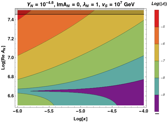
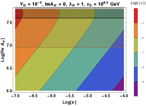
For simplicity, we also assume (such that ) in finding the correct set of values for other parameters. Using these, we show the relation between and for different values of and (satisfying the SM neutrino mass bounds) in Figs. 5 and 6 as contour plots in .

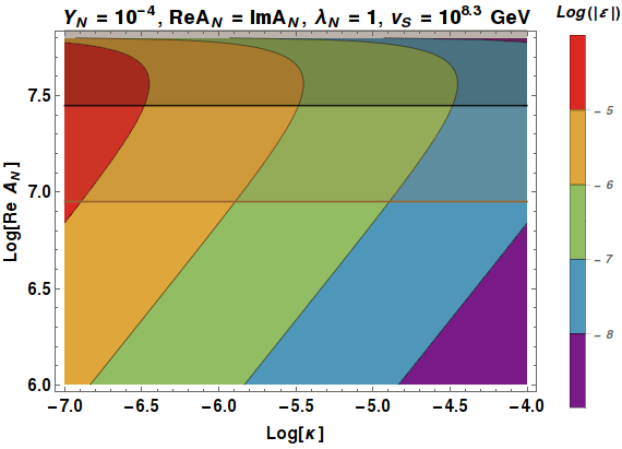
In Fig. 5 we take a complex with and vary and Re for GeV (left panel) and GeV (right panel). As can be seen from the left figure, we need large () to satisfy correct order of while ensuring that . However from the right panel, it is clear that sufficient CP asymmetry can be created even at leading order in without using thermal phase space factors.
We keep real in Fig. 6 and vary and for similar values of and as before. It’s clear that non-zero asymmetry can be created even with real as long as (). However compared to Fig. 5, we find that the bounds on and in Fig. 6 are stronger as there is much less parameter space available satisfying . Both Figs. 5 and 6 satisfy neutrino mass bounds and the conditions of .
V.2 Case 2:
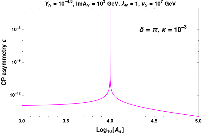
If the phase of the vev of is large, specially at , we get a resonance behaviour in at . In the limit of , the CP asymmetry parameter of Eq. (60) can be written as:
| (67) |
Eq. (67) also justifies assuming to derive the general constraints on the various parameters in Sec. IV. The behaviour of versus is shown in Fig. 7. For the plot, we take TeV. The values of the other relevant parameters are shown in the figure itself. Since , there is no contribution from the real part of in . This means that necessarily needs to be complex contrary to the case where is small. Without resonance, it was found in Sec. V.1 that needs to be several orders larger than for correct amount of . However, the resonance effect at mitigates this requirement allowing to be of the same order or smaller than .
VI Conclusion
We have presented a new mechanism for soft leptogenesis in the context of the NMSSM with a singlet RH neutrino superfield. Similar to soft leptogenesis in the MSSM, we also generate CP asymmetry at the tree-level owing to the CP violation occuring due to the difference between the mass and CP eigenstates similar to the or the systems. The difference lies in the fact that MSSM soft leptogenesis requires using thermal masses and phase space factors for boson and fermion final states without which there is no asymmetry. In the NMSSM where the singlet scalar takes a vev, an asymmetry can be generated even without any thermal phase space/mass corrections to the decay products. Further if there is spontaneous CP violation in the system with , lepton asymmetry can be created without using any other complex parameter. In the numerical analysis for small case, we considered the mass scale of the RH sneutrino to be GeV. We found that to generate sufficient asymmetry, one of the soft trilinear coupling needs to be GeV and . This also tells us that GeV. However, if , there occurs a resonance in the system which helps to obtain even with and the value of can be comparatively larger (). The mass of the RH sneutrino came out in the range GeV which lies below the cosmological gravitino overproduction bound of GeV Davidson and Ibarra 2002; Kawasaki et al. 2006; Khlopov and Linde 1984; Falomkin et al. 1984. This mass scale for the sneutrino (which depends on the vev of , ) in the NMSSM also could favour gravitational wave detection at LIGO Dev and Mazumdar 2016 provided a strong first order phase transition occurs in the scalar sector. It would be interesting to explore the flavor effects in the present scenario that we leave for a future study.
Acknowledgements
WA would like to acknowledge the support in the form of funding available from the Department of Atomic Energy, Government of India for the Neutrino Project at Harish-Chandra Research Institute (HRI). AK would like to thank Bharti Kindra for discussions on systems. AK and AKS acknowledge PRL for providing postdoctoral research fellowship.
References
- Tanabashi et al. (2018) M. Tanabashi et al. (Particle Data Group), Phys. Rev. D98, 030001 (2018).
- Fukugita and Yanagida (1986) M. Fukugita and T. Yanagida, Phys. Lett. B174, 45 (1986).
- Strumia (2006) A. Strumia, in Particle physics beyond the standard model. Proceedings, Summer School on Theoretical Physics, 84th Session, Les Houches, France, August 1-26, 2005 (2006) pp. 655–680, arXiv:hep-ph/0608347 [hep-ph] .
- Minkowski (1977) P. Minkowski, Phys. Lett. B67, 421 (1977).
- Mohapatra and Senjanovic (1980) R. N. Mohapatra and G. Senjanovic, Phys. Rev. Lett. 44, 912 (1980).
- Yanagida (1979) T. Yanagida, Proceedings: Workshop on the Unified Theories and the Baryon Number in the Universe: Tsukuba, Japan, February 13-14, 1979, Conf. Proc. C7902131, 95 (1979).
- Gell-Mann et al. (1979) M. Gell-Mann, P. Ramond, and R. Slansky, Supergravity Workshop Stony Brook, New York, September 27-28, 1979, Conf. Proc. C790927, 315 (1979), arXiv:1306.4669 [hep-th] .
- Glashow (1980) S. L. Glashow, Cargese Summer Institute: Quarks and Leptons Cargese, France, July 9-29, 1979, NATO Sci. Ser. B 61, 687 (1980).
- Schechter and Valle (1980) J. Schechter and J. W. F. Valle, Phys. Rev. D22, 2227 (1980).
- Kuzmin et al. (1985) V. A. Kuzmin, V. A. Rubakov, and M. E. Shaposhnikov, Phys. Lett. 155B, 36 (1985).
- Grossman et al. (2003) Y. Grossman, T. Kashti, Y. Nir, and E. Roulet, Phys. Rev. Lett. 91, 251801 (2003), arXiv:hep-ph/0307081 [hep-ph] .
- D’Ambrosio et al. (2003) G. D’Ambrosio, G. F. Giudice, and M. Raidal, Phys. Lett. B575, 75 (2003), arXiv:hep-ph/0308031 [hep-ph] .
- Fong et al. (2011a) C. S. Fong, M. C. Gonzalez-Garcia, and E. Nardi, Int. J. Mod. Phys. A26, 3491 (2011a), arXiv:1107.5312 [hep-ph] .
- Chen and Mahanthappa (2004) M.-C. Chen and K. T. Mahanthappa, Phys. Rev. D70, 113013 (2004), arXiv:hep-ph/0409096 [hep-ph] .
- Chun and Scopel (2006) E. J. Chun and S. Scopel, Phys. Lett. B636, 278 (2006), arXiv:hep-ph/0510170 [hep-ph] .
- Medina and Wagner (2006) A. D. Medina and C. E. M. Wagner, JHEP 12, 037 (2006), arXiv:hep-ph/0609052 [hep-ph] .
- Garayoa et al. (2007) J. Garayoa, M. C. Gonzalez-Garcia, and N. Rius, JHEP 02, 021 (2007), arXiv:hep-ph/0611311 [hep-ph] .
- Fong and Gonzalez-Garcia (2008) C. S. Fong and M. C. Gonzalez-Garcia, JHEP 06, 076 (2008), arXiv:0804.4471 [hep-ph] .
- Fong and Gonzalez-Garcia (2009) C. S. Fong and M. C. Gonzalez-Garcia, JHEP 03, 073 (2009), arXiv:0901.0008 [hep-ph] .
- Kajiyama et al. (2009) Y. Kajiyama, S. Khalil, and M. Raidal, Nucl. Phys. B820, 75 (2009), arXiv:0902.4405 [hep-ph] .
- Fong et al. (2010) C. S. Fong, M. C. Gonzalez-Garcia, E. Nardi, and J. Racker, JHEP 07, 001 (2010), arXiv:1004.5125 [hep-ph] .
- Hamaguchi and Yokozaki (2011) K. Hamaguchi and N. Yokozaki, Phys. Lett. B694, 398 (2011), arXiv:1007.3323 [hep-ph] .
- Fong et al. (2011b) C. S. Fong, M. C. Gonzalez-Garcia, and E. Nardi, JCAP 1102, 032 (2011b), arXiv:1012.1597 [hep-ph] .
- Kuismanen and Vilja (2013) H. Kuismanen and I. Vilja, Phys. Rev. D87, 015005 (2013), arXiv:1210.4335 [hep-ph] .
- Chung et al. (2005) D. J. H. Chung, L. L. Everett, G. L. Kane, S. F. King, J. D. Lykken, and L.-T. Wang, Phys. Rept. 407, 1 (2005), arXiv:hep-ph/0312378 [hep-ph] .
- (26) S. P. Martin, arXiv:hep-ph/9709356 [hep-ph] .
- Grossman et al. (2004) Y. Grossman, T. Kashti, Y. Nir, and E. Roulet, JHEP 11, 080 (2004), arXiv:hep-ph/0407063 [hep-ph] .
- Adhikari et al. (2015) R. Adhikari, A. Dasgupta, C. S. Fong, and R. Rangarajan, Phys. Rev. D91, 096001 (2015), arXiv:1501.06310 [hep-ph] .
- Kim and Nilles (1984) J. E. Kim and H. P. Nilles, Phys. Lett. 138B, 150 (1984).
- Ellwanger et al. (2010) U. Ellwanger, C. Hugonie, and A. M. Teixeira, Phys. Rept. 496, 1 (2010), arXiv:0910.1785 [hep-ph] .
- Maniatis (2010) M. Maniatis, Int. J. Mod. Phys. A25, 3505 (2010), arXiv:0906.0777 [hep-ph] .
- Grossman and Haber (1997) Y. Grossman and H. E. Haber, Phys. Rev. Lett. 78, 3438 (1997), arXiv:hep-ph/9702421 [hep-ph] .
- King (1998) S. F. King, Phys. Lett. B439, 350 (1998), arXiv:hep-ph/9806440 [hep-ph] .
- Kitano and Oda (2000) R. Kitano and K.-y. Oda, Phys. Rev. D61, 113001 (2000), arXiv:hep-ph/9911327 [hep-ph] .
- Das and Roy (2010) D. Das and S. Roy, Phys. Rev. D82, 035002 (2010), arXiv:1003.4381 [hep-ph] .
- Alanne et al. (2019) T. Alanne, T. Hugle, M. Platscher, and K. Schmitz, JCAP 1903, 037 (2019), arXiv:1812.04421 [hep-ph] .
- Esteban et al. (2017) I. Esteban, M. C. Gonzalez-Garcia, M. Maltoni, I. Martinez-Soler, and T. Schwetz, JHEP 01, 087 (2017), arXiv:1611.01514 [hep-ph] .
- de Salas et al. (2018) P. F. de Salas, D. V. Forero, C. A. Ternes, M. Tortola, and J. W. F. Valle, Phys. Lett. B782, 633 (2018), arXiv:1708.01186 [hep-ph] .
- Nir (2001) Y. Nir, in Heavy flavor physics: Theory and experimental results in heavy quark physics and CP violation. Proceedings, 55th Scottish Universities Summer School in Physics, SUSSP 2001, St. Andrews, UK, August 7-23, 2001 (2001) pp. 147–200, arXiv:hep-ph/0109090 [hep-ph] .
- Aghanim et al. (2018) N. Aghanim et al. (Planck), (2018), arXiv:1807.06209 [astro-ph.CO] .
- Huitu et al. (2012) K. Huitu, J. Laamanen, L. Leinonen, S. K. Rai, and T. Ruppell, JHEP 11, 129 (2012), arXiv:1209.6302 [hep-ph] .
- King et al. (2015) S. F. King, M. Muhlleitner, R. Nevzorov, and K. Walz, Nucl. Phys. B901, 526 (2015), arXiv:1508.03255 [hep-ph] .
- Buchmuller et al. (2005) W. Buchmuller, P. Di Bari, and M. Plumacher, Annals Phys. 315, 305 (2005), arXiv:hep-ph/0401240 [hep-ph] .
- Garayoa et al. (2009) J. Garayoa, S. Pastor, T. Pinto, N. Rius, and O. Vives, JCAP 0909, 035 (2009), arXiv:0905.4834 [hep-ph] .
- Hahn-Woernle et al. (2009) F. Hahn-Woernle, M. Plumacher, and Y. Y. Y. Wong, JCAP 0908, 028 (2009), arXiv:0907.0205 [hep-ph] .
- Davidson and Ibarra (2002) S. Davidson and A. Ibarra, Phys. Lett. B535, 25 (2002), arXiv:hep-ph/0202239 [hep-ph] .
- Kawasaki et al. (2006) M. Kawasaki, F. Takahashi, and T. T. Yanagida, Phys. Rev. D74, 043519 (2006), arXiv:hep-ph/0605297 [hep-ph] .
- Khlopov and Linde (1984) M. Yu. Khlopov and A. D. Linde, Phys. Lett. 138B, 265 (1984).
- Falomkin et al. (1984) I. V. Falomkin, G. B. Pontecorvo, M. G. Sapozhnikov, M. Y. Khlopov, F. Balestra, and G. Piragino, Il Nuovo Cimento A (1965-1970) 79, 193 (1984).
- Dev and Mazumdar (2016) P. S. B. Dev and A. Mazumdar, Phys. Rev. D93, 104001 (2016), arXiv:1602.04203 [hep-ph] .