Reflection matrix approach for quantitative imaging of scattering media
Abstract
We present a physically intuitive matrix approach for wave imaging and characterization in scattering media. The experimental proof-of-concept is performed with ultrasonic waves, but this approach can be applied to any field of wave physics for which multi-element technology is available. The concept is that focused beamforming enables the synthesis, in transmit and receive, of an array of virtual transducers which map the entire medium to be imaged. The inter-element responses of this virtual array form a focused reflection matrix from which spatial maps of various characteristics of the propagating wave can be retrieved. Here we demonstrate: (i) a local focusing criterion that enables the image quality and the wave velocity to be evaluated everywhere inside the medium, including in random speckle, and (ii) an highly resolved spatial mapping of the prevalence of multiple scattering, which constitutes a new and unique contrast for ultrasonic imaging. The approach is demonstrated for a controllable phantom system, and for in vivo imaging of the human abdomen. More generally, this matrix approach opens an original and powerful route for quantitative imaging in wave physics.
I Introduction
In wave imaging, we aim to characterize an unknown environment by actively illuminating a region and recording the reflected waves. Inhomogeneities generate back-scattered echoes that can be used to image the local reflectivity of the medium. This is the principle of, for example, ultrasound imaging Szabo 2004, optical coherence tomography for light Drexler and Fujimoto 2008, radar for electromagnetic waves Bamler and Hartl 1998 or reflection seismology in geophysics Yilmaz 2008. This approach, however, rests on the assumption of a homogeneous medium between the probe and target. Large-scale fluctuations of the wave velocity in the medium can result in wavefront distortion (aberration) and a loss of resolution in the subsequent reflectivity image. Smaller-scale inhomogeneities with high concentration and/or scattering strength can induce multiple scattering events which can strongly degrade image contrast. In the past, numerous methods such as adaptive focusing have been implemented to correct for these fundamental issues in reflectivity imaging Roddier 1999; Booth 2007; O’Donnell and Flax 1988; Mallart and Fink 1994. However, such methods are largely ineffective in situations where the focus quality inside the medium can not be determined. An extremely common example of this situation for ultrasound imaging is the presence of speckle, the signal resulting from an incoherent sum of echoes due to randomly distributed unresolved scatterers. Speckle often dominates medical ultrasound images, making adaptive focusing difficult.
Alternately, one can try to exploit effects which are detrimental to reflectivity imaging (such as distortion and scattering) to create different imaging modalities. In the ballistic regime (where single scattering dominates), the refractive index can be estimated by analyzing the distortion undergone by the wave as it passes through the medium. This is the principle of quantitative phase imaging Park et al. 2018 in optics and computed tomography Kak and Slaney 2001 in ultrasound imaging. Most such approaches, however, require a transmission configuration, which is not practical for thick scattering media, and which is impossible for most in-vivo or in-situ applications in which only one side of the medium is accessible. In reflection, recent work has leveraged the relationship between the speed of sound and wavefront distortion to improve aberrated images Ali and Dahl 2018; Rau et al. 2019; Chau et al. 2019 or to measure Jaeger et al. 2015a. Based on comparisons between the spatial or temporal coherence between emitted and detected signals at a transducer array, such approaches are promising for the correction of wavefront distortions when single scattering dominates.
In the multiple scattering regime, optical diffuse tomography Durduran et al. 2010 is a well-established technique to build a map of transport parameters. However, the spatial resolution of the resulting image is poor as it scales with imaging depth. Moreover, this approach assumes a purely multiple scattering medium, which does not exist in practice. A single scattering contribution always exists, and is furthermore typically predominant in ultrasound imaging. To evaluate the validity of such images, a local (spatially-resolved) multiple scattering rate would be a valuable observable, but is not accessible with state-of-the-art methods.
Recently, a reflection matrix approach to wave imaging was developed with the goals of: (i) processing the huge amount of data that can now be recorded with multi-element arrays Montaldo et al. 2009; Mosk and van Putten 2010; Provost et al. 2014, and (ii) optimizing aberration correction Varslot et al. 2004; Robert and Fink 2008; Kang et al. 2017; Badon et al. 2019 and multiple scattering removal Aubry and Derode 2009; Aubry and Derode 2011; Kang et al. 2015; Badon et al. 2016a in post-processing. Such matrix approaches provide access to much more information than is available with conventional imaging techniques. Their recent successes suggest that access to detailed information on aberration and multiple scattering could be capitalized upon for more accurate characterization of strongly heterogeneous media. In this paper, we introduce a universal and non-invasive matrix approach for new quantitative imaging modes in reflection.
Our method is based on the projection of the reflection matrix into a focused basis Badon et al. 2016a; Blondel et al. 2018. This focused reflection matrix can be thought of as a matrix of impulse responses between virtual transducers located inside the medium Robert and Fink 2008. These virtual transducers are created via numerical simulation of wave focusing, i.e. combining all of the backscattered echoes in such as way as to mimic focusing at a set of focal points that spans the entire medium, in both transmit and receive. While each pixel of a confocal image is associated with the same virtual transducer at emission and reception, the focused reflection matrix also contains the cross-talks between each pixel of the image, and thus holds much more information than a conventional image. Importantly, this matrix allows to probe the input-output point spread function (PSF) in the vicinity of each pixel even in speckle. A local PSF in reflection is a particularly relevant observable since it allows a local quantification of the contribution of aberration and multiple scattering to the image. More precisely, we demonstrate here the mapping of: (i) a local focusing criterion that can then be used as a guide star for wave velocity tomography Jaeger et al. 2015b; Imbault et al. 2017; Stähli et al. 2019 in the medium, and (ii) a spatially-resolved multiple scattering rate which paves the way towards local measurements of wave transport parameters Aubry et al. 2008; Aubry and Derode 2011; Mohanty et al. 2017 such as the absorption length and the scattering mean free path (the mean distance between two successive scattering events). Not only are these parameters quantitative markers for biomedical diagnosis in ultrasound imaging Suzuki et al. 1992; Sasso et al. 2010; Bamber and Hill 1981; Bamber et al. 1981; Chen et al. 1987; Duck 1990 and optical microscopy Durduran et al. 2010, but they are also important observables for non-destructive evaluation Schurr et al. 2011; Shajahan et al. 2014; Zhang et al. 2016 and geophysics Sato et al. 2012; Chaput et al. 2015; Mayor et al. 2018. In this paper, we present the principle and first experimental proofs of concept of our approach in the context of medical ultrasound imaging. However, the concept can be extended to any field of wave physics for which multi-element technology (multiple sources/receivers which can emit/detect independently from one another) is available.
The paper is structured as follows: Section II presents the concept and theoretical foundations of the focused reflection matrix. Then, experiments on a tissue-mimicking phantom are used to demonstrate proofs of concept in Section III for spatial mapping of the quality of focus and speed of sound, and in Section IV for spatial mapping of multiple scattering. Perspectives for each are discussed. In Section V, these techniques are applied for in vivo quantitative imaging of the human liver. Finally, Section VI presents conclusions and general perspectives.
II Reflection Matrix approach
II.1 Experimental measurement
The sample under investigation is a tissue-mimicking phantom composed of subresolution scatterers which generate ultrasonic speckle characteristic of human tissue [Fig. 1(a)]. The system also contains point-like specular targets are placed at regular intervals, and at larger depths, two sections of hyperechoic cylinders, each containing a different (higher) density of unresolved scatterers. A 20 mm-thick layer of bovine tissue is placed on top of the phantom and acts as both an aberrating and scattering layer. This experiment mimics the situation of in-vivo liver imaging in which layers of fat and muscle tissues generate strong aberration and scattering at shallow depths. We acquire the acoustic reflection matrix experimentally using a linear ultrasonic transducer array placed in direct contact with the sample [Fig. 1(a)]. The simplest acquisition sequence is to emit with one element at a time, and for each emission record with all elements the time-dependent field reflected back from the medium. This canonical basis was first used to describe the so-called time-reversal operator Prada and Fink 1994, and is now commonly used in non destructive testing where it is referred to as the full matrix capture sequence Holmes et al. 2005. A matrix acquired in this way can be written mathematically as , where is the position of elements along the array, ‘in’ denotes transmission, and ‘out’ denotes reception. Alternately, the response matrix can be acquired using beamforming (emitting and/or receiving with all elements in concert with appropriate time delays applied to each element) to form, for example, focused beams as in the conventional B-mode Szabo 2004 or plane waves for high frame rate imaging Montaldo et al. 2009. To demonstrate the compatibility of our method with state-of-the-art medical technology, our data was acquired using plane-wave beamforming in emission and recording with individual elements in reception.

The experimental procedure is described in detail in Appendix A. A set of plane waves is used to probe the medium of interest. For each plane wave emitted with an incident angle , the time-dependent reflected wavefield is recorded by the transducers. The corresponding signals are stored in a reflection matrix [Fig. 1(a)]. An ultrasound image can be formed by coherently summing the recorded echoes coming from each focal point , which then acts as a virtual detector inside the medium. In practice, this is done by applying appropriate time delays to the recorded signals Montaldo et al. 2009. The images obtained for each incident plane wave are then summed up coherently and result in a final compounded image with upgraded contrast. This last operation generates a posteriori a synthetic focusing (i.e. a virtual source) on each focal point. The compounded image is thus equivalent to a confocal image that would be obtained by focusing waves on the same point in both the transmit and receive modes.
II.2 Monochromatic focused reflection matrix
We now show how all of the aforementioned imaging steps can be rewritten under a matrix formalism. The reflection matrix can actually be defined in general as containing responses between one or two mathematical bases. The bases implicated in this work are: (i) the recording basis which here corresponds to the transducer array, (ii) the illumination basis which is composed of the incident plane waves, and (iii) the focused basis in which the ultrasound image is built. In the frequency domain, simple matrix products allow ultrasonic data to be easily projected from the illumination and recording bases to the focused basis where local information on the medium proprieties can be extracted.
Consequently, a temporal Fourier transform should be first applied to the experimentally acquired reflection matrix to obtain , where is the angular frequency of the waves. The matrix can be expressed as follows:
| (1) |
where the matrix , defined in the focused basis, describes the scattering process inside the medium. In the single scattering regime, is diagonal and its elements correspond to the medium reflectivity . is the transmission matrix between the plane wave and focused bases. Each column of this matrix describes the incident wavefield induced inside the sample by a plane wave of angle . is the Green’s matrix between the transducer and focused bases. Each line of this matrix corresponds to the wavefront that would be recorded by the array of transducers along vector if a point source was introduced at a point inside the sample.
The holy grail for imaging is to have access to these transmission and Green’s matrices. Their inversion, pseudo-inversion, or more simply their phase conjugation can enable the reconstruction of a reliable image of the scattering medium, thereby overcoming the aberration and multiple scattering effects induced by the medium itself. However, direct measurement of the transmission and Green’s matrices and would require the introduction of sensors inside the medium, and therefore these matrices are not accessible in most imaging configurations. Instead, sound propagation from the plane-wave or transducer bases to the focal points is usually modelled assuming a homogeneous speed of sound . In this case, the elements of the corresponding free-space transmission matrix are given by
| (2) |
where and describe the coordinates of in the lateral and axial directions, respectively [Fig. 1(a)], and is the wave number. The elements of the free-space Green’s matrix are the 2D Green’s functions between the transducers and the focal points Watanabe 2014
| (3) |
where is the Hankel function of the first kind. and can be used to project the reflection matrix into the focused basis. Based on Kirchhoff’s diffraction theory Goodman 1996, such a double focusing operation can be written as the following matrix product
| (4) |
where the symbol and stand for phase conjugate and transpose conjugate, respectively. The matrices and contain the phase-conjugated wavefronts that should be applied at emission and reception in order to project the reflection matrix into the focused basis both at input () and output (). Equation (4) thus mimics focused beamforming in post-processing in both emission and reception. Each coefficient of is the impulse response between a virtual source at point and a virtual detector at [Fig. 1(c)].
The aberration issue in imaging can be investigated by expressing the matrix mathematically using Eqs. (1) and (4):
| (5) |
where
| (6) |
and
| (7) |
are the input and output focusing matrices, respectively [Fig. 1(b)]. Each column of and corresponds to the transmit and receive PSFs, i.e. the spatial amplitude distribution of the input and output focal spots. Their support defines the characteristic size of each virtual source at and detector at [Fig. 1(b)]. In the absence of aberration, the transverse and axial dimension of these focal spots, and , are only limited by diffraction Born and Wolf 2003:
| (8) |
where is the maximum angle of wave illumination or collection by the array and the wavelength. In the presence of aberration, i.e. if the velocity model is inaccurate, there is a mismatch between the transmission and Green’s matrices, and , and their free-space counterparts, and . The focusing matrices, and , are far from being diagonal [Eqs.(6)-(7)]. The corresponding PSFs are strongly degraded and the virtual transducers can overlap significantly. A better model of wave propagation is thus needed to overcome aberrations and restore diffraction-limited PSFs. In Sec. III.1, we will show how a multilayer model can be used to reach a better estimate of and in the experimental configuration depicted in Fig. 1(a).
II.3 Broadband focused reflection matrix

For broadband imaging, we can restrict our study to pairs of virtual transducers, and , located at the same depth . Furthermore, an inverse Fourier transform of the corresponding sub-matrices should be performed in order to recover the excellent axial resolution of ultrasound images. For direct imaging, only echoes at the ballistic time ( in the focused basis) are of interest. This ballistic time gating can be performed via a coherent sum of over the frequency bandwidth . A broadband focused reflection matrix is thus obtained at each depth :
| (9) |
where and is the central frequency. Each element of contains the signal that would be recorded by a virtual transducer located at just after a virtual source at emits a pulse of length at the central frequency . The broadband focusing operation of Eq. (9) gives virtual transducers which now have a greatly reduced axial dimension [Fig. 1(c)].
Figures 2(a) and (b) display at the bovine tissue/phantom interface ( mm) and in the phantom ( mm), respectively. In both cases, most of the signal is concentrated around the diagonal. This indicates that single scattering dominates at these depths Badon et al. 2016a, since a singly-scattered wavefield can only originate from the point which was illuminated by the incident focal spot. In fact, the elements of which obey hold the information which would be obtained via multifocus (or confocal) imaging, in which transmit and receive focusing are performed at the same location for each point in the medium. A line of the ultrasound image can thus be directly deduced from the diagonal elements of , computed at each depth:
| (10) |
The corresponding image is displayed in Fig. 2(c). It is equivalent to the coherent compounding image computed via delay-and-sum beamforming of the same data set Montaldo et al. 2009, constituting a validation of our matrix approach for imaging.
Interestingly, the matrix contains much more information than a single ultrasound image. In particular, focusing quality can be assessed by means of the off-diagonal elements of . To understand why this is, shall be expressed theoretically. To that aim, a time-gated version of Eq. (5) can be derived:
| (11) |
where , and are the time-gated sub-matrices of [Eq. (6)], [Eq. (1)] and [Eq. (7)] at depth and central frequency . In the single scattering regime and for spatially- and frequency-invariant aberration, the previous equation can be rewritten in terms of matrix coefficients as follows:
| (12) | |||||
This last equation confirms that the diagonal coefficients of , i.e. a line of the ultrasound image, result from a convolution between the sample reflectivity and the confocal PSF . As we will see, access to the off-diagonal elements of will allow our analysis of the experimental data to go far beyond a simple image of the reflectivity. In particular, off-diagonal elements can be used to extract the input-output PSF in the vicinity of each focal point, which will lead to a local quantification of the focusing quality.
III Local focusing criterion
In this section, we detail how an investigation of the off-diagonal points in can directly provide a focusing quality criterion for any pixel of the ultrasound image. To that aim, the relevant observable is the mean intensity profile along each antidiagonal of :
| (13) |
where denotes an average over the pairs of points and which share the same midpoint , and is the relative position between those two points. We term the common-midpoint intensity profile. Whereas [Eq. (10)] only contains the confocal intensity response from an impulse at point , is a measure of the spatially-dependent intensity response to an impulse at . This means that whatever the scattering properties of the sample, allows an estimation of the input-output PSFs. However, its theoretical expression differs slightly depending on the characteristic length scale of the reflectivity at the ballistic depth and the typical width of the input and output focal spots.
In the specular scattering regime [, see Fig. 2(a)], the common-midpoint intensity is directly proportional to the convolution between the coherent input and output PSFs, and (see Appendix B):
| (14) |
where the symbol stands for convolution. However, in ultrasound imaging, scattering is more often due to a random distribution of unresolved scatterers. In this speckle regime [, see Fig. 2(b)], the common midpoint intensity is directly proportional to the convolution between the incoherent input and output PSFs, and (see Appendix B):
| (15) |
The ensemble average in Eq. 15 implies access to several realizations of disorder for each image, which is often not possible for most applications. In the absence of multiple realizations, a spatial average over a few resolution cells is required to smooth intensity fluctuations due to the random reflectivity of the sample while keeping a satisfactory spatial resolution. To do so, a spatially averaged intensity profile is computed at each point of the field of view, such that
| (16) |
where the symbol denotes an average over the set of focusing points contained in an area centered on . The compromise between intensity fluctuations and spatial resolution guided our choice of a 7.5 mm-diameter disk for .
Whatever the scattering regime, the averaged common-midpoint intensity profile is a direct indicator of the focusing resolution at each point of the medium. One can then build a local focusing parameter
| (17) |
where the input-output focusing resolution is defined as the full width at half maximum (FWHM) of , and is a reference value based on the theoretical diffraction limit for a homogeneous medium. This parameter is bounded between 0 (, bad focusing) and 1 (, perfect focusing). is the equivalent in the focused basis of the coherence or focusing factor originally introduced by Mallart and Fink Mallart and Fink 1994 in the transducer basis. The definition of a focusing parameter in the focused basis offers an important advantage in that the wave focusing quality and the image resolution can now be probed locally.
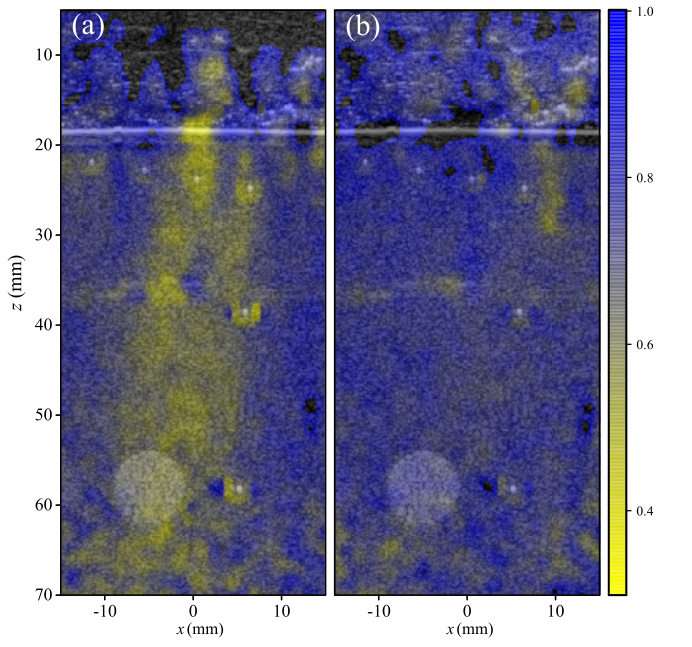
Figure 3(a) shows the focusing criterion calculated for the bovine tissue/phantom system [corresponding to the reflectivity image of Fig. 2(c)]. The reference resolution has been computed under a speckle scattering hypothesis [Eq. (30)]. The poor quality of focus over a large part of the image can be attributed to the fact that the presence of the bovine tissue layer was not taken into account in our (homogeneous) model of the system [Eqs. (2) – (4)]. Fortunately, as discussed in the following section, the focused reflection matrix approach enables the determination of a more accurate model for this a priori unknown medium.
III.1 Wave velocity mapping
The ability to locally probe the focus quality offers enormous advantages for local characterization of heterogeneous media, in particular for a quantitative mapping of their refractive index, or more specifically, as shown in the following, the speed of sound.
We begin by observing the focusing criterion at the bovine tissue-phantom interface as a function of the wave velocity assumed in the bovine tissue. The result is displayed in Fig. 2(e). The corresponding focusing criterion is optimized for m/s. Fig. 2(g) shows the reflection matrix obtained by considering this optimized wave velocity. The comparison with the original matrix displayed in Fig. 2(a) shows a narrowing of the input-output PSFs along the antidiagonal of ; the focusing resolution is now much closer to the diffraction limit due to the use of the optimized .
This approach works for a reasonably homogeneous medium (the tissue layer). However, our assumption of a homogeneous wave velocity model does not conform to the bi-layer system under experimental investigation [Fig. 1(a)]. To probe more deeply into the system, we extend our approach to model a multilayer medium. Using the ultrasound image [Fig. 2(c)] as an approximate guide, we define two layers: one at mm with our measured , and a second for depths below mm with unknown wave velocity . New transmission and Green’s matrices, and , are computed using this two-layer wave velocity model. A new reflection matrix is then built via
| (18) |
Figure 2(h) displays at depth mm. The corresponding focusing criterion , averaged over the full width of the image and a mm range of depths, is shown as a function of the phantom speed of sound hypothesis in Fig. 2(e). The optimization of yields a quantitative measurement of the speed of sound in the phantom: m/s.
To build an entire profile of wave velocity throughout the medium, the optimization is repeated for each depth. The resulting depth-dependent velocity estimate is shown in Fig. 2(d). The presence of two layers can be clearly seen, corresponding to the bovine tissue with mean wave velocity m/s ( mm), and the phantom with m/s ( mm). These values are in excellent agreement with the manufacturer’s specification for the phantom ( m/s) and the speed of sound estimated from the travel time of the pulse reflected off of the tissue/phantom interface ( m/s). At depths just below the interface between the two layers, the measurement of appears to be less precise. This effect can be explained by the fact that the measurement error on the wave velocity scales as the inverse of , the depth of the focal plane from the phantom surface [see Appendix D, Eq. 39]:
| (19) |
with . As the precision with which the focusing criterion can be measured is [see Fig. 2(e)], a precision of m/s for the wave velocity in the second layer (the phantom) will only be reached for mm. This value is in qualitative agreement with the axial resolution of the wave velocity profile displayed in Fig. 2(d).
Figure 2(f) shows the ultrasound image deduced from the confocal elements of . Compared with the homogeneous model [Fig. 2(c)], it can be seen by eye that the two-layer model slightly improves the imaging of bright targets, but that there is no clear difference in areas of speckle. However, the result for after optimization with the two-layer model shows that a significant improvement in quality of focus has been obtained with the two-layer model (Fig. 3). The significance of this result is that, in regions of speckle, is far more sensitive than image brightness to the quality of focus and speed of sound. As most state of the art methods for speed of sound measurement are based on image brightness Mehta et al. 2008; Dasarathy et al. 2009; Zubajlo et al. 2018, thus constitutes an important new metric for speed of sound measurement in heterogeneous media.
III.2 Discussion
The study of the focused reflection matrix yields a quantitative, local focusing criterion. To our knowledge, this is the first demonstration of such spatial mapping of focus quality (e.g. Fig. 3). While this information is useful to evaluate the reliability of the associated ultrasound images, it has even more potentional for therapeutic ultrasound methods which rely on precisely focused beams for energy delivery, such as high-intensity focused ultrasound (HIFU) Kennedy 2005, ultrasound neuromodulation Blackmore et al. 2019, and histotripsy Macoskey et al. 2018.
Going further, the local focusing parameter constitutes a sensitive guide star to map the wave velocity of an inhomogeneous scattering medium. The perspective of this work will be to go beyond a depth profile of the wave velocity to map its variations in 2D (1D probe) or 3D (2D array). In this respect, we shall mention the recent work of Jaeger et al. Jaeger et al. 2015b; Stähli et al. 2019 that investigated the local phase change at a point when changing the transmit beam steering angle. Looking at this local phase change under a matrix formalism would be a way to make the best of the two approaches. An inverse problem would then have to be solved to retrieve a map of the local phase velocity Jaeger et al. 2015b; Stähli et al. 2019. Again, a matrix formalism could be relevant to optimize this inversion.
In the same context, we would also like to mention the work of Imbault et al. Imbault et al. 2017 that investigated the correlations of the reflected wavefield in the transducer basis for a set of focused illuminations. Combined with a time reversal process consisting in iteratively synthesizing a virtual reflector in speckle Montaldo et al. 2011, the wave speed was measured by maximizing a focusing criterion based on the spatial correlations of the reflected wavefield Mallart and Fink 1994. The downside of this approach is that the construction of the virtual reflector requires that the focusing algorithm be iterated several times before the guide-star becomes point-like. Moreover, the whole process should be both averaged and repeated over each isoplanatic patch of the image Dahl et al. 2005, which limits the spatial resolution and the practicability of such a measurement.
Inspired by previous works Mallart and Fink 1994; Robert and Fink 2008; Montaldo et al. 2011; Imbault et al. 2017, novel potential applications can be imagined for . It could, for instance, be used as a guide star for a matrix correction of aberration. Based on its maximization, the goal would be to converge towards the best estimators of the transmission matrices and . An inversion or pseudo-inversion of these matrices would then lead to an optimized image whose resolution would be only limited by diffraction.
The developments presented thus far have been based on a single scattering assumption. However, multiple scattering is often far from being negligible in real-life ultrasound imaging, whether it be for example in soft human tissues Aubry and Derode 2011 or coarse-grain materials Shajahan et al. 2014. In the following, we show how the reflection matrix approach suggests a solution for the multiple scattering problem, and how it can furthermore be exploited to create a new contrast for ultrasound imaging.
IV Multiple scattering
In the previous sections, we developed a local focusing criterion by considering the near-confocal elements of . We now turn our attention to the points which are farther from the confocal elements, i.e. for which . Figure 4(a) shows at a depth of mm. Signal can clearly be seen at points far from the diagonal. Because each matrix is investigated at the ballistic time (), the only possible physical origin of echoes between distant virtual transducers is the existence of multiple scattering paths occurring at depths shallower than the focal depth, as sketched in Fig. 4(b). In this section, we will see that a significant amount of multiple scattering takes place in our bovine tissue/phantom system. Signal from such multiple scattering processes has traditionally been seen as a nightmare for classical wave imaging, as it presents as an incoherent background which can greatly degrade image contrast. However, because they are extremely sensitive to the micro-architecture of the medium, multiply scattered waves can be a valuable tool for the characterization of scattering media Aubry et al. 2008; Aubry and Derode 2011; Mohanty et al. 2017. In the following, we show how our matrix approach enables the measurement of a local multiple scattering rate for each pixel of the ultrasound image. This multiple scattering rate can be directly related to the concentration of scatterers, paving the way towards a novel contrast for ultrasound imaging.

IV.1 Multiple scattering in the focused basis
For our experimental configuration, multiple scattering can be investigated by examining the averaged spatial intensity profiles [Eq. (16)]. Each intensity profile is composed of three contributions:
- 1.
The single scattering component, . Signals from single scattering mainly lie along the near-confocal elements of []. This is the contribution that has been investigated in the previous sections.
- 2.
The multiple scattering component, . This contribution can be split into two terms: An incoherent part which corresponds to interferences between waves taking different paths through the medium, and a coherent part which corresponds to the interference of waves with their reciprocal counterparts [see the blue and red paths in Fig. 4(b). Referred to as coherent backscattering (CBS), this interference phenomenon results in an enhancement (of around two) in intensity at exact backscattering. Originally discovered in the plane wave basis Kuga and Ishimaru 1984; Van Albada and Lagendijk 1985; Wolf and Maret 1985; Akkermans et al. 1988, this phenomenon also occurs in a point-to-point basis, whether the points be real sensors Bayer and Niederdränk 1993; Tourin et al. 1997; Larose et al. 2004 or created via focused beamforming Aubry and Derode 2007; Aubry et al. 2008. In the point-to-point basis, contributions from multiple scattering give to the backscattered intensity profile the following shape: a narrow, steep peak (the CBS peak) in the vicinity of the source location [], which sits on top of a wider pedestal (the incoherent contribution).
- 3.
Electronic noise, . These contribution can decrease the contrast of an ultrasound image in the same way as . Noise contributes to a roughly constant background level to the backscattered intensity profiles .

To estimate the level of each contribution, the relevant observables are the mean confocal intensity () and off-diagonal intensity () of . The confocal intensity is given by
| (20) |
where the factor of accounts for the CBS enhancement of the multiple scattering intensity at the source location. is the sum of the multiple scattering incoherent background and of the additive noise component:
| (21) |
where indicates an average over off-diagonal elements which obey . This average constitutes an average over several realizations of disorder, which is necessary to suppress the fluctuations from constructive and destructive interference between the various possible multiple scattering paths through the sample. Figure 5(a) shows three examples of normalized intensity profiles . Each profile has been averaged over a different zone of the ultrasound image [Fig. 5(c)]: green and blue curves (solid and dotted rectangles) correspond to zones situated respectively above and below the bright speckle disk. It is clear that the incoherent background is higher in the deeper (blue) zone, suggesting that multiple scattering is greatly enhanced behind the reflective object. Surprisingly, the incoherent background is far from being negligible in the red zone at shallower depths (dashed line rectangle).
To investigate these phenomena further, we define two new observables: (1) the multiple-to-single scattering ratio
| (22) |
and (2) the multiple scattering-to-noise ratio,
| (23) |
To calculate these quantities, it is necessary to be able to distinguish between , , and .
IV.2 Coherent backscattering as a direct probe of spatial reciprocity
Discrimination between and can be achieved by exploiting the spatial reciprocity of propagating waves in a linear medium. While the multiple scattering contribution gives rise to a random but symmetric reflection matrix Badon et al. 2016a; Blondel et al. 2018, additive noise is fully random. Thus, the symmetry of gives us a tool to determine the relative weight between noise and multiple scattering in the incoherent background of .
An elegant approach to probe spatial reciprocity is the measurement of the CBS effect in the plane-wave basis (the far-field). The CBS effect can be observed by measuring the average backscattered intensity as a function of the angle between the incident and reflected waves. In the presence of multiple scattering, this profile displays a flat plateau (the incoherent background), on top of which sits a CBS cone centered around the exact backscattering angle . The cone is solely due to constructive interference from waves following reciprocal paths inside the sample [Fig. 5(b), inset]. Thus, CBS in the far-field is a direct probe of spatial reciprocity in the focused basis Aubry and Derode 2007; Aubry et al. 2008.
Appendix D describes how to eliminate the single scattering contribution and extract a far-field intensity profile for the area surrounding each focusing point . In Fig. 5(b), normalized intensity profiles are shown for the three areas highlighted in Fig. 5(c). For each area, a CBS cone is clearly visible, showing that the experimental data contain contributions from multiple scattering. Just as with the CBS peak in the focused basis [Fig. 5(a)], the highest amount of multiple scattering is observed for the red zone at shallow depths.
To estimate the relative weight of the noise and multiple scattering contributions, we examine the mean intensity for two cases: (1) at exact backscattering
| (24) |
and (2) at angles away from the CBS peak [Fig. 5(d)]
| (25) |
where is the width of the CBS peak and indicates an average over all angles which obey . The enhancement factor of the CBS peak is given by
| (26) |
can have values ranging from to ; it is at a minimum when and a maximum when all backscattered signal originates from multiple scattering.
IV.3 Maps of multiple scattering rates
The multiple scattering-to-noise ratio [Eq. 23] can be expressed as a function of the enhancement factor by injecting Eqs. 24 and 25 into Eq. 26 :
| (27) |
The multiple-to-single scattering ratio [Eq. 22] can be derived by injecting the last equation into Eqs. 20 and 21
| (28) |
Figures 5 (d) and (e) show experimental results for and , respectively, superimposed onto the original ultrasound image. Both of these maps constitute new contrasts which are complementary to the reflectivity maps produced by conventional ultrasound imaging. To begin with, can be used as an indicator of the reliability of a reflectivity image [such as that in Fig. 5(c)]. Because the single-to-multiple scattering ratio is a direct indicator of the validity of the single-scattering (Born) approximation, the reliability of the ultrasound image should scale as the inverse of . An interesting example is displayed in Fig. 5(d) at a depth of mm (white solid rounded rectangle), where a high multiple-to-single scattering rate is observed. This abrupt increase of can be accounted for by double reflection events between the probe and the tissue-phantom interface. We can thus conclude that the structures that seem to emerge in Fig. 5(c) at the same depth are in fact artifacts due to multiple reflections.
With respect to the quantification of multiple scattering, the parameter seems to be particularly relevant. The areas in Fig. 5(e) highlighted by dashed lines exhibit a strong and extended multiple scattering background. While deeper speckle regions with low scatterer density exhibit a low scattering rate, the bright speckle area in the phantom ( mm, white dashed-dotted circle) contains a sufficient concentration of scatterers to generate multiple scattering events. At shallower depths, high amounts of multiple scattering can be attributed to several small structures indicated by white arrows in Fig. 5(c): (i) two regions in the bovine tissue layer contain air bubbles that generate resonant scattering, thereby inducing a strong multiple scattering ‘tail’ behind them; (ii) a set of bright targets close to each other give rise to strong multiply-scattered echoes at depth 50 mm. Figure 5(e) thus demonstrates how the parameter can provide a highly contrasted map of the multiple scattering rate – a quantity which is directly related to the density of scatterers Sheng 2006.
Finally, use of both maps for the interpretation of specific regions can be instructive. While it could be suggested that the enhancement of [Fig. 5(d)] at the upper dotted lines is due to acoustic shadowing (a decrease in ), indicates that the level of multiple scattering dominates above noise [Fig. 5(e)]. Thus, one can conclude that multiple scattering is truly increased in this area. On the contrary, the area on the top left of the phantom shows a large increase of [Fig. 5(d)] but a weak multiple scattering-to-noise ratio [Fig. 5(e)]. Hence, the high value of is here induced by the acoustic shadow of the bovine tissue layer upstream.
An important technical note is that the study of spatial reciprocity in the reflection matrix requires in principle that the bases of reception and emission be identical. Because this is not the case for our experimental measurements, this tends to slightly underestimate .
Relatedly, here we have employed the CBS effect to probe spatial reciprocity, but an equivalent measurement can be performed directly in the focused basis by computing correlations between symmetric elements of .
IV.4 Discussion
The maps of and help to provide an overall assessment of the factors impacting image quality. For instance, they can be used to explain the apparent poor focus quality in some areas of Fig. 3(b), which appear even after correction for wavefront distortion. The compensation for an incorrect hypothesis for does not compensate for the effect of multiple scattering or reflections [e.g. in the highlighted areas of Fig. 5(e)]. Thus, the multiple scattering rates combined with the measurement of provide a sensitive local mapping of the heterogeneities in the medium which includes both small- and large-scale variations of the refractive index. In this context, we would like to mention the recent work of Velichko Velichko 2019, which measures a quantity similar to as a function of depth and frequency. While noise is not treated separately from multiple scattering, their results emphasize the clear relation between local measurements of multiple scattering and the reliability of ultrasound images. Integration of our focused reflection matrix approach [Eq. (11)] could improve their axial resolution, and help extend their analysis to 2D spatial mapping.
Beyond image reliability, the maps displayed in Fig. 5(d,e) provide a great deal of quantitative information about the system under investigation. Because is calculated from the off-diagonal elements of , it contains only negligible contributions from single scattering, and thus constitutes an interesting new contrast for imaging which is much more sensitive to the microstructure of the medium than it is to its reflectivity. Conversely, because is independent of noise, it can constitute a useful biomarker for medical imaging deep inside tissue, and a potentially valuable tool for future research seeking to characterize multiple scattering media, even at large depths where becomes important.
The perspective of this work will be to extract from quantitative maps of scattering parameters such as the elastic mean free path or the absorption length Shajahan et al. 2014; Aubry and Derode 2011, and transport parameters such as the transport mean free path Bayer and Niederdränk 1993; Jonckheere et al. 2000; Wolf et al. 1988 or the diffusion coefficient Bayer and Niederdränk 1993; Tourin et al. 1997; Cobus et al. 2017. While diffuse tomography in transmission only provides a macroscopic measurement of such parameters, preliminary studies have demonstrated how a reflection matrix recorded at the surface can provide transverse measurements of transport parameters Aubry and Derode 2007; Aubry et al. 2008; Badon et al. 2016b; Mohanty et al. 2017. The focused reflection matrix we have introduced here connects each point inside the medium to all other points. Hence, a 2D or 3D map of transport parameters can now be built by solving the radiative transfer inverse problem.

V In vivo quantitative imaging of human tissue
In this section, we use the focused reflection matrix approach for in vivo quantitative imaging of human tissue. Whereas conventional ultrasound is mostly qualitative, producing images to be analysed by eye, qualitative ultrasound imaging aims to provide numbers which are directly related to the properties of tissue and structures in the body, with the goal of providing information complementary to that of the ultrasound image. As previously discussed, both the speed of sound and the characteristics of acoustic multiple scattering can be directly related to tissue properties: indeed, there currently exist techniques which use these measurements for qualitative imaging. However, current measurements are greatly limited in terms of spatial resolution, while our approach enables well-resolved maps of and multiple scattering. Here, we present such maps of the human abdomen and discuss the perspectives for quantitative ultrasound imaging.
The reflection matrix was acquired with the probe in contact with the abdomen of a healthy volunteer. The ultrasound sequence is the same as the one use for the in vitro phantom study of Sections III and IV. The study was performed in conformation with the declaration of Helsinki. The resulting ultrasound image (computed using a four-layer model) is shown in Fig. 6(a). Quantitative imaging maps were calculated in post-processing – computational details are discussed in Appendix C.
Figure 6(b) shows the speed of sound plotted as a function of depth. From this plot, four distinct tissue layers can be identified: skin, fat, muscle, and liver tissue. We are thus able to estimate for each tissue. In the skin, previous authors have reported speed of sound values in the range of m/s, with an average value of Moran et al. 1995. The wide range of values for is most likely due to the significant sensitivity of this parameter on skin hydration, as well as variations in temperature, age of the cadaver skin examined, and region of the body from which the skin was extracted. Thus, more accurate approaches for this measurement would be valuable. Our method gives an estimate of m/s, which to our knowledge constitutes the first in vivo measurement of in this frequency range. In the fat layer, we find an average value of m/s. (The standard deviation of the values in this layer is used as an estimate of the experimental uncertainty.) Our result agrees with previously reported results of m/s Errabolu et al. 1988. In the muscle layer, our measured average value of m/s agrees with the commonly cited value of m/s Rajagopalan et al. 1979. Finally, we find an average speed of sound in the liver of m/s, consistent with previous measurements in healthy human liver Lin et al. 1987; Boozari et al. 2010; Imbault et al. 2017; Stähli et al. 2019. Overall, this approach enables the simultaneous measurement of in four human tissue layers using one experimental data set, with no dependence on the initial guess for . It thus constitutes a significant advance over state of the art methods for measurement in human tissue (c.f. Refs Imbault et al. 2017; Jakovljevic et al. 2018; Stähli et al. 2019).
Figure 6(c) shows a spatial map of , the ratio of multiple scattering to noise. Discrete areas in which is very high ( dB) are indicative of artifacts caused by multiple reverberations from the tissue layers ( mm) or in structures such as veins, for instance at mm. Strikingly, we also find a significant amount of multiple scattering relatively evenly distributed across areas of speckle (compared to the phantom in Fig. 5).
Acoustic multiple scattering is extremely sensitive to tissue microstructure, and thus can be a useful indicator of tissue health. Based on this concept, there are current methods which attempt to quantify observables of acoustic scattering.
Statistical parameters measured from the backscatter coefficient (BSC) of ultrasonic speckle [a quantity related to our ] can give estimates of scatterer size and density Franceschini et al. 2019; Oelze and Mamou 2016. However, BSC measures the entire backscattered energy, and thus does not distinguish between multiple and single scattering. Our measurement of , on the other hand, provides two dimensional, well-resolved, spatial maps of the rate of multiple scattering inside human tissue with a negligible dependence on tissue echogeneity. It is thus truly a new quantitative imaging contrast. Previous works have shown that the rate of acoustic multiple scattering can be used to distinguish between healthy and unhealthy tissue Mohanty et al. 2018; Aubry and Derode 2011; thus, and present an important advance for qualitative ultrasound imaging. Our mapping approach could also be used to help increase the spatial resolution of statistical analyses such as those based on the BSC. Our approach also offers a significant advantage for assessing image reliability. In recent work, a coherence-based approach was used to calculate acoustic multiple scattering and thermal noise for an image quality metric Long et al. 2018; however, the two contributions are not separated, and an average must be taken over relatively large areas of the region of interest. By separating and contrasting these contributions, our method is sensitive to the origin of a decrease in reliability (thermal or acoustic noise), thus giving a more informed picture of the system under study. Moreover, our double focusing approach and the subsequent common mid-point analysis should provide, in principle, a better spatial resolution.
Finally, we discuss the experimental limitations of the methods presented in this section. The measurement of is limited primarily by the depth from which singly scattered echoes can be detected. The speed of sound estimation is based on the minimization of aberrations undergone by singly-scattered signals. The major physical limitation is thus linked to the amount of singly-scattered signals detected. For imaging through bones or through air, this ratio is most highly impacted by attenuation; thus, the depth limitations here are similar to those for other conventional imaging techniques (the ratio of singly-scattered signals to noise). For imaging in lungs, bone, and other highly scattering media, depth is most strongly limited by the ratio of singly- to multiply-scattered signals. Deeper than one transport mean free path , signals become completely randomized by multiple scattering, and no singly-scattered signals will be measurable. Weakly scattering tissue can be characterized as that in which singly-scattered signals exist, but in which multiple scattering significantly degrades the quality of conventional ultrasound images. In these tissues, such as breast or muscle, our measurements of should still be effective Aubry and Derode 2011. In more highly scattering tissue, however, our current method may not be of much use: for example, values of mm have been measured at 8 MHz in lung tissue Mohanty et al. 2017.
On the other hand, it will be interesting (and is immediately possible) to create maps of and in scattering media such as breast, lung and bone. Recent work such as that by Mohanty et al. Mohanty et al. 2018 suggests that such maps may be better at imaging heterogeneous scattering media than conventional echographic ultrasound. However, for bone and flat layers of tissue such as muscle, a current limitation is the coexistence of multiple scattering and artifacts from reverberant echos or reflections caused by interfaces between tissues with different acoustic impedances. The separation of these effects will be the subject of future work.
VI Conclusion and perspectives
In summary, a powerful and elegant matrix approach for quantitative wave imaging has been presented. By focusing at distinct points in emission and reception, one can build a focused reflection matrix that contains the impulse responses between a set of virtual transducers mapping the entire medium. From this focused reflection matrix, a local focusing parameter can be estimated at any point of the inspected medium. Because it can be applied to any type of media, including in the speckle regime or in the presence of specular reflectors, this focusing criterion is suitable to any situation encountered in medical ultrasound, and enables wave velocity mapping of the medium. In this paper, we have demonstrated proofs of concept for this approach using a two-layer phantom system, as well as in vivo measurements on the human abdomen in which was simultaneously measured for four separate tissue layers. This physically intuitive approach does not depend on arbitrary parameters such as image quality or the initial guess for , and does not require guide stars or complex iterative adaptive focusing schemes. Knowledge of the spatial variation of velocity can in turn be used with the focused reflection matrix to overcome wavefront distortions. The contrast and resolution of the image could then be restored almost as if the inhomogeneities had disappeared. We have shown not only how to measure , but how it can then be applied to overcome phase aberration using the same experimental data set. Importantly, this method has the potential to treat spatially-varying aberrations: this perspective will be the subject of future works.
We have also shown that the focused reflection matrix enables a local examination of multiple scattering processes deep inside the medium. We have demonstrated the effectiveness of using fundamental interference phenomena such as coherent backscattering – a hallmark of multiple scattering processes – to discriminate between multiple scattering and measurement noise. A novel imaging method is proposed based on the multiple scattering contrast. To our knowledge, such 2D maps have never before been demonstrated, and current state-of-the-art methods can not produce such well-resolved local information about acoustic multiple scattering. Unexplored but promising perspectives for this work include the quantitative imaging of parameters such as the scattering, absorption or transport mean free paths.
One limit of the reflection matrix approach lies on the linear theory on which it relies, meaning that it is inherently incapable of accounting for nonlinear effects. Nevertheless, in our opinion, the focused reflection matrix can still be of interest for optimizing tissue harmonic imaging Whittingham 1999. First, aberration correction or a better wave velocity model can lead to an optimized input focusing process and a more efficient nonlinear conversion at the focus. More generally, a nonlinear reflection matrix linking, for instance, input focusing points at the fundamental frequency and output focusing points at the harmonic frequency may be a useful tool to optimize the non-linear conversion process. A matrix approach of harmonic imaging will be the subject of future works.
Finally, we emphasize that we have only concentrated here on the relationship between virtual transducers located in the same focal planes at the ballistic time. This has been applied to a medium which can be modeled by a stack of various horizontal layers. It is equally possible to consider responses between, for example, angled or curved focal planes, which could simplify similar quantitative imaging in organs such as the brain. More generally, there is enormous further potential for the analysis of the entire focused matrix across the whole medium and beyond the ballistic time, which will be explored in future works. Last but not least, our matrix approach of wave imaging is very general and could be applied to any kind of system for which emission and detection of waves can be varied in a controllable way. Thus, the potential of this work goes far beyond ultrasound imaging, with immediate foreseeable impacts in a range of wave physics including optical microscopy, radar and seismology.
Acknowledgements.
The authors are grateful for funding provided by LABEX WIFI (Laboratory of Excellence ANR-10-LABX-24) within the French Program “Investments for the Future” under Reference No. ANR-10-IDEX-0001-02 PSL*. This project has received funding from the European Research Council (ERC) under the European Union’s Horizon 2020 research and innovation programme (grant agreement No. 819261). W.L. acknowledges financial support from the SuperSonic Imagine company. L.C. acknowledges financial support from the European Union’s Horizon 2020 research and innovation programme under the Marie Skłodowska-Curie grant agreement No. 744840.Appendix A Experimental procedure
The experimental set up consisted in an ultrasound phased-array probe (SuperLinear SL15-4, Supersonic Imagine) connected to an ultrafast scanner (Aixplorer®, SuperSonic Imagine, Aix-en-provence, France). This 1D array of 256 transducers with a pitch mm was used to emit plane waves with an angle of incidence spanning from to [Fig. 1(a)]. The emitted signal was a sinusoidal burst of central frequency MHz, with a frequency bandwidth spanning from to MHz. In reception, all elements were used to record the reflected wavefield over a time length s at a sampling frequency of 30 MHz. The ultrasound sequence is driven by using the research pack of the Aixplorer device (SonicLab, Supersonic Imagine, France). The matrix acquired in this way is denoted .
Appendix B Derivation of the common-midpoint intensity profile
The theoretical expression of the common-midpoint intensity profile is derived in the specular and speckle scattering regimes.
In the specular scattering regime, the characteristic size of reflectors is much larger than the width of the focal spot . can thus be assumed as invariant over the input and output focal spots. Equation 12 then becomes
| (29) |
The injection of Eq. 29 into Eq. 13 yields the expression of given in Eq. 14.
In the speckle scattering regime, . This is the most common regime in ultrasound imaging, as scattering is more often due to a random distribution of unresolved scatterers. To a first approximation, such a random medium has the property that
| (30) |
where is the Dirac distribution. The combination of Eqs. 12, 13 and 30 gives directly as expressed in Eq. 15.
Appendix C Computational details
All calculations shown in this paper were performed in Matlab. To quantify the resources required for these computations, we can compare the time required for our quantitative matrix approach with that required to create a plane-wave compounded ultrasound image Montaldo et al. 2009. For a single plane-wave transmission, the imaging time combines the time required to record the reflected wave-field and that to focus at reception (with software) on the points of the image. The acquisition of 70 mm depth images can be typically produced for a time s (10 kfps Tiran et al. 2015). To estimate the common mid-point intensity profile over a distance , we need to record sub-diagonals of the focused reflection matrix [see Eq. (13) and the accompanying text]. To retrieve these sub-diagonals, the reflection matrix should be initially recorded with a set of plane-waves. In our case, (see Appendix A). Those recorded wave-fields shall then be focused at reception and recombined at emission to form the focused reflection matrices. The time for getting the set of matrices is thus ms ( 250 fps). Once this set of matrices has been synthesized, the multiple scattering analysis is straight-forward. Maps of the multiple scattering rates, and , can thus be easily obtained in real-time ( 25 fps) since it approximately requires the same number of transmits as that required to build the compounded image. If needed, this time can be greatly decreased by selecting only a limited region of interest in which to map or .
To perform the optimization over the wave velocity , we need to perform the aforementioned operations for a number of test values of . The time required for the speed of sound mapping is then ms ( 12 Hz). If we take, for example, a range of m/s with a step of m/s, then . To reach real-time imaging, one possibility is to reduce since the single-scattering contribution lies along the near-diagonal coefficients of . Only a few of its sub-diagonals () are thus needed to assess the focusing criterion . The range of can also be narrowed and parallel computing employed to cut down on processing time. Due to these considerations, we expect that this computation could in the near future be performed in real time.
Of the analyses presented in this paper, only the measurement of is not fully automated, as it requires the user to identify the approximate regions in which different values of should be anticipated [i.e. to differentiate between the four different layers in Fig. 6(a)]. To make the process completely user independent would require more sophisticated coding to perform this image segmentation – something that is, we believe, feasible in an industrial setting but beyond the scope of this paper.
Appendix D Measurement errors on the focusing criterion and the speed of sound
In this work, we have defined the focusing parameter as the ratio between the width of the ideal diffraction-limited PSF and the width of the experimentally measured PSF. In optics, the Strehl ratio is generally used to quantify aberration Mahajan 1982. It is defined as the ratio between the maximum of the PSF intensity, , and that in the ideal diffraction-limited case, . Due to energy conservation, we have . The focusing criterion and Strehl ratio, as well as their relative measurement errors, are thus equivalent:
| (31) |
and
| (32) |
can also be expressed as the square magnitude of the averaged aberration transmittance Mahajan 1982:
| (33) |
where is the far-field phase delay induced by the mismatch between the propagation model and the real medium in the -direction.
In Fig. 2, a two-layer medium is used to model the bovine tissue/phantom system. Assuming that the wave velocity is properly estimated in the first layer (bovine tissue), the phase accumulated in the phantom is given by
| (34) |
where is the wavenumber in the phantom and is the refraction angle in the phantom, obeying . If a wrong value of is used to model sound propagation in the phantom, the resulting phase distortion is given by
| (35) |
where is the relative error of the speed of sound hypothesis in the phantom. For the sake of simplicity, we will assume in the following that . This approximation is justified by the small relative difference between and . Assuming relatively weak aberrations (), the transmittance aberration function can be expanded as
| (36) | |||||
The angular average of is then deduced
| (37) | |||||
Injecting the last expression into Eq. 33 leads to the following expression of the Strehl ratio :
| (38) | |||||
For weak aberrations (), the relative error [Eq. 32] of the focusing criterion can then be directly deduced from the previous expansion of the Strehl ratio:
| (39) |
Appendix E Computation of local intensity profiles in the plane wave basis
To quantify the CBS effect we first need to eliminate contributions from single scattering. To this end, the reflection matrices are first normalized such that their diagonal at each depth exhibits a constant mean intensity:
| (40) |
This operation eliminates the dominant contribution to intensity from diagonal elements in , which is equivalent to removal of the single scattering component. The matrix formalism makes it easy to then project into the plane-wave basis. The matrix approach also means that it is simple to project only a subspace of into the plane-wave basis. For each point of the image, we define a sub-space matrix whose non-zero coefficients are associated with common midpoints belonging to the area surrounding :
With this set of sub-matrices , one can locally probe the far-field CBS. Projection of into the plane-wave basis is performed at each depth using the transmission matrices [Eq. 2]:
contains the normalized reflection coefficients in the direction for an angle of incidence induced by scatterers contained in the area centered around . An averaged far-field mean intensity can now be calculated as a function of the reflection angle :
where the symbol denotes an average over the variables in the subscript, i.e. all angles which obey and the thickness of the area .
References
- Szabo (2004) T. L. Szabo, Diagnostic ultrasound imaging: inside out (Elsevier Academic Press, San Diego, CA, 2004).
- Drexler and Fujimoto (2008) W. Drexler and J. G. Fujimoto, Optical coherence tomography (Springer-Verlag, Berlin, 2008).
- Bamler and Hartl (1998) R. Bamler and P. Hartl, Synthetic aperture radar interferometry, Inverse Problems 14, R1 (1998).
- Yilmaz (2008) O. Yilmaz, Seismic data analysis. Processing, Inversion, and Interpretation of seismic data (Society of Exploration Geophysicists,Tulsa, OK, USA, 2008).
- Roddier (1999) F. Roddier, Adaptive optics in astronomy (Cambridge University Press, Cambridge, 1999).
- Booth (2007) M. J. Booth, Adaptive optics in microscopy, Philos. Trans. R. Soc. A 365, 2829 (2007).
- O’Donnell and Flax (1988) M. O’Donnell and S. Flax, Phase-aberration correction using signals from point reflectors and diffuse scatterers: measurements, IEEE Trans. Ultrason., Ferroelectr., Freq. Control 35, 768 (1988).
- Mallart and Fink (1994) R. Mallart and M. Fink, Adaptive focusing in scattering media through sound-speed inhomogeneities: The van Cittert Zernike approach and focusing criterion, J. Acoust. Soc. Am. 96 (1994).
- Park et al. (2018) Y. Park, C. Depeursinge, and G. Popescu, Quantitative phase imaging in biomedicine, Nat. Photonics 12, 578 (2018).
- Kak and Slaney (2001) A. C. Kak and M. Slaney, Principles of Computerized Tomographic Imaging (Society for Industrial and AppliedMathematics, Philadelphia, PA, 2001).
- Ali and Dahl (2018) R. Ali and J. Dahl, Distributed phase aberration correction techniques based on local sound speed estimates, in IEEE Int. Ultrason. Symp. (2018) pp. 1–4.
- Rau et al. (2019) R. Rau, D. Schweizer, V. Vishnevskiy, and O. Goksel, Ultrasound aberration correction based on local speed-of-sound map estimation, in IEEE Int. Ultrason. Symp. (IEEE, Glasgow, 2019) pp. 2003–2006.
- Chau et al. (2019) G. Chau, M. Jakovljevic, R. Lavarello, and J. Dahl, A locally adaptive phase aberration correction (LAPAC) method for synthetic aperture sequences, Ultrason. Imag. 41, 3 (2019).
- Jaeger et al. (2015a) M. Jaeger, E. Robinson, H. Günhan Akarçay, and M. Frenz, Full correction for spatially distributed speed-of-sound in echo ultrasound based on measuring aberration delays via transmit beam steering, Phys. Med. Biol. 60, 4497 (2015a).
- Durduran et al. (2010) T. Durduran, R. Choe, W. B. Baker, and A. G. Yodh, Diffuse optics for tissue monitoring and tomography., Rep. Prog. Phys. 73, 076701 (2010).
- Montaldo et al. (2009) G. Montaldo, M. Tanter, J. Bercoff, N. Benech, and M. Fink, Coherent plane wave compounding for very high frame rate ultrasonography and transient elastography, IEEE Trans. Ultrason. Ferroelectr. Freq. Control 56, 489 (2009).
- Mosk and van Putten (2010) A. P. Mosk and E. G. van Putten, The information age in optics: Measuring the transmission matrix, Physics 3, 22 (2010).
- Provost et al. (2014) J. Provost, C. Papadacci, J. E. Arango, M. Imbault, M. Fink, J.-L. Gennisson, M. Tanter, and M. Pernot, 3D ultrafast ultrasound imaging in vivo, Phys. Med. Biol. 59, L1 (2014).
- Varslot et al. (2004) T. Varslot, H. Krogstad, E. Mo, and B. A. Angelsen, Eigenfunction analysis of stochastic backscatter for characterization of acoustic aberration in medical ultrasound imaging, J. Acoust. Soc. Am. 115, 3068 (2004).
- Robert and Fink (2008) J.-L. Robert and M. Fink, Green’s function estimation in speckle using the decomposition of the time reversal operator: Application to aberration correction in medical imaging, J. Acoust. Soc. Am. 123, 866 (2008).
- Kang et al. (2017) S. Kang, P. Kang, S. Jeong, Y. Kwon, T. D. Yang, J. H. Hong, M. Kim, K.-D. Song, J. H. Park, J. H. Lee, M. J. Kim, K. H. Kim, and W. Choi, High-resolution adaptive optical imaging within thick scattering media using closed-loop accumulation of single scattering, Nat. Commun. 8, 2157 (2017).
- Badon et al. (2019) A. Badon, V. Barolle, K. Irsch, A. C. Boccara, M. Fink, and A. Aubry, Distortion matrix concept for deep imaging in optical coherence microscopy, arXiv: 1910.07252 (2019).
- Aubry and Derode (2009) A. Aubry and A. Derode, Random matrix theory applied to acoustic backscattering and Imaging In complex media, Phys. Rev. Lett. 102, 084301 (2009).
- Aubry and Derode (2011) A. Aubry and A. Derode, Multiple scattering of ultrasound in weakly inhomogeneous media: Application to human soft tissues, J. Acoust. Soc. Am. 129, 225 (2011).
- Kang et al. (2015) S. Kang, S. Jeong, H. Choi, W. Ko, T. D. Yang, J. H. Joo, J.-S. Lee, Y.-S. Lim, Q.-H. Park, and W. Choi, Imaging deep within a scattering medium using collective accumulation of single-scattered waves, Nat. Photonics 9, 253 (2015).
- Badon et al. (2016a) A. Badon, D. Li, G. Lerosey, A. C. Boccara, M. Fink, and A. Aubry, Smart optical coherence tomography for ultra-deep imaging through highly scattering media, Sci. Adv. 2, e1600370 (2016a).
- Blondel et al. (2018) T. Blondel, J. Chaput, A. Derode, M. Campillo, and A. Aubry, Matrix approach of seismic imaging: Application to the Erebus volcano, Antarctica, J. Geophys. Res.: Solid Earth 123, 10936 (2018).
- Jaeger et al. (2015b) M. Jaeger, G. Held, S. Peeters, S. Preisser, M. Grünig, and M. Frenz, Computed ultrasound tomography in echo mode for imaging speed of sound using pulse-echo sonography: Proof of principle, Ultrasound Med. Biol. 41, 235 (2015b).
- Imbault et al. (2017) M. Imbault, A. Faccinetto, B.-F. Osmanski, A. Tissier, T. Deffieux, J.-L. Gennisson, V. Vilgrain, and M. Tanter, Robust sound speed estimation for ultrasound-based hepatic steatosis assessment, Phys. Med. Biol. 62, 3582 (2017).
- Stähli et al. (2019) P. Stähli, M. Kuriakose, M. Frenz, and M. Jaeger, Forward model for quantitative pulse-echo speed-of-sound imaging, arXiv: 1902.10639 (2019).
- Aubry et al. (2008) A. Aubry, A. Derode, and F. Padilla, Local measurements of the diffusion constant in multiple scattering media: Application to human trabecular bone imaging, Appl. Phys. Lett. 92, 124101 (2008).
- Mohanty et al. (2017) K. Mohanty, J. Blackwell, T. Egan, and M. Muller, Characterization of the lung parenchyma using ultrasound multiple scattering, Ultrasound Med. Biol. 43, 993 (2017).
- Suzuki et al. (1992) K. Suzuki, N. Hayashi, Y. Sasaki, M. Kono, A. Kasahara, H. Fusamoto, Y. Imai, and T. Kamada, Dependence of ultrasonic attenuation of liver on pathologic fat and fibrosis: examination with experimental fatty liver and liver fibrosis models, Ultrasound Med. Biol. 18, 657 (1992).
- Sasso et al. (2010) M. Sasso, M. Beaugrand, V. de Ledinghen, C. Douvin, P. Marcellin, R. Poupon, L. Sandrin, and V. Miette, Controlled attenuation parameter (CAP): a novel VCTE guided ultrasonic attenuation measurement for the evaluation of hepatic steatosis: preliminary study and validation in a cohort of patients with chronic liver disease from various causes, Ultrasound Med. Biol. 36, 1825 (2010).
- Bamber and Hill (1981) J. C. Bamber and C. R. Hill, Acoustic properties of normal and cancerous human liver- I. Dependence on pathological condition, Ultrasound Med. Biol. 7, 121 (1981).
- Bamber et al. (1981) J. C. Bamber, C. R. Hill, and J. A. King, Acoustic properties of normal and cancerous human liver-II. Dependence on tissue structure, Ultrasound Med. Biol. 7, 135 (1981).
- Chen et al. (1987) C. F. Chen, D. E. Robinson, L. S. Wilson, K. A. Griffiths, A. Manoharan, and B. D. Doust, Clinical sound speed measurement in liver and spleen in vivo, Ultrason. Imaging 9, 221 (1987).
- Duck (1990) F. A. Duck, Physical Properties of Tissues (Elsevier, Amsterdam, 1990) pp. 73 – 135.
- Schurr et al. (2011) J. Y. Schurr, D. P. Kim, K. G. Sabra, and L. J. Jacobs, Damage detection in concrete using coda wave interferometry, NDT&E Int. 44, 728 (2011).
- Shajahan et al. (2014) S. Shajahan, F. Rupin, A. Aubry, B. Chassignole, T. Fouquet, and A. Derode, Comparison between experimental and 2-d numerical studies of multiple scattering in inconel600® by means of array probes, Ultrasonics 54, 358 (2014).
- Zhang et al. (2016) Y. Zhang, T. Planes, E. Larose, and A. Obermann, Diffuse ultrasound monitoring of stress and damage development on a 15-ton concrete beam, J. Acoust. Soc. Am. 139, 1691 (2016).
- Sato et al. (2012) H. Sato, M. C. Fehler, and T. Maeda, Seismic Wave Propagation and Scattering in the Heterogeneous Earth : Second Edition (Springer-Verlag, Berlin, 2012).
- Chaput et al. (2015) J. Chaput, M. Campillo, R. C. Aster, P. Roux, P. R. Kyle, H. Knox, and P. Czoski, Multiple scattering from icequakes at Erebus volcano, Antarctica: Implications for imaging at glaciated volcanoes, J. Geophys. Res. 120, 1129 (2015).
- Mayor et al. (2018) J. Mayor, P. Traversa, M. Calvet, and L. Margerin, Tomography of crustal seismic attenuation in metropolitan france: Implications for seismicity analysis, Bull. Earthquake Eng. 16 (2018).
- Prada and Fink (1994) C. Prada and M. Fink, Eigenmodes of the time reversal operator: A solution to selective focusing in multiple-target media, Wave Motion 20, 151 (1994).
- Holmes et al. (2005) C. Holmes, B. W. Drinkwater, and P. D. Wilcox, Post-processing of the full matrix of ultrasonic transmit–receive array data for non-destructive evaluation, NDT & E Int. 38, 701 (2005).
- Watanabe (2014) K. Watanabe, Integral transform techniques for Green’s functions. Chapter 2: Green’s Functions for Laplace and Wave Equations (Springer, Cham, Switzerland, 2014).
- Goodman (1996) J. W. Goodman, Introduction to Fourier Optics, edited by S. W. Director (McGraw-Hill, Inc., 1996) p. 491.
- Born and Wolf (2003) M. Born and E. Wolf, Principles of optics (Seventh edition) (Cambridge University Press, Cambridge, 2003).
- Mehta et al. (2008) S. R. Mehta, E. L. Thomas, J. D. BEll, D. G. Johnston, and S. D. Taylor-Robinson, Non-invasive means of measuring hepatic fat content, World J Gastroenterol 14, 3476 (2008).
- Dasarathy et al. (2009) S. Dasarathy, J. Dasarathy, A. Khiyami, R. Joseph, R. Lopez, and A. J. McCullough, Validity of real time ultrasound in the diagnosis of hepatic steatosis: A prospective study, Hepatology 51, 1061 (2009).
- Zubajlo et al. (2018) R. E. Zubajlo, A. Benjamin, J. R. Grajo, K. Kaliannan, J. X. Kang, A. K. Bhan, K. E. Thomenius, B. W. Anthony, M. Dhyani, and A. E. Samir, Experimental Validation of Longitudinal Speed of Sound Estimates in the Diagnosis of Hepatic Steatosis (Part II), Ultrasound Med Biol 44, 2749 (2018).
- Kennedy (2005) J. E. Kennedy, High-intensity focused ultrasound in the treatment of solid tumours, Nat. Rev. Cancer 5, 321 (2005).
- Blackmore et al. (2019) J. Blackmore, S. Shrivastava, J. Sallet, C. Butler, and R. O. Cleveland, Ultrasound neuromodulation: A review of results, mechanisms and safety, Ultrasound Med. Biol. 45, 1509 (2019).
- Macoskey et al. (2018) J. J. Macoskey, T. L. Hall, J. R. Sukovich, S. W. Choi, K. Ives, E. Johnsen, C. A. Cain, and Z. Xu, Soft-tissue aberration correction for histotripsy, IEEE Trans. Ultrason. Ferroelectr. Freq. Control. 65, 2073 (2018).
- Montaldo et al. (2011) G. Montaldo, M. Tanter, and M. Fink, Time reversal of speckle noise, Phys. Rev. Lett. 106, 054301 (2011).
- Dahl et al. (2005) J. J. Dahl, M. S. Soo, and G. E. Trahey, Spatial and temporal aberrator stability for real-time adaptive imaging., IEEE Trans. Ultrason. Ferroelectr. Freq. Control 52, 1504 (2005).
- Kuga and Ishimaru (1984) Y. Kuga and A. Ishimaru, Retroreflectance from a dense distribution of spherical particles, J. Opt. Soc. Am. A 1, 831 (1984).
- Van Albada and Lagendijk (1985) M. P. Van Albada and A. Lagendijk, Observation of weak localization of light in a random medium, Phys. Rev. Lett. 55, 2692 (1985).
- Wolf and Maret (1985) P. E. Wolf and G. Maret, Weak localization and coherent backscattering of photons in disordered media, Phys. Rev. Lett. 55, 2696 (1985).
- Akkermans et al. (1988) E. Akkermans, P. E. Wolf, R. Maynard, and G. Maret, Theoretical study of the coherent backscattering of light by disordered media, J. Phys. France 49, 77 (1988).
- Bayer and Niederdränk (1993) G. Bayer and T. Niederdränk, Weak localization of acoustic waves in strongly scattering media, Phys. Rev. Lett. 70, 3884 (1993).
- Tourin et al. (1997) A. Tourin, A. Derode, P. Roux, B. A. van Tiggelen, and M. Fink, Time-dependent coherent backscattering of acoustic waves, Phys. Rev. Lett. 79, 3637 (1997).
- Larose et al. (2004) E. Larose, L. Margerin, B. A. van Tiggelen, and M. Campillo, Weak localization of seismic waves, Phys. Rev. Lett. 93, 048501 (2004).
- Aubry and Derode (2007) A. Aubry and A. Derode, Ultrasonic imaging of highly scattering media from local measurements of the diffusion constant: Separation of coherent and incoherent intensities, Phys. Rev. E 75, 026602 (2007).
- Sheng (2006) P. Sheng, Introduction to Wave Scattering, Localization and Mesoscopic Phenomena, second edi ed., edited by R. Hull, R. M. J. Osgood, J. Parisi, and H. Warlimont, Vol. 468 (Springer, Berlin, 2006) p. 333.
- Velichko (2019) A. Velichko, Quantification of the effect of multiple scattering on array imaging performance, IEEE Trans. Ultrason. Ferroelectr. Freq. Control. 67, 1 (2019).
- Jonckheere et al. (2000) T. Jonckheere, C. A. Müller, R. Kaiser, C. Miniatura, and D. Delande, Multiple scattering of light by atoms in the weak localization regime, Phys. Rev. Lett. 85, 4269 (2000).
- Wolf et al. (1988) P. E. Wolf, G. Maret, E. Akkermans, and R. Maynard, Optical coherent backscattering by random media: an experimental study, J. Phys. France 49, 63 (1988).
- Cobus et al. (2017) L. A. Cobus, B. A. van Tiggelen, A. Derode, and J. H. Page, Dynamic coherent backscattering of ultrasound in three-dimensional strongly-scattering media, Eur. Phys. J. ST 226, 1549 (2017).
- Badon et al. (2016b) A. Badon, D. Li, G. Lerosey, A. C. Boccara, M. Fink, and A. Aubry, Spatio-temporal imaging of light transport in highly scattering media under white light illumination, Optica 3, 1160 (2016b).
- Moran et al. (1995) C. M. Moran, N. L. Bush, and J. C. Bamber, Ultrasonic propagation properties of excised human skin, Ultrasound Med. Biol. 71, 1177 (1995).
- Errabolu et al. (1988) R. L. Errabolu, C. M. Sehgala, R. C. Bahn, and J. F. Greenleaf, Measurement of ultrasonic nonlinear parameter in excised fat tissues, Ultrasound Med. Biol. 14, 137 (1988).
- Rajagopalan et al. (1979) B. Rajagopalan, J. F. Greenleaf, P. J. Thomas, S. A. Johnson, and R. C. Bahn, Variation of acoustic speed with temperature in various exised human tissues studied by ultrasound computerized tomography, in Ultrasonic Tissue Characterization II, edited by Linzer (U.S. Department of Commerce, 1979) pp. 227 – 233.
- Lin et al. (1987) T. Lin, J. Ophir, and G. Potter, Correlations of sound speed with tissue constituents in normal and diffuse liver disease, Ultrason. Imaging 9, 29 (1987).
- Boozari et al. (2010) B. Boozari, A. Botthoff, I. Mederacke, A. Hahn, A. Reising, K. Rifai, H. Wedemeyer, M. Bahr, s. Kubicka, M. Manns, and M. Gebel, Evaluation of sound speed for detection of liver fibrosis: prospective comparison with transient dynamic elastography and histology, J. Ultrasound Med. 29, 1581 (2010).
- Jakovljevic et al. (2018) M. Jakovljevic, S. Hsieh, R. Ali, G. C. L. K. Kung, D. Hyun, and J. J. Dahl, Local speed of sound estimation in tissue using pulse-echo ultrasound: Model-based approach, J. Acoust. Soc. Am. 144, 254 (2018).
- Franceschini et al. (2019) E. Franceschini, J.-M. Escoffre, A. Novel, L. Auboire, V. Mendes, Y. M. Benane, A. Bouakaz, and O. Bassetz, Quantitative ultrasound in ex vivo fibrotic rabbit livers, Ultrasound Med. Biol. 45, 1777 (2019).
- Oelze and Mamou (2016) M. L. Oelze and J. Mamou, Review of quantitative ultrasound: Envelope statistics and backscatter coefficient imaging and contributions to diagnostic ultrasound, IEEE Trans. Ultrason. Ferroelectr. Freq. Control. 63 (2016).
- Mohanty et al. (2018) K. Mohanty, J. Blackwell, S. B. Masuodi, M. H. Ali, T. Egan, and M. Muller, 1-Dimensional quantitative micro-architecture mapping of multiple scattering media using backscattering of ultrasound in the near-field: Application to nodule imaging in the lungs, Appl. Phys. Lett 113 (2018).
- Long et al. (2018) W. Long, N. Bottenus, and G. E. Trahey, Lag-one coherence as a metric for ultrasonic image quality, IEEE Trans. Ultrason. Ferroelectr. Freq. Control. 65, 1768 (2018).
- Whittingham (1999) T. A. Whittingham, Tissue harmonic imaging, Eur. Radiol. 9, S323 (1999).
- Tiran et al. (2015) E. Tiran, T. Deffieux, M. Correia, D. Maresca, B.-F. Osmanski, L.-A. Sieu, A. Bergel, I. Cohen, M. Pernot, and M. Tanter, Multiplane wave imaging increases signal-to-noise ratio in ultrafast ultrasound imaging, Phys. Med. Biol. 60, 8549 (2015).
- Mahajan (1982) V. N. Mahajan, Strehl ratio for primary aberrations: some analytical results for circular and annular pupils, J. Opt. Soc. Am. 72, 1258 (1982).