On approximating the shape of one dimensional functions

This work is motivated by an application in Bayesian statistical inference where there is an interest in the one-dimensional posterior distributions. While, Monte Carlo based methods such as the Markov Chain Monte Carlo or the Approximate Bayesian Computation are more widely used to approximate posterior distributions, these can be computationally expensive. Methods that instead explore the posterior distribution using a deterministic set of points — for example, using grid points [10] and using central composite design (CCD) points [11] — have been proposed as computationally efficient alternatives. However, since the number of grid points increases exponentially with $s,$ grid based methods can only be used when the (hyper) parameter space has very few dimensions [10]. Using CCD points is more efficient however, finding one dimensional distributions is then not straightforward. Existing numerical integration free methods can only approximate uni-modal distributions [11]. Therefore, there is potential to explore the use of LDS to approximate the posterior distributions instead since such approximations could be more computationally efficient as well as accurate compared to those obtained using grid points or CCD points. However, as yet, there is no method to approximate one dimensional marginals using an LDS.

In this paper we develop a method to approximate the shape of the one-dimensional functions when an $s$-dimensional function is evaluated using $N$ LDS points. However, the focus of this paper is purely mathematical. It is not expected that the method developed here can be used to approximate Bayesian posterior distributions in its existing form. We expand more on this point in Section 5. In this paper we simply develop a method and prove the convergence theorems for the approximations.

Suppose we have an integrable function $g\,:\,[\boldsymbol{a},\boldsymbol{b}]\rightarrow\mathbb{R}$, where $\boldsymbol{a}=(a_{1},\ldots,a_{s})$ and $\boldsymbol{b}=(b_{1},\ldots,b_{s})$ with $a_{j}<b_{j}$ for $1\leq j\leq s$. Without loss of generality, we may take the region of interest to be the unit hypercube $[0,1]^{s}$ since a linear transformation may be used to map a function $g$ defined over $[\boldsymbol{a},\boldsymbol{b}]$ to a function $f$ defined over $[0,1]^{s}$.

A large class of integration rules is the class of quasi-Monte Carlo (QMC) rules. These are equal weight integration rules of the form (1.1) that use deterministic point sets, specifically, the low discrepancy sequences (LDS). These point sets have low discrepancy with respect to the Lebesgue measure on a unit hypercube. One of the most commonly used discrepancy measure is called the star discrepancy. Let $\mathcal{P}_{N}$ be an $N$ element point set in $[0,1]^{s}.$ For $\boldsymbol{a}\in(0,1]^{s},$ the star discrepancy $D_{N}^{*}$ of this point set is defined as

where, $\alpha([0,\boldsymbol{a}),\mathcal{P}_{N},N)=$ # $\{n\in\mathbb{N}:1\leq n\leq N,\boldsymbol{x}_{n}\in[0,\boldsymbol{a})\}.$ For an infinite sequence $\mathcal{P},$ the star discrepancy $D_{N}^{*}$ is the discrepancy of the first $N$ elements of $\mathcal{P}.$ A sequence of points is said to be low discrepancy if $D_{N}^{*}\in O(N^{-1}\log(N)^{s}).$ The widely stated Koksma-Hlawka theorem states that if the function $f$ has a variation $V(f)$ in the sense of Hardy and Krause that is finite, then we have that $|I-\hat{I}_{N}|\leq V(f)D_{N}^{*}.$ For a general introduction to LDS, QMC rules and their applications, refer to [4], [5] or [6]. In this paper, the main QMC rules used in the numerical experiments are rank-$1$ lattice rules. These are rules in which

Here the $s$ components of $\boldsymbol{z}$ are integers in $\{1,2,\ldots,N-1\}$ and $\{x\}=x-\lfloor x\rfloor$ denotes the fractional part of $x\in\mathbb{R}$ which is applied component-wise for vectors. Although these are finite point sets and not sequences, the convergence rate of $O(N^{-1}\log(N)^{s})$ is still guaranteed (see, [4]) . More information about lattice rules is also available in [7] or [9].

The three types of point sets that we discuss in this paper (grids, random points, LDS) can all be described using a common general description that we give below.

Suppose that we are interested in approximating the functions

where, for a vector $\boldsymbol{u}=(u_{1},\ldots,u_{s}),\,\boldsymbol{u}_{-j}$ denotes $(u_{1},\ldots,u_{j-1},u_{j+1},\ldots,u_{s}),$ for $1\leq j\leq s$. So $f_{j}$ is the function obtained by integrating out all the variables of $f$ except the $j$-th one. The set of points $\{\boldsymbol{x}_{i},\ 1\leq i\leq N\}$ could be obtained either by sampling randomly (MC approach) or using a $n$-point regular grid or using a QMC approach. An integration rule of the form (1.1) can be used to approximate the one dimensiona functions. However, note that this approach does not approximate the shape of the one dimensional function. By shape we mean the graph of the one dimensional function (see Figure 2, columns 2,3, (a),(c)).

In Section 2, we propose a new method that involves use of an integration rule as well as fitting of a polynomial smoothing function to approximate the shape of the one dimensional function. The theoretical results will be presented in Section 3. In Section 4, we provide some numerical results illustrating the efficiency and accuracy of the approximations produced by our new method as compared to those produced by a grid based method. Finally, we close in Section 5 giving a summary of the work and discuss further challenges.

The new approach described in the previous section essentially involves evaluating $f$ on a set of $N$ points in $[0,1]^{s}$ and then approximating the one-dimensional function $f_{j}$ by fitting a least square polynomial through the orthogonal projections $f(\boldsymbol{x}_{i})$ of $f(\cdot)$ on the $j^{th}$ axis. Theorem 2.3 proves that $\hat{f}_{j}^{LS}$ passes through the $n$ point-wise means $\hat{f}_{j}(z_{k})$. This implies that this approach is equivalent to the interpolating polynomial approach where a polynomial of degree $(n-1)$ is fitted to $n$ function evaluations. Therefore the convergence properties can be studied using the relevant literature in numerical analysis. We assumed that there were $N=n\times m$ points in $[0,1]^{s}$ such that $f_{j}$ is approximated at $n$ distinct points $z_{k}$, $1\leq k\leq n$, and that for each unique value of $z_{k}$, there is a subset of $m$ points whose $k$-th co-ordinate is equal to $z_{k}$.

The choice of the points $z_{k}$ is crucial and determines the convergence properties and the computational efficiency as discussed below. The next theorem gives the convergence result when the $z_{k}$ are equidistant points (in a grid).

If the function $f_{j}$ is $n$ times differentiable then the result in Theorem 3.1 indicate that the approximation obtained using $\hat{f}_{j}^{LS}$ will still be good as long as the derivatives are sufficiently bounded.

Theorem 3.1 provides the conditions under which $\hat{f}_{j}^{LS}\to f_{j}$ for grids constructed using equidistant points. Now, we show that the polynomial approximation will converge to the shape of the true one dimensional function if the function was explored using LDS instead of a grid.

Note that if the function $f_{j}$ is $n$ times differentiable then the results in Theorem 3.3 indicate that the approximation obtained using $\tilde{f}_{j}^{LS}$ will still be good as long as the derivatives are sufficiently bounded.

As pointed out in Section 2, Algorithm II, approximation (2.2) and Theorem 2.4 are also applicable when the function has been evaluated using a random point set. We provide the corresponding result for this case.

Note that if the function $f_{j}$ is $n$ times differentiable then the results in Theorem 3.5 indicate that the approximation obtained using $\tilde{f}_{j}^{LS}$ will still be good as long as the derivatives are sufficiently bounded.

Most statistical distributions are smooth with bounded derivatives and therefore satisfy the smoothness requirements of Theorems 3.1, 3.3 and 3.4. Here, we illustrate how the exponential distribution, for example, satisfies these smoothness conditions. The Exponential distribution is slightly different since the derivative does not exist at zero. However, here we show that it still satisfies the smoothness conditions imposed by Theorems 3.1, 3.3 and 3.4. Suppose that the $j$-th one dimensional distribution is exponential with parameter $\lambda$. Then we have that,

the $n^{th}$ derivative is given by

and

We assume here that the interval of interest is $[0,b)$ for some $b<\infty,$ $b$ large enough so that $\int_{0}^{b}f_{j}(x)\,dx\approx 1.$ Note that the convergence results proved in Section 3 are applicable here since the function can be linearly transformed to be defined over $[0,1]$. Then, $\exists n^{\prime}>0$ and $c<1$ such that $\forall n>n^{\prime}+1,\,\frac{b}{n-1}\leq\frac{1}{nc}<1$. Further, for any $\lambda<\infty,\,\exists n^{\prime\prime}>n^{\prime}$ such that, $\forall n>n^{\prime\prime},\lambda^{n+1}\left(\frac{1}{nc}\right)^{n}\ll 1$.

Thus, it can be seen that conditions for Theorem 3.3 are satisfied and $\tilde{f}_{j}^{LS}\to f_{j}$ as $m\rightarrow\infty$ and $n\rightarrow\infty$. This is illustrated in Figure 3. Here, the joint distribution is bi-variate and is a product of two Exponential distributions. We find the least squares approximations to the marginals using Korobov lattices with different $n$ and $m$, the convergence is achieved as they both increase.

Figures 4 and 5 illustrate that a grid is quite inefficient at accurately capturing the shape of the distribution even in low dimensional problems, especially when it is multi-modal or heavily skewed. Here, we consider a multi-modal distribution and the Beta distribution, in four variables, and try to approximate the shape of the marginals using the grid points (and fitting the interpolant through pointwise means) as well as using LDS points and our new method of fitting the least squares polynomials of degree $(n-1)$ through the orthogonal projections of the joint distribution on the marginals proposed in this paper.

Figure 4 shows that the marginals approximated using the Korobov lattice with $4096$ points are very accurate whereas the approximation using an $8-$point grid with the same number of points ($8^{4}=4096$) is not as accurate. Figure 5 illustrates that the approximations to Beta marginals using a $1024$ point Korobov lattice are much more accurate than the approximations obtained using grids with $6^{4}=1296$ or even $8^{4}=4096$ points. Thus, using LDS enables efficient and more accurate approximation of the shape of the one-dimensional distributions.

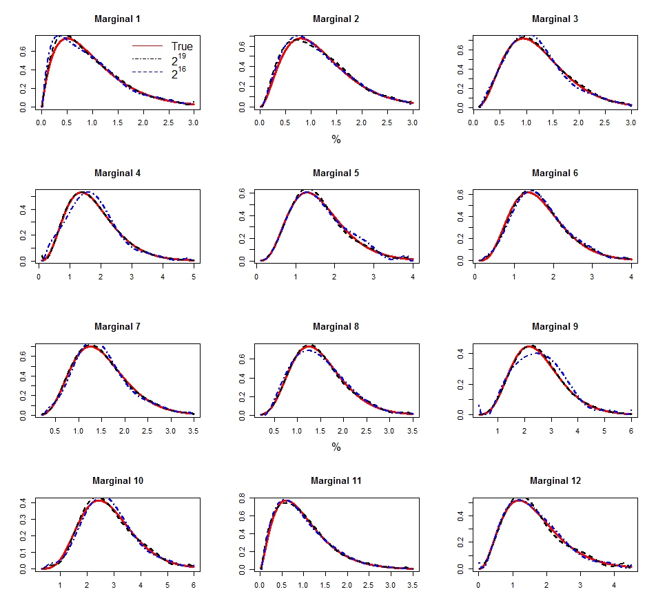
To illustrate the real computational benefit of using low discrepancy sequences, we consider two distributions of dimensions $10$ and $12$ respectively. These distributions have been generated as products of independent Gamma distributions with different parameters. A $5$-point grid will require $5^{10}=9,765,625$ points in $10$ dimensions and $244,140,625$ points in $12$ dimensions and will likely still yield inaccurate estimates, as illustrated by an inability of $n-$point grids to capture various shapes when $n$ is small in Figures 4 and 5.

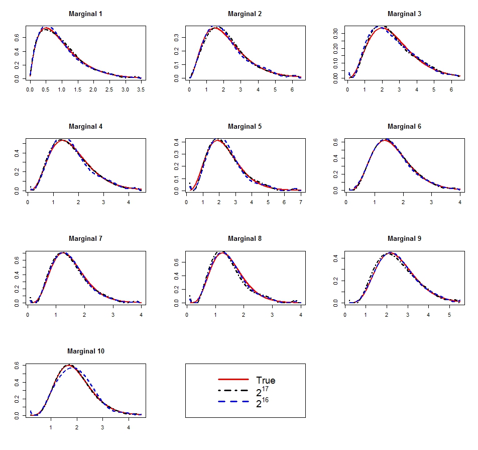
Figure 6 shows that for $s=10$, very accurate estimates can be obtained using LDS with as little as $2^{16}$ points ($150$ times fewer than a $5$-point grid). Although estimates obtained using $2^{17}$ points are even more accurate, the difference between the two is very small suggesting that our estimates have started to converge to the true marginals. For $12$-dimensional Gamma, $2^{16}$ points give reasonably accurate estimates and the convergence is achieved by $2^{19}(=524,288)$ points as can be seen in Figure 7. However, this is negligible compared to the $244$ million points required for a $5$-point grid.

References

- [1] Cheney, W. and Kincaid, D. (2004). Numerical Mathematics and Computing (5th ed.). Thomson.
- [2] Kress, R. (1998). Numerical Analysis. Springer.
- [3] L’Ecuyer, P.L. and Munger, D. (2016). Algorithm 958: Lattice Builder: A general software tool for constructing rank-1 lattice rules. ACM Transactions on Mathematical Software, 42, Article 15.
- [4] Leobacher, G. Pillichshammer, F. (2014). Introduction to Quasi-Monte Carlo Integration and Applications. Birkhauser.
- [5] Dick, J. and Pillichshammer, F. (2010). Digital nets and Sequences. Cambridge.
- [6] Lemieux, C. (2009). Monte Carlo and Quasi-Monte Carlo Sampling. Springer.
- [7] Niederreiter, H. (1992). Random number generation and Quasi-Monte Carlo methods SIAM CBMS-NSF Regional conference series in Applied Mathematics, 63.
- [8] Sauer, T. (2012). Numerical Analysis (2nd ed.). Pearson.
- [9] Sloan, I.H. and Joe, S. (1994). Lattice methods for multiple integration. Oxford.
- [10] Rue, H. and Martino, S. and Chopin, N. (2009). Approximate Bayesian inference for latent Gaussian models by using a integrated nested Laplace approximations. Journal of Royal Statistical Society- Series B, 71, 2, 319–392.
- [11] Martin, T. and Simpson, D. and Lindgren, F. and Rue, H. (2013). Bayesian computing with INLA: New features. Computational Statistics & Data Analysis, 67, 68 – 83.
- [12] Gentle, J.E. (2007). Matrix Algebra: Theory, Computations and Applications in Statistics. Springer.