跳到论文正文
W Papers独立论文阅读器 arXiv:1911.02899 论文正文 计算阅读时间 · 0%
引用这篇论文根据当前论文元数据生成,正式投稿前建议核对。


License: arXiv.org perpetual non-exclusive license
arXiv:1911.02899v2 [eess.SY] 20 Oct 2020

A robust adaptive model predictive control framework for nonlinear uncertain systemsPubID: pubid: ©2020 John Wiley & Sons, Ltd. All rights reserved.

Johannes Köhler Affiliation: Johannes Köhler, Raffaele Soloperto, and Frank Allgöwer are with the Institute for Systems Theory and Automatic Control, University of Stuttgart, 70550 Stuttgart, Germany. (email:{\{johannes.koehler, raffaele.soloperto, frank.allgower}@ist.uni-stuttgart.de)    Peter Kötting Affiliation: Peter Kötting and Matthias A. Müller are with the Institute of Automatic Control, Leibniz University Hannover, 30167 Hannover, Germany (e-mail:koetting@stud.uni-hannover.de,mueller@irt.uni-hannover.de)    Raffaele Soloperto Affiliation: Johannes Köhler, Raffaele Soloperto, and Frank Allgöwer are with the Institute for Systems Theory and Automatic Control, University of Stuttgart, 70550 Stuttgart, Germany. (email:{\{johannes.koehler, raffaele.soloperto, frank.allgower}@ist.uni-stuttgart.de)    Frank Allgöwer Affiliation: Johannes Köhler, Raffaele Soloperto, and Frank Allgöwer are with the Institute for Systems Theory and Automatic Control, University of Stuttgart, 70550 Stuttgart, Germany. (email:{\{johannes.koehler, raffaele.soloperto, frank.allgower}@ist.uni-stuttgart.de)    Matthias A. Müller Thanks: This work was supported by the German Research Foundation under Grants GRK 2198/1 - 277536708, AL 316/12-2, and MU 3929/1-2 - 279734922. The authors thank the International Max Planck Research School for Intelligent Systems (IMPRS-IS) for supporting Raffaele Soloperto. Affiliation: Peter Kötting and Matthias A. Müller are with the Institute of Automatic Control, Leibniz University Hannover, 30167 Hannover, Germany (e-mail:koetting@stud.uni-hannover.de,mueller@irt.uni-hannover.de)
Abstract

In this paper, we present a tube-based framework for robust adaptive model predictive control (RAMPC) for nonlinear systems subject to parametric uncertainty and additive disturbances. Set-membership estimation is used to provide accurate bounds on the parametric uncertainty, which are employed for the construction of the tube in a robust MPC scheme. The resulting RAMPC framework ensures robust recursive feasibility and robust constraint satisfaction, while allowing for less conservative operation compared to robust MPC schemes without model/parameter adaptation. Furthermore, by using an additional mean-squared point estimate in the objective function the framework ensures finite-gain ℒ2\mathcal{L}_{2} stability w.r.t. additive disturbances.

As a first contribution we derive suitable monotonicity and non-increasing properties on general parameter estimation algorithms and tube/set based RAMPC schemes that ensure robust recursive feasibility and robust constraint satisfaction under recursive model updates. Then, as the main contribution of this paper, we provide similar conditions for a tube based formulation that is parametrized using an incremental Lyapunov function, a scalar contraction rate and a function bounding the uncertainty. With this result, we can provide simple constructive designs for different RAMPC schemes with varying computational complexity and conservatism. As a corollary, we can demonstrate that state of the art formulations for nonlinear RAMPC are a special case of the proposed framework. We provide a numerical example that demonstrates the flexibility of the proposed framework and showcase improvements compared to state of the art approaches.

Index Terms: 
Nonlinear MPC, Constrained control, Adaptive control, Uncertain systems.

I Introduction

Model predictive control (MPC) [1] is an optimization based control strategy that can cope with complex nonlinear systems and general nonlinear constraints on state and input. The performance and theoretical properties of MPC schemes can be highly dependent on accurate prediction models. In particular, neglecting possible computational limitations, the lack of an accurate prediction model is one of the main practical challenges for MPC implementations. This has motivated an increasing amount of research focused on online model adaptation/learning in MPC, spanning the last two decades [2, 3, 4], with current research focused on robust adaptive formulations [5, 6, 7, 8, 9, 10, 11, 12], dual/learning formulations [13, 14] and machine learning based approaches [15, 16, 17, 18]. However, all of these approaches suffer from at least one of the following shortcomings:

  1. a)

    limitation to restrictive system classes, such as linear systems [5, 6, 7, 8] or feedback linearizable systems [9],

  2. b)

    failure to provide theoretical guarantees regarding recursive feasibility, closed-loop stability and constraint satisfaction [14, 15, 16, 18],

  3. c)

    significant increase in the computational complexity [11, Chap. 10.4], [14, 15, 17],

  4. d)

    overly conservative formulation [10], [11, Chap. 10.5], [12, 17].

In this paper we provide a novel framework for RAMPC that addresses all these challenges for a class of nonlinear uncertain systems.

Related work

In general, RAMPC schemes [5, 6, 7, 8, 9, 10, 11, 12] use set membership estimation to provide a set of non falsified parameters, which is utilized in a robust tube-based MPC approach to provide robustness w.r.t. uncertain parameters and disturbances. One of the main differentiating factors among the above mentioned approaches is the parametrization of the parameter set and the construction of the robust tube that confines all uncertain predicted trajectories. These design choices highly effect the computational complexity and conservatism of the resulting scheme. In general, guaranteeing robust recursive feasibility under online adapted models is highly dependent on the interplay of the considered parametrizations and, hence, results to be non trivial in the case of nonlinear uncertain systems.

Approaches for general linear uncertain systems with polytopic tubes can be found in [6, 7, 8]. The special case of finite impulse response (FIR) systems and unknown constant/time-varying offsets are discussed in [5] and [19], respectively.

One key challenge in the design of RAMPC schemes for nonlinear systems is the requirement of a suitable robust MPC approach that is applicable to nonlinear systems with parametric uncertainty, which is currently an active research field [20, 21, 22, 23]. Recently, in [9] a RAMPC scheme for the special case of feedback linearizable nonlinear systems has been proposed using boundary layer control [20]. Except for this recent approach for feedback linearizable systems, existing RAMPC schemes for nonlinear systems with theoretical guarantees have been developed exclusively11 1 In [24] the approach in [10] has been extended to time-varying parameters, but only a min-max RAMPC formulation was considered, which is not computationally tractable. by Martin Guay and coauthors [10, 11, 12, 25, 26].

In particular, parameter update schemes have been developed that provide guaranteed bounds on the parameter error for a large class of nonlinear systems, including continuous time [10], discrete time [12], time varying [25], and nonlinearly parametrized systems [26], compare [11] for a general overview. However, all these approaches consider a simple robust tube approach based on Lipschitz constants similar to [27, 28], which can be prohibitively conservative in many scenarios, see numerical comparisons in [23, 29, 30].

On the other hand, in the last decade several robust MPC approaches for nonlinear systems have been developed, using: interval arithmetic [31]; boundary layer control for feedback linearizable systems [20]; min\min–max\max differential inequalities [21]; control contraction metrics [22]; and incremental Lyapunov functions [23, 32]. Employing more recent robust MPC approaches may alleviate some of the inherent limitations of state of the art RAMPC schemes. However, due to difficulties in the analysis, these robust MPC approaches have not yet been employed to design suitable nonlinear RAMPC schemes. As stated in22 2 A possible exception to this statement may be the RAMPC scheme in the thesis [9], that addresses similar challenges as the proposed approach, but is limited to continuous time feedback linearizable systems.  [9]: A tractable nonlinear AMPC approach that does not rely on unrealistic assumptions has yet to be developed.

More recently, machine learning inspired and data driven approaches for model identification/adaptation/refinement have gained a lot of attention, e.g. using Gaussian Processes (GPs) [15, 16], (local) weighted Bayesian linear regression (wBLR) [18] and kinky inference [17], to name a few. Such approaches use different (potentially less restrictive) a priori assumptions [15, 16, 17] and also perform well in some experiments [15, 16, 18]. However, currently the corresponding robust MPC literature that can provide theoretical guarantees using such models seems rather immature compared to classical RAMPC approaches, see [33] for a more general discussion.

Contribution

In this paper, we present a tube-based framework for robust adaptive model predictive control (RAMPC) for a class of uncertain nonlinear systems subject to additive disturbances and parametric uncertainty. The paper contains the following contributions: (i) present a general theoretical framework for nonlinear RAMPC; (ii) provide a computationally efficient RAMPC framework by extending the robust MPC framework in [23] to allow for recursive model updates; (iii) provide explicit design procedures, which contain the approaches in  [10, 11, 12] as a special case.

First, given the plethora and diversity of existing robust MPC formulations for nonlinear systems [20, 21, 22, 23, 27, 28, 29, 31, 32] and parameter set updates [5, 6, 7, 8, 9, 11, 25, 26], we consider the general problem of providing conditions on the robust MPC tube propagation and set updates. In particular, we provide general conditions regarding overapproximation of the uncertainty, nonincreasingness of the parameter set, and monotonicity properties of the tube propagation, that ensure robust recursive feasibility and robust constraint satisfaction.

Second, as the main contribution of this paper, we provide a framework for computationally efficient nonlinear RAMPC based on the nonlinear robust MPC approach in [23]. We consider nonlinear systems linear in uncertain parameters subject to bounded additive disturbances with nonlinear Lipschitz continuous constraints. We assume that the nominal nonlinear system is exponentially incrementally stabilizable with some known contraction rate ρ\rho and incremental Lyapunov function VδV_{\delta}. Furthermore, we design a nonlinear (state and input dependent) function w~\tilde{w} that bounds the difference between the nominal and uncertain system. The tube dynamic is then defined by a scalar ss that depends on the contraction rate ρ\rho and the function w~\tilde{w}. This formulation allows us to compute an efficient constraint tightening, while only moderately increasing the computational demand with respect to a nominal MPC scheme. As the main technical contribution, given this parametrization using ρ,w~,Vδ\rho,\tilde{w},V_{\delta}, we derive suitable conditions that ensure robust recursive feasibility and robust constraint satisfaction. Thus we extend the robust MPC framework in [23] to allow for online parameter updates and reduction in the conservatism. Furthermore, we show that by designing the objective function based on an additional mean squared point estimate θ^\hat{\theta}, we can guarantee finite gain ℒ2\mathcal{L}_{2} stability w.r.t. disturbances, extending the stability results in [6, 8] to nonlinear systems.

Next, given the general conditions for this RAMPC framework, we provide explicit design procedures that satisfy the posed conditions. In particular, we propose a moving window parameter set update yielding online shrinking finite complexity hypercubes that contain the true parameters. Then, we provide two simple designs regarding the function w~\tilde{w} that ensure robustness, while allowing for a flexible trade off regarding conservatism and computational complexity. Furthermore, we demonstrate that by using a ball as an ”incremental Lyapunov function” VδV_{\delta}, we recover the approach in [10, 11, 12] as a special case.

Finally, we demonstrate the applicability and advantages of the proposed framework with a nonlinear example.

To summarize, the resulting nonlinear RAMPC framework: (i) reduces conservatism online using set membership updates, (ii) improves performance using a mean squared cost, (iii) can be significantly less conservative compared to state of the art approaches, i.e. [10, 11, 12], (iv) provides a flexible trade off regarding conservativism and computational complexity, and (v) avoids computationally expensive online optimizations stemming from matrix variables [15, 21], piece-wise definitions [17], scenario trees [14], or general min\min–max\max optimization [11, Chap. 10.4].

The paper is structured as follows: Section II discusses the general problem of RAMPC. Section III presents the general theory regarding the proposed framework for nonlinear RAMPC with a corresponding design procedure. Section IV provides a numerical example to demonstrate the applicability and advantages of the proposed approach. Section V concludes the paper. In Appendix -A, an alternative design for the terminal ingredients is presented.

Notation

The quadratic norm with respect to a positive definite matrix Q=Q⊤Q=Q^{\top} is denoted by ‖x‖Q2=x⊤​Q​x\|x\|_{Q}^{2}=x^{\top}Qx and the minimal and maximal eigenvalue of QQ are denoted by λmin​(Q)\lambda_{\min}(Q) and λmax​(Q)\lambda_{\max}(Q), respectively. The positive real numbers are ℝ≥0={r∈ℝ|r≥0}\mathbb{R}_{\geq 0}=\{r\in\mathbb{R}|r\geq 0\}. The vertices of a polytopic set Θ\Theta are denoted by θi∈Vert​(Θ)\theta^{i}\in\text{Vert}(\Theta). By 𝒦∞\mathcal{K}_{\infty} we denote the class of functions α:ℝ≥0→ℝ≥0\alpha:\mathbb{R}_{\geq 0}\rightarrow\mathbb{R}_{\geq 0}, which are continuous, strictly increasing, unbounded and satisfy α⁡(0)=0\alpha(0)=0. Denote the unit hypercube by 𝔹∞:={θ|‖θ‖∞≤1}\mathbb{B}_{\infty}:=\{\theta|~\|\theta\|_{\infty}\leq 1\} and the unit ball by 𝔹2:={θ|‖θ‖≤1}\mathbb{B}_{2}:=\{\theta|~\|\theta\|\leq 1\}. The Minkowski sum and Pontryagin difference for two sets 𝔸,𝔹⊆ℝn\mathbb{A},\mathbb{B}\subseteq\mathbb{R}^{n} are denoted by 𝔸⊕𝔹:={a+b|a∈𝔸,b∈𝔹}\mathbb{A}\oplus\mathbb{B}:=\{a+b|~a\in\mathbb{A},b\in\mathbb{B}\} and 𝔸⊖𝔹:={c|c+b∈𝔸​∀b∈𝔹}\mathbb{A}\ominus\mathbb{B}:=\{c|~c+b\in\mathbb{A}\forall b\in\mathbb{B}\}, respectively.

II Setup and general theory

In this section, we derive the general conditions for tube-based RAMPC in terms of set predictions, before presenting the proposed RAMPC framework in Section III. We consider a nonlinear discrete time system of the form

xt+1=fw​(xt,ut,dt,θ∗),\displaystyle x_{t+1}=f_{w}(x_{t},u_{t},d_{t},\theta^{*}), (1)

with state xt∈ℝnx_{t}\in\mathbb{R}^{n}, control input u∈ℝmu\in\mathbb{R}^{m}, disturbances dt∈𝔻⊂ℝqd_{t}\in\mathbb{D}\subset\mathbb{R}^{q}, time t∈ℕt\in\mathbb{N}, and perturbed dynamics fwf_{w} with some unknown but constant parameters θ∗∈ℝp\theta^{*}\in\mathbb{R}^{p}. We consider point-wise in time state and input constraints

(xt,ut)∈𝒵,t≥0,\displaystyle(x_{t},u_{t})\in\mathcal{Z},\quad t\geq 0, (2)

with some compact nonlinear constraint set

𝒵={(x,u)∈ℝn+m|hj(x,u)≤0,j=1,…,r}.\displaystyle\mathcal{Z}=\{(x,u)\in\mathbb{R}^{n+m}|~h_{j}(x,u)\leq 0,~j=1,\dots,r\}. (3)

Denote by 𝒵x\mathcal{Z}_{x} the projection of 𝒵\mathcal{Z} on ℝn\mathbb{R}^{n}. The following assumption characterizes the uncertainty in the parameters θ\theta.

Assumption 1.

At each time step t∈ℕt\in\mathbb{N}, a parameter set Θt\Theta_{t} is computed satisfying Θt+1⊆Θt⊆Θ0\Theta_{t+1}\subseteq\Theta_{t}\subseteq\Theta_{0} and θ∗∈Θt\theta^{*}\in\Theta_{t}.

For simplicity, the following presentation does not consider any stabilizing feedback κ\kappa, which is typically used in robust tube MPC, since it complicates the exposition. The following results can, however, easily be adapted to this case. We consider some map Φ\Phi to predict sets 𝕏k|t\mathbb{X}_{k|t}, that characterizes the tube.

Assumption 2.

There exists a map Φ:2ℝn×ℝm×2ℝq→2ℝn\Phi:2^{\mathbb{R}^{n}}\times\mathbb{R}^{m}\times 2^{\mathbb{R}^{q}}\rightarrow 2^{\mathbb{R}^{n}}, such that for any (𝕏,u)⊆𝒵(\mathbb{X},u)\subseteq\mathcal{Z}, Θ⊆Θ0\Theta\subseteq\Theta_{0}, we have

fw​(x,u,d,θ)∈Φ⁡(𝕏,u,Θ),\displaystyle f_{w}(x,u,d,\theta)\in\Phi(\mathbb{X},u,\Theta), (4)

for any x∈𝕏x\in\mathbb{X}, d∈𝔻d\in\mathbb{D} and θ∈Θ\theta\in\Theta. Furthermore, the function Φ\Phi satisfies the following monotonicity property

Φ⁡(𝕏′,u,Θ′)⊆Φ⁡(𝕏,u,Θ),\displaystyle\Phi(\mathbb{X}^{\prime},u,\Theta^{\prime})\subseteq\Phi(\mathbb{X},u,\Theta), (5)

for any (𝕏′,u)⊆(𝕏,u)⊆𝒵(\mathbb{X}^{\prime},u)\subseteq(\mathbb{X},u)\subseteq\mathcal{Z}, and any Θ′⊆Θ⊆Θ0\Theta^{\prime}\subseteq\Theta\subseteq\Theta_{0}.

Given these conditions, a general tube based robust adaptive MPC scheme can be formulated with the following optimization problem using the measured state xtx_{t}, the parameter set Θt\Theta_{t} and some cost function JNJ_{N}:

minu⋅|t,𝕏⋅|t⁡JN​(𝕏⋅|t,u⋅|t)\displaystyle\min_{u_{\cdot|t},\mathbb{X}_{\cdot|t}}J_{N}(\mathbb{X}_{\cdot|t},u_{\cdot|t}) (6a)
s.t. xt∈𝕏0|t,\displaystyle x_{t}\in\mathbb{X}_{0|t}, (6b)
𝕏k+1|t⊇Φ⁡(𝕏k|t,uk|t,Θt),\displaystyle\mathbb{X}_{k+1|t}\supseteq\Phi(\mathbb{X}_{k|t},u_{k|t},\Theta_{t}), (6c)
(𝕏k|t,uk|t)⊆𝒵,\displaystyle(\mathbb{X}_{k|t},u_{k|t})\subseteq\mathcal{Z}, (6d)
k=0,…,N−1,\displaystyle k=0,\dots,N-1, (6e)
Φ⁡(𝕏N|t,uN|t,Θt)⊆𝕏N|t,(𝕏N|t,uN|t)⊆𝒵.\displaystyle\Phi(\mathbb{X}_{N|t},u_{N|t},\Theta_{t})\subseteq\mathbb{X}_{N|t},~(\mathbb{X}_{N|t},u_{N|t})\subseteq\mathcal{Z}. (6f)

The minimizers are denoted by u⋅|t∗u_{\cdot|t}^{*}, 𝕏⋅|t∗\mathbb{X}_{\cdot|t}^{*}. The corresponding closed loop input is given by ut=u0|t∗u_{t}=u_{0|t}^{*}.

The following theorem shows that this general set approach directly ensures robust recursive feasibility and robust constraint satisfaction.

Theorem 1.

Let Assumptions 1 and 2 hold and suppose that Problem (6) is feasible at t=0t=0. Then Problem (6) is feasible for all t∈ℕt\in\mathbb{N} and the constraints (2) are satisfied for the resulting closed loop system.

Proof.

The proof is similar to standard results in robust MPC, extended to the adaptive setting using a suitable monotonicity property in Assumption 2, compare e.g. [34] for similar arguments. In particular, consider any set 𝕏0|t+1\mathbb{X}_{0|t+1} satisfying 𝕏1|t∗⊇𝕏0|t+1∋xt+1\mathbb{X}^{*}_{1|t}\supseteq\mathbb{X}_{0|t+1}\ni x_{t+1}, for example 𝕏0|t+1=𝕏1|t∗\mathbb{X}_{0|t+1}=\mathbb{X}^{*}_{1|t}, which satisfies xt+1∈𝕏0|t+1x_{t+1}\in\mathbb{X}_{0|t+1} due to the overapproximation property (4). Then the candidate solution uk|t+1=uk+1|t∗u_{k|t+1}=u^{*}_{k+1|t}, uN|t+1=uN|t∗u_{N|t+1}=u^{*}_{N|t}, is a feasible solution with33 3 In approaches directly utilizing sets, e.g. [6, 7, 32], the candidate solution 𝕏k|t+1=𝕏k+1|t∗\mathbb{X}_{k|t+1}=\mathbb{X}^{*}_{k+1|t} is standard. However, most tube-based approaches, e.g. [8, 12, 23, 27, 28, 31], including the proposed approach, consider a candidate solution that does not necessarily satisfy 𝕏k|t+1=𝕏k+1|t∗\mathbb{X}_{k|t+1}=\mathbb{X}^{*}_{k+1|t}, but 𝕏k|t+1⊆𝕏k+1|t∗\mathbb{X}_{k|t+1}\subseteq\mathbb{X}^{*}_{k+1|t}. 𝕏k|t+1=𝕏k+1|t∗\mathbb{X}_{k|t+1}=\mathbb{X}^{*}_{k+1|t}, 𝕏N|t+1=𝕏N−1|t+1=𝕏N|t∗\mathbb{X}_{N|t+1}=\mathbb{X}_{N-1|t+1}=\mathbb{X}^{*}_{N|t}, due to the monotonicity of the operator Φ\Phi (5), the non-expansiveness of the parameter set Θt\Theta_{t} (Ass. 1) and the terminal constraint (6f). ∎

The presented formulation in (6) and the corresponding theoretical properties in Theorem 1 are quite intuitive. However, without any tractable formulation for the sets 𝕏\mathbb{X}, Θ\Theta and the propagation Φ\Phi this formulation cannot be used in practice. In this sense, the general formulation (6) and Theorem 1 are similar to the min\min–max\max formulation in [11, Chap. 10.4], as they provide general theoretical results but are not directly amenable to practical implementation.

Existing tube formulations

In the following, we briefly elaborate on different parametrizations for 𝕏\mathbb{X} and Θ\Theta which have been considered in the robust and robust adaptive MPC literature.

For linear systems, typically polytopic sets Θ\Theta are considered and the tube is parametrized by a polytope 𝕏t={x|H​x≤αt}\mathbb{X}_{t}=\{x|~Hx\leq\alpha_{t}\} with HH fixed offline. The inclusion (6c) can then be implemented using linear inequality constraints, compare e.g. [6, 7, 8] and [35, Chap. 5]. In particular, the approach in [6] considers general polytopic parameter sets Θ\Theta and a homothetic tube approach, which directly formulates (6c) as equivalent linear inequality constraints, using additional dual variables Λ\Lambda. In [7], zonotope parameter sets Θt={Πθθ≤πt}\Theta_{t}=\{\Pi_{\theta}\theta\leq\pi_{t}\} with Πθ\Pi_{\theta} fixed, are considered and the set inclusion (6c) is implemented using α\alpha as optimization variables. In [8], only scalars s,ηs,\eta are used in parametrizing a hypercube parameter set Θt=θ¯t⊕ηt​𝔹∞\Theta_{t}=\overline{\theta}_{t}\oplus\eta_{t}\mathbb{B}_{\infty} and the polytopic tube 𝕏t=x¯t⊕st⋅𝒫\mathbb{X}_{t}=\overline{x}_{t}\oplus s_{t}\cdot\mathcal{P}. A more detailed comparison regarding computational complexity and conservatism of these linear RAMPC approaches can be found in [8].

In the papers [10, 11, 12] by Martin Guay and coauthors, the parameter set Θ\Theta and the tube 𝕏\mathbb{X} are given by a scaled ball, i.e., Θt=θ¯t⊕ηt​𝔹2\Theta_{t}=\overline{\theta}_{t}\oplus\eta_{t}\mathbb{B}_{2} and 𝕏t=x¯t⊕st​𝔹2\mathbb{X}_{t}=\overline{x}_{t}\oplus s_{t}\mathbb{B}_{2}. This simple scalar parametrization is crucial in providing a tractable formulation, which allows the implementation of the set inclusion (6c) using scalar nonlinear dynamics for ss. However, this can also yield very conservative bounds on the tube size ss along the prediction horizon, compare the numerical example in Section IV.

In [9], a hyper box Θ\Theta and a box shaped tube 𝕏\mathbb{X} are considered resulting from a boundary layer controller, while the boundary layer thickness ss is predicted using nonlinear dynamics for ss, compare [20].

Regarding general robust MPC schemes for nonlinear systems (without parameter adaptation and often without parametric uncertainty): In [31] an interval arithmetic approach is considered, which improves Lipschitz based approaches [27, 28] by using a more flexible hyperbox tube 𝕏\mathbb{X}. However, similar to the Lipschitz based approach, unless the considered tube parametrization 𝕏\mathbb{X} contains a robust positive invariant (RPI) set, the tube is growing unbounded along the prediction horizon and thus only short horizons and/or small uncertainty can be considered. In [22, 32] additive disturbances are considered and a fixed RPI set 𝕏\mathbb{X} is computed offline as an incremental Lyapunov function or using control contraction metrics.

In [21], the tube is parametrized with online optimized matrices Pt∈ℝn×nP_{t}\in\mathbb{R}^{n\times n}, i.e., 𝕏t={x|‖x¯t−x‖Pt2≤1}\mathbb{X}_{t}=\{x|~\|\overline{x}_{t}-x\|_{P_{t}}^{2}\leq 1\}, where (6c) is ensured using min\min–max\max differential inequalities.

In [23], a scalar ss is used to parametrize the tube 𝕏\mathbb{X} with a given incremental Lyapunov function VδV_{\delta}, i.e., 𝕏t={x|Vδ​(x,x¯t)≤st}\mathbb{X}_{t}=\{x|~V_{\delta}(x,\overline{x}_{t})\leq s_{t}\}, while the tube propagation (6c) is formulated as nonlinear dynamics for ss, similar to [20, 28]. Thus, this approach shares the simple scalar characterization of the tube used in [10, 11, 12]. In the next section, we concretize the rather abstract conditions and assumptions for the specific parametrization of 𝕏\mathbb{X} and Φ\Phi based on the robust MPC approach in [23].

III Proposed framework - theoretical analysis

The results in this section are the main contribution of this paper. In the following, we derive the proposed framework for nonlinear RAMPC using the nonlinear robust MPC framework in [23]. In Section III-A the general conditions and assumptions are introduced. The RAMPC optimization problem is presented in Section III-B. Constraint satisfaction and robust recursive feasibility are established in Theorem 2 in Section III-C. Theorem 3 in Section III-D shows finite gain ℒ2\mathcal{L}_{2} stability using a least mean square (LMS) point estimate and a suitable stage cost ℓ:𝒵→ℝ\ell:\mathcal{Z}\rightarrow\mathbb{R}. Section III-E provides explicit design procedures and the overall algorithm. In Section III-F we demonstrate that state of the art approaches [10, 11, 12] are contained as a special case of the proposed formulation. Section III-G discusses some extensions and open issues.

III-A Assumptions

In the following, we introduce assumptions regarding the nonlinear system fwf_{w}, including model structure (Ass. 3), nominal parameter updates (Ass. 4) , stabilizability (Ass. 5), designed functions w~\tilde{w} (Ass. 6) and terminal ingredients (Ass. 7).

The following standing assumption characterizes the considered class of nonlinear systems.

Assumption 3.

There exist (locally) Lipschitz continuous functions gi:𝒵→ℝng_{i}:\mathcal{Z}\rightarrow\mathbb{R}^{n}, i=1,…,pi=1,\dots,p and a matrix E∈ℝn×qE\in\mathbb{R}^{n\times q}, such that the nonlinear system (1) is given by

fw​(x,u,d,θ)=\displaystyle f_{w}(x,u,d,\theta)= f⁡(x,u)+G⁡(x,u)​θ+E​d,\displaystyle f(x,u)+G(x,u)\theta+Ed, (7)
G⁡(x,u):=\displaystyle G(x,u):= [g1​(x,u),…,gp​(x,u)].\displaystyle[g_{1}(x,u),\dots,g_{p}(x,u)].

There exists a known set 𝔻⊂ℝq\mathbb{D}\subset\mathbb{R}^{q} with 0∈𝔻0\in\mathbb{D}, such that the additive disturbance satisfy dt∈𝔻d_{t}\in\mathbb{D} for all t≥0t\geq 0.
The functions hjh_{j} in (3) are (locally) Lipschitz continuous.

The main restriction in the posed conditions is that the parameters θ\theta enter affinely and the disturbances are only additive. Except for the paper [26] which explicitly handles the intricate case of nonlinearly parametrized systems, most existing RAMPC schemes for linear [5, 6, 7, 8, 19] and nonlinear systems [9, 10, 11, 12, 25] also consider a linear parametrization in θ\theta and additive disturbances dtd_{t}. In Section III-G we discuss how to relax the Lipschitz continuity of hjh_{j} and extend the proposed approach to time varying parameters θt∗\theta_{t}^{*}.

In the following, we consider a nominal prediction model fθ¯t​(x,u):=f⁡(x,u)+G⁡(x,u)​θ¯tf_{\overline{\theta}_{t}}(x,u):=f(x,u)+G(x,u)\overline{\theta}_{t} with online determined parameters θ¯t\overline{\theta}_{t} satisfying the following assumption.

Assumption 4.

At each time tt, we compute a point estimate θ¯t\overline{\theta}_{t} with a corresponding uncertainty set Θ~t\widetilde{\Theta}_{t} that satisfy

θ∗∈θ¯t+1⊕Θ~t+1⊆θ¯t⊕Θ~t,∀t≥0.\displaystyle\theta^{*}\in\overline{\theta}_{t+1}\oplus\widetilde{\Theta}_{t+1}\subseteq\overline{\theta}_{t}\oplus\widetilde{\Theta}_{t},~\forall t\geq 0. (8)

with some initial known prior parameter set θ¯0⊕Θ~0\overline{\theta}_{0}\oplus\widetilde{\Theta}_{0}.

In essence, this assumption is equivalent to Assumption 1, formulated in terms of a nominal point θ¯\overline{\theta} and an uncertain set Θ~\widetilde{\Theta}. Correspondingly, the change in parameters satisfies Δ​θ¯t:=θ¯t+1−θ¯t∈Δ​Θ~t:=Θ~t⊖Θ~t+1\Delta\overline{\theta}_{t}:=\overline{\theta}_{t+1}-\overline{\theta}_{t}\in\Delta\widetilde{\Theta}_{t}:=\widetilde{\Theta}_{t}\ominus\widetilde{\Theta}_{t+1}. Set membership updates for Θ~t,θ¯t\widetilde{\Theta}_{t},\overline{\theta}_{t} satisfying Assumption 4 will be introduced in Sec. III-E, Alg. 1. The prediction mismatch satisfies

xt+1−fθ¯t​(xt,ut)∈𝕎Θ~t,𝔻​(xt,ut),\displaystyle x_{t+1}-f_{\overline{\theta}_{t}}(x_{t},u_{t})\in\mathbb{W}_{\widetilde{\Theta}_{t},\mathbb{D}}(x_{t},u_{t}), (9)
𝕎Θ~,𝔻(x,u):={dw∈ℝn|dw=d+G(x,u)θ~,d∈𝔻,θ~∈Θ~}.\displaystyle\mathbb{W}_{\widetilde{\Theta},\mathbb{D}}(x,u):=\{d_{w}\in\mathbb{R}^{n}|~d_{w}=d+G(x,u)\tilde{\theta},~d\in\mathbb{D},~\tilde{\theta}\in\widetilde{\Theta}\}.

In order to design a suitable tube 𝕏\mathbb{X}, we assume that the system is locally incrementally stabilizable, similar to [23, Ass. 2].

Assumption 5.

There exists a continuous incremental Lyapunov function Vδ:ℝn×ℝn→ℝ≥0V_{\delta}:\mathbb{R}^{n}\times\mathbb{R}^{n}\rightarrow\mathbb{R}_{\geq 0} satisfying

cδ,l​‖x−z‖≤Vδ​(x,z)≤\displaystyle c_{\delta,l}\|x-z\|\leq V_{\delta}(x,z)\leq cδ,u​‖x−z‖,\displaystyle c_{\delta,u}\|x-z\|, (10a)
for all x,z∈ℝnx,z\in\mathbb{R}^{n} with constants cδ,lc_{\delta,l}, cδ,u>0c_{\delta,u}>0. Furthermore, there exist a control law κ:𝒵x×𝒵→ℝm\kappa:\mathcal{Z}_{x}\times\mathcal{Z}\rightarrow\mathbb{R}^{m}, and constants δl​o​c\delta_{loc}, κmax>0\kappa_{\max}>0, such that the following properties hold for all (z,v)∈𝒵(z,v)\in\mathcal{Z}, (x,κ⁡(x,z,v))∈𝒵(x,\kappa(x,z,v))\in\mathcal{Z}, Vδ​(x,z)≤δl​o​cV_{\delta}(x,z)\leq\delta_{loc}, and all θ¯∈θ¯0⊕Θ~0\overline{\theta}\in\overline{\theta}_{0}\oplus\widetilde{\Theta}_{0}:
‖κ⁡(x,z,v)−v‖≤\displaystyle\|\kappa(x,z,v)-v\|\leq κmax​Vδ​(x,z),\displaystyle\kappa_{\max}V_{\delta}(x,z), (10b)
Vδ​(x+,z+)≤\displaystyle V_{\delta}(x^{+},z^{+})\leq ρθ¯​Vδ​(x,z),\displaystyle\rho_{\overline{\theta}}V_{\delta}(x,z), (10c)
with x+=fθ¯​(x,κ⁡(x,z,v))x^{+}=f_{\overline{\theta}}(x,\kappa(x,z,v)), z+=fθ¯​(z,v)z^{+}=f_{\overline{\theta}}(z,v) and some ρθ¯>0\rho_{\overline{\theta}}>0. Furthermore, the following norm-like condition holds for any x1,x2,Δ​x∈ℝnx_{1},x_{2},\Delta x\in\mathbb{R}^{n}:
Vδ​(x1+Δ​x,x2)≤Vδ​(x1,x2)+Vδ​(x2+Δ​x,x2).\displaystyle V_{\delta}(x_{1}+\Delta x,x_{2})\leq V_{\delta}(x_{1},x_{2})+V_{\delta}(x_{2}+\Delta x,x_{2}). (10d)
In addition, there exists a constant Lδ≥0L_{\delta}\geq 0, such that the following continuity bound holds for any x1,x2,Δ​x∈ℝnx_{1},x_{2},\Delta x\in\mathbb{R}^{n}:
Vδ​(x1,x2+Δ​x)≤(1+Lδ​‖Δ​x‖)​Vδ​(x1−Δ​x,x2).\displaystyle V_{\delta}(x_{1},x_{2}+\Delta x)\leq(1+L_{\delta}\|\Delta x\|)V_{\delta}(x_{1}-\Delta x,x_{2}). (10e)

In case ρθ¯<1\rho_{\overline{\theta}}<1, conditions (10a)–(10c) imply that VδV_{\delta} is an incremental exponential Lyapunov function with some Lipschitz continuous feedback κ\kappa. A detailed discussion how existing tube parametrizations are related to Assumption 5 can be found in [23, Remark 1]. The norm-like inequality (10d) and Lipschitz like condition (10e) are, for example, satisfied by polytopes Vδ​(x,z)=maxi⁡Pi​(x−z)V_{\delta}(x,z)=\max_{i}P_{i}(x-z), ellipsoids Vδ​(x,z)=‖x−z‖PV_{\delta}(x,z)=\|x-z\|_{P} and functions of the form44 4 A proof of inequality (10e) for P⁡(z)P(z) Lipschitz continuous can be found in [36, Prop. 15]. Examples of such incremental Lyapunov functions can be found in [34, 36, 37] using a quasi-LPV parametrization, compare [37] for a corresponding LMI design procedure. Vδ​(x,z)=‖x−z‖P⁡(z)V_{\delta}(x,z)=\|x-z\|_{P(z)}.

In the following, we denote the set Ψ:={(x,z,v)∈ℝn×𝒵|(x,κ(x,z,v))∈𝒵,Vδ(x,z)≤δl​o​c}\Psi:=\{(x,z,v)\in\mathbb{R}^{n}\times\mathcal{Z}|~(x,\kappa(x,z,v))\in\mathcal{Z},~V_{\delta}(x,z)\leq\delta_{loc}\}. For each constraint (3), we compute constants cj≥0c_{j}\geq 0, j=1,…,rj=1,\dots,r satisfying

hj​(x,κ⁡(x,z,v))−hj​(z,v)≤cj​Vδ​(x,z),\displaystyle h_{j}(x,\kappa(x,z,v))-h_{j}(z,v)\leq c_{j}V_{\delta}(x,z), (11)

for all (x,z,v)∈Ψ(x,z,v)\in\Psi, which will later be used in the design. Existence of finite constants cjc_{j} satisfying (11) follows from hjh_{j} Lipschitz continuous and the bound on Vδ,κV_{\delta},\kappa in (10a)–(10b).

The smallest contraction rate ρθ\rho_{\theta} for a given value of θ∈Θ0\theta\in\Theta_{0} satisfying (10c) is given by

ρθ:=max(x,z,v)∈Ψ⁡Vδ​(fθ​(x,κ⁡(x,z,v)),fθ​(z,v))Vδ​(x,z).\displaystyle\rho_{\theta}:=\max_{(x,z,v)\in\Psi}\dfrac{V_{\delta}(f_{\theta}(x,\kappa(x,z,v)),f_{\theta}(z,v))}{{V_{\delta}(x,z)}}. (12)

The following proposition provides a bound on the change of ρθ\rho_{\theta} under changing parameters.

Proposition 1.

Let Assumptions 3 and 5 hold. For any θ\theta, Δ​Θ\Delta\Theta there exists a Lipschitz constant Lρ,θ,Δ​Θ≥0L_{\rho,\theta,\Delta\Theta}\geq 0 according to (15), such that for any θ+∈θ⊕Δ​Θ⊆Θ0{\theta}^{+}\in{\theta}\oplus\Delta{\Theta}\subseteq\Theta_{0}, the contraction rate ρθ\rho_{\theta} satisfies

ρθ+≤ρθ+Lρ,θ,Δ​Θ.\displaystyle\rho_{{\theta}^{+}}\leq\rho_{{\theta}}+L_{\rho,\theta,\Delta{\Theta}}. (13)
Proof.

First, note that for any x1,x2,Δ​x1,Δ​x2∈ℝnx_{1},x_{2},\Delta x_{1},\Delta x_{2}\in\mathbb{R}^{n} the following continuity condition holds

Vδ​(x1+Δ​x1,x2+Δ​x2)\displaystyle V_{\delta}(x_{1}+\Delta x_{1},x_{2}+\Delta x_{2}) (14)
≤(10e)\displaystyle\stackrel{{\scriptstyle\eqref{eq:increm_e}}}{{\leq}} (1+Lδ​‖Δ​x2‖)​Vδ​(x1+Δ​x1−Δ​x2,x2)\displaystyle(1+L_{\delta}\|\Delta x_{2}\|)V_{\delta}(x_{1}+\Delta x_{1}-\Delta x_{2},x_{2})
≤(10d)\displaystyle\stackrel{{\scriptstyle\eqref{eq:increm_d}}}{{\leq}} (1+Lδ​‖Δ​x2‖)​(Vδ​(x1,x2)+Vδ​(x2+Δ​x1−Δ​x2,x2))\displaystyle(1+L_{\delta}\|\Delta x_{2}\|)(V_{\delta}(x_{1},x_{2})+V_{\delta}(x_{2}+\Delta x_{1}-\Delta x_{2},x_{2}))
≤(10a)\displaystyle\stackrel{{\scriptstyle\eqref{eq:increm_a}}}{{\leq}} (1+Lδ​‖Δ​x2‖)​(Vδ​(x1,x2)+cδ,u​‖Δ​x1−Δ​x2‖).\displaystyle(1+L_{\delta}\|\Delta x_{2}\|)(V_{\delta}(x_{1},x_{2})+c_{\delta,u}\|\Delta x_{1}-\Delta x_{2}\|).

Denote Δ​θ=θ+−θ\Delta\theta=\theta^{+}-\theta. For any (x,z,v)∈Ψ(x,z,v)\in\Psi, we have

Vδ​((fθ+​(x,κ⁡(x,z,v)),fθ+​(z,v)))\displaystyle V_{\delta}((f_{\theta^{+}}(x,\kappa(x,z,v)),f_{\theta^{+}}(z,v)))
≤(14)\displaystyle\stackrel{{\scriptstyle\eqref{eq:increm_f}}}{{\leq}} (1+Lδ​‖G⁡(z,v)​Δ​θ‖)​(Vδ​(fθ​(x,κ⁡(x,z,v)),fθ​(z,v))CLOSE\displaystyle(1+L_{\delta}\|G(z,v)\Delta\theta\|)(V_{\delta}(f_{\theta}(x,\kappa(x,z,v)),f_{\theta}(z,v))
OPEN+cδ,u​‖(G⁡(x,κ⁡(x,z,v))−G⁡(z,v))​Δ​θ‖)\displaystyle+c_{\delta,u}\|(G(x,\kappa(x,z,v))-G(z,v))\Delta\theta\|)
≤(12)\displaystyle\stackrel{{\scriptstyle\eqref{eq:rho_theta}}}{{\leq}} (1+Lδ​G¯​‖Δ​θ‖)​(ρθ+cδ,u​LG,κ​‖Δ​θ‖)​Vδ​(x,z),\displaystyle(1+L_{\delta}\overline{G}\|\Delta\theta\|)(\rho_{\theta}+c_{\delta,u}L_{G,\kappa}\|\Delta\theta\|)V_{\delta}(x,z),

where G¯=max(z,v)∈𝒵⁡‖G⁡(z,v)‖\overline{G}=\max_{(z,v)\in\mathcal{Z}}\|G(z,v)\| and LG,κL_{G,\kappa} is a suitable Lipschitz constant, given G,κG,\kappa Lipschitz and the lower bound in (10a). Thus,

Lρ,Δ​Θ:=(Lδ​G¯​ρθ+cδ,u​LG,κ)​ϵΔ​Θ+Lδ​G¯​cδ,u​LG,κ​ϵΔ​Θ2,\displaystyle L_{\rho,\Delta\Theta}:=(L_{\delta}\overline{G}\rho_{\theta}+c_{\delta,u}L_{G,\kappa})\epsilon_{\Delta\Theta}+L_{\delta}\overline{G}c_{\delta,u}L_{G,\kappa}\epsilon_{\Delta\Theta}^{2}, (15)

with ϵΔ​Θ=maxθ∈Δ​Θ⁡‖θ‖\epsilon_{\Delta\Theta}=\max_{\theta\in\Delta\Theta}\|\theta\| satisfies (13). ∎

In Sec. III-E, Prop. 3 for the special case of Vδ​(x,z)=‖x−z‖PV_{\delta}(x,z)=\|x-z\|_{P}, we will derive a simpler expression for Lρ,θ,Δ​ΘL_{\rho,\theta,\Delta\Theta}.

In order to facilitate an efficient evaluation of the uncertainty (possible model mismatch) at some point (z,v)∈𝒵(z,v)\in\mathcal{Z} or in a neighbourhood thereof, we design a function w~\tilde{w} offline, satisfying the following conditions.

Assumption 6.

Consider the functions Vδ,κV_{\delta},\kappa from Assumption 5 and the Lipschitz constant Lρ,θ¯,Δ​Θ~L_{\rho,\overline{\theta},\Delta\widetilde{\Theta}} from Prop. 1. For any sets Θ~+\widetilde{\Theta}^{+}, Δ​Θ~\Delta\widetilde{\Theta}, Θ~\widetilde{\Theta} and parameters θ¯\overline{\theta}, such that Θ~+⊕Δ​Θ~⊆Θ~\widetilde{\Theta}^{+}\oplus\Delta\widetilde{\Theta}\subseteq\widetilde{\Theta}, θ¯⊕Θ~⊆Θ0\overline{\theta}\oplus\widetilde{\Theta}\subseteq\Theta_{0}, there exist a scalar disturbance bound w~Θ~,𝔻:𝒵×ℝ≥0→ℝ≥0\tilde{w}_{\widetilde{\Theta},\mathbb{D}}:\mathcal{Z}\times\mathbb{R}_{\geq 0}\rightarrow\mathbb{R}_{\geq 0} and a constant LΘ~≥0L_{\widetilde{\Theta}}\geq 0, such that the following properties hold for all (x,z,v)∈Ψ(x,z,v)\in\Psi, any model mismatch dw∈𝕎Θ~,𝔻​(z,v)d_{w}\in\mathbb{W}_{\widetilde{\Theta},\mathbb{D}}(z,v), any state z~∈𝒵x\tilde{z}\in\mathcal{Z}_{x}:

Vδ​(z~+dw,z~)≤w~Θ~,𝔻​(z,v),\displaystyle V_{\delta}(\tilde{z}+d_{w},\tilde{z})\leq\tilde{w}_{\widetilde{\Theta},\mathbb{D}}(z,v), (16a)
w~Θ~,𝔻​(x,κ⁡(x,z,v))−w~Θ~,𝔻​(z,v)≤LΘ~​Vδ​(x,z),\displaystyle\tilde{w}_{\widetilde{\Theta},\mathbb{D}}(x,\kappa(x,z,v))-\tilde{w}_{\widetilde{\Theta},\mathbb{D}}(z,v)\leq L_{\widetilde{\Theta}}V_{\delta}(x,z), (16b)
w~Θ~,𝔻​(z,v)≥w~Θ~+,𝔻​(z,v)+w~Δ​Θ~,{0}​(z,v),\displaystyle\tilde{w}_{\widetilde{\Theta},\mathbb{D}}(z,v)\geq\tilde{w}_{\widetilde{\Theta}^{+},\mathbb{D}}(z,v)+\tilde{w}_{\Delta\widetilde{\Theta},\{0\}}(z,v), (16c)
LΘ~≥LΘ~++LΔ​Θ~,\displaystyle L_{\widetilde{\Theta}}\geq L_{\widetilde{\Theta}^{+}}+L_{\Delta\widetilde{\Theta}}, (16d)
Lρ,θ¯,Δ​Θ~≤LΔ​Θ~.\displaystyle L_{\rho,\overline{\theta},\Delta\widetilde{\Theta}}\leq L_{\Delta\widetilde{\Theta}}. (16e)

These conditions are a generalization of [23, Ass. 5, Prop. 2] to the adaptive setting. Condition (16a) provides an upper bound on the model mismatch and will later be used to design a function Φ\Phi that ensures satisfaction of (4) for 𝕏={x¯}\mathbb{X}=\{\overline{x}\}. Condition (16b) provides a Lipschitz bound LΘ~L_{\widetilde{\Theta}} on w~\tilde{w}. Conditions (16c) and (16d) provide a monotonicity property w.r.t. the parametric uncertainty. Condition (16e) can always be ensured by choosing LΘ~L_{\widetilde{\Theta}} large enough. Conditions  (16d) and (16e) imply that the possible increase in ρθ\rho_{\theta} due to parameter updates is smaller than the decrease in LΘ~L_{\widetilde{\Theta}} (and thus w~\tilde{w}). Corresponding designs will be introduced in Sec. III-E, Prop. 4, 5.

The following proposition defines a function w~δ\tilde{w}_{\delta}, which shares similar monotonicity and overapproximation properties, but holds for all points in a neighbourhood of size ss around a given point (z,v)∈𝒵(z,v)\in\mathcal{Z}.

Proposition 2.

Let Assumptions 5 and 6 hold. Define

w~δ,Θ~,𝔻​(z,v,s):=w~Θ~,𝔻​(z,v)+LΘ~​s.\displaystyle\tilde{w}_{\delta,\widetilde{\Theta},\mathbb{D}}(z,v,s):=\tilde{w}_{\widetilde{\Theta},\mathbb{D}}(z,v)+L_{\widetilde{\Theta}}s. (17a)
For any (x,z,v)∈Ψ(x,z,v)\in\Psi, Δ​s≥0\Delta s\geq 0 with Vδ​(x,z)≤Δ​sV_{\delta}(x,z)\leq\Delta s, we have
w~δ,Θ~,𝔻​(x,κ⁡(x,z,v),s)≤w~δ,Θ~,𝔻​(z,v,s+Δ​s).\displaystyle\tilde{w}_{\delta,\widetilde{\Theta},\mathbb{D}}(x,\kappa(x,z,v),s)\leq\tilde{w}_{\delta,\widetilde{\Theta},\mathbb{D}}(z,v,s+\Delta s). (17b)
Furthermore, for any Θ~+⊕Δ​Θ~⊆Θ~⊆Θ0\widetilde{\Theta}^{+}\oplus\Delta\widetilde{\Theta}\subseteq\widetilde{\Theta}\subseteq\Theta_{0}, we have
w~δ,Θ~,𝔻​(z,v,s)≥w~δ,Θ~+,𝔻​(z,v,s)+w~δ,Δ​Θ~,{0}​(z,v,s).\displaystyle\tilde{w}_{\delta,\widetilde{\Theta},\mathbb{D}}(z,v,s)\geq\tilde{w}_{\delta,\widetilde{\Theta}^{+},\mathbb{D}}(z,v,s)+\tilde{w}_{\delta,\Delta\widetilde{\Theta},\{0\}}(z,v,s). (17c)
Proof.

Condition (17b) follows from the definition (17a) and condition (16b):

w~δ,Θ~,𝔻​(x,κ⁡(x,z,v),s)=(17a)w~Θ~,𝔻​(x,κ⁡(x,z,v))+LΘ~​s\displaystyle\tilde{w}_{\delta,\tilde{\Theta},\mathbb{D}}(x,\kappa(x,z,v),s)\stackrel{{\scriptstyle\eqref{eq:def_w_delta_tilde}}}{{=}}\tilde{w}_{\tilde{\Theta},\mathbb{D}}(x,\kappa(x,z,v))+L_{\tilde{\Theta}}s
≤(16b)w~Θ~,𝔻​(z,v)+LΘ~​(s+Δ​s)=(17a)w~δ,Θ~,𝔻​(z,v,s+Δ​s).\displaystyle\stackrel{{\scriptstyle\eqref{eq:w_tilde_b}}}{{\leq}}\tilde{w}_{\tilde{\Theta},\mathbb{D}}(z,v)+L_{\tilde{\Theta}}(s+\Delta s)\stackrel{{\scriptstyle\eqref{eq:def_w_delta_tilde}}}{{=}}\tilde{w}_{\delta,\tilde{\Theta},\mathbb{D}}(z,v,s+\Delta s).

Condition (17c) follows directly from (16c) and (16d). ∎

In the following, we denote the minimal uncertainty (due to additive disturbances) by d¯:=min(x,u)∈𝒵⁡w~{0},𝔻​(x,u)\overline{d}:=\min_{(x,u)\in\mathcal{Z}}\tilde{w}_{\{0\},\mathbb{D}}(x,u).

The following assumption captures the desired properties of the terminal set.

Assumption 7.

Consider Vδ,w~δ,Θ~,𝔻V_{\delta},\tilde{w}_{\delta,\widetilde{\Theta},\mathbb{D}} from Assumptions 5, 6 and Prop. 2. There exist a control law kf:ℝn→ℝmk_{f}:\mathbb{R}^{n}\rightarrow\mathbb{R}^{m}, a terminal cost Vf:ℝn→ℝ≥0V_{f}:\mathbb{R}^{n}\rightarrow\mathbb{R}_{\geq 0}, a function αv∈𝒦∞\alpha_{v}\in\mathcal{K}_{\infty}, scalars w¯Θ~≥0\overline{w}_{\widetilde{\Theta}}\geq 0, s¯∈(0,δl​o​c]\overline{s}\in(0,\delta_{loc}], and a terminal region 𝒳f,θ¯,Θ~⊆ℝn+1\mathcal{X}_{f,\overline{\theta},\widetilde{\Theta}}\subseteq\mathbb{R}^{n+1} such that for all

  1. a)

    (x,s)∈𝒳f,θ¯,Θ~(x,s)\in\mathcal{X}_{f,\overline{\theta},\widetilde{\Theta}},

  2. b)

    θ¯+⊕Θ~+⊆θ¯⊕Θ~⊆θ¯0⊕Θ~0\overline{\theta}^{+}\oplus\widetilde{\Theta}^{+}\subseteq\overline{\theta}\oplus\widetilde{\Theta}\subseteq\overline{\theta}_{0}\oplus\widetilde{\Theta}_{0}, Δ​Θ~:=Θ~⊖Θ~+\Delta\widetilde{\Theta}:=\widetilde{\Theta}\ominus\widetilde{\Theta}^{+},

  3. c)

    s~:\tilde{s}: (ρθ¯+LΔ​Θ~)N​d¯≤s~≤(ρθ¯+LΔ​Θ~)N​w¯Θ~+(w¯Δ​Θ~−d¯)​∑k=0N−1(ρθ¯+LΔ​Θ~)k(\rho_{\overline{\theta}}+L_{\Delta\widetilde{\Theta}})^{N}\overline{d}\leq\tilde{s}\\ \leq(\rho_{\overline{\theta}}+L_{\Delta\widetilde{\Theta}})^{N}\overline{w}_{\widetilde{\Theta}}+(\overline{w}_{\Delta\widetilde{\Theta}}-\overline{d})\sum_{k=0}^{N-1}(\rho_{\overline{\theta}}+L_{\Delta\widetilde{\Theta}})^{k},

  4. d)

    s+∈[0,ρθ¯​s+w~δ,Θ~,𝔻​(x,kf​(x),s)−s~]s^{+}\in[0,\rho_{\overline{\theta}}s+\tilde{w}_{\delta,\widetilde{\Theta},\mathbb{D}}(x,k_{f}(x),s)-\tilde{s}],

  5. e)

    x+∈ℝnx^{+}\in\mathbb{R}^{n}: Vδ​(x+,fθ¯​(x,kf​(x)))≤s~V_{\delta}(x^{+},f_{\overline{\theta}}(x,k_{f}(x)))\leq\tilde{s}

the following properties hold

(x+,s+)∈\displaystyle(x^{+},s^{+})\in 𝒳f,θ¯+,Θ~+,\displaystyle\mathcal{X}_{f,\overline{\theta}^{+},\widetilde{\Theta}^{+}}, (18a)
hj​(x,kf​(x))+cj​s≤\displaystyle h_{j}(x,k_{f}(x))+c_{j}s\leq 0,j=1,…,r,\displaystyle 0,~j=1,\dots,r, (18b)
w~δ,Θ~,𝔻​(x,kf​(x),s)≤\displaystyle\tilde{w}_{\delta,\widetilde{\Theta},\mathbb{D}}(x,k_{f}(x),s)\leq w¯Θ~,\displaystyle\overline{w}_{\widetilde{\Theta}}, (18c)
s≤\displaystyle s\leq s¯,\displaystyle\overline{s}, (18d)
Vf​(x+)−Vf​(x)≤\displaystyle V_{f}(x^{+})-V_{f}(x)\leq −ℓ⁡(x,kf​(x))+αv​(s~).\displaystyle-\ell(x,k_{f}(x))+\alpha_{v}(\tilde{s}). (18e)
Furthermore, for any Θ~+⊆Θ~⊆Θ~0\widetilde{\Theta}^{+}\subseteq\widetilde{\Theta}\subseteq\widetilde{\Theta}_{0} and any (x,u,s)∈𝒵×ℝ≥0(x,u,s)\in\mathcal{Z}\times\mathbb{R}_{\geq 0} the following implication holds:
w~δ,Θ~,𝔻​(x,u,s)≤w¯Θ~⇒w~δ,Θ~+,𝔻​(x,u,s)≤w¯Θ~+.\displaystyle\tilde{w}_{\delta,\widetilde{\Theta},\mathbb{D}}(x,u,s)\leq\overline{w}_{\widetilde{\Theta}}~\Rightarrow~\tilde{w}_{\delta,\widetilde{\Theta}^{+},\mathbb{D}}(x,u,s)\leq\overline{w}_{\widetilde{\Theta}^{+}}. (18f)

The conditions c)-e) on s~,s+,x+\tilde{s},s^{+},x^{+} directly follow from the candidate solution used in Theorem 2 below. Property (18a) ensures recursive feasibility of the terminal constraint. Properties (18b)–(18d) ensure that the tightened constraints are satisfied in the terminal region. Property (18e) is not needed for recursive feasibility and constraint satisfaction but will be used to provide suitable stability guarantees. Property (18f) ensures that the bound w¯Θ~\overline{w}_{\widetilde{\Theta}} can be reduced if the uncertainty set Θ~\widetilde{\Theta} shrinks, but only such that previously feasible trajectories (x,u,s)(x,u,s) remain feasible. A constructive design procedure satisfying these conditions will be introduced in Sec. III-E, Prop. 6. We would like to point out that the presented terminal conditions are more intricate than the simple robust control invariance conditions considered in the works by Martin Guay and coauthors [10, 11, 12]. However, to the best knowledge of the authors, these simpler terminal conditions are not sufficient to prove recursive feasibility for tube-based RAMPC schemes and only apply to conceptual min\min–max\max RAMPC approaches.

III-B Proposed RAMPC formulation

In the following, we specify the optimization problem for the proposed RAMPC approach, given the nominal prediction model fθf_{\theta}, parameters and set Θ~t,θ¯t\widetilde{\Theta}_{t},\overline{\theta}_{t} (Ass. 4), the controller κ\kappa (Ass. 5) and the terminal ingredients (Ass. 7). At time tt, given the measured state xtx_{t}, set Θ~t\widetilde{\Theta}_{t}, nominal parameters θ¯t\overline{\theta}_{t} and a later specified point estimate θ^t\hat{\theta}_{t}, the optimization problem is given by:

min⁡∑k=0N−1u¯⋅|t,w⋅|t⁡ℓ⁡(x^k|t,u^k|t)+Vf​(x^N|t)\displaystyle\min_{\overline{u}_{\cdot|t},w_{\cdot|t}}\sum_{k=0}^{N-1}\ell(\hat{x}_{k|t},\hat{u}_{k|t})+V_{f}(\hat{x}_{N|t}) (19a)
s.t. x^0|t=x¯0|t=xt,s0|t=0,\displaystyle\hat{x}_{0|t}=\overline{x}_{0|t}=x_{t},~s_{0|t}=0, (19b)
x¯k+1|t=fθ¯t​(x¯k|t,u¯k|t),x^k+1|t=fθ^t​(x^k|t,u^k|t),\displaystyle\overline{x}_{k+1|t}=f_{\overline{\theta}_{t}}(\overline{x}_{k|t},\overline{u}_{k|t}),~\hat{x}_{k+1|t}=f_{\hat{\theta}_{t}}(\hat{x}_{k|t},\hat{u}_{k|t}), (19c)
sk+1|t=ρθ¯t​sk|t+wk|t,\displaystyle s_{k+1|t}=\rho_{\overline{\theta}_{t}}s_{k|t}+w_{k|t}, (19d)
wk|t≥w~δ,Θ~t,𝔻​(x¯k|t,u¯k|t,sk|t),\displaystyle w_{k|t}\geq\tilde{w}_{\delta,\widetilde{\Theta}_{t},\mathbb{D}}(\overline{x}_{k|t},\overline{u}_{k|t},s_{k|t}), (19e)
hj​(x¯k|t,u¯k|t)+cj​sk|t≤0,\displaystyle h_{j}(\overline{x}_{k|t},\overline{u}_{k|t})+c_{j}s_{k|t}\leq 0, (19f)
u^k|t=κ⁡(x^k|t,x¯k|t,u¯k|t),\displaystyle\hat{u}_{k|t}=\kappa(\hat{x}_{k|t},\overline{x}_{k|t},\overline{u}_{k|t}), (19g)
sk|t≤s¯,wk|t≤w¯Θ~t,\displaystyle s_{k|t}\leq\overline{s},\quad w_{k|t}\leq\overline{w}_{\widetilde{\Theta}_{t}}, (19h)
(x¯N|t,sN|t)∈𝒳f,θ¯t,Θ~t,\displaystyle(\overline{x}_{N|t},s_{N|t})\in\mathcal{X}_{f,\overline{\theta}_{t},\widetilde{\Theta}_{t}}, (19i)
k=0,…,N−1,j=1,…,r.\displaystyle k=0,\dots,N-1,\quad j=1,\dots,r.

The minimizers are denoted by u¯⋅|t∗\overline{u}^{*}_{\cdot|t}, w⋅|t∗w^{*}_{\cdot|t} with x¯⋅|t∗,x^⋅|t∗,u^⋅|t∗,s⋅|t∗\overline{x}^{*}_{\cdot|t},\hat{x}^{*}_{\cdot|t},\hat{u}^{*}_{\cdot|t},s^{*}_{\cdot|t} according to (19b), (19c), (19d), (19g) and the corresponding value function VtV_{t}. In closed-loop operation the optimization problem (19) is solved at each time step t∈ℕt\in\mathbb{N} and the input ut=u¯0|t∗u_{t}=\overline{u}^{*}_{0|t} is applied to the system yielding the following closed-loop system

xt+1=fθ∗​(xt,u¯0|t∗)+E​dt∈{x¯1|t∗}⊕𝕎Θ~t,𝔻​(xt,ut).\displaystyle x_{t+1}=f_{\theta^{*}}(x_{t},\overline{u}^{*}_{0|t})+Ed_{t}\in\{\overline{x}^{*}_{1|t}\}\oplus\mathbb{W}_{\widetilde{\Theta}_{t},\mathbb{D}}(x_{t},u_{t}). (20)

In the following, we explain the different elements in (19). The trajectory x¯,u¯\overline{x},\overline{u} (19b), (19c) corresponds to a nominal predicted trajectory, while robust constraint satisfaction is ensured by using tightened constraints (19f) based on the predicted tube size ss (19d) and the uncertainty ww (19e). In particular, we can define the predicted tube 𝕏k|t:={x|Vδ​(x,x¯k|t∗)≤sk|t∗}\mathbb{X}_{k|t}:=\{x|~V_{\delta}(x,\overline{x}^{*}_{k|t})\leq s_{k|t}^{*}\} with corresponding input 𝕌k|t:=κ⁡(𝕏k|t,x¯k|t∗,u¯k|t∗)\mathbb{U}_{k|t}:=\kappa(\mathbb{X}_{k|t},\overline{x}_{k|t}^{*},\overline{u}^{*}_{k|t}). Thus, the constraints (19f) with cjc_{j} according to (11) directly guarantees 𝕏k|t×𝕌k|t⊆𝒵\mathbb{X}_{k|t}\times\mathbb{U}_{k|t}\subseteq\mathcal{Z}, similar to (6d). Furthermore, the dynamics of the nominal system x¯\overline{x} and the tube ss correspond to the general tube propagation Φ\Phi used in (6c). The monotonicity and overapproximation property (Ass. 2) are ensured by the posed conditions (Ass. 5, 6), which will be shown in Theorem 2. The terminal constraint (19i) in combination with the condition in Assumption 7 ensures that the condition (6f) is satisfied. The constraints (19h) limit the tube size ss and uncertainty ww, which may have practical benefits (avoiding regions with large uncertainty) and can be useful in some design for the terminal ingredients. The trajectory x^,u^\hat{x},\hat{u} is used for improved stability properties based on a stage cost ℓ\ell and a later specified LMS point estimate θ^t∈θ¯t⊕Θ~t\hat{\theta}_{t}\in\overline{\theta}_{t}\oplus\widetilde{\Theta}_{t} (c.f. Sec. III-D), which corresponds to one specific trajectory in the predicted tube, i.e., (x^k|t,u^k|t)∈𝕏k|t×𝕌k|t(\hat{x}_{k|t},\hat{u}_{k|t})\in\mathbb{X}_{k|t}\times\mathbb{U}_{k|t}, compare Theorem 3.

If we compare this formulation in terms of computational complexity to a nominal MPC, we have additional decision variables w⋅|tw_{\cdot|t} and additional inequality constraints (19e), (19h). In particular, the proposed formulation is equivalent to a nominal MPC scheme with an augmented state (x,s)∈ℝn+1(x,s)\in\mathbb{R}^{n+1}, augmented input vector (u,w)∈ℝm+1(u,w)\in\mathbb{R}^{m+1} and additional nonlinear inequality constraints (19e). The fact that the parameter set Θ~t\widetilde{\Theta}_{t} and parameters θ¯t\overline{\theta}_{t} are updated online has no impact on the computational demand of solving (19).

III-C Main Theorem - robust recursive feasibility

Refer to caption
Fig. 1: Illustration - nested tubes property: Optimal trajectory x¯⋅|t∗\overline{x}^{*}_{\cdot|t} (blue, solid), candidate trajectory x¯⋅|t+1\overline{x}_{\cdot|t+1} (green, dashed), LMS trajectory x^⋅|t∗\hat{x}^{*}_{\cdot|t} (red, dotted), with corresponding tubes 𝕏k|t∗={z|Vδ​(z,x¯k|t∗)≤sk|t∗}\mathbb{X}^{*}_{k|t}=\{z|V_{\delta}(z,\overline{x}^{*}_{k|t})\leq s^{*}_{k|t}\} (blue ellipses), 𝕏k|t+1={z~|Vδ(z~,x¯k|t+1)≤sk|t+1)}\mathbb{X}_{k|t+1}=\{\tilde{z}|~V_{\delta}(\tilde{z},\overline{x}_{k|t+1})\leq s_{k|t+1})\} (green ellipses).

The following theorem establishes recursive feasibility and robust constraint satisfaction of the proposed nonlinear RAMPC framework.

Theorem 2.

Let Assumptions 3, 4, 5, 6 and 7 hold. Suppose that Problem (19) is feasible at t=0t=0. Then Problem (19) is recursively feasible and the constraints (2) are satisfied for the resulting closed-loop system.

Proof.

The following proof is an extension of [23, Thm. 1] to recursively updated nominal parameters θ¯t\overline{\theta}_{t} and uncertainty sets Θ~t\widetilde{\Theta}_{t}. We first construct a suitable candidate solution based on the stabilizability condition (Ass. 5) and derive a bound on the deviation between the candidate solution and the previous optimal solution. Then, as the main step, we show a nestedness property between the previous optimal solution and the new candidate solution, compare Fig. 1 for an illustration using ellipsoidal sets. Finally, we show that the candidate solution also satisfies the posed inequality constraints (19e), (19f), (19h), (19i).
Part I. Candidate solution: For convenience, define

u¯N|t∗=kf​(x¯N|t∗),wN|t∗=w~δ,Θ~t,𝔻​(x¯N|t∗,u¯N|t∗,sN|t∗),\displaystyle\overline{u}^{*}_{N|t}=k_{f}(\overline{x}^{*}_{N|t}),~w^{*}_{N|t}=\tilde{w}_{\delta,\widetilde{\Theta}_{t},\mathbb{D}}(\overline{x}^{*}_{N|t},\overline{u}^{*}_{N|t},s_{N|t}^{*}), (21)
x¯N+1|t∗=fθ¯t​(x¯N|t∗,u¯N|t),sN+1|t∗=ρθ¯t​sN|t∗+wN|t∗.\displaystyle\overline{x}^{*}_{N+1|t}=f_{\overline{\theta}_{t}}(\overline{x}^{*}_{N|t},\overline{u}_{N|t}),~s^{*}_{N+1|t}=\rho_{\overline{\theta}_{t}}s^{*}_{N|t}+w^{*}_{N|t}.

As a candidate solution, we use the stabilizing feedback κ\kappa to stabilize the previous optimal solution, i.e.,

u¯k|t+1=\displaystyle\overline{u}_{k|t+1}= κ⁡(x¯k|t+1,x¯k+1|t∗,u¯k+1|t∗),\displaystyle\kappa(\overline{x}_{k|t+1},\overline{x}^{*}_{k+1|t},\overline{u}^{*}_{k+1|t}), (22a)
wk|t+1=\displaystyle w_{k|t+1}= w~δ,Θ~t+1,𝔻​(x¯k|t+1,u¯k|t+1,sk|t+1),\displaystyle\tilde{w}_{\delta,\widetilde{\Theta}_{t+1},\mathbb{D}}(\overline{x}_{k|t+1},\overline{u}_{k|t+1},s_{k|t+1}), (22b)

for k=0,…,N−1k=0,\dots,N-1, with x¯,x^,u^,s\overline{x},\hat{x},\hat{u},s defined according to (19b), (19c), (19d) with θ¯t+1\overline{\theta}_{t+1}, Θ~t+1\widetilde{\Theta}_{t+1}, θ^t+1\hat{\theta}_{t+1}. Note that, due to the parameter change Δ​θ¯t\Delta\overline{\theta}_{t} the prediction model fθ¯f_{\overline{\theta}} changes, yielding:

x¯k+1|t+1=\displaystyle\overline{x}_{k+1|t+1}= fθ¯t+1​(x¯k|t+1,u¯k|t+1)\displaystyle f_{\overline{\theta}_{t+1}}(\overline{x}_{k|t+1},\overline{u}_{k|t+1})
=(7)\displaystyle\stackrel{{\scriptstyle\eqref{eq:model_affine}}}{{=}} fθ¯t​(x¯k|t+1,u¯k|t+1)+G⁡(x¯k|t+1,u¯k|t+1)​Δ​θ¯t.\displaystyle f_{\overline{\theta}_{t}}(\overline{x}_{k|t+1},\overline{u}_{k|t+1})+G(\overline{x}_{k|t+1},\overline{u}_{k|t+1})\Delta\overline{\theta}_{t}.

Let us define

s~0|t+1:=\displaystyle\tilde{s}_{0|t+1}:= s1|t∗,\displaystyle s^{*}_{1|t}, (23)
s~k+1|t+1:=\displaystyle\tilde{s}_{k+1|t+1}:= ρθ¯t​s~k|t+1+w~δ,Δ​Θ~,{0}​(x¯k+1|t∗,u¯k+1|t∗,s~k|t+1).\displaystyle\rho_{\overline{\theta}_{t}}\tilde{s}_{k|t+1}+\tilde{w}_{\delta,\Delta\widetilde{\Theta},\{0\}}(\overline{x}^{*}_{k+1|t},\overline{u}^{*}_{k+1|t},\tilde{s}_{k|t+1}).

In the following, we show that s~⋅|t+1\tilde{s}_{\cdot|t+1} bounds the deviation between the previous optimal trajectory x¯⋅|t∗\overline{x}^{*}_{\cdot|t} and the candidate solution x¯⋅|t+1\overline{x}_{\cdot|t+1}, i.e., we show the following inequality by induction:

Vδ(x¯k|t+1,x¯k+1|t∗)≤s~k|t+1,k=0,…,N.\displaystyle V_{\delta}(\overline{x}_{k|t+1},\overline{x}^{*}_{k+1|t})\leq\tilde{s}_{k|t+1},~k=0,\dots,N. (24)

Induction start: Condition (24) is satisfied at k=0k=0 with

Vδ​(x¯0|t+1,x¯1|t∗)\displaystyle V_{\delta}(\overline{x}_{0|t+1},\overline{x}^{*}_{1|t})
=(7),(19c)\displaystyle\stackrel{{\scriptstyle\eqref{eq:model_affine},\eqref{eq:RAMPC_dyn}}}{{=}} Vδ​(fθ¯t​(xt,ut)+E​dt+G⁡(xt,ut)​(θ∗−θt),fθ¯t​(xt,ut))\displaystyle V_{\delta}(f_{\overline{\theta}_{t}}(x_{t},u_{t})+Ed_{t}+G(x_{t},u_{t})(\theta^{*}-\theta_{t}),f_{\overline{\theta}_{t}}(x_{t},u_{t}))
≤(9),(16a)\displaystyle\stackrel{{\scriptstyle\eqref{eq:model_mismatch},\eqref{eq:w_tilde_a}}}{{\leq}} w~Θ~t,𝔻​(xt,ut)≤(19e)w0|t∗=(19d)s1|t∗=(23)s~0|t+1.\displaystyle\tilde{w}_{\widetilde{\Theta}_{t},\mathbb{D}}(x_{t},u_{t})\stackrel{{\scriptstyle\eqref{eq:RAMPC_w}}}{{\leq}}w^{*}_{0|t}\stackrel{{\scriptstyle\eqref{eq:RAMPC_dyn_s}}}{{=}}s^{*}_{1|t}\stackrel{{\scriptstyle\eqref{eq:def_tilde_s}}}{{=}}\tilde{s}_{0|t+1}. (25)

Induction step: Suppose (24) holds for some k∈{0,…,N−1}k\in\{0,\dots,N-1\}, then condition (24) also holds at k+1k+1 using

Vδ​(x¯k+1|t+1,x¯k+2|t∗)\displaystyle V_{\delta}(\overline{x}_{k+1|t+1},\overline{x}^{*}_{k+2|t})
=(19c)\displaystyle\stackrel{{\scriptstyle\eqref{eq:RAMPC_dyn}}}{{=}} Vδ​(fθ¯t+1​(x¯k|t+1,u¯k|t+1),fθ¯t​(x¯k+1|t∗,u¯k+1|t∗))\displaystyle V_{\delta}(f_{\overline{\theta}_{t+1}}(\overline{x}_{k|t+1},\overline{u}_{k|t+1}),f_{\overline{\theta}_{t}}(\overline{x}^{*}_{k+1|t},\overline{u}^{*}_{k+1|t}))
≤(10d)\displaystyle\stackrel{{\scriptstyle\eqref{eq:increm_d}}}{{\leq}} Vδ​(fθ¯t​(x¯k|t+1,u¯k|t+1),fθ¯t​(x¯k+1|t∗,u¯k+1|t∗))\displaystyle V_{\delta}(f_{\overline{\theta}_{t}}(\overline{x}_{k|t+1},\overline{u}_{k|t+1}),f_{\overline{\theta}_{t}}(\overline{x}^{*}_{k+1|t},\overline{u}^{*}_{k+1|t}))
+Vδ​(x¯k+2|t∗+G⁡(x¯k|t+1,u¯k|t+1)​Δ​θ¯t,x¯k+2|t∗)\displaystyle+V_{\delta}(\overline{x}^{*}_{k+2|t}+G(\overline{x}_{k|t+1},\overline{u}_{k|t+1})\Delta\overline{\theta}_{t},\overline{x}^{*}_{k+2|t})
≤(10c),(16a)\displaystyle\stackrel{{\scriptstyle\eqref{eq:increm_c},\eqref{eq:w_tilde_a}}}{{\leq}} ρθ¯t​Vδ​(x¯k|t+1,x¯k+1|t∗)+w~Δ​Θ~t,{0}​(x¯k|t+1,u¯k|t+1)\displaystyle\rho_{\overline{\theta}_{t}}V_{\delta}(\overline{x}_{k|t+1},\overline{x}^{*}_{k+1|t})+\tilde{w}_{\Delta\widetilde{\Theta}_{t},\{0\}}(\overline{x}_{k|t+1},\overline{u}_{k|t+1})
≤(16b),(22a)\displaystyle\stackrel{{\scriptstyle\eqref{eq:w_tilde_b},\eqref{eq:candidate_1}}}{{\leq}} (ρθ¯t+LΔ​Θ~)​Vδ​(x¯k|t+1,x¯k+1|t∗)\displaystyle(\rho_{\overline{\theta}_{t}}+L_{\Delta\widetilde{\Theta}})V_{\delta}(\overline{x}_{k|t+1},\overline{x}^{*}_{k+1|t})
+w~Δ​Θ~t,{0}​(x¯k+1|t∗,u¯k+1|t∗)\displaystyle+\tilde{w}_{\Delta\widetilde{\Theta}_{t},\{0\}}(\overline{x}^{*}_{k+1|t},\overline{u}^{*}_{k+1|t})
≤(24)\displaystyle\stackrel{{\scriptstyle\eqref{eq:bound_candidate}}}{{\leq}} ρθ¯t​s~k|t+1+w~δ,Δ​Θ~t,{0}​(x¯k+1|t∗,u¯k+1|t∗,s~k|t+1)\displaystyle\rho_{\overline{\theta}_{t}}\tilde{s}_{k|t+1}+\tilde{w}_{\delta,\Delta\widetilde{\Theta}_{t},\{0\}}(\overline{x}^{*}_{k+1|t},\overline{u}^{*}_{k+1|t},\tilde{s}_{k|t+1})
=(23)\displaystyle\stackrel{{\scriptstyle\eqref{eq:def_tilde_s}}}{{=}} s~k+1|t+1.\displaystyle\tilde{s}_{k+1|t+1}.

The bound s~\tilde{s} consists of two components: first, a term bounding the initial prediction mismatch xt+1−x¯1|t∗x_{t+1}-\overline{x}^{*}_{1|t} using w0|t∗w^{*}_{0|t}, and a second term w~Δ​Θ~t,{0}\tilde{w}_{\Delta\widetilde{\Theta}_{t},\{0\}}, which depends on the parameter update. In the absence of parameter updates, we recover the robust MPC proof in [23] as a special case with s~k|t+1=ρk​w0|t∗\tilde{s}_{k|t+1}=\rho^{k}w^{*}_{0|t}.
Part II. In the following we show that the new candidate solution x¯\overline{x} with corresponding tube ss satisfies a nestedness property (c.f. Fig 1) w.r.t. the previous optimal solution. First, note that the following bound holds

wk|t+1=(22b)w~δ,Θ~t+1,𝔻​(x¯k|t+1,u¯k|t+1,sk|t+1)\displaystyle w_{k|t+1}\stackrel{{\scriptstyle\eqref{eq:candidate_2}}}{{=}}\tilde{w}_{\delta,\widetilde{\Theta}_{t+1},\mathbb{D}}(\overline{x}_{k|t+1},\overline{u}_{k|t+1},s_{k|t+1})
≤(17b),(22a),(24)\displaystyle\stackrel{{\scriptstyle\eqref{eq:w_tilde_g},\eqref{eq:candidate_1},\eqref{eq:bound_candidate}}}{{\leq}} w~δ,Θ~t+1,𝔻​(x¯k+1|t∗,u¯k+1|t∗,sk|t+1+s~k|t+1)\displaystyle\tilde{w}_{\delta,\widetilde{\Theta}_{t+1},\mathbb{D}}(\overline{x}^{*}_{k+1|t},\overline{u}^{*}_{k+1|t},s_{k|t+1}+\tilde{s}_{k|t+1})
≤(17c)\displaystyle\stackrel{{\scriptstyle\eqref{eq:w_tilde_c_delta}}}{{\leq}} w~δ,Θ~t,𝔻​(x¯k+1|t∗,u¯k+1|t∗,sk|t+1+s~k|t+1)\displaystyle\tilde{w}_{\delta,\widetilde{\Theta}_{t},\mathbb{D}}(\overline{x}^{*}_{k+1|t},\overline{u}^{*}_{k+1|t},s_{k|t+1}+\tilde{s}_{k|t+1})
−w~δ,Δ​Θ~t,{0}​(x¯k+1|t∗,u¯k+1|t∗,sk|t+1+s~k|t+1)\displaystyle-\tilde{w}_{\delta,\Delta\widetilde{\Theta}_{t},\{0\}}(\overline{x}^{*}_{k+1|t},\overline{u}^{*}_{k+1|t},s_{k|t+1}+\tilde{s}_{k|t+1})
≤(17a),(19e)\displaystyle\stackrel{{\scriptstyle\eqref{eq:def_w_delta_tilde},\eqref{eq:RAMPC_w}}}{{\leq}} wk+1|t∗+LΘ~t​(sk|t+1−sk+1|t∗+s~k|t+1)\displaystyle w^{*}_{k+1|t}+L_{\widetilde{\Theta}_{t}}(s_{k|t+1}-s_{k+1|t}^{*}+\tilde{s}_{k|t+1}) (26)
−w~δ,Δ​Θ~t,{0}​(x¯k+1|t∗,u¯k+1|t∗,sk|t+1+s~k|t+1).\displaystyle-\tilde{w}_{\delta,\Delta\widetilde{\Theta}_{t},\{0\}}(\overline{x}^{*}_{k+1|t},\overline{u}^{*}_{k+1|t},s_{k|t+1}+\tilde{s}_{k|t+1}).

In the following, we show

sk|t+1+s~k|t+1−sk+1|t∗≤0,\displaystyle s_{k|t+1}+\tilde{s}_{k|t+1}-s^{*}_{k+1|t}\leq 0, (27)

for k=0,…,Nk=0,\dots,N, using a proof by induction. Induction start: Condition (27) is satisfied at k=0k=0 with equality:

s0|t+1−s1|t∗+s~0|t+1=(19b),(19d),(23)0−w0|t∗+w0|t∗=0.\displaystyle s_{0|t+1}-s^{*}_{1|t}+\tilde{s}_{0|t+1}\stackrel{{\scriptstyle\eqref{eq:RAMPC_init},\eqref{eq:RAMPC_dyn_s},\eqref{eq:def_tilde_s}}}{{=}}0-w^{*}_{0|t}+w^{*}_{0|t}=0.

Induction step: Suppose (27) holds for some k∈{0,…,N−1}k\in\{0,\dots,N-1\}, then condition (27) holds at k+1k+1 using

sk+1|t+1+s~k+1|t+1−sk+2|t∗\displaystyle s_{k+1|t+1}+\tilde{s}_{k+1|t+1}-s^{*}_{k+2|t}
=(19d),(23)\displaystyle\stackrel{{\scriptstyle\eqref{eq:RAMPC_dyn_s},\eqref{eq:def_tilde_s}}}{{=}} ρθ¯t+1​sk|t+1+wk|t+1+ρθ¯t​(s~k|t+1−sk+1|t∗)\displaystyle\rho_{\overline{\theta}_{t+1}}s_{k|t+1}+w_{k|t+1}+\rho_{\overline{\theta}_{t}}(\tilde{s}_{k|t+1}-s^{*}_{k+1|t})
+w~δ,Δ​Θ~t,{0}(x¯k+1|∗,u¯k+1|t∗,s~k|t+1)−wk+1|t∗\displaystyle+\tilde{w}_{\delta,\Delta\widetilde{\Theta}_{t},\{0\}}(\overline{x}^{*}_{k+1|},\overline{u}^{*}_{k+1|t},\tilde{s}_{k|t+1})-w^{*}_{k+1|t}
≤(13),(16e)\displaystyle\stackrel{{\scriptstyle\eqref{eq:rho_Lipschitz},\eqref{eq:w_tilde_e}}}{{\leq}} (ρθ¯t+LΔ​Θ~t)​(sk|t+1+s~k|t+1−sk+1|t∗)+wk|t+1\displaystyle(\rho_{\overline{\theta}_{t}}+L_{\Delta\widetilde{\Theta}_{t}})(s_{k|t+1}+\tilde{s}_{k|t+1}-s^{*}_{k+1|t})+w_{k|t+1}
−wk+1|t∗+w~δ,Δ​Θ~t,{0}(x¯k+1|∗,u¯k+1|t∗,sk+1|t∗)\displaystyle-w^{*}_{k+1|t}+\tilde{w}_{\delta,\Delta\widetilde{\Theta}_{t},\{0\}}(\overline{x}^{*}_{k+1|},\overline{u}^{*}_{k+1|t},s^{*}_{k+1|t})
≤(III-C)\displaystyle\stackrel{{\scriptstyle\eqref{eq:w_bound_alternative}}}{{\leq}} (ρθ¯t+LΘ~t)​(sk|t+1+s~k|t+1−sk+1|t∗)≤(27)0.\displaystyle(\rho_{\overline{\theta}_{t}}+L_{\widetilde{\Theta}_{t}})(s_{k|t+1}+\tilde{s}_{k|t+1}-s^{*}_{k+1|t})\stackrel{{\scriptstyle\eqref{eq:s_bound_alternative}}}{{\leq}}0.

Part III. Constraints (19f), (19h), (19i): Regarding the terminal set (19i) constraint: First, note that we have

w~δ,Θ~t,𝔻​(x¯k+1|t∗,u¯k+1|t∗,sk+1|t∗)≤(19e)wk+1|t∗≤(19h)w¯Θ~t,\displaystyle\tilde{w}_{\delta,\widetilde{\Theta}_{t},\mathbb{D}}(\overline{x}^{*}_{k+1|t},\overline{u}^{*}_{k+1|t},s^{*}_{k+1|t})\stackrel{{\scriptstyle\eqref{eq:RAMPC_w}}}{{\leq}}w_{k+1|t}^{*}\stackrel{{\scriptstyle\eqref{eq:RAMPC_con_sw}}}{{\leq}}\overline{w}_{\widetilde{\Theta}_{t}}, (28)

for k=0,…,N−1k=0,\dots,N-1, with k=N−1k=N-1 using (18c), which implies

w¯Δ​Θ~t≥(18f)w~δ,Δ​Θ~t,𝔻​(x¯k+1|t∗,u¯k+1|t∗,sk+1|t∗)\displaystyle\overline{w}_{\Delta\widetilde{\Theta}_{t}}\stackrel{{\scriptstyle\eqref{eq:term_6}}}{{\geq}}\tilde{w}_{\delta,\Delta\widetilde{\Theta}_{t},\mathbb{D}}(\overline{x}_{k+1|t}^{*},\overline{u}_{k+1|t}^{*},s^{*}_{k+1|t})
≥(17c)w~δ,Δ​Θ~t,{0}​(x¯k+1|t∗,u¯k+1|t∗,sk+1|t∗)+d¯.\displaystyle\stackrel{{\scriptstyle\eqref{eq:w_tilde_c_delta}}}{{\geq}}\tilde{w}_{\delta,\Delta\widetilde{\Theta}_{t},\{0\}}(\overline{x}_{k+1|t}^{*},\overline{u}_{k+1|t}^{*},s^{*}_{k+1|t})+\overline{d}.

Thus, (23) ensures

(ρθ¯t+LΔ​Θ~t)N​d¯≤s~N|t+1\displaystyle(\rho_{\overline{\theta}_{t}}+L_{\Delta\widetilde{\Theta}_{t}})^{N}\overline{d}\leq\tilde{s}_{N|t+1}
≤\displaystyle\leq (ρθ¯t+LΔ​Θ~t)N​w¯Θ~t+(w¯Δ​Θ~t−d¯)​∑k=0N−1(ρθ¯t+LΔ​Θ~t)k.\displaystyle(\rho_{\overline{\theta}_{t}}+L_{\Delta\widetilde{\Theta}_{t}})^{N}\overline{w}_{\widetilde{\Theta}_{t}}+(\overline{w}_{\Delta\widetilde{\Theta}_{t}}-\overline{d})\sum_{k=0}^{N-1}(\rho_{\overline{\theta}_{t}}+L_{\Delta\widetilde{\Theta}_{t}})^{k}.

Furthermore, we have Vδ​(x¯N|t+1,x¯N+1|t∗)≤(24)s~N|t+1V_{\delta}(\overline{x}_{N|t+1},\overline{x}^{*}_{N+1|t})\stackrel{{\scriptstyle\eqref{eq:bound_candidate}}}{{\leq}}\tilde{s}_{N|t+1}, sN|t+1≤(27)ρθ¯t​sN|t∗+w~δ,Θ~t,𝔻​(x¯N|t∗,kf​(x¯N|t∗),sN|t∗)−s~N|t+1s_{N|t+1}\stackrel{{\scriptstyle\eqref{eq:s_bound_alternative}}}{{\leq}}\rho_{\overline{\theta}_{t}}s^{*}_{N|t}+\tilde{w}_{\delta,\widetilde{\Theta}_{t},\mathbb{D}}(\overline{x}^{*}_{N|t},k_{f}(\overline{x}^{*}_{N|t}),s^{*}_{N|t})-\tilde{s}_{N|t+1}. Thus, (x¯N|t∗,sN|t∗)∈𝒳f,θ¯t,Θ~t(\overline{x}^{*}_{N|t},{s}^{*}_{N|t})\in\mathcal{X}_{f,\overline{\theta}_{t},\widetilde{\Theta}_{t}} ensures (x¯N|t+1,sN|t+1)∈𝒳f,θ¯t+1,Θ~t+1(\overline{x}_{N|t+1},s_{N|t+1})\in\mathcal{X}_{f,\overline{\theta}_{t+1},\widetilde{\Theta}_{t+1}} using (18a). Satisfaction of the tightened state and input constraints (19f) direclty follows from (24), (27)

hj​(x¯k|t+1,u¯k|t+1)+cj​sk|t+1\displaystyle h_{j}(\overline{x}_{k|t+1},\overline{u}_{k|t+1})+c_{j}s_{k|t+1}
≤(11),(22a),(24)\displaystyle\stackrel{{\scriptstyle\eqref{eq:c_j},\eqref{eq:candidate_1},\eqref{eq:bound_candidate}}}{{\leq}} hj​(x¯k+1|t∗,u¯k+1|t∗)+cj​s~k|t+1+cj​sk|t+1\displaystyle h_{j}(\overline{x}^{*}_{k+1|t},\overline{u}^{*}_{k+1|t})+c_{j}\tilde{s}_{k|t+1}+c_{j}s_{k|t+1}
≤(27)\displaystyle\stackrel{{\scriptstyle\eqref{eq:s_bound_alternative}}}{{\leq}} hj​(x¯k+1|t∗,u¯k+1|t∗)+cj​sk+1|t∗≤(19f)0.\displaystyle h_{j}(\overline{x}^{*}_{k+1|t},\overline{u}^{*}_{k+1|t})+c_{j}s^{*}_{k+1|t}\stackrel{{\scriptstyle\eqref{eq:RAMPC_con}}}{{\leq}}0.

for k=0,…,N−2k=0,\dots,N-2. Satisfaction at k=N−1k=N-1 follows similarly, using (18b) and (22a). The constraints sk|t+1≤s¯s_{k|t+1}\leq\overline{s} in (19h) hold due to (27) for k=0,…,N−2k=0,\dots,N-2 and using (18d) for k=N−1k=N-1. Using Θ~t+1⊆Θ~t\widetilde{\Theta}_{t+1}\subseteq\widetilde{\Theta}_{t}, condition (28) implies

wk|t+1≤(III-C),(27)w~δ,Θ~t+1,𝔻​(x¯k+1|t∗,u¯k+1|t∗,sk+1|t∗)≤(28),(18f)w¯Θ~t+1,\displaystyle w_{k|t+1}\stackrel{{\scriptstyle\eqref{eq:w_bound_alternative},\eqref{eq:s_bound_alternative}}}{{\leq}}\tilde{w}_{\delta,\widetilde{\Theta}_{t+1},\mathbb{D}}(\overline{x}^{*}_{k+1|t},\overline{u}_{k+1|t}^{*},s^{*}_{k+1|t})\stackrel{{\scriptstyle\eqref{eq:w_intermediate_bound_2},\eqref{eq:term_6}}}{{\leq}}\overline{w}_{\widetilde{\Theta}_{t+1}},

for k=0,…,N−1k=0,\dots,N-1 and thus satisfaction (19h).

We would like to point out that we repeatedly used (x¯k|t+1,u¯k|t+1)∈𝒵(\overline{x}_{k|t+1},\overline{u}_{k|t+1})\in\mathcal{Z} and Vδ​(x¯k|t+1,x¯k+1|t)≤δl​o​cV_{\delta}(\overline{x}_{k|t+1},\overline{x}_{k+1|t})\leq\delta_{loc} when applying conditions from Assumption 5, which holds since VδV_{\delta} is continuous, 0≤s~k|t+1≤s~k|t+1+sk|t+1≤(27)sk+1|t∗≤(19h)s¯≤δl​o​c0\leq\tilde{s}_{k|t+1}\leq\tilde{s}_{k|t+1}+s_{k|t+1}\stackrel{{\scriptstyle\eqref{eq:s_bound_alternative}}}{{\leq}}s^{*}_{k+1|t}\stackrel{{\scriptstyle\eqref{eq:RAMPC_con_sw}}}{{\leq}}\overline{s}\leq\delta_{loc} and (19f) holds. ∎

In [23], it was shown that a similar online constructed tube size s⋅|ts_{\cdot|t} in combination with the constraint tightening (19f) ensures robust recursive feasibility and robust constraint satisfaction. Theorem 2 extends this robust MPC framework to adaptive MPC, utilizing online updates of the nominal model and the uncertainty to reduce conservatism. The approach is somewhat similar to the RAMPC approaches in [10, 11, 12], which also uses some scalar dynamics in ss to ensure robust constraint satisfaction. However, the proposed framework is significantly more flexible, compare the designs in Sec. III-E–III-F and the numerical example in Sec. IV.

III-D Stability results and LMS updates

In the following, we discuss the LMS update and show finite-gain stability w.r.t. additive disturbances dtd_{t}. Before proceedings, we would like to point out that simply using θ^t=θ¯t\hat{\theta}_{t}=\overline{\theta}_{t} would be sufficient to show weaker practical asymptotic stability properties similar to the stability properties of the robust MPC in [23]. Denote the prediction error x~1|t=xt+1−fθ^t​(xt,ut)\tilde{x}_{1|t}=x_{t+1}-f_{\hat{\theta}_{t}}(x_{t},u_{t}). The LMS point estimate update is given by

θ~t:=\displaystyle\tilde{\theta}_{t}:= θ^t−1+μ​G​(xt−1,ut−1)⊤​x~1|t−1,\displaystyle\hat{\theta}_{t-1}+\mu G(x_{t-1},u_{t-1})^{\top}\tilde{x}_{1|t-1}, (29a)
θ^t:=\displaystyle\hat{\theta}_{t}:= arg⁡minθ∈θ¯t⊕Θ~t​‖θ−θ~t‖,\displaystyle\arg\min_{\theta\in\overline{\theta}_{t}\oplus\widetilde{\Theta}_{t}}\|\theta-\tilde{\theta}_{t}\|, (29b)
with some initial parameter θ^0∈θ¯0⊕Θ~0\hat{\theta}_{0}\in\overline{\theta}_{0}\oplus\widetilde{\Theta}_{0}. The update (29a) corresponds to a standard LMS update, while the projection step in (29b) uses the existing set membership bound to improve the estimate, which is also necessary to ensure the desired properties. Similar LMS updates have also been considered in the linear RAMPC schemes in [6, 8, 19]. The update gain μ>0\mu>0 is chosen such that
1μ>‖G⁡(x,u)‖2,∀(x,u)∈𝒵,\displaystyle\dfrac{1}{\mu}>\|G(x,u)\|^{2},~\forall(x,u)\in\mathcal{Z}, (29c)

which is possible since 𝒵\mathcal{Z} compact and GG is Lipschitz continuous.

The following analysis is an extension of the stability proof in [6, Thm. 14] to nonlinear systems.

Theorem 3.

Suppose the conditions in Theorem 2 hold. Assume further that ℓ⁡(x,u)=‖x‖Q2+‖u‖R2\ell(x,u)=\|x\|_{Q}^{2}+\|u\|_{R}^{2}, Vf​(x)=‖x‖Pf2V_{f}(x)=\|x\|_{P_{f}}^{2} with Q,R,PfQ,R,P_{f} positive definite, the feedback κ\kappa in Assumption 5 has the form κ⁡(x,z,v)=v+κx​(x)−κx​(z)\kappa(x,z,v)=v+\kappa_{x}(x)-\kappa_{x}(z) and the terminal set 𝒳f\mathcal{X}_{f} has a non-empty interior. Then the closed-loop system (20) is finite-gain ℒ2\mathcal{L}_{2} stable w.r.t. additive disturbances dtd_{t}, i.e., there exist constants c0,c1,c2>0c_{0},c_{1},c_{2}>0, such that for all T∈ℕT\in\mathbb{N}:

∑t=0T‖xt‖2≤c0​‖x0‖2+c1​‖θ^0−θ∗‖2+c2​∑t=0T‖dt‖2.\displaystyle\sum_{t=0}^{T}\|x_{t}\|^{2}\leq c_{0}\|x_{0}\|^{2}+c_{1}\|\hat{\theta}_{0}-\theta^{*}\|^{2}+c_{2}\sum_{t=0}^{T}\|d_{t}\|^{2}. (30)
Proof.

Part I. First, we show that any feasible solution in (19) satisfies (x^k|t,u^k|t)∈𝒵(\hat{x}_{k|t},\hat{u}_{k|t})\in\mathcal{Z}. Similar to (24), one can show Vδ​(x^k|t,x¯k|t)≤sk|tV_{\delta}(\hat{x}_{k|t},\overline{x}_{k|t})\leq s_{k|t} with a proof of induction using:

Vδ​(x^k+1|t,x¯k+1|t)\displaystyle V_{\delta}(\hat{x}_{k+1|t},\overline{x}_{k+1|t})
≤(19c),(10d)\displaystyle\stackrel{{\scriptstyle\eqref{eq:RAMPC_dyn},\eqref{eq:increm_d}}}{{\leq}} Vδ​(fθ¯t​(x^k|t,u^k|t),fθ¯t​(x¯k|t,u¯k|t))\displaystyle V_{\delta}(f_{\overline{\theta}_{t}}(\hat{x}_{k|t},\hat{u}_{k|t}),f_{\overline{\theta}_{t}}(\overline{x}_{k|t},\overline{u}_{k|t}))
+Vδ​(x¯k+1|t+G⁡(x^k|t,u^k|t)​(θ^t−θ¯t),x¯k+1|t)\displaystyle+V_{\delta}(\overline{x}_{k+1|t}+G(\hat{x}_{k|t},\hat{u}_{k|t})(\hat{\theta}_{t}-\overline{\theta}_{t}),\overline{x}_{k+1|t})
≤(19g),(10c),(16a)\displaystyle\stackrel{{\scriptstyle\eqref{eq:RAMPC_u_hat},\eqref{eq:increm_c},\eqref{eq:w_tilde_a}}}{{\leq}} ρθ¯t​Vδ​(x^k|t,x¯k|t)+w~θ^t−θ¯t,{0}​(x^k|t,u^k|t)\displaystyle\rho_{\overline{\theta}_{t}}V_{\delta}(\hat{x}_{k|t},\overline{x}_{k|t})+\tilde{w}_{\hat{\theta}_{t}-\overline{\theta}_{t},\{0\}}(\hat{x}_{k|t},\hat{u}_{k|t})
≤(17a),(17b),(17c),(29b)\displaystyle\stackrel{{\scriptstyle\eqref{eq:def_w_delta_tilde},\eqref{eq:w_tilde_g},\eqref{eq:w_tilde_c_delta},\eqref{eq:hat_theta_update_2}}}{{\leq}} ρθ¯t​sk|t+w~δ,Θ~t,𝔻​(x¯k|t,u¯k|t,sk|t)\displaystyle\rho_{\overline{\theta}_{t}}s_{k|t}+\tilde{w}_{\delta,\widetilde{\Theta}_{t},\mathbb{D}}(\overline{x}_{k|t},\overline{u}_{k|t},s_{k|t})
≤(19d),(19e)\displaystyle\stackrel{{\scriptstyle\eqref{eq:RAMPC_dyn_s},\eqref{eq:RAMPC_w}}}{{\leq}} sk+1|t.\displaystyle s_{k+1|t}.

Constraint satisfaction follows directly using

hj​(x^k|t,u^k|t)≤(11)hj​(x¯k|t,u¯k|t)+cj​sk|t≤(19f)0.\displaystyle h_{j}(\hat{x}_{k|t},\hat{u}_{k|t})\stackrel{{\scriptstyle\eqref{eq:c_j}}}{{\leq}}h_{j}(\overline{x}_{k|t},\overline{u}_{k|t})+c_{j}s_{k|t}\stackrel{{\scriptstyle\eqref{eq:RAMPC_con}}}{{\leq}}0. (31)

Part II. Using the assumed structure of κ\kappa, the candidate input u^\hat{u} satisfies

u^k|t+1=(19g)κ⁡(x^k|t+1,x¯k|t+1,u¯k|t+1)\displaystyle\hat{u}_{k|t+1}\stackrel{{\scriptstyle\eqref{eq:RAMPC_u_hat}}}{{=}}\kappa(\hat{x}_{k|t+1},\overline{x}_{k|t+1},\overline{u}_{k|t+1}) (32)
=(22a)\displaystyle\stackrel{{\scriptstyle\eqref{eq:candidate_1}}}{{=}} κ⁡(x^k|t+1,x¯k+1|t∗,u¯k+1|t∗)=(19g)κ⁡(x^k|t+1,x^k+1|t∗,u^k+1|t∗),\displaystyle\kappa(\hat{x}_{k|t+1},\overline{x}^{*}_{k+1|t},\overline{u}^{*}_{k+1|t})\stackrel{{\scriptstyle\eqref{eq:RAMPC_u_hat}}}{{=}}\kappa(\hat{x}_{k|t+1},\hat{x}^{*}_{k+1|t},\hat{u}^{*}_{k+1|t}),

for k=0,…,N−1k=0,\dots,N-1. Denote Δ​θ^t=θ^t+1−θ^t\Delta\hat{\theta}_{t}=\hat{\theta}_{t+1}-\hat{\theta}_{t}. We have

Vδ​(x^k+1|t+1,x^k+2|t∗)\displaystyle V_{\delta}(\hat{x}_{k+1|t+1},\hat{x}^{*}_{k+2|t})
=\displaystyle= Vδ​(fθ^t+1​(x^k|t+1,u^k|t+1),fθ^t​(x^k+1|t∗,u^k+1|t∗))\displaystyle V_{\delta}(f_{\hat{\theta}_{t+1}}(\hat{x}_{k|t+1},\hat{u}_{k|t+1}),f_{\hat{\theta}_{t}}(\hat{x}^{*}_{k+1|t},\hat{u}^{*}_{k+1|t}))
≤(10d)\displaystyle\stackrel{{\scriptstyle\eqref{eq:increm_d}}}{{\leq}} Vδ​(fθ^t​(x^k|t+1,u^k|t+1),fθ^t​(x^k+1|t∗,u^k+1|t∗))\displaystyle V_{\delta}(f_{\hat{\theta}_{t}}(\hat{x}_{k|t+1},\hat{u}_{k|t+1}),f_{\hat{\theta}_{t}}(\hat{x}^{*}_{k+1|t},\hat{u}^{*}_{k+1|t}))
+Vδ​(x^k+2|t∗+G⁡(x^k+1|t+1,u^k+1|t+1)​Δ​θ^t,x^k+2|t∗)\displaystyle+V_{\delta}(\hat{x}^{*}_{k+2|t}+G(\hat{x}_{k+1|t+1},\hat{u}_{k+1|t+1})\Delta\hat{\theta}_{t},\hat{x}^{*}_{k+2|t})
≤(10a),(10c),(32)\displaystyle\stackrel{{\scriptstyle\eqref{eq:increm_a},\eqref{eq:increm_c},\eqref{eq:hat_u_candidate}}}{{\leq}} ρθ^t​Vδ​(x^k|t+1,x^k+1|t∗)\displaystyle\rho_{\hat{\theta}_{t}}V_{\delta}(\hat{x}_{k|t+1},\hat{x}^{*}_{k+1|t})
+cδ,u​‖G⁡(x^k|t+1,u^k|t+1)‖​‖Δ​θ^t‖\displaystyle+c_{\delta,u}\|G(\hat{x}_{k|t+1},\hat{u}_{k|t+1})\|\|\Delta\hat{\theta}_{t}\|

Due to the fact that the projection operator is non-expansive, we have ‖Δ​θ^t‖≤‖θ~t+1−θ^t‖=μ​‖G​(xt,ut)⊤​x~1|t‖\|\Delta\hat{\theta}_{t}\|\leq\|\tilde{\theta}_{t+1}-\hat{\theta}_{t}\|=\mu\|G(x_{t},u_{t})^{\top}\tilde{x}_{1|t}\|. Using this bound, constraint satisfaction (31) and the choice of μ\mu (29c), we obtain

Vδ​(x^k+1|t+1,x^k+2|t∗)≤\displaystyle V_{\delta}(\hat{x}_{k+1|t+1},\hat{x}^{*}_{k+2|t})\leq ρθ^t​Vδ​(x^k|t+1,x^k+1|t∗)+cδ,u​‖x~1|t‖,\displaystyle\rho_{\hat{\theta}_{t}}V_{\delta}(\hat{x}_{k|t+1},\hat{x}^{*}_{k+1|t})+c_{\delta,u}\|\tilde{x}_{1|t}\|,

which recursively applied ensures

Vδ​(x^k|t+1,x^k+1|t∗)≤\displaystyle V_{\delta}(\hat{x}_{k|t+1},\hat{x}^{*}_{k+1|t})\leq cδ,u​‖x~1|t‖​∑j=0kρθ^tj≤(13),(16e),(29b)c1​‖x~1|t‖,\displaystyle c_{\delta,u}\|\tilde{x}_{1|t}\|\sum_{j=0}^{k}\rho_{\hat{\theta}_{t}}^{j}\stackrel{{\scriptstyle\eqref{eq:rho_Lipschitz},\eqref{eq:w_tilde_e},\eqref{eq:hat_theta_update_2}}}{{\leq}}c_{1}\|\tilde{x}_{1|t}\|,
c1:=\displaystyle c_{1}:= cδ,u​∑j=0N(ρθ¯0+LΘ~0)j.\displaystyle c_{\delta,u}\sum_{j=0}^{N}(\rho_{\overline{\theta}_{0}}+L_{\widetilde{\Theta}_{0}})^{j}.

for k=0,…,Nk=0,\dots,N using ρθ^t≤ρθ¯0+LΘ~0\rho_{\hat{\theta}_{t}}\leq\rho_{\overline{\theta}_{0}}+L_{\widetilde{\Theta}_{0}} and initial condition Vδ​(x^0|t+1,x^1|t∗)≤cδ,u​‖x~1|t‖V_{\delta}(\hat{x}_{0|t+1},\hat{x}^{*}_{1|t})\leq c_{\delta,u}\|\tilde{x}_{1|t}\|. Correspondingly, the deviation in state Δ​x^k|t+1:=x^k|t+1−x^k+1|t∗\Delta\hat{x}_{k|t+1}:=\hat{x}_{k|t+1}-\hat{x}^{*}_{k+1|t}and input Δ​u^k|t+1:=u^k|t+1−u^k+1|t∗\Delta\hat{u}_{k|t+1}:=\hat{u}_{k|t+1}-\hat{u}^{*}_{k+1|t} satisfy

‖Δ​x^k|t+1‖≤(10a)\displaystyle\|\Delta\hat{x}_{k|t+1}\|\stackrel{{\scriptstyle\eqref{eq:increm_a}}}{{\leq}} Vδ​(x^k|t+1,x^k+1|t∗)/cδ,l≤c1/cδ,l​‖x~1|t‖,\displaystyle V_{\delta}(\hat{x}_{k|t+1},\hat{x}^{*}_{k+1|t})/c_{\delta,l}\leq c_{1}/c_{\delta,l}\|\tilde{x}_{1|t}\|,
‖Δ​u^k|t+1‖≤(10b),(32)\displaystyle\|\Delta\hat{u}_{k|t+1}\|\stackrel{{\scriptstyle\eqref{eq:increm_b},\eqref{eq:hat_u_candidate}}}{{\leq}} κmax​Vδ​(x^k|t+1,x^k+1|t∗)≤κmax​c1​‖x~1|t‖.\displaystyle\kappa_{\max}V_{\delta}(\hat{x}_{k|t+1},\hat{x}^{*}_{k+1|t})\leq\kappa_{\max}c_{1}\|\tilde{x}_{1|t}\|.

Using the Cauchy-Schwarz and Young’s inequality and the quadratic stage cost ℓ\ell this implies for any ϵ>0\epsilon>0:

ℓ⁡(x^k|t+1,u^k|t+1)≤\displaystyle\ell(\hat{x}_{k|t+1},\hat{u}_{k|t+1})\leq (1+ϵ)​ℓ​(x^k+1|t∗,u^k+1|t∗)+(1+1ϵ)​c2​‖x~1|t‖2,\displaystyle(1+\epsilon)\ell(\hat{x}^{*}_{k+1|t},\hat{u}^{*}_{k+1|t})+\left(1+\frac{1}{\epsilon}\right)c_{2}\|\tilde{x}_{1|t}\|^{2},
c2:=\displaystyle{c}_{2}:= c12​(λmax​(Q)/cδ,l2+λmax​(R)​κmax2).\displaystyle c_{1}^{2}(\lambda_{\max}(Q)/c_{\delta,l}^{2}+\lambda_{\max}(R)\kappa_{\max}^{2}).

Similarly, the terminal cost VfV_{f} satisfies

Vf​(x^N|t+1)≤\displaystyle V_{f}(\hat{x}_{N|t+1})\leq (1+ϵ)​Vf​(x^N+1|t∗)+(1+1ϵ)​c3​‖x~1|t‖2,\displaystyle(1+\epsilon)V_{f}(\hat{x}^{*}_{N+1|t})+\left(1+\frac{1}{\epsilon}\right)c_{3}\|\tilde{x}_{1|t}\|^{2},
c3:=\displaystyle{c}_{3}:= c12​λmax​(Pf)/cδ,l2.\displaystyle c_{1}^{2}\lambda_{\max}(P_{f})/c_{\delta,l}^{2}.

Finally, we note that the quadratic terminal cost VfV_{f}, compact constraints 𝒵\mathcal{Z}, and the fact that the terminal set has a non-empty interior ensures that there exists some constant c4>0c_{4}>0 such that the value function VtV_{t} satisfies Vt≤c4​‖xt‖2V_{t}\leq c_{4}\|x_{t}\|^{2} for any feasible point xtx_{t}, compare [38, Prop. 2.18]. The remainder of the proof is analogous to the linear case in [6, Thm. 14], using a small enough ϵ>0\epsilon>0 and the following bound of the LMS (c.f. [6, Lemma 5])

∑t=0T‖x~1|t‖2≤1μ​‖θ^0−θ∗‖2+∑t=0T‖dt‖2.\displaystyle\sum_{t=0}^{T}\|\tilde{x}_{1|t}\|^{2}\leq\dfrac{1}{\mu}\|\hat{\theta}_{0}-\theta^{*}\|^{2}+\sum_{t=0}^{T}\|d_{t}\|^{2}. (33)

∎

Considering a quadratic stage cost ℓ\ell, a terminal cost VfV_{f} and a terminal set 𝒳f\mathcal{X}_{f} with a non-empty interior is quite common in MPC, compare e.g. [1, 39]. The considered restriction for κ\kappa is equivalent to assuming that some nonlinear feedback κx​(x)\kappa_{x}(x) exists, such that the system is incrementally stable. While most formulations in the robust MPC literature satisfy the conditions using linear feedbacks KK [6, 7, 8, 15, 18, 31, 32], quasi-LPV based designs can only be applied if the feedback K⁡(z,v)K(z,v) is not parametrized by the input vv (c.f. [37, Prop. 3]), control contraction metrics [22] only satisfy this conditions for linear feedbacks KK, and boundary layer controllers [9, 20], [21, Cor. 6] typically do not satisfy this condition.

III-E Design procedure and overall algorithm

In the following we provide explicit design procedures satisfying the conditions in Assumptions 4, 5, 6, 7. Here the focus is on providing procedures that are simple to apply. We first discuss set membership estimation (Ass. 4) using Alg. 1 and Lemma 1. Then we discuss the design of the incremental Lyapunov function VδV_{\delta} (Ass. 5), and the computation of LΔ​Θ,ρL_{\Delta\Theta,\rho} (Prop. 3). Then we provide two different design for the uncertainty characterization w~δ\tilde{w}_{\delta} (Ass. 6) in Prop. 4 and 5. Prop. 6 provides a simple design for the terminal ingredients (Ass. 7). The overall offline design and online operation are summarized in Algorithms 2 and 3.

Set membership estimation

In the following, we detail how θ¯t,Θ~t\overline{\theta}_{t},\tilde{\Theta}_{t} satisfying Assumption 4 can be computed using set membership estimation, similar to [5, 6, 7, 8, 9, 19]. Given (xt−1,ut−1,xt)(x_{t-1},u_{t-1},x_{t}), the non falsified parameter set is given by the polytope

Δt:={θ∈ℝp|xt−f⁡(xt−1,ut−1)−G⁡(xt−1,ut−1)​θ∈𝔻}.\displaystyle\Delta_{t}:=\{\theta\in\mathbb{R}^{p}|~x_{t}-f(x_{t-1},u_{t-1})-G(x_{t-1},u_{t-1})\theta\in\mathbb{D}\}.

For t≤0t\leq 0 set Δk=ℝp\Delta_{k}=\mathbb{R}^{p}. For simplicity, we consider hypercubes of the form Θ~t−1:=ηt−1​𝔹∞\widetilde{\Theta}_{t-1}:=\eta_{t-1}\mathbb{B}_{\infty} with some scalar ηt−1≥0\eta_{t-1}\geq 0. The following algorithm uses a given hypercube θ¯t−1⊕ηt−1​𝔹∞\overline{\theta}_{t-1}\oplus\eta_{t-1}\mathbb{B}_{\infty} and the past M∈ℕM\in\mathbb{N} sets Δt−k\Delta_{t-k} in a moving window fashion to compute a smaller uncertainty set.

Algorithm 1 Moving window set membership updates

Input: {Δk}k=t,…,t−M−1\{\Delta_{k}\}_{k=t,\dots,t-M-1}, θ¯t−1,ηt−1\overline{\theta}_{t-1},\eta_{t-1}. Output: θ¯t\overline{\theta}_{t}, ηt\eta_{t}


Define set ΘtM:=(θ¯t−1⊕ηt−1​𝔹∞)​⋂k=t−M−1tΔk\Theta_{t}^{M}:=(\overline{\theta}_{t-1}\oplus\eta_{t-1}\mathbb{B}_{\infty})\bigcap_{k=t-M-1}^{t}\Delta_{k}.
Solve 2​p2p optimization problems (i=1,…,pi=1,\dots,p):
 θi,t,min:=minθ∈ΘtM⁡ei⊤​θ\theta_{i,t,\min}:=\min_{\theta\in\Theta_{t}^{M}}e_{i}^{\top}\theta, θi,t,max:=maxθ∈ΘtM⁡ei⊤​θ\theta_{i,t,\max}:=\max_{\theta\in\Theta_{t}^{M}}e_{i}^{\top}\theta,
 with unit vector ei=[0,…,1,…,0]∈ℝp,[ei]i=1e_{i}=[0,\dots,1,\dots,0]\in\mathbb{R}^{p},~[e_{i}]_{i}=1.
Set [θ¯t]i=0.5​(θi,t,min+θi,t,max)[\overline{\theta}_{t}]_{i}=0.5(\theta_{i,t,\min}+\theta_{i,t,\max}).
Set ηt=0.5​maxi⁡(θi,t,max−θi,t,min)\eta_{t}=0.5\max_{i}(\theta_{i,t,\max}-\theta_{i,t,\min}).
Project: θ¯t\overline{\theta}_{t} on θ¯t−1⊕(ηt−1−ηt)​𝔹∞\overline{\theta}_{t-1}\oplus(\eta_{t-1}-\eta_{t})\mathbb{B}_{\infty}.

This algorithm first computes the unique hyperbox overapproximation (θi,t,min,θi,t,max\theta_{i,t,\min},\theta_{i,t,\max}) of the non-falsified parameter set ΘtM\Theta_{t}^{M}. Then in a second step an overapproximating hypercube in form of θ¯t⊕ηt​𝔹∞\overline{\theta}_{t}\oplus\eta_{t}\mathbb{B}_{\infty} is computed. In case that 𝔻\mathbb{D} polytoptic, ΘtM\Theta_{t}^{M} is a polytope and executing Alg. 1 requires the solution to 2​p2p linear programs (LPs) with pp decision variables.

Lemma 1.

Let Assumptions 3 hold and suppose θ∗∈θ¯0⊕η0​𝔹∞\theta^{*}\in\overline{\theta}_{0}\oplus\eta_{0}\mathbb{B}_{\infty}. The recursively updated sets in Algorithm 1 satisfy

θ∗∈ΘtM⊆θ¯t⊕ηt​𝔹∞⊆θ¯t−1⊕ηt−1​𝔹∞,∀t≥0.\displaystyle\theta^{*}\in\Theta_{t}^{M}\subseteq\overline{\theta}_{t}\oplus\eta_{t}\mathbb{B}_{\infty}\subseteq\overline{\theta}_{t-1}\oplus\eta_{t-1}\mathbb{B}_{\infty},~\forall t\geq 0. (34)
Proof.

The proof is analogous to [8, Lemma 1]. ∎

Overall, the complexity of Alg. 1 is typically small compared to the MPC optimization problem (19). The usage of multiple measurements in the moving window approach often allows for a significant reduction in the uncertainty set while keeping the simple hypercube parametrization. Similar ideas for parameter estimation using moving window updates are used in [6, Rk. 4], [40]. Set membership updates with polytopes are considered in [5, 6, 7, 8, 9, 19], while the nonlinear approaches in [10, 11, 12, 25, 26] typically consider some ellipsoidal sets Θ~t={θ|‖θ‖Σt≤1}\widetilde{\Theta}_{t}=\{\theta|~\|\theta\|_{\Sigma_{t}}\leq 1\} corresponding to a sublevel set of a Lyapunov function of the estimation scheme.

Incremental Lyapunov function and contraction rate ρθ\rho_{\theta}

A simple class of incremental Lyapunov functions (Ass. 5) is given by Vδ​(x,z)=‖x−z‖P⁡(z)V_{\delta}(x,z)=\|x-z\|_{P(z)} and feedback κ⁡(x,z,v)=v+K⁡(x)​x−K⁡(z)​z\kappa(x,z,v)=v+K(x)x-K(z)z, with K,PK,P nonlinearly parametrized. Similar functions are also employed in the numerical examples in [23, 34, 36, 37], which can be computed offline using LMIs and a quasi-LPV parametrization [37]. For simplicity, in the following we only consider ellipsoidal tubes Vδ​(x,z)=‖x−z‖PV_{\delta}(x,z)=\|x-z\|_{P} to simplify the design. For a given matrix P≻0P\succ 0, condition (10a) is directly satisfied with cδ,l:=λmin​(P)c_{\delta,l}:=\sqrt{\lambda_{\min}(P)}, cδ,u:=λmax​(P)c_{\delta,u}:=\sqrt{\lambda_{\max}(P)}. Conditions (10d)–(10e) follow from the triangular inequality with Lδ=0L_{\delta}=0. Condition (10b) holds with some κmax≤maxz∈𝒵x⁡‖K⁡(z)‖/cδ,l\kappa_{\max}\leq\max_{z\in\mathcal{Z}_{x}}\|K(z)\|/c_{\delta,l}. Condition (10c) requires the computation of the contraction rate ρθ\rho_{\theta} offline, which is similar to the computation of a Lipschitz constant.

The following proposition shows how the computation of LΔ​Θ,ρL_{\Delta\Theta,\rho} in Prop. 1 simplifies in this case.

Proposition 3.

Let Assumption 3 hold. Suppose Assumption 5 holdy with a quadratic incremental Lyapunov function Vδ​(x,z)=‖x−z‖PV_{\delta}(x,z)=\|x-z\|_{P}. For any set Δ​Θ=Δ​η​𝔹∞\Delta\Theta=\Delta\eta\mathbb{B}_{\infty}, Δ​η≥0\Delta\eta\geq 0, and any θ+∈θ⊕Δ​Θ\theta^{+}\in\theta\oplus\Delta\Theta, Inequality (13) holds with Lρ,θ,Δ​Θ:=Δ​η​L𝔹,ρL_{\rho,\theta,\Delta{\Theta}}:=\Delta\eta L_{\mathbb{B},\rho},

L𝔹,ρ:=maxj⁡max(x,z,v)∈Ψ​‖(G⁡(x,κ⁡(x,z,v))−G⁡(z,v))​θj‖P‖x−z‖P,\displaystyle L_{\mathbb{B},\rho}:=\max_{j}\max_{(x,z,v)\in\Psi}\dfrac{\|(G(x,\kappa(x,z,v))-G(z,v))\theta^{j}\|_{P}}{\|x-z\|_{P}}, (35)

with θj∈vert​(𝔹∞)\theta^{j}\in\text{vert}(\mathbb{B}_{\infty}), j=1,…,2pj=1,\dots,2^{p}.

Proof.

The statement directly follows using the contraction property (10c), the triangular inequality and linearity in the parameters

‖fθ+​(x,κ⁡(x,z,v))−fθ+​(z,v)‖P\displaystyle\|f_{\theta^{+}}(x,\kappa(x,z,v))-f_{\theta^{+}}(z,v)\|_{P}
≤\displaystyle\leq ‖fθ​(x,κ⁡(x,z,v))−fθ​(z,v)‖P\displaystyle\|f_{\theta}(x,\kappa(x,z,v))-f_{\theta}(z,v)\|_{P}
+‖(G⁡(x,κ⁡(x,z,v))−G⁡(z,v))​Δ​θ‖P\displaystyle+\|(G(x,\kappa(x,z,v))-G(z,v))\Delta\theta\|_{P}
≤(10c)\displaystyle\stackrel{{\scriptstyle\eqref{eq:increm_c}}}{{\leq}} ρθ​‖x−z‖P+Δ​η​maxj​‖(G⁡(x,κ⁡(x,z,v))−G⁡(z,v))​Δ​θj‖P\displaystyle\rho_{\theta}\|x-z\|_{P}+\Delta\eta\max_{j}\|(G(x,\kappa(x,z,v))-G(z,v))\Delta\theta^{j}\|_{P}
≤(35)\displaystyle\stackrel{{\scriptstyle\eqref{eq:L_B_rho}}}{{\leq}} (ρθ+Δ​η​L𝔹,ρ)​‖x−z‖P.\displaystyle(\rho_{\theta}+\Delta\eta L_{\mathbb{B},\rho})\|x-z\|_{P}.

∎

Again, the complexity of computing (35) is similar to the computation of a Lipschitz constant (2p2^{p} times).

Uncertainty Description

In the following we provide two formulations for w~\tilde{w} satisfying Assumption 6 with different complexity and conservatism.

Proposition 4.

Let Assumption 3 hold. Suppose Assumption 4 holds with hypercubes Θ~t=ηt​𝔹∞\widetilde{\Theta}_{t}=\eta_{t}\mathbb{B}_{\infty} and Assumption 5 holds with a quadratic incremental Lyapunov function Vδ​(x,z)=‖x−z‖PV_{\delta}(x,z)=\|x-z\|_{P}. Then the following function satisfies Assumption 6

w~Θ~t,𝔻​(z,v):=\displaystyle\tilde{w}_{\tilde{\Theta}_{t},\mathbb{D}}(z,v):= ηt​maxj​‖G⁡(z,v)​θj‖P+d¯,\displaystyle\eta_{t}\max_{j}\|G(z,v)\theta^{j}\|_{P}+\overline{d}, (36a)
d¯:=\displaystyle\overline{d}:= maxd∈𝔻⁡‖d‖P,LΘ~t:=ηt​L𝔹,ρ,\displaystyle\max_{d\in\mathbb{D}}\|d\|_{P},\quad L_{\tilde{\Theta}_{t}}:=\eta_{t}L_{\mathbb{B},\rho}, (36b)

with θj∈vert​(𝔹∞)\theta^{j}\in\text{vert}(\mathbb{B}_{\infty}).

Proof.

Condition (16a) follows with

Vδ​(z~+dw,z~)=‖dw‖P≤maxd∈𝔻,θ∈ηt​𝔹∞⁡‖G⁡(z,v)​θ+d‖P\displaystyle V_{\delta}(\tilde{z}+d_{w},\tilde{z})=\|d_{w}\|_{P}\leq\max_{d\in\mathbb{D},\theta\in\eta_{t}\mathbb{B}_{\infty}}\|G(z,v)\theta+d\|_{P}
≤maxd∈𝔻⁡‖d‖P+ηt​maxj​‖G⁡(z,v)​θj‖P=(36)w~Θ~t,𝔻​(z,v).\displaystyle\leq\max_{d\in\mathbb{D}}\|d\|_{P}+\eta_{t}\max_{j}\|G(z,v)\theta^{j}\|_{P}\stackrel{{\scriptstyle\eqref{eq:design_w_1}}}{{=}}\tilde{w}_{\tilde{\Theta}_{t},\mathbb{D}}(z,v).

The Lipschitz bound (16b) holds with

w~Θ~t,𝔻​(x,κ⁡(x,z,v))−d¯\displaystyle\tilde{w}_{\tilde{\Theta}_{t},\mathbb{D}}(x,\kappa(x,z,v))-\overline{d}
=\displaystyle= ηt​maxi​‖G⁡(x,κ⁡(x,z,v))​θi‖P\displaystyle\eta_{t}\max_{i}\|G(x,\kappa(x,z,v))\theta^{i}\|_{P}
≤\displaystyle\leq ηt​maxi⁡(‖(G⁡(x,κ⁡(x,z,v))−G⁡(z,v))​θi‖PCLOSE\displaystyle\eta_{t}\max_{i}(\|(G(x,\kappa(x,z,v))-G(z,v))\theta^{i}\|_{P}
OPEN+‖G⁡(z,v)​θi‖P)\displaystyle+\|G(z,v)\theta^{i}\|_{P})
≤(35),(36a)\displaystyle\stackrel{{\scriptstyle\eqref{eq:L_B_rho},\eqref{eq:design_w_1_1}}}{{\leq}} ηt​L𝔹,ρ​‖x−z‖P+w~Θ~t,𝔻​(z,v)−d¯.\displaystyle\eta_{t}L_{\mathbb{B},\rho}\|x-z\|_{P}+\tilde{w}_{\widetilde{\Theta}_{t},\mathbb{D}}(z,v)-\overline{d}.

Condition (16c) is trivially satisfied with equality using the fact that w~Θ~t,𝔻\tilde{w}_{\widetilde{\Theta}_{t},\mathbb{D}} is affine in η\eta and d¯\overline{d}, with w~Θ~t,{0}​(z,v)=w~Θ~t,𝔻​(z,v)−d¯\tilde{w}_{\widetilde{\Theta}_{t},\{0\}}(z,v)=\tilde{w}_{\widetilde{\Theta}_{t},\mathbb{D}}(z,v)-\overline{d}. Similarly, condition (16d) is satisfied with equality using the fact that LΘ~L_{\widetilde{\Theta}} is linear in η\eta. Condition (16e) also holds with equality by definition (36b). ∎

Proposition 5.

Let Assumption 3 hold. Suppose Assumption 4 holds with hypercubes Θ~t=ηt​𝔹∞\widetilde{\Theta}_{t}=\eta_{t}\mathbb{B}_{\infty} and Assumption 5 holds with a quadratic incremental Lyapunov function Vδ​(x,z)=‖x−z‖PV_{\delta}(x,z)=\|x-z\|_{P}. Then the following function satisfies Assumption 6

w~Θ~t,𝔻​(z,v):=ηt​c𝔹​‖G⁡(z,v)‖P+d¯,\displaystyle\tilde{w}_{\tilde{\Theta}_{t},\mathbb{D}}(z,v):=\eta_{t}c_{\mathbb{B}}\|G(z,v)\|_{P}+\overline{d}, (37a)
d¯:=maxd∈𝔻⁡‖d‖P,LΘ~t:=ηt​L𝔹,c𝔹:=p,\displaystyle\overline{d}:=\max_{d\in\mathbb{D}}\|d\|_{P},\quad L_{\tilde{\Theta}_{t}}:=\eta_{t}L_{\mathbb{B}},\quad c_{\mathbb{B}}:=\sqrt{p}, (37b)
L𝔹:=c𝔹​max(x,z,v)∈Ψ​‖G⁡(x,κ⁡(x,z,v))−G⁡(z,v)‖P‖x−z‖P.\displaystyle L_{\mathbb{B}}:=c_{\mathbb{B}}\max_{(x,z,v)\in\Psi}\dfrac{\|G(x,\kappa(x,z,v))-G(z,v)\|_{P}}{\|x-z\|_{P}}. (37c)
Proof.

First, note that for any θ∈𝔹∞\theta\in\mathbb{B}_{\infty}, we have ‖G⋅θ‖P≤‖G‖P|θ|≤p​‖G‖P=:c𝔹​‖G‖P\|G\cdot\theta\|_{P}\leq\|G\|_{P}\|\theta\|\leq\sqrt{p}\|G\|_{P}=:c_{\mathbb{B}}\|G\|_{P}. Thus, satisfaction of condition (16a) and (16e) directly follows Prop. 4, using the fact the that the formulas in (37) for w~,LΘ~\tilde{w},L_{\tilde{\Theta}} are conservative over approximations of the formulas in (36). Satisfaction of condition (16b) follows similar to the proof in Prop. 4. As in Prop. 4, Conditions (16c) and (16d) hold since w~\tilde{w} is affine and LΘ~L_{\widetilde{\Theta}} linear in η\eta. ∎

Prop. 4 offers a less conservative design, while the design in Prop. 5 has a smaller computational complexity. In particular, implementing constraint (19e) requires 2p/2⋅N2^{p}/2\cdot N nonlinear constraints55 5 Note that due to symmetry only half the 2p2^{p} vertices θj\theta^{j} need to be enumerated to evaluate (36). using the formula in (36), while the simpler formula in (37) only requires NN nonlinear constraints. In case of linear dynamics with VδV_{\delta} polytopic, a similar design can be used which can be implemented using linear inequality constraints, compare [8].

Terminal ingredients

The following proposition provides a simple design satisfying all the conditions in Assumption 7.

Proposition 6.

Let Assumptions 3 and 6 hold. Suppose Assumption 5 holds with a quadratic incremental Lyapunov function Vδ​(x,z)=‖x−z‖PV_{\delta}(x,z)=\|x-z\|_{P}. Suppose there exists a steady-state (xs,us)∈𝒵(x_{s},u_{s})\in\mathcal{Z} satisfying fθ​(xs,us)=xsf_{\theta}(x_{s},u_{s})=x_{s} for all θ∈θ¯0⊕Θ~0\theta\in\overline{\theta}_{0}\oplus\tilde{\Theta}_{0}. Assume further that the following inequality holds

ρθ¯0+LΘ~0+cxs​w~Θ~0,𝔻​(xs,us)≤1,\displaystyle\rho_{\overline{\theta}_{0}}+L_{\widetilde{\Theta}_{0}}+c_{x_{s}}\tilde{w}_{\tilde{\Theta}_{0},\mathbb{D}}(x_{s},u_{s})\leq 1, (38a)
cxs:=min{−hj(xs,us)/cj,δl​o​c}.\displaystyle c_{x_{s}}:=\min\{-h_{j}(x_{s},u_{s})/c_{j},\delta_{loc}\}. (38b)
Then the terminal set
𝒳f={(x,s)∈ℝn+1|(Vδ​(x,xs)+s)≤cxs},\displaystyle\mathcal{X}_{f}=\{(x,s)\in\mathbb{R}^{n+1}|~(V_{\delta}(x,x_{s})+s)\leq c_{x_{s}}\}, (38c)
with terminal control law kf​(x)=κ⁡(x,xs,us)k_{f}(x)=\kappa(x,x_{s},u_{s}) and s¯=δl​o​c\overline{s}=\delta_{loc}, w¯=∞\overline{w}=\infty satisfies conditions (18a)–(18d) in Assumption 7. Suppose further that there exists a constant c>0c>0, such that ℓ⁡(x,u)≤c​‖(x−xs,u−us)‖2\ell(x,u)\leq c\|(x-x_{s},u-u_{s})\|^{2}, ∀(x,u)∈𝒵\forall(x,u)\in\mathcal{Z}. Then there exists a constant α>0\alpha>0, such that the terminal cost
Vf​(x):=Vδ2​(x,xs)​α1−(ρθ¯0+LΘ~0)2.\displaystyle V_{f}(x):=V^{2}_{\delta}(x,x_{s})\frac{\alpha}{1-(\rho_{\overline{\theta}_{0}}+L_{\widetilde{\Theta}_{0}})^{2}}. (38d)
satisfies Assumption 7.
Proof.
First note that satisfaction of (38a) implies satisfaction of (38a) with θ¯0,Θ~0\overline{\theta}_{0},\tilde{\Theta}_{0} replaced by θ¯,Θ~\overline{\theta},\tilde{\Theta}, using θ¯⊕Θ~⊆θ¯0⊕Θ~0\overline{\theta}\oplus\widetilde{\Theta}\subseteq\overline{\theta}_{0}\oplus\widetilde{\Theta}_{0},
ρθ¯+LΘ~≤(13),(16d),(16e)\displaystyle\rho_{\overline{\theta}}+L_{\widetilde{\Theta}}\stackrel{{\scriptstyle\eqref{eq:rho_Lipschitz},\eqref{eq:w_tilde_d},\eqref{eq:w_tilde_e}}}{{\leq}} ρθ¯0+LΘ~0,\displaystyle\rho_{\overline{\theta}_{0}}+L_{\widetilde{\Theta}_{0}}, (39a)
w~Θ~,𝔻​(xs,us)≤(16c)\displaystyle\tilde{w}_{\widetilde{\Theta},\mathbb{D}}(x_{s},u_{s})\stackrel{{\scriptstyle\eqref{eq:w_tilde_c}}}{{\leq}} w~Θ~0,𝔻​(xs,us),cxs≥0.\displaystyle\tilde{w}_{\widetilde{\Theta}_{0},\mathbb{D}}(x_{s},u_{s}),\quad c_{x_{s}}\geq 0. (39b)
Note that for all (x,s)∈𝒳f(x,s)\in\mathcal{X}_{f} the uncertainty bound w~\tilde{w} satisfies
w~δ,Θ~,𝔻​(x,kf​(x),s)≤(17b),(17a)\displaystyle\tilde{w}_{\delta,\widetilde{\Theta},\mathbb{D}}(x,k_{f}(x),s)\stackrel{{\scriptstyle\eqref{eq:w_tilde_g},\eqref{eq:def_w_delta_tilde}}}{{\leq}} w~Θ~,𝔻​(xs,us)+LΘ~​(s+Vδ​(x,xs)).\displaystyle\tilde{w}_{\widetilde{\Theta},\mathbb{D}}(x_{s},u_{s})+L_{\widetilde{\Theta}}(s+V_{\delta}(x,x_{s})). (39c)
Furthermore, the next state satisfies
Vδ​(x+,xs)≤\displaystyle V_{\delta}(x^{+},x_{s})\leq ‖x+−fθ¯​(x,kf​(x))‖P+‖fθ¯​(x,kf​(x))−xs‖P\displaystyle\|x^{+}-f_{\overline{\theta}}(x,k_{f}(x))\|_{P}+\|f_{\overline{\theta}}(x,k_{f}(x))-x_{s}\|_{P}
≤(10c),(Ass.7−e))\displaystyle\stackrel{{\scriptstyle\eqref{eq:increm_c},(Ass.~\ref{ass:term}-\ref{cond_term_e})}}{{\leq}} ρθ¯​‖x−xs‖P+s~.\displaystyle\rho_{\overline{\theta}}\|x-x_{s}\|_{P}+\tilde{s}. (39d)
Thus, the RPI property (18a) follows as for all (x,s)∈𝒳f(x,s)\in\mathcal{X}_{f}:
s++Vδ​(x+,xs)\displaystyle s^{+}+V_{\delta}(x^{+},x_{s})
≤(39),(Ass.7−d))\displaystyle\stackrel{{\scriptstyle\eqref{eq:prop_term_4},(Ass.~\ref{ass:term}-\ref{cond_term_d})}}{{\leq}} ρθ¯​(s+‖x−xs‖P)+w~δ,Θ~,𝔻​(x,kf​(x),s)\displaystyle\rho_{\overline{\theta}}(s+\|x-x_{s}\|_{P})+\tilde{w}_{\delta,\widetilde{\Theta},\mathbb{D}}(x,k_{f}(x),s)
≤(39c)\displaystyle\stackrel{{\scriptstyle\eqref{eq:prop_term_3}}}{{\leq}} (ρθ¯+LΘ~)​(s+‖x−xs‖P)+w~Θ~,𝔻​(xs,us)\displaystyle(\rho_{\overline{\theta}}+L_{\widetilde{\Theta}})(s+\|x-x_{s}\|_{P})+\tilde{w}_{\widetilde{\Theta},\mathbb{D}}(x_{s},u_{s})
≤(38c),(39a),(39b)\displaystyle\stackrel{{\scriptstyle\eqref{eq:term_set},\eqref{eq:prop_term_1},\eqref{eq:prop_term_2}}}{{\leq}} (ρθ¯0+LΘ~0)​cxs+w~Θ~0,𝔻​(xs,us)≤(38a)cxs.\displaystyle(\rho_{\overline{\theta}_{0}}+L_{\widetilde{\Theta}_{0}})c_{x_{s}}+\tilde{w}_{\widetilde{\Theta}_{0},\mathbb{D}}(x_{s},u_{s})\stackrel{{\scriptstyle\eqref{eq:cond_term}}}{{\leq}}c_{x_{s}}.
Satisfaction of the tightened constraints (18b) follows with
hj​(x,kf​(x))+cj​s≤(11)\displaystyle h_{j}(x,k_{f}(x))+c_{j}s\stackrel{{\scriptstyle\eqref{eq:c_j}}}{{\leq}} hj​(xs,us)+cj​(Vδ​(x,xs)+s)\displaystyle h_{j}(x_{s},u_{s})+c_{j}(V_{\delta}(x,x_{s})+s)
≤(38c)\displaystyle\stackrel{{\scriptstyle\eqref{eq:term_set}}}{{\leq}} hj​(xs,us)+cj⋅cxs≤(38b)0.\displaystyle h_{j}(x_{s},u_{s})+c_{j}\cdot c_{x_{s}}\stackrel{{\scriptstyle\eqref{eq:c_xs}}}{{\leq}}0.
Condition (18c), (18d) hold due to the considered choice of s¯\overline{s}, w¯\overline{w} and Vδ​(x,xs)≤cxs≤δl​o​cV_{\delta}(x,x_{s})\leq c_{x_{s}}\leq\delta_{loc} for all (x,s)∈𝒳f(x,s)\in\mathcal{X}_{f}. The fact that the choice of terminal cost in (38d) is valid follows from [41], the bounds (10a)–(10c) and ρθ¯≤ρθ¯0+LΘ~0<1\rho_{\overline{\theta}}\leq\rho_{\overline{\theta}_{0}}+L_{\widetilde{\Theta}_{0}}<1.

∎

This design is quite simple, as it only requires the computation of two scalars (cxs,αc_{x_{s}},\alpha) and the verification of a scalar condition (38a). Condition (38a) ensures that {x|Vδ​(x,xs)≤cxs}\{x|~V_{\delta}(x,x_{s})\leq c_{x_{s}}\} is an RPI set. The usage of global incremental bounds ρθ\rho_{\theta} instead of properties of some local control Lyapunov function (c.f. design in [39] or [23, Prop. 5]) can introduce conservatism. Additional (possibly less conservative) design procedures can be found in Appendix -A. The requirement of having a fixed steady-state xsx_{s} independent of online computed parameters θ\theta may pose practical limitation in case of dynamic operation. Some improvements in this direction are discussed in [8, App. B], although the issue of setpoint tracking with online changing models seems largely unresolved.

Overall algorithm

The following two algorithms summarize the proposed offline design and the online operation.

Algorithm 2 RAMPC - Offline design

Given model (Ass. 3), constraints (3), initial set θ¯0,η0\overline{\theta}_{0},\eta_{0} (Ass. 4). Design Vδ​(x,z)=‖x−z‖PV_{\delta}(x,z)=\|x-z\|_{P}, feedback κ\kappa (e.g. LMIs in [37]).
Determine constants ρθ¯0\rho_{\overline{\theta}_{0}} (10c), cjc_{j} (11) L𝔹,ρL_{\mathbb{B},\rho} (35), δl​o​c>0\delta_{loc}>0.
Set parameter update gain μ>0\mu>0 (29c).
Compute d¯\overline{d} (36b), α\alpha (38d), cxsc_{x_{s}} (38b) (possible L𝔹L_{\mathbb{B}} (37c)).
Check if condition (38a) holds.

The main complexity in the offline design is the choice of a suitable function Vδ,κV_{\delta},\kappa, e.g. using LMIs in [37], while the different constants can be computed similarly to a Lipschitz constant. If Algorithm 2 is executed successfully (condition (38a) holds), then Asumptions 4–7 hold.

Algorithm 3 RAMPC - Online

Execute at each time step t∈ℕt\in\mathbb{N}:


Measure state xtx_{t}.
Update ηt,θ¯t\eta_{t},\overline{\theta}_{t} using Algorithm 1.
Update ρθ¯t\rho_{\overline{\theta}_{t}} using ρθ¯t=ρθ¯0+(η0−ηt)​L𝔹,ρ\rho_{\overline{\theta}_{t}}=\rho_{\overline{\theta}_{0}}+(\eta_{0}-\eta_{t})L_{\mathbb{B},\rho}.
Update θ^t\hat{\theta}_{t} using (29).
Solve MPC optimization problem (19).
Apply control input ut=u0|t∗u_{t}=u^{*}_{0|t}.

Note that compared to a nominal MPC scheme, the proposed nonlinear RAMPC scheme additionally requires executing Alg. 1 (solving LPs in case of polytopic 𝔻\mathbb{D}) and uses additional constraints in (19) (which are also needed for robust MPC approaches, e.g. [23]). A similar design for the special case of linear systems with polytopic tubes can be found in [8].

III-F Special case - Lipschitz approaches

In the following, we briefly detail the nonlinear RAMPC approach considered in [10, 11, 12] and demonstrate that it is contained in the presented framework as a special case.

Parameter estimation

The estimation procedure in [12] uses a filtered regressor ωt∈ℝn×p\omega_{t}\in\mathbb{R}^{n\times p} of G⁡(xt,ut)G(x_{t},u_{t}), a recursively updated identifier matrix Σt∈ℝp×p\Sigma_{t}\in\mathbb{R}^{p\times p} and a recursive least squares (RLS) like nominal parameter update θ^t\hat{\theta}_{t}. The result is a parameter set of the form Θ~t=νt​𝔹2\tilde{\Theta}_{t}=\nu_{t}\mathbb{B}_{2} with some online computed constant νt≥0\nu_{t}\geq 0 that satisfies Assumption 4. We would like to point out that this update uses the stability properties of the Lyapunov function Vθ,t=‖θ−θ^t‖Σt2V_{\theta,t}=\|\theta-\hat{\theta}_{t}\|_{\Sigma_{t}}^{2} combined with a case distinction to only update the ball-shaped parameter set θ¯t⊕νt​𝔹2\overline{\theta}_{t}\oplus\nu_{t}\mathbb{B}_{2}, if it satisfies condition (8) in Assumption 4.

Tube propagation

In [10, 11, 12] the tube propagation is done with a ball-shaped tube without any stabilization, which is equivalent to considering Vδ​(x,z)=‖x−z‖V_{\delta}(x,z)=\|x-z\|, κ⁡(x,z,v)=v\kappa(x,z,v)=v and δl​o​c=∞\delta_{loc}=\infty. Define the Lipschitz constants as follows

ℒf:=\displaystyle\mathcal{L}_{f}:= max(x,u)∈𝒵,(z,u)∈𝒵⁡‖f⁡(x,u)−f⁡(z,u)‖‖x−z‖,\displaystyle\max_{(x,u)\in\mathcal{Z},~(z,u)\in\mathcal{Z}}\frac{\|f(x,u)-f(z,u)\|}{\|x-z\|}, (40a)
ℒG:=\displaystyle\mathcal{L}_{G}:= max(x,u)∈𝒵,(z,u)∈𝒵⁡‖G⁡(x,u)−G⁡(z,u)‖‖x−z‖.\displaystyle\max_{(x,u)\in\mathcal{Z},~(z,u)\in\mathcal{Z}}\frac{\|G(x,u)-G(z,u)\|}{\|x-z\|}. (40b)

The contraction rate ρθ\rho_{\theta} satisfies ρθ¯≤ℒf+ℒG​‖θ¯‖\rho_{\overline{\theta}}\leq\mathcal{L}_{f}+\mathcal{L}_{G}\|\overline{\theta}\|. Furthermore, similar to Prop. 3, for Δ​Θ=Δ​ν​𝔹2\Delta\Theta=\Delta\nu\mathbb{B}_{2}, inequality (13) holds with Lρ,θ,Δ​Θ:=Δ​ν​ℒGL_{\rho,\theta,\Delta\Theta}:=\Delta\nu\mathcal{L}_{G}. Correspondingly, we have ρθ¯t+LΘ~t≤ℒf+ℒG​Π\rho_{\overline{\theta}_{t}}+L_{\widetilde{\Theta}_{t}}\leq\mathcal{L}_{f}+\mathcal{L}_{G}\Pi, with Π=θ¯0+ν0\Pi=\overline{\theta}_{0}+\nu_{0}.

Uncertainty characterization

The uncertainty characterization is done analogous to Prop. 5 with ηt​c𝔹\eta_{t}c_{\mathbb{B}} replaced by νt\nu_{t} and P=InP=I_{n}, resulting in

w~Θ~t,𝔻​(z,v):=νt​‖G⁡(z,v)‖+d¯,\displaystyle\tilde{w}_{\widetilde{\Theta}_{t},\mathbb{D}}(z,v):=\nu_{t}\|G(z,v)\|+\overline{d}, (40c)
d¯:=maxd∈𝔻⁡‖d‖,LΘ~t:=νt​ℒG.\displaystyle\overline{d}:=\max_{d\in\mathbb{D}}\|d\|,~L_{\widetilde{\Theta}_{t}}:=\nu_{t}\mathcal{L}_{G}.

As a result, the tube propagation (19d)–(19e) is equivalent to

sk+1|t≥(Lf+LG​Π)​sk|t+‖G⁡(x¯k|t,u¯k|t)‖​νt+d¯.\displaystyle s_{k+1|t}\geq(L_{f}+L_{G}\Pi)s_{k|t}+\|G(\overline{x}_{k|t},\overline{u}_{k|t})\|\nu_{t}+\overline{d}. (40d)

Furthermore, in case the constraint set 𝒵\mathcal{Z} is polytopic, the tightened constraints (19f) are equivalent to

(x¯k|t⊕sk|t​𝔹2,u¯k|t)⊆𝒵.\displaystyle(\overline{x}_{k|t}\oplus s_{k|t}\mathbb{B}_{2},\overline{u}_{k|t})\subseteq\mathcal{Z}. (40e)

The constraints (40d)–(40e) correspond to the formulation proposed in [12]. The constraints (19h) are not considered in [10, 11, 12] (w¯=s¯=∞\overline{w}=\overline{s}=\infty).

Thus, we have demonstrated that the formulation in [12] is a special case of the proposed RAMPC framework. Furthermore, this also implies that the computational complexity of the MPC optimization problem (19) with the parametrization w~\tilde{w} considered in Prop. 5 is equivalent to the approach in [12]. However, the constant ℒf+ℒG​Π\mathcal{L}_{f}+\mathcal{L}_{G}\Pi, which characterizes the dynamics of the tube size ss in (40d), is often significantly larger then the constant ρθ¯0+η0​L𝔹\rho_{\overline{\theta}_{0}}+\eta_{0}L_{\mathbb{B}} used with the formulation in Prop. 5. Hence, especially for larger horizons NN, the simple Lipschitz based formulation [12] can become overly conservative, compare the numerical example in Sec. IV and numerical comparisons in [23, 29, 30].

Terminal ingredients

Regarding the terminal ingredients, in [10, 11, 12] a robust control invariant (RCI) set 𝒳f\mathcal{X}_{f} is designed offline and the following terminal constraint x¯N|t⊕sN|t​𝔹2⊆𝒳f\overline{x}_{N|t}\oplus s_{N|t}\mathbb{B}_{2}\subseteq\mathcal{X}_{f} is used. This condition can be used to ensure robust recursive feasibility for computationally intractable min\min–max\max RAMPC approaches and it also ensures that applying the open-loop optimal input trajectory is feasible. However, this simple terminal constraint does not ensure recursive feasibility for tube-based MPC schemes. Furthermore, to the best knowledge of the authors, to this date there exists no suitable design procedure that guarantees the desired properties (Ass. 7) for such simple Lipschitz based RAMPC approaches. We would like to point out that Prop. 6 can only be applied if ℒf+ℒG​Π<1\mathcal{L}_{f}+\mathcal{L}_{G}\Pi<1, which is quite restrictive. Alternative designs for the terminal ingredients that may alleviate this restriction are discussed in Appendix -A.

III-G Extensions and open issues

In the following, we briefly discuss some possible extensions and open issues of the proposed RAMPC framework.

Remark 1.

(Time-varying parameters) A natural extension of the proposed RAMPC framework is to consider time-varying parameters θt+1∗∈(θt∗⊕Ω)∩Θ0\theta^{*}_{t+1}\in(\theta_{t}^{*}\oplus\Omega)\cap\Theta_{0} with Ω=ω​𝔹∞\Omega=\omega\mathbb{B}_{\infty}, similar to [19, 25, 42]. In this case the set membership update (Alg. 1) needs to consider the non-falsified set Δk|t=Δk⊕(t−k)​Ω\Delta_{k|t}=\Delta_{k}\oplus(t-k)\Omega. Furthermore, in the tube propagation (19d)–(19e) a growing parameter set Θk|t=(θ¯t⊕(ηt+k​ω)​𝔹∞)∩Θ0\Theta_{k|t}=(\overline{\theta}_{t}\oplus(\eta_{t}+k\omega)\mathbb{B}_{\infty})\cap\Theta_{0} needs to be considered as also done in [42]. Note that in the considered nonlinear tube propagation, the intersection with the initial parameter set Θ0\Theta_{0} typically requires a re-centering of the nominal parameters θ¯k|t\overline{\theta}_{k|t}, which complicates the analysis of robust recursive feasibility [43, Sec. 5.2]. Furthermore, in case of time-varying parameters θt∗∈θ¯t⊕Θ~t\theta^{*}_{t}\in\overline{\theta}_{t}\oplus\tilde{\Theta}_{t}, the stability result in Theorem 3 changes to finite-gain stability w.r.t. both the additive disturbances dtd_{t} and ‖Δ​θt∗‖2+c​‖Δ​θt∗‖\sqrt{\|\Delta\theta^{*}_{t}\|^{2}+c\|\Delta\theta^{*}_{t}\|} with the change in parameters Δ​θt∗:=θt+1∗−θt∗\Delta\theta^{*}_{t}:=\theta_{t+1}^{*}-\theta_{t}^{*} and a suitable constant c>0c>0 depending on Θ0\Theta_{0}, compare [43, Sec. 5.2] for details. This weaker property is due to the fact that the bound (33) does not hold for time-varying parameters. Considering this, in [19, Prop. 2] (LMS updates with time-varying parameters) a term corresponding to ‖Δ​θt∗‖\|\Delta\theta^{*}_{t}\| seems to be missing.

Remark 2.

(Nonlinear constraints) Using Lipschitz continuity of the constraints hjh_{j} (Ass. 3) with constants cj≥0c_{j}\geq 0 can be conservative in case of strongly nonlinear constraints hjh_{j} and does not allow for non-smooth collision avoidance constraints. At the cost of additional computational complexity, the considered tube formulation can be extended to use more general nonlinear continuity conditions in the constraint tightening (c.f. [23, Sec. IV.C]) and even general collision avoidance formulations [34].

Remark 3.

(Offset free control) Offsets, as considered in [19], are a special case of the considered approach with G,ρθ,w~δG,\rho_{\theta},\tilde{w}_{\delta} constant, which allows for a simpler implementation with a fixed constraint tightening similar to [29, 30].

Remark 4.

(Class of nonlinear systems) The assumed model structure (Ass. 3) with additive bounded disturbances dd and affine uncertain parameter θ\theta is one of the main restrictions in the considered approach for general uncertain nonlinear systems. For nonlinearly parametrized systems, providing set membership estimates (Ass. 4) is already challenging [26]. The set membership approach in Algorithm 1 can, for example, be directly extended to systems of the form Eθ​x+=fθ​(x,u)+dE_{\theta}x^{+}=f_{\theta}(x,u)+d with fθ,Eθf_{\theta},E_{\theta} affine in θ\theta, which is typical for mechanical systems with an uncertain mass/inertia. However, it is not yet clear how a simple design for w~\tilde{w} for such nonlinearly parametrized systems can be obtained. Furthermore, considering non-parameteric uncertainty descriptions, e.g. using Lipschitz bounds [17, 44], would be an interesting extension.

IV Numerical example

The following example demonstrates the flexibility of the proposed framework and compares the proposed approach with the state of the art formulation in nonlinear RAMPC [10, 11, 12]. Further details regarding the following numerical example can be found in Appendix -B.

System model

We consider the following nonlinear discrete-time system

x+=\displaystyle x^{+}= x+T0​(1/2​(1+x1)​u−x2​θ1+d11/2​(1−4​x2)​u+x1​θ2+d2),\displaystyle x+T_{0}\begin{pmatrix}1/2(1+x_{1})u-x_{2}\theta_{1}+d_{1}\\ 1/2(1-4x_{2})u+x_{1}\theta_{2}+d_{2}\end{pmatrix}, (41)

with x=(x1,x2)∈ℝ2x=(x_{1},x_{2})\in\mathbb{R}^{2}, u∈ℝu\in\mathbb{R}, θ=(θ1,θ2)∈ℝ2\theta=(\theta_{1},\theta_{2})\in\mathbb{R}^{2}, d=(d1,d2)∈ℝ2d=(d_{1},d_{2})\in\mathbb{R}^{2}, sampling time T0=0.05T_{0}=0.05, which is a modified version of the example in [28]. The considered constraint set is 𝒵=[−0.1,0.1]2×[−2,2]\mathcal{Z}=[-0.1,0.1]^{2}\times[-2,2]. The disturbance set and initial parametric uncertainty are 𝔻=0.5⋅10−4⋅𝔹∞\mathbb{D}=0.5\cdot 10^{-4}\cdot\mathbb{B}_{\infty} and θ¯0⊕η0​𝔹∞=[1,1.02]×[0.98,1]\overline{\theta}_{0}\oplus\eta_{0}\mathbb{B}_{\infty}=[1,1.02]\times[0.98,1], with the true (unknown) parameters θ∗=(1,1)\theta^{*}=(1,1). The control goal is to stabilize the origin (x,u)=(0,0)(x,u)=(0,0) with the quadratic stage cost ℓ⁡(x,u)=0.1​‖x‖2+u2\ell(x,u)=0.1\|x\|^{2}+u^{2}.

Offline design

We compute a function Vδ​(x,z)=‖x−z‖PV_{\delta}(x,z)=\|x-z\|_{P} and feedback κ⁡(x,z,v)=v+K⁡(z,v)​(x−z)\kappa(x,z,v)=v+K(z,v)(x-z) offline using LMIs (c.f. App. -B, [37]). For the function w~δ\tilde{w}_{\delta}, we consider the three different choices based on Prop. 4, Prop. 5 and the approach in [12] (c.f. Sec. III-F), where we use νt=c𝔹​ηt\nu_{t}=c_{\mathbb{B}}\eta_{t} for simplicity. We consider the terminal set design in Prop. 6. The following table summarizes the numerical values, where d¯max/d¯\overline{d}_{\max}/\overline{d} denotes by how much the size of the disturbances set 𝔻\mathbb{D} can be increased before condition (38a) becomes invalid.

Approach Prop. 4 Prop. 5 [12] (Sec. III-F)
ρθ¯0+LΘ~0\rho_{\overline{\theta}_{0}}+L_{\widetilde{\Theta}_{0}} 0.995 0.994 1.2711.271
d¯max/d¯\overline{d}_{\max}/\overline{d} 126%126\% 152%152\% NaN

We would like to point out that the condition (38a) for the terminal ingredients in Prop. 6 can be conservative, which is the main reason why we do not consider a larger parametric uncertainty in the considered example. Furthermore, this design is only applicable if ρθ¯0<1\rho_{\overline{\theta}_{0}}<1 (independent of the size of Θ~0,𝔻\widetilde{\Theta}_{0},\mathbb{D}) and is thus typically not applicable to the Lipschitz based approach [12] (c.f. Sec. III-F), since ℒf>1\mathcal{L}_{f}>1 for most nonlinear systems. We would like to point out that the terminal set suggested in [10, 11, 12] is in general not sufficient to ensure robust recursive feasibility except for computationally intractable min\min–max\max MPC approaches. One alternative design for the terminal set 𝒳f\mathcal{X}_{f} can be found in Appendix -A.

Tube propagation

To compare the conservatism of the different RAMPC formulations, we consider an exemplary open-loop trajectory x⋅|0∗x^{*}_{\cdot|0}, u⋅|0∗u^{*}_{\cdot|0} with initial condition x0=(0.1,0.1)x_{0}=(0.1,0.1) and compute the tube size ss for the Lipschitz based approach [12], and the formulations in Prop. 4 and 5, which can be seen in Figure 2. In addition, to demonstrate the effect of the set membership update (Algorithm 1), we show the tube size corresponding to Prop. 5 using the updated parameter set Θ~40\widetilde{\Theta}_{40} after 4040 steps with η40/η0≈2.5%\eta_{40}/\eta_{0}\approx 2.5\%. Note that, due to the difference in shape of the two tube formulations, we display the semi-axes of the ellipses, which are given by the interval s⋅|0⋅[cδ,l,cδ,u]s_{\cdot|0}\cdot[c_{\delta,l},c_{\delta,u}]. While the computational complexity of the formulation using Prop. 5 and the Lipschitz based approach [12] (c.f. Sec. III-F) are equivalent, we can see that especially for larger horizons (e.g. N>12N>12) the proposed approach is clearly less conservative. The formulation in Prop. 4 reduces the conservatism (as measured by the final tube size sN|ts_{N|t}) again by approximately 25%25\% compared to Prop. 5. This comes, however, at the cost of increased computational complexity as the function w~δ\tilde{w}_{\delta} in Prop. 4 requires 2p/2=22^{p}/2=2 inequality constraints, compared to 11 inequality constraint for Prop. 5. Finally, the reduction of conservatism (evaluated using sN|ts_{N|t}) due to the set membership estimation is more than 55%55\% (using the same robust tube propagation), while the additional online computational complexity required for the parameter estimation is minimal.

Refer to caption
Fig. 2: Spectrum of the elliptic side length of the tube (s⋅|0⋅[cδ,l,cδ,u]s_{\cdot|0}\cdot[c_{\delta,l},c_{\delta,u}]) for the proposed RAMPC formulations in Prop. 4 and 5, the Lipschitz based approach [12] (c.f. Sec. III-F) and Prop. 5 with the updated parameter set Θ~40\widetilde{\Theta}_{40}.

Region of attraction

In order to further compare the proposed formulation (for simplicity we only consider Prop. 5) with the Lipschitz based approach [12] (c.f. Sec. III-F) we compare the region of attraction (ROA) for different horizons NN. As briefly discussed above, the terminal set suggested in [10, 11, 12] is, to the best of our knowledge, not sufficient for ensuring recursive feasibility, and the design proposed in Prop. 6 is not applicable to [10, 11, 12] (at least in case that the Lipschitz constant ℒ\mathcal{L} is greater than one). Hence, in order to still allow for a meaningful comparison, for the following analysis we consider the terminal set constraint 𝕏N|t⊆𝒳f\mathbb{X}_{N|t}\subseteq\mathcal{X}_{f} for both approaches, with some RPI set 𝒳f\mathcal{X}_{f} (which ensures open-loop feasibility, but not necessarily closed-loop recursive feasibility). In Figure 3, we see that for small horizons NN, the ROA is similar, but as the prediction horizon NN increases, the ROA increases monotonically for the proposed approach, while after N≥16N\geq 16 the ROA shrinks drastically for the Lipschitz based approach (and is empty for N=25N=25). The following table compares the size of the ROA (all states xx, for which the optimization problem (19) is feasible) relative to the constraint set 𝒳=[−0.1,0.1]2\mathcal{X}=[-0.1,0.1]^{2}.
%\% ROA N=1 N=4 N=9 N=16 N=20 N=25 Prop. 5 40 54 67 80 84 88 [12] 41 55 69 77 27 0

Refer to caption
Fig. 3: Region of attraction with prediction horizons N∈{1,4,9,16,25}N\in\{1,4,9,16,25\} (dark red, red, orange, yellow, white), infeasible initial conditions (black), terminal region 𝒳f\mathcal{X}_{f} (black ellipse). Left: Approach using Prop. 4. Right: Lipschitz approach [12] (Sec. III-F).

Closed-loop performance

Finally, we focus on the performance in terms of the stage cost ℓ\ell and the impact of the LMS point estimate compared to a RMPC approach without parameter adaptation. In the given example with ±1%\pm 1\% parametric uncertainty, the proposed RAMPC scheme with LMS update improves the performance in terms of the closed-loop stage cost ∑t=0T−1ℓ⁡(xt,ut)\sum_{t=0}^{T-1}\ell(x_{t},u_{t}) over the first T=50T=50 steps by 3.5%3.5\% compared to a robust MPC implementation without any parameter adaptation.

To summarize, in the considered numerical example we have demonstrated: (i) reduced conservatism compared to state of the art nonlinear RAMPC approaches [10, 11, 12], especially for larger prediction horizons NN; (ii) the degree of freedom in the design of w~δ\tilde{w}_{\delta}, determining conservatism and computational complexity; (iii) reduced conservatism and improved performance using online model adaptation (set membership estimation (Alg. 1) and LMS updates (29)).

V Conclusion

We have presented a framework for nonlinear RAMPC using a simple tube propagation based on incremental Lyapunov functions, thereby extending [23] to online adapted models. The proposed approach ensures robust constraint satisfaction and recursive feasibility despite disturbances and parametric uncertainty. Furthermore, we utilize set membership estimation to reduce the conservatism online, while a LMS point estimate is used to improve performance. The framework allows for a flexible trade-off between computational demand and conservatism. In addition, we have shown that state of the art approaches [10, 11, 12] are a special case of the proposed framework. We have demonstrated the advantages of the proposed framework with a numerical example.

Extending the proposed framework to a larger class of nonlinear systems (e.g. nonlinearly parametrized) is an open issue.

References

  • [1] J. B. Rawlings and D. Q. Mayne, Model predictive control: Theory and design. Nob Hill Pub., 2009.
  • [2] D. Q. Mayne and H. Michalska, “Adaptive receding horizon control for constrained nonlinear systems,” in Proc. 32nd IEEE Conf. Decision and Control (CDC). IEEE, 1993, pp. 1286–1291.
  • [3] M. Shouche, H. Genceli, V. Premkiran, and M. Nikolaou, “Simultaneous constrained model predictive control and identification of DARX processes,” Automatica, vol. 34, no. 12, pp. 1521–1530, 1998.
  • [4] T.-H. Kim, H. Fukushima, and T. Sugie, “Robust adaptive model predictive control based on comparison model,” in Proc. 43rd IEEE Conf. Decision and Control (CDC), vol. 2. IEEE, 2004, pp. 2041–2046.
  • [5] M. Tanaskovic, L. Fagiano, R. Smith, and M. Morari, “Adaptive receding horizon control for constrained MIMO systems,” Automatica, vol. 50, no. 12, pp. 3019–3029, 2014.
  • [6] M. Lorenzen, M. Cannon, and F. Allgöwer, “Robust MPC with recursive model update,” Automatica, vol. 103, pp. 461–471, 2019.
  • [7] X. Lu and M. Cannon, “Robust adaptive tube model predictive control,” in Proc. American Control Conf. (ACC), 2019, pp. 3695–3701.
  • [8] J. Köhler, E. Andina, R. Soloperto, M. A. Müller, and F. Allgöwer, “Linear robust adaptive model predictive control: Computational complexity and conservatism,” in Proc. 58th IEEE Conf. Decision and Control (CDC), 2019, pp. 1383–1388, extended version on arXiv:1909.01813.
  • [9] B. T. Lopez, “Adaptive robust model predictive control for nonlinear systems,” Ph.D. dissertation, Massachusetts Institute of Technology, 2018.
  • [10] V. Adetola and M. Guay, “Robust adaptive MPC for constrained uncertain nonlinear systems,” Int. J. Adapt. Control Signal Process., vol. 25, no. 2, pp. 155–167, 2011.
  • [11] M. Guay, V. Adetola, and D. DeHaan, Robust and adaptive model predictive control of nonlinear systems. Institution of Engineering and Technology, 2015.
  • [12] G. A. Gonçalves and M. Guay, “Robust discrete-time set-based adaptive predictive control for nonlinear systems,” Journal of Process Control, vol. 39, pp. 111–122, 2016.
  • [13] A. Mesbah, “Stochastic model predictive control with active uncertainty learning: A survey on dual control,” Annual Reviews in Control, vol. 45, pp. 107–117, 2018.
  • [14] S. Thangavel, S. Lucia, R. Paulen, and S. Engell, “Dual robust nonlinear model predictive control: A multi-stage approach,” Journal of Process Control, vol. 72, pp. 39–51, 2018.
  • [15] L. Hewing, J. Kabzan, and M. N. Zeilinger, “Cautious model predictive control using gaussian process regression,” IEEE Transactions on Control Systems Technology, 2019.
  • [16] E. Bradford, L. Imsland, D. Zhang, and E. A. del Rio Chanona, “Stochastic data-driven model predictive control using gaussian processes,” Computers & Chemical Engineering, vol. 139, p. 106844, 2020.
  • [17] J. Manzano, D. Limon, D. M. de la Peña, and J. Calliess, “Robust data-based model predictive control for nonlinear constrained systems,” in Proc. IFAC Conf. Nonlinear Model Predictive Control, 2018, pp. 505–510.
  • [18] C. D. McKinnon and A. P. Schoellig, “Learn fast, forget slow: Safe predictive learning control for systems with unknown and changing dynamics performing repetitive tasks,” IEEE Robotics and Automation Letters, vol. 4, no. 2, pp. 2180–2187, 2019.
  • [19] M. Bujarbaruah, X. Zhang, M. Tanaskovic, and F. Borrelli, “Adaptive stochastic MPC under time varying uncertainty,” IEEE Transactions on Automatic Control, vol. 66, 2021.
  • [20] B. T. Lopez, J.-J. E. Slotine, and J. P. How, “Dynamic tube MPC for nonlinear systems,” in Proc. American Control Conf. (ACC), 2019, pp. 1655–1662.
  • [21] M. E. Villanueva, R. Quirynen, M. Diehl, B. Chachuat, and B. Houska, “Robust MPC via min–max differential inequalities,” Automatica, vol. 77, pp. 311–321, 2017.
  • [22] S. Singh, A. Majumdar, J.-J. Slotine, and M. Pavone, “Robust online motion planning via contraction theory and convex optimization,” in Proc. Int. Conf. on Robotics and Automation (ICRA), 2017.
  • [23] J. Köhler, R. Soloperto, M. A. Müller, and F. Allgöwer, “A computationally efficient robust model predictive control framework for uncertain nonlinear systems,” IEEE Transactions on Automatic Control, 2020.
  • [24] X. Wang, Y. Sun, and K. Deng, “Adaptive model predictive control of uncertain constrained systems,” in Proc. American Control Conf. (ACC). IEEE, 2014, pp. 2857–2862.
  • [25] S. Dahliwal and M. Guay, “Set-based adaptive estimation for a class of nonlinear systems with time-varying parameters,” Journal of Process Control, vol. 24, no. 2, pp. 479–486, 2014.
  • [26] V. Adetola, M. Guay, and D. Lehrer, “Adaptive estimation for a class of nonlinearly parameterized dynamical systems,” IEEE Transactions on Automatic Control, vol. 59, no. 10, pp. 2818–2824, 2014.
  • [27] D. Limon, T. Alamo, and E. Camacho, “Input-to-state stable MPC for constrained discrete-time nonlinear systems with bounded additive uncertainties,” in Proc. 41st IEEE Conf. Decision and Control (CDC), 2002, pp. 4619–4624.
  • [28] G. Pin, D. M. Raimondo, L. Magni, and T. Parisini, “Robust model predictive control of nonlinear systems with bounded and state-dependent uncertainties,” IEEE Transactions on Automatic Control, vol. 54, no. 7, pp. 1681–1687, 2009.
  • [29] J. Köhler, M. A. Müller, and F. Allgöwer, “A novel constraint tightening approach for nonlinear robust model predictive control,” in Proc. American Control Conf. (ACC), 2018, pp. 728–734.
  • [30] A. D. Bonzanini, T. L. Santos, and A. Mesbah, “Tube-based stochastic nonlinear model predictive control: A comparative study on constraint tightening,” in Proc. 12th IFAC Symposium on Dynamics and Control of Process Systems, 2019, pp. 598–603.
  • [31] D. Limon, J. Bravo, T. Alamo, and E. Camacho, “Robust MPC of constrained nonlinear systems based on interval arithmetic,” IEE Proceedings-Control Theory and Applications, vol. 152, no. 3, pp. 325–332, 2005.
  • [32] F. Bayer, M. Bürger, and F. Allgöwer, “Discrete-time incremental ISS: A framework for robust NMPC,” in Proc. European Control Conf. (ECC), 2013, pp. 2068–2073.
  • [33] M. Benosman, “Model-based vs data-driven adaptive control: An overview,” International Journal of Adaptive Control and Signal Processing, vol. 32, no. 5, pp. 753–776, 2018.
  • [34] R. Soloperto, J. Köhler, M. A. Müller, and F. Allgöwer, “Collision avoidance for uncertain nonlinear systems with moving obstacles using robust model predictive control,” in Proc. European Control Conf. (ECC), 2019, pp. 811–817.
  • [35] B. Kouvaritakis and M. Cannon, Model predictive control. Springer, 2016.
  • [36] J. Köhler, M. A. Müller, and F. Allgöwer, “A nonlinear tracking model predictive control scheme for unreachable dynamic target signals,” Automatica, p. 109030, 2020.
  • [37] ——, “A nonlinear model predictive control framework using reference generic terminal ingredients,” IEEE Trans. Autom. Control, 2019.
  • [38] J. Rawlings and D. Mayne, “Postface to model predictive control: Theory and design,” 2012.
  • [39] H. Chen and F. Allgöwer, “A quasi-infinite horizon nonlinear model predictive control scheme with guaranteed stability,” Automatica, vol. 34, pp. 1205–1217, 1998.
  • [40] L. Chisci, A. Garulli, A. Vicino, and G. Zappa, “Block recursive parallelotopic bounding in set membership identification,” Automatica, vol. 34, no. 1, pp. 15–22, 1998.
  • [41] A. Alessandretti, A. P. Aguiar, and C. N. Jones, “On the design of discrete-time economic model predictive controllers,” in Proc. 55th IEEE Conf. Decision and Control (CDC). IEEE, 2016, pp. 3196–3201.
  • [42] M. Tanaskovic, L. Fagiano, and V. Gligorovski, “Adaptive model predictive control for linear time varying MIMO systems,” Automatica, vol. 105, pp. 237–245, 2019.
  • [43] E. Andina, “Complexity and conservatism in linear robust adaptive model predictive control,” Master’s thesis, University of Stuttgart, 2019.
  • [44] M. Bujarbaruah, S. H. Nair, and F. Borrelli, “A semi-definite programming approach to robust adaptive MPC under state dependent uncertainty,” in Proc. European Control Conf. (ECC), 2020, pp. 960–965.
  • [45] J. F. Sturm, “Using SeDuMi 1.02, a MATLAB toolbox for optimization over symmetric cones,” Optimization methods and software, vol. 11, pp. 625–653, 1999.

In Appendix -A, an alternative design for the terminal ingredients (Ass. 7 is presented. Additional details regarding the numerical example (Sec. IV) can be found in Appendix -B.

-A Alternative terminal set

In the following, we provide a design for the terminal ingredients (Ass. 7), as an alternative to Prop. 6. While the design in Prop. 6 is quite simple, condition (38a) can be quite restrictive, compare the numerical example. In particular, this design does not differentiate between local stability properties of a suitable control Lyapunov function (CLF) and the global incremental stability property using ρθ\rho_{\theta}. Furthermore, since the design in Prop. 6 cannot be applied for systems with ρθ>1\rho_{\theta}>1, it is typically not applicable to Lipschitz based approaches (Sec. III-F, [10, 11, 12]). In the following proposition we use the fact that w~\tilde{w} in Prop. 4 and 5 is affine in η\eta, which allows for simpler bounds.

Proposition 7.

Suppose the following conditions hold

  1. a)

    There exists a Lipschitz continuous Lyapunov function Vs​(x)V_{s}(x) with Lipschitz continuous feedback kf​(x)k_{f}(x), a contraction rate ρf∈(0,1)\rho_{f}\in(0,1) and constants γ¯\overline{\gamma}, cf,lc_{f,l}, cf,u>0c_{f,u}>0, such that the following conditions hold for all x∈ℝn:x\in\mathbb{R}^{n}: Vs​(x)≤γ¯V_{s}(x)\leq\overline{\gamma}:

    Vs​(fθ¯​(x,kf​(x)))≤ρf​Vs​(x),\displaystyle V_{s}(f_{\overline{\theta}}(x,k_{f}(x)))\leq\rho_{f}V_{s}(x), (42a)
    cf,l​‖x‖≤Vs​(x)≤cf,u​‖x‖.\displaystyle c_{f,l}\|x\|\leq V_{s}(x)\leq c_{f,u}\|x\|. (42b)
  2. b)

    Assumption 3 holds.

  3. c)

    Assumption 4 holds with sets Θ~t=ηt​𝔹∞\widetilde{\Theta}_{t}=\eta_{t}\mathbb{B}_{\infty}.

  4. d)

    Assumption 5 holds with Vδ​(x,z)=‖x−z‖PV_{\delta}(x,z)=\|x-z\|_{P}, P≻0P\succ 0.

  5. e)

    Assumption 6 holds with w~Θ~,𝔻​(z,v)=d¯+η​w~𝔹​(z,v)\tilde{w}_{\widetilde{\Theta},\mathbb{D}}(z,v)=\overline{d}+\eta\tilde{w}_{\mathbb{B}}(z,v), LΘ~=η​L𝔹L_{\widetilde{\Theta}}=\eta L_{\mathbb{B}}, with some L𝔹≥0L_{\mathbb{B}}\geq 0 and w~𝔹\tilde{w}_{\mathbb{B}} Lipschitz continuous.

Then the following results hold

  1. 1.

    There exist constants c~j≥0\tilde{c}_{j}\geq 0, j=1,…,rj=1,\dots,r, L~𝔹\tilde{L}_{\mathbb{B}}, cf,δ≥0c_{f,\delta}\geq 0, such that for any Vs​(x)≤γ¯V_{s}(x)\leq\overline{\gamma}, we have:

    hj​(x,kf​(x))≤\displaystyle h_{j}(x,k_{f}(x))\leq hj​(0,0)+c~j​Vs​(x),\displaystyle h_{j}(0,0)+\tilde{c}_{j}V_{s}(x), (43a)
    w~Θ~,𝔻​(x,kf​(x))≤\displaystyle\tilde{w}_{\widetilde{\Theta},\mathbb{D}}(x,k_{f}(x))\leq d¯+η⁡(w~𝔹​(0,0)+L~𝔹​Vs​(x)),\displaystyle\overline{d}+\eta(\tilde{w}_{\mathbb{B}}(0,0)+\tilde{L}_{\mathbb{B}}V_{s}(x)), (43b)
    Vs​(x+dw)≤\displaystyle V_{s}(x+d_{w})\leq Vs​(x)+cf,δ​Vδ​(x+dw,x).\displaystyle V_{s}(x)+c_{f,\delta}V_{\delta}(x+d_{w},x). (43c)
  2. 2.

    There exist constants ρ¯,ρ¯≥0\underline{\rho},\overline{\rho}\geq 0, such that for any θ¯⊕η​𝔹∞⊆θ¯0⊕η0​𝔹∞\overline{\theta}\oplus\eta\mathbb{B}_{\infty}\subseteq\overline{\theta}_{0}\oplus\eta_{0}\mathbb{B}_{\infty}, we have

    ρ¯≤ρθ¯+η​L𝔹≤ρ¯.\displaystyle\underline{\rho}\leq\rho_{\overline{\theta}}+\eta L_{\mathbb{B}}\leq\overline{\rho}. (43d)

Furthermore, the results in Theorem 2 remain true if the properties in Assumption 7 only hold for s~\tilde{s} satisfying the more restrictive condition:

s~−ρ¯N​d¯\displaystyle\tilde{s}-\underline{\rho}^{N}\overline{d} (44)
≥\displaystyle\geq Δ​ηη​(ρ¯ρ¯)N​[(ρθ¯+L𝔹​η)​s+η​w~𝔹​(x,kf​(x))−∑j=1Nρ¯j​d¯],\displaystyle\dfrac{\Delta\eta}{\eta}\left(\frac{\underline{\rho}}{\overline{\rho}}\right)^{N}\left[(\rho_{\overline{\theta}}+L_{\mathbb{B}}\eta)s+\eta\tilde{w}_{\mathbb{B}}(x,k_{f}(x))-\sum_{j=1}^{N}\overline{\rho}^{j}\overline{d}\right],

Consider w¯Θ~=d¯+η​w¯𝔹\overline{w}_{\widetilde{\Theta}}=\overline{d}+\eta\overline{w}_{\mathbb{B}} and the terminal set

𝒳f,η={(x,s)∈ℝn+1|s∈[0,s¯f,η],Vs(x)≤γη}\displaystyle\mathcal{X}_{f,\eta}=\{(x,s)\in\mathbb{R}^{n+1}|~s\in[0,\overline{s}_{f,\eta}],~V_{s}(x)\leq\gamma_{\eta}\} (45)

with γη:=γ0−η​γ1\gamma_{\eta}:=\gamma_{0}-\eta\gamma_{1}, s¯f,η:=s¯f,0+η​s¯f,1\overline{s}_{f,\eta}:=\overline{s}_{f,0}+\eta\overline{s}_{f,1} and constants w¯𝔹\overline{w}_{\mathbb{B}}, s¯f,0\overline{s}_{f,0}, s¯f,1\overline{s}_{f,1}, γ0\gamma_{0}, γ1≥0\gamma_{1}\geq 0. Define the polytope Ω:={(η,Δη∈[0,η0]2|η−Δη≥0}\Omega:=\{(\eta,\Delta\eta\in[0,\eta_{0}]^{2}|~\eta-\Delta\eta\geq 0\} Suppose the following conditions hold for (η,Δ​η)∈vert​(Ω)(\eta,\Delta\eta)\in\text{vert}(\Omega):

hj​(0,0)+cj​s¯f,η+c~j​γη≤0,\displaystyle h_{j}(0,0)+c_{j}\overline{s}_{f,\eta}+\tilde{c}_{j}\gamma_{\eta}\leq 0, (46a)
s¯f,η0=s¯f,0+η0​s¯f,1≤s¯:=δl​o​c.\displaystyle\overline{s}_{f,\eta_{0}}=\overline{s}_{f,0}+\eta_{0}\overline{s}_{f,1}\leq\overline{s}:=\delta_{loc}. (46b)
γ0≤γ¯,\displaystyle\gamma_{0}\leq\overline{\gamma}, (46c)
(ρf−1)​γη+cf,δ​ρ¯N​(d¯+η​w¯𝔹)≤Δ​η​(γ1−cf,δ​w¯𝔹​∑k=0N−1ρ¯k)\displaystyle(\rho_{f}-1)\gamma_{\eta}+c_{f,\delta}\overline{\rho}^{N}(\overline{d}+\eta\overline{w}_{\mathbb{B}})\leq\Delta\eta(\gamma_{1}-c_{f,\delta}\overline{w}_{\mathbb{B}}\sum_{k=0}^{N-1}\overline{\rho}^{k}) (46d)
(ρ¯−1)​s¯f,η+η​w~𝔹​(0,0)+η​L𝔹​γη0≤(ρ¯N−1)​d¯,\displaystyle(\overline{\rho}-1)\overline{s}_{f,\eta}+\eta\tilde{w}_{\mathbb{B}}(0,0)+\eta L_{\mathbb{B}}\gamma_{\eta_{0}}\leq(\underline{\rho}^{N}-1)\overline{d}, (46e)
0≤s¯f,1≤1η0​(ρ¯/ρ¯)N​[s¯f,0−d¯​∑j=0N−1ρ¯j],\displaystyle 0\leq\overline{s}_{f,1}\leq\dfrac{1}{\eta_{0}}(\underline{\rho}/\overline{\rho})^{N}\left[\overline{s}_{f,0}-\overline{d}\sum_{j=0}^{N-1}\overline{\rho}^{j}\right], (46f)
w¯𝔹−w~𝔹​(0,0)≥L𝔹​s¯f,η+L~𝔹​γη.\displaystyle\overline{w}_{\mathbb{B}}-\tilde{w}_{\mathbb{B}}(0,0)\geq L_{\mathbb{B}}\overline{s}_{f,\eta}+\tilde{L}_{\mathbb{B}}\gamma_{\eta}. (46g)

Then conditions (18a)–(18d), (18f) in Assumption 7 under restriction (44) are satisfied.

Proof.
Part I. Inequality (43a) (similar to cjc_{j} in (11)) is satisfied with
c~j:=max{x|Vs​(x)≤γ¯}⁡hj​(x,kf​(x))−hj​(0,0)Vs​(x),\displaystyle\tilde{c}_{j}:=\max_{\{x|V_{s}(x)\leq\overline{\gamma}\}}\dfrac{h_{j}(x,k_{f}(x))-h_{j}(0,0)}{V_{s}(x)}, (47a)
where existence is guaranteed using kf,hjk_{f},h_{j} Lipschitz continous and the bound (42b) on VsV_{s}. Consider the constant
L~𝔹:=max{x|Vs​(x)≤γ¯}⁡w~𝔹​(x,kf​(x))−w~𝔹​(0,0)Vs​(x),\displaystyle\tilde{L}_{\mathbb{B}}:=\max_{\{x|V_{s}(x)\leq\overline{\gamma}\}}\dfrac{\tilde{w}_{\mathbb{B}}(x,k_{f}(x))-\tilde{w}_{\mathbb{B}}(0,0)}{V_{s}(x)}, (47b)
which is finite due to w~𝔹\tilde{w}_{\mathbb{B}} Lipschitz and VsV_{s} lower bounded. Inequality (43b) follows by definition. Condition (43c) holds with
cfδ:=max{x|Vs​(x)≤γ¯},dw∈ℝn⁡Vs​(x+dw)−Vs​(x)Vδ​(x+dw,x),\displaystyle c_{f_{\delta}}:=\max_{\{x|V_{s}(x)\leq\overline{\gamma}\},d_{w}\in\mathbb{R}^{n}}\dfrac{V_{s}(x+d_{w})-V_{s}(x)}{V_{\delta}(x+d_{w},x)}, (47c)
which is finite since VsV_{s} is Lipschitz and VδV_{\delta} is lower bounded using (10a). Regarding inequality (43d), we have ρθ¯+η​L𝔹≤ρθ¯0+η0​L𝔹:=ρ¯\rho_{\overline{\theta}}+\eta L_{\mathbb{B}}\leq\rho_{\overline{\theta}_{0}}+\eta_{0}L_{\mathbb{B}}:=\overline{\rho} due to condition (13), (16e) and θ¯∈θ¯0⊕(η0−η)​𝔹∞\overline{\theta}\in\overline{\theta}_{0}\oplus(\eta_{0}-\eta)\mathbb{B}_{\infty}. Similar to Proposition 6, the following lower bound holds using the reverse triangular inequality
ρθ¯=max(x,z,v)∈Ψ⁡‖(G⁡(x,κ⁡(x,z,v))−G⁡(z,v))​θ¯‖P‖x−z‖\displaystyle\rho_{\overline{\theta}}=\max_{(x,z,v)\in\Psi}\dfrac{\|(G(x,\kappa(x,z,v))-G(z,v))\overline{\theta}\|_{P}}{\|x-z\|}
≥\displaystyle\geq max(x,z,v)∈Ψ,θ~∈η​𝔹∞⁡‖(G⁡(x,κ⁡(x,z,v))−G⁡(z,v))​θ¯0‖P‖x−z‖\displaystyle\max_{(x,z,v)\in\Psi,\tilde{\theta}\in\eta\mathbb{B}_{\infty}}\dfrac{\|(G(x,\kappa(x,z,v))-G(z,v))\overline{\theta}_{0}\|_{P}}{\|x-z\|}
−‖(G⁡(x,κ⁡(x,z,v))−G⁡(z,v))​θ~‖P‖x−z‖\displaystyle-\dfrac{\|(G(x,\kappa(x,z,v))-G(z,v))\tilde{\theta}\|_{P}}{\|x-z\|}
≥(35)\displaystyle\stackrel{{\scriptstyle\eqref{eq:L_B_rho}}}{{\geq}} ρθ¯0−η​L𝔹,ρ=:ρ¯.\displaystyle\rho_{\overline{\theta}_{0}}-\eta L_{\mathbb{B},\rho}=:\underline{\rho}.
Part II. In order to show that we can consider the more restrictive condition (44), it suffices to show that the candidate solution in Theorem 2 satisfies this inequality. In particular, noting that in the proof s~N|t+1≡s~\tilde{s}_{N|t+1}\equiv\tilde{s} and sN+1|t∗=(ρθ¯t+ηt​L𝔹)​sN|t∗+ηt​w~𝔹​(x¯N|t∗,kf​(x¯N|t∗))+d¯s^{*}_{N+1|t}=(\rho_{\overline{\theta}_{t}}+\eta_{t}L_{\mathbb{B}})s^{*}_{N|t}+\eta_{t}\tilde{w}_{\mathbb{B}}(\overline{x}^{*}_{N|t},k_{f}(\overline{x}^{*}_{N|t}))+\overline{d}, this is equivalent to showing that the following inequality holds for k=Nk=N
s~k|t+1−d¯k≥Δ​ηtηt​(ρ¯/ρ¯)k​[sk+1|t∗−d¯k].\displaystyle\tilde{s}_{k|t+1}-\underline{d}_{k}\geq\dfrac{\Delta\eta_{t}}{\eta_{t}}(\underline{\rho}/\overline{\rho})^{k}\left[s^{*}_{k+1|t}-\overline{d}_{k}\right]. (47d)
with d¯k:=ρ¯j​d¯\underline{d}_{k}:=\underline{\rho}^{j}\overline{d}, d¯k:=∑j=0kρ¯j​d¯\overline{d}_{k}:=\sum_{j=0}^{k}\overline{\rho}^{j}\overline{d}. We prove (47d) using induction. For k=0k=0, we have
s~0|t+1−d¯=s1|t∗−d¯≥Δ​ηtηt​[s1|t∗−d¯].\displaystyle\tilde{s}_{0|t+1}-\overline{d}=s^{*}_{1|t}-\overline{d}\geq\dfrac{\Delta\eta_{t}}{\eta_{t}}[s^{*}_{1|t}-\overline{d}].
Induction step: Suppose (47d) holds from some k∈{0,…,N−1}k\in\{0,\dots,N-1\}, then we have
s~k+1|t+1−d¯k+1\displaystyle\tilde{s}_{k+1|t+1}-\underline{d}_{k+1}
≥(23),(43d)\displaystyle\stackrel{{\scriptstyle\eqref{eq:def_tilde_s},\eqref{eq:rho_bound}}}{{\geq}} ρ¯​s~k|t+1−d¯k+1+Δ​ηt​w~𝔹​(x¯k+1|t∗,u¯k+1|t∗)\displaystyle\underline{\rho}\tilde{s}_{k|t+1}-\underline{d}_{k+1}+\Delta\eta_{t}\tilde{w}_{\mathbb{B}}(\overline{x}^{*}_{k+1|t},\overline{u}^{*}_{k+1|t})
=\displaystyle= ρ¯​(s~k|t+1−d¯k)+Δ​η​w~𝔹​(x¯k+1|t∗,u¯k+1|t∗)\displaystyle\underline{\rho}(\tilde{s}_{k|t+1}-\underline{d}_{k})+\Delta\eta\tilde{w}_{\mathbb{B}}(\overline{x}^{*}_{k+1|t},\overline{u}^{*}_{k+1|t})
≥(47d)\displaystyle\stackrel{{\scriptstyle\eqref{eq:term_less_cons}}}{{\geq}} (ρ¯k+1/ρ¯k)​Δ​ηtηt​[sk+1|t∗−d¯k]+Δ​η​w~𝔹​(x¯k+1|t∗,u¯k+1|t∗)\displaystyle(\underline{\rho}^{k+1}/\overline{\rho}^{k})\dfrac{\Delta\eta_{t}}{\eta_{t}}[s^{*}_{k+1|t}-\overline{d}_{k}]+\Delta\eta\tilde{w}_{\mathbb{B}}(\overline{x}^{*}_{k+1|t},\overline{u}^{*}_{k+1|t})
=\displaystyle= (ρ¯/ρ¯)k+1​Δ​ηtηt​[ρ¯k​sk+1|t∗−ρ¯​d¯k]+Δ​η​w~𝔹​(x¯k+1​t∗,u¯k+1|t∗)\displaystyle(\underline{\rho}/\overline{\rho})^{k+1}\dfrac{\Delta\eta_{t}}{\eta_{t}}[\overline{\rho}_{k}s^{*}_{k+1|t}-\overline{\rho}\overline{d}_{k}]+\Delta\eta\tilde{w}_{\mathbb{B}}(\overline{x}^{*}_{k+1t},\overline{u}^{*}_{k+1|t})
≥(19d),(43d)\displaystyle\stackrel{{\scriptstyle\eqref{eq:RAMPC_dyn_s},\eqref{eq:rho_bound}}}{{\geq}} (ρ¯/ρ¯)k+1Δ​ηtηt[sk+2|t∗−ηtw~𝔹(x¯k+1|t∗,u¯k+1|t∗)−d¯\displaystyle(\underline{\rho}/\overline{\rho})^{k+1}\frac{\Delta\eta_{t}}{\eta_{t}}[s^{*}_{k+2|t}-\eta_{t}\tilde{w}_{\mathbb{B}}(\overline{x}^{*}_{k+1|t},\overline{u}^{*}_{k+1|t})-\overline{d}
−ρ¯d¯k]+Δηw~𝔹(x¯k+1​t∗,u¯k+1|t∗)\displaystyle-\overline{\rho}\overline{d}_{k}]+\Delta\eta\tilde{w}_{\mathbb{B}}(\overline{x}^{*}_{k+1t},\overline{u}^{*}_{k+1|t})
≥\displaystyle\geq (ρ¯/ρ¯)k+1​Δ​ηtηt​[sk+2|t∗−d¯k+1]\displaystyle(\underline{\rho}/\overline{\rho})^{k+1}\dfrac{\Delta\eta_{t}}{\eta_{t}}[s^{*}_{k+2|t}-\overline{d}_{k+1}]
+(1−(ρ¯/ρ¯)N)​Δ​η​w~𝔹​(xk+1|t∗,uk+1|t∗)\displaystyle+(1-(\underline{\rho}/\overline{\rho})^{N})\Delta\eta\tilde{w}_{\mathbb{B}}(x^{*}_{k+1|t},u^{*}_{k+1|t})
≥\displaystyle\geq (ρ¯/ρ¯)k+1​Δ​ηtηt​[sk+2|t∗−d¯k+1].\displaystyle(\underline{\rho}/\overline{\rho})^{k+1}\dfrac{\Delta\eta_{t}}{\eta_{t}}[s^{*}_{k+2|t}-\overline{d}_{k+1}].
Part III. Assumption 7: Property (18b) holds if
hj​(x,kf​(x))+cj​s≤(43a),(45)hj​(0,0)+c~j​γη+cj​s¯f,η\displaystyle h_{j}(x,k_{f}(x))+c_{j}s\stackrel{{\scriptstyle\eqref{eq:tilde_c_j},\eqref{eq:term_set_def}}}{{\leq}}h_{j}(0,0)+\tilde{c}_{j}\gamma_{\eta}+c_{j}\overline{s}_{f,\eta}
=\displaystyle= hj​(0,0)+cj​(s¯f,0+η​s¯f,1)+c~j​(γ0−η​γ1)≤0,\displaystyle h_{j}(0,0)+c_{j}(\overline{s}_{f,0}+\eta\overline{s}_{f,1})+\tilde{c}_{j}(\gamma_{0}-\eta\gamma_{1})\leq 0,
for all η∈[0,η0]\eta\in[0,\eta_{0}] Since this condition is affine in η\eta, it holds iff it holds for η=0\eta=0 and η=η0\eta=\eta_{0} and is thus satisfied due to (46a). Condition (18d) holds with sf,η≤sf,η0=s¯≤δl​o​cs_{f,\eta}\leq s_{f,\eta_{0}}=\overline{s}\leq\delta_{loc} (46b).
Condition (46c) ensures that the properties (42)–(43) can be invoked in the terminal set.
The robust positive invariance condition (18a): The RPI condition in x,γx,\gamma holds with
Vs​(x+)≤(43c)Vs​(fθ¯​(x,kf​(x)))+cf,δ​Vδ​(x+,fθ¯​(x,kf​(x)))\displaystyle V_{s}(x^{+})\stackrel{{\scriptstyle\eqref{eq:term2_cont}}}{{\leq}}V_{s}(f_{\overline{\theta}}(x,k_{f}(x)))+c_{f,\delta}V_{\delta}(x^{+},f_{\overline{\theta}}(x,k_{f}(x)))
≤(42a)\displaystyle\stackrel{{\scriptstyle\eqref{eq:term2_contract}}}{{\leq}} ρf​Vs​(x)+cf,δ​s~\displaystyle\rho_{f}V_{s}(x)+c_{f,\delta}\tilde{s}
≤(43d),(45)\displaystyle\stackrel{{\scriptstyle\eqref{eq:rho_bound},\eqref{eq:term_set_def}}}{{\leq}} ρfγη+cf,δ[(ρ¯Nw¯Θ~+Δηw¯𝔹∑k=0N−1(ρθ¯+ΔηL𝔹)k]\displaystyle\rho_{f}\gamma_{\eta}+c_{f,\delta}\left[(\overline{\rho}^{N}\overline{w}_{\widetilde{\Theta}}+\Delta\eta\overline{w}_{\mathbb{B}}\sum_{k=0}^{N-1}(\rho_{\overline{\theta}}+\Delta\eta L_{\mathbb{B}})^{k}\right]
≤(43d)\displaystyle\stackrel{{\scriptstyle\eqref{eq:rho_bound}}}{{\leq}} ρ​γη+cf,δ​ρ¯N​(η​w¯𝔹+d¯)+Δ​η​cf,δ​w¯𝔹​∑k=0N−1ρ¯k\displaystyle\rho\gamma_{\eta}+c_{f,\delta}\overline{\rho}^{N}(\eta\overline{w}_{\mathbb{B}}+\overline{d})+\Delta\eta c_{f,\delta}\overline{w}_{\mathbb{B}}\sum_{k=0}^{N-1}\overline{\rho}^{k}
≤(46d)\displaystyle\stackrel{{\scriptstyle\eqref{eq:termProp_cond_RPI_gamma}}}{{\leq}} γη+Δ​η​γ1=γη+.\displaystyle\gamma_{\eta}+\Delta\eta\gamma_{1}=\gamma_{\eta^{+}}.
where the last inequality follows from the fact that (46d) is affine in (η,Δ​η)(\eta,\Delta\eta) and thus it suffices to verify the inequality at the vertices. Note that the following bound holds
ρθ¯​s+w~δ,Θ~,𝔻​(x,kf​(x),s)\displaystyle\rho_{\overline{\theta}}s+\tilde{w}_{\delta,\widetilde{\Theta},\mathbb{D}}(x,k_{f}(x),s) (47e)
=\displaystyle= (ρθ¯+η​L𝔹)​s+η​w~𝔹​(x,kf​(x))+d¯\displaystyle(\rho_{\overline{\theta}}+\eta L_{\mathbb{B}})s+\eta\tilde{w}_{\mathbb{B}}(x,k_{f}(x))+\overline{d}
≤(43b)\displaystyle\stackrel{{\scriptstyle\eqref{eq:termProp_bound_w}}}{{\leq}} (ρθ¯+η​L𝔹)​s+η⁡(w~𝔹​(0,0)+L𝔹​Vs​(x))+d¯\displaystyle(\rho_{\overline{\theta}}+\eta L_{\mathbb{B}}){s}+\eta(\tilde{w}_{\mathbb{B}}(0,0)+L_{\mathbb{B}}V_{s}(x))+\overline{d}
≤(43d)\displaystyle\stackrel{{\scriptstyle\eqref{eq:rho_bound}}}{{\leq}} ρ¯​s¯f,η+d¯+η​w~𝔹​(0,0)+η​L𝔹​γη0.\displaystyle\overline{\rho}\overline{s}_{f,\eta}+\overline{d}+\eta\tilde{w}_{\mathbb{B}}(0,0)+\eta L_{\mathbb{B}}\gamma_{\eta_{0}}.
First, we derive the following bound
s+≤(ρθ¯+η​L𝔹)​s+η​w~𝔹​(x,kf​(x))+d¯−s~\displaystyle s^{+}\leq(\rho_{\overline{\theta}}+\eta L_{\mathbb{B}})s+\eta\tilde{w}_{\mathbb{B}}(x,k_{f}(x))+\overline{d}-\tilde{s}
≤(44)\displaystyle\stackrel{{\scriptstyle\eqref{eq:s_tilde_more_restrictive}}}{{\leq}} [(ρθ¯+η​L𝔹)​s+η​w~𝔹​(x,kf​(x))]​(1−Δ​ηη​(ρ¯/ρ¯)N)\displaystyle\left[(\rho_{\overline{\theta}}+\eta L_{\mathbb{B}})s+\eta\tilde{w}_{\mathbb{B}}(x,k_{f}(x))\right](1-\frac{\Delta\eta}{\eta}(\underline{\rho}/\overline{\rho})^{N})
+d¯​(1−ρ¯N+Δ​ηη​(ρ¯/ρ¯)N​∑j=1Nρ¯).\displaystyle+\overline{d}\left(1-\underline{\rho}^{N}+\dfrac{\Delta\eta}{\eta}(\underline{\rho}/\overline{\rho})^{N}\sum_{j=1}^{N}\overline{\rho}\right).
≤(47e)\displaystyle\stackrel{{\scriptstyle\eqref{eq:term_prop_alternative_s_intermediate}}}{{\leq}} [ρ¯​s¯f,η+η​w~𝔹​(0,0)+η​L𝔹​γη0]​(1−Δ​ηη​(ρ¯/ρ¯)N)\displaystyle\left[\overline{\rho}\overline{s}_{f,\eta}+\eta\tilde{w}_{\mathbb{B}}(0,0)+\eta L_{\mathbb{B}}\gamma_{\eta_{0}}\right](1-\frac{\Delta\eta}{\eta}(\underline{\rho}/\overline{\rho})^{N})
+d¯​(1−ρ¯N+Δ​ηη​(ρ¯/ρ¯)N​∑j=1Nρ¯j).\displaystyle+\overline{d}\left(1-\underline{\rho}^{N}+\dfrac{\Delta\eta}{\eta}(\underline{\rho}/\overline{\rho})^{N}\sum_{j=1}^{N}\overline{\rho}^{j}\right).
For Δ​η=0\Delta\eta=0, the RPI condition then directly follows using
ρ¯​s¯f,η+η​w~𝔹​(0,0)+η​L𝔹​γη0+d¯​(1−ρ¯N).\displaystyle\overline{\rho}\overline{s}_{f,\eta}+\eta\tilde{w}_{\mathbb{B}}(0,0)+\eta L_{\mathbb{B}}\gamma_{\eta_{0}}+\overline{d}(1-\underline{\rho}^{N}).
≤(46e)\displaystyle\stackrel{{\scriptstyle\eqref{eq:termProp_cond_RPI_s}}}{{\leq}} s¯f,η,\displaystyle\overline{s}_{f,\eta}, (47f)
where we use the fact, that the term is affine in η\eta and thus attains its maximum for η∈{0,η0}\eta\in\{0,\eta_{0}\}. To show robust positive invariant in case Δ​η≠0\Delta\eta\neq 0, we use the same bound to obtain:
[ρ¯​s¯f,η+η​w~𝔹​(0,0)+η​L𝔹​γ0]​(1−Δ​ηη​(ρ¯/ρ¯)N)\displaystyle\left[\overline{\rho}\overline{s}_{f,\eta}+\eta\tilde{w}_{\mathbb{B}}(0,0)+\eta L_{\mathbb{B}}\gamma_{0}\right](1-\frac{\Delta\eta}{\eta}(\underline{\rho}/\overline{\rho})^{N})
+d¯​(1−ρ¯N+Δ​ηη​(ρ¯/ρ¯)N​∑j=1Nρ¯).\displaystyle+\overline{d}\left(1-\underline{\rho}^{N}+\dfrac{\Delta\eta}{\eta}(\underline{\rho}/\overline{\rho})^{N}\sum_{j=1}^{N}\overline{\rho}\right).
≤\displaystyle\leq [s¯f,η−d¯​(1−ρ¯N)]​(1−Δ​ηη​(ρ¯/ρ¯)N)\displaystyle\left[\overline{s}_{f,\eta}-\overline{d}(1-\overline{\rho}^{N})\right](1-\frac{\Delta\eta}{\eta}(\underline{\rho}/\overline{\rho})^{N})
+d¯​(1−ρ¯N+Δ​ηη​(ρ¯/ρ¯)N​∑j=1Nρ¯)\displaystyle+\overline{d}\left(1-\underline{\rho}^{N}+\dfrac{\Delta\eta}{\eta}(\underline{\rho}/\overline{\rho})^{N}\sum_{j=1}^{N}\overline{\rho}\right)
=\displaystyle= Δ​ηη​(ρ¯/ρ¯)N​[d¯​(1−ρ¯N+∑j=1Nρ¯)−s¯f,η]+s¯f,η\displaystyle\dfrac{\Delta\eta}{\eta}(\underline{\rho}/\overline{\rho})^{N}\left[\overline{d}(1-\overline{\rho}^{N}+\sum_{j=1}^{N}\overline{\rho})-\overline{s}_{f,\eta}\right]+\overline{s}_{f,\eta}
≤(46f)\displaystyle\stackrel{{\scriptstyle\eqref{eq:termProp_cond_RPI_s_3}}}{{\leq}} s¯f,η−Δ​η​s¯f,1=s¯f,η+.\displaystyle\overline{s}_{f,\eta}-\Delta\eta\overline{s}_{f,1}=\overline{s}_{f,\eta^{+}}.
Condition (18c) follows from
w~δ,Θ~,𝔻​(x,kf​(x),s)=d¯+η⁡(w~𝔹​(x,kf​(x))+η​L𝔹​sCLOSE\displaystyle\tilde{w}_{\delta,\widetilde{\Theta},\mathbb{D}}(x,k_{f}(x),s)=\overline{d}+\eta(\tilde{w}_{\mathbb{B}}(x,k_{f}(x))+\eta L_{\mathbb{B}}s
≤(16b)(43b)\displaystyle\stackrel{{\scriptstyle\eqref{eq:w_tilde_b}\eqref{eq:termProp_bound_w}}}{{\leq}} d¯+η⁡(w~𝔹​(0,0)+L𝔹​s¯f,η+L~𝔹​γη)\displaystyle\overline{d}+\eta(\tilde{w}_{\mathbb{B}}(0,0)+L_{\mathbb{B}}\overline{s}_{f,\eta}+\tilde{L}_{\mathbb{B}}\gamma_{\eta})
≤(46g)\displaystyle\stackrel{{\scriptstyle\eqref{eq:termProp_cond_w_bar}}}{{\leq}} d¯+η​w¯𝔹.\displaystyle\overline{d}+\eta\overline{w}_{\mathbb{B}}.
using the fact that γη,s¯f,η\gamma_{\eta},\overline{s}_{f,\eta} are affine in η\eta and thus the sum attains the extremum at η∈{0,η0}\eta\in\{0,\eta_{0}\}.

The parametrization of w¯Θ~\overline{w}_{\widetilde{\Theta}} directly ensures satisfaction of (18f). ∎

The basic parametrization of the proposed terminal set is similar to the design in [23, Prop. 5] for robust MPC and can be viewed as a generalization of the nominal design procedure in [39]. The design can then be achieved as follows:

  1. 1.

    Design a standard terminal controller kfk_{f} with local Lyapunov function Vs​(x)V_{s}(x), e.g. kf​(x)=K​xk_{f}(x)=Kx, Vs​(x)=‖x‖PfV_{s}(x)=\|x\|_{P_{f}}.

  2. 2.

    Determine corresponding constants: cf,l,cf,u,cf,δ,γ¯,ρfc_{f,l},c_{f,u},c_{f,\delta},\overline{\gamma},\rho_{f}.

  3. 3.

    Determine constants with the following LP with some weighting λ≥0\lambda\geq 0:

    maxγ0,γ1,s¯f,0,s¯1,w¯𝔹⁡γ0−η0​γ1+λ⁡(sf0+η0​s¯f,1)\displaystyle\max_{\gamma_{0},\gamma_{1},\overline{s}_{f,0},\overline{s}_{1},\overline{w}_{\mathbb{B}}}\gamma_{0}-\eta_{0}\gamma_{1}+\lambda(s_{f_{0}}+\eta_{0}\overline{s}_{f,1}) (48)
    s.t. (46) holds ​∀(η,Δ​η)∈vert​(Ω).\displaystyle\text{s.t. }\eqref{eq:termProp_cond_all}\text{ holds }\forall(\eta,\Delta\eta)\in\text{vert}(\Omega).

We would like to point out, that in this design the prediction horizon NN cannot be changed arbitrarily. The resulting terminal set is such, that if the parametric uncertainty decreases Δ​η>0\Delta\eta>0, the size of the terminal region (in xx, γ\gamma) increases and the maximal size of the tube s¯f\overline{s}_{f} shrinks. Condition (46f) poses a lower bound on the tube size ss depending on d¯\overline{d}, which corresponds to the constant tube size in case of only additive disturbances (η=0\eta=0). In the proof, we apply bounds of the form γη​η≥γη0​η\gamma_{\eta}\eta\geq\gamma_{\eta_{0}}\eta to arrive at simple linear expression, which introduces some conservatism.

-B Numerical example - additional details

In the following, we provide additional details regarding the numerical example in Section IV, including the offline design of VδV_{\delta}, κ\kappa.

Offline Computations

First, we describe the computation of VδV_{\delta}, κ\kappa satisfying Assumption 5. The following procedure is similar to the offline design proposed in [37], utilizing a quasi-LPV parametrization and LMIs. The following proposition provides sufficient condition for Assumption 5 using conditions on the Jacobian of the dynamics and a suitable parametrization of VδV_{\delta}, κ\kappa.

Proposition 8.

Let Assumption 3 hold and suppose ff and GG are twice continuously differentiable. Consider the Jacobian matrices Aθ:𝒵→ℝn×nA_{\theta}:\mathcal{Z}\rightarrow\mathbb{R}^{n\times n}, Bθ:𝒵→ℝn×mB_{\theta}:\mathcal{Z}\rightarrow\mathbb{R}^{n\times m} defined as

Aθ​(z,v):=[∂f+G​θ∂x](z,v),Bθ​(z,v):=[∂f+G​θ∂u](z,v).\displaystyle A_{\theta}(z,v):=\left[\dfrac{\partial f+G\theta}{\partial x}\right]_{(z,v)},~B_{\theta}(z,v):=\left[\dfrac{\partial f+G\theta}{\partial u}\right]_{(z,v)}.

Assume there exists a parametrized continuous feedback K:𝒵→ℝm×nK:\mathcal{Z}\rightarrow\mathbb{R}^{m\times n} and a positive definite matrix P∈ℝn×nP\in\mathbb{R}^{n\times n}, such that the following inequality holds for all θ∈θ¯0⊕Θ~0\theta\in\overline{\theta}_{0}\oplus\widetilde{\Theta}_{0}, and all (z,v)∈𝒵(z,v)\in\mathcal{Z}:

Ac​l,θ⊤​(z,v)​P​Ac​l,θ​(z,v)−ρ~θ2​P≤0,\displaystyle A_{cl,\theta}^{\top}(z,v)PA_{cl,\theta}(z,v)-\tilde{\rho}_{\theta}^{2}P\leq 0, (49)

with the closed-loop system

Ac​l,θ​(z,v):=Aθ​(z,v)+Bθ​(z,v)​K​(z,v),\displaystyle A_{cl,\theta}(z,v):=A_{\theta}(z,v)+B_{\theta}(z,v)K(z,v),

and some contraction constant ρ~\tilde{\rho}. Then for any constant ϵ>0\epsilon>0, there exists a small enough constant δl​o​c>0\delta_{loc}>0, such that the quadratic incremental Lyapunov function Vδ​(x,z)=‖x−z‖PV_{\delta}(x,z)=\|x-z\|_{P} and the control law κ⁡(x,z,v)=v+K⁡(z,v)⋅(x−z)\kappa(x,z,v)=v+K(z,v)\cdot(x-z) satisfy Assumption 5 with ρθ=ρ~θ+ϵ\rho_{\theta}=\tilde{\rho}_{\theta}+\epsilon and constants cδ,lc_{\delta,l}, cδ,uc_{\delta,u}, κmax>0\kappa_{\max}>0, Lδ=0L_{\delta}=0.

Proof.

First note, that conditions (10a),(10b),(10d),(10e) are trivially satisfied for any positive definite matrix PP and any bounded feedback K⁡(z,v)K(z,v) with cδ,l=λmin​(P)c_{\delta,l}=\sqrt{\lambda_{\min}(P)}, cδ,u=λmax​(P)c_{\delta,u}=\sqrt{\lambda_{\max}(P)}, κmax=max(z,v)∈𝒵⁡σmax​(K⁡(z,v))\kappa_{\max}=\max_{(z,v)\in\mathcal{Z}}\sigma_{\max}(K(z,v)), where σmax\sigma_{\max} denotes the maximal singular value. Satisfaction of (10b) with ρθ\rho_{\theta} can be shown by using a first order taylor approximation and bounding the remainder in a small enough neighbourhood δl​o​c\delta_{loc} using the fact that ff and GG are twice-continuous differentiable, compare [37, Lemma 1] for similar arguments. ∎

In the following we formulate as set of LMIs to compute the matrices PP, K⁡(z,v)K(z,v) using condition (49). Given a desired contraction rate ρ\rho, the polytopic constraint set 𝒵\mathcal{Z} defined by Lj,x,Lj,uL_{j,x},~L_{j,u} and the parameter set θ¯o⊕Θ~0\overline{\theta}_{o}\oplus\widetilde{\Theta}_{0}, we determine PP, KK by solving the semidefinit program (SDP) given in (50). Therein X∈ℝn×nX\in\mathbb{R}^{n\times n} is a constant positive definite matrix and Y⁡(z,v)∈ℝm×nY(z,v)\in\mathbb{R}^{m\times n} is parametrized as Y⁡(z,v)=Y0+∑iϑi​(z,v)​YiY(z,v)=Y_{0}+\sum_{i}\vartheta_{i}(z,v)Y_{i}, ϑ⁡(z,v)=(v,z1,z2,v2,z12,z22,v​z1,v​z2,z1​z2)⊤∈ℝ9\vartheta(z,v)=(v,z_{1},z_{2},v^{2},z_{1}^{2},z_{2}^{2},vz_{1},vz_{2},z_{1}z_{2})^{\top}\in\mathbb{R}^{9}. The matrices PP, K⁡(z,v)K(z,v) are then given by P=X−1P=X^{-1}, K⁡(z,v)=Y⁡(z,v)​PK(z,v)=Y(z,v)P. The constraints (50b) ensure the desired contraction in (49) and hence condition (10b) using Prop. 8. The constraints (50c) ensure that the constants cjc_{j} in (11) satisfy cj≤1c_{j}\leq 1. The objective (50a) minimizes PP. Conditions on d¯\overline{d}, L𝔹L_{\mathbb{B}} can also be formulated in terms of LMIs, compare e.g. the numerical example in [23]. Note that (50) as stated needs to be verified for all (z,v)∈𝒵(z,v)\in\mathcal{Z}. For the considered low dimensional example, we simply gridded the constraint 𝒵\mathcal{Z} and then solved the resulting LMIs using SeDuMi-1.3 [45]. Alternatively, an approach based on quasi-convexity can be used, compare [37, Prop. 1]. In the numerical example, condition (10b) is satisfied with δl​o​c=22.81\delta_{loc}=22.81, ρθ¯0=0.99\rho_{\overline{\theta}_{0}}=0.99, which is verified numerically (similar to [37, Alg. 1]).

minX,Yi−logdet(X)\displaystyle\min_{X,Y_{i}}-\log\det(X) (50a)
s.t. (ρ2​X(Aθ​(z,v)​X+Bθ​(z,v)​Y​(z,v))⊤Aθ​(z,v)​X+Bθ​(z,v)​Y​(z,v)X)≥0,\displaystyle\begin{pmatrix}\rho^{2}X&(A_{\theta}(z,v)X+B_{\theta}(z,v)Y(z,v))^{\top}\\ A_{\theta}(z,v)X+B_{\theta}(z,v)Y(z,v)&X\end{pmatrix}\geq 0, (50b)
(1Lj,x​X+Lj,u​Y​(z,v)(Lj,x​X+Lj,u​Y​(z,v))⊤X)≥0,\displaystyle\begin{pmatrix}1&L_{j,x}X+L_{j,u}Y(z,v)\\ (L_{j,x}X+L_{j,u}Y(z,v))^{\top}&X\end{pmatrix}\geq 0, (50c)
j=1,…,q,∀(z,v)∈𝒵,∀θ∈θ¯0⊕Θ~0.\displaystyle j=1,\dots,q,\hskip 9.24994pt\forall(z,v)\in\mathcal{Z},\hskip 9.24994pt\forall\theta\in\overline{\theta}_{0}\oplus\widetilde{\Theta}_{0}. (50d)

Terminal set 𝒳f\mathcal{X}_{f}

As discussed in Section IV, in order to compare the ROA we consider a terminal constraint of the form 𝕏N|t⊆𝒳f\mathbb{X}_{N|t}\subseteq\mathcal{X}_{f}, with some RPI set 𝒳f\mathcal{X}_{f}. We consider the RPI set 𝒳f={x|‖x‖Pf2≤γ}\mathcal{X}_{f}=\{x|~\|x\|^{2}_{P_{f}}\leq\gamma\}, γ=0.63\gamma=0.63 and a linear terminal controller kf​xk_{f}x, with kf,Pfk_{f},~P_{f} according to [28]. Given the ellipsoidal tube 𝕏k|t={x|‖xk|t−x‖P≤sk|t}\mathbb{X}_{k|t}=\{x|~\|x_{k|t}-x\|_{P}\leq s_{k|t}\}, the constraint 𝕏N|t⊆𝒳f\mathbb{X}_{N|t}\subseteq\mathcal{X}_{f} can be formulated as

‖x¯N|t‖Pf+cf​sN|t≤γ,\displaystyle\|\overline{x}_{N|t}\|_{P_{f}}+c_{f}s_{N|t}\leq\gamma, (51)

with the constant cf=λmax​(Pf,P)c_{f}=\sqrt{\lambda_{\max}(P_{f},P)}, where λmax​(A,B)\lambda_{\max}(A,B) denotes the maximal generalized eigenvalue satisfying A​v=λ​B​vAv=\lambda Bv. For the Lipschitz-based approach we have P=IP=I and thus cf=λmax​(Pf)c_{f}=\sqrt{\lambda_{\max}(P_{f})}.

Parameter Estimation

The successively improving set-membership estimate based on Algorithm 1 can be seen in Figure 4. The hypercube contains the true parameter θ∗\theta^{*} for all iterations and shrinks with the time.

111.0051.0051.011.011.0151.0151.021.020.980.980.9850.9850.990.990.9950.99511t=0t=5t=10t=20t=40
Fig. 4: Shrinking parameter sets θ¯t⊕ηt​𝔹∞\overline{\theta}_{t}\oplus\eta_{t}\mathbb{B}_{\infty} at time t∈{0,5,10,20,40}t\in\{0,5,10,20,40\}.

Open-loop tube

In Figure 5, we can see the phase-plot of the open-loop trajectory considered in Figure 2. Here, the difference in shape of the tube of the two formulations can be seen more clearly. Furthermore, the conservatism of the Lipschitz-based approach is clearly visible.
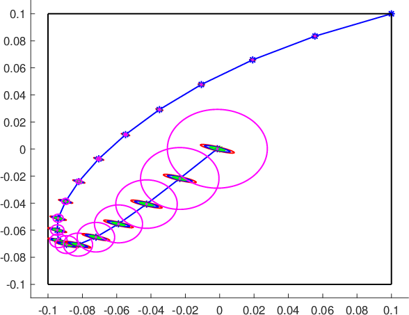
Refer to caption
Fig. 5: Initially predicted open-loop trajectory x⋅|0∗x^{*}_{\cdot|0} (blue), tube 𝕏⋅|0∗\mathbb{X}_{\cdot|0}^{*} via Prop. 5 (red), its adaptive one (green), tube via Prop. 4 (blue), the Lipschitz based approach [12] (c.f. Sec. III-F) (magenta), state constraints (black).

Closed loop performance

To compare the performance improvement relative to a purely robust MPC formulation (without parameter estimation), we consider a prediction horizon of N=12N=12 and repeatedly reinitialize the system at initial points x0=(0.1,0.1)x_{0}=(0.1,0.1) and x0=(−0.1,−0.1)x_{0}=(-0.1,-0.1) (without reinitializing the parameter updates) and then simulate the system over T=50T=50 steps. The difference in performance due to the LMS update can be seen in Figure 6. There, we can a robust MPC formulation (without parameter adaptation), the proposed RAMPC starting at t=0t=0 and also the proposed RAMPC reinitialized at x0x_{0} after multiple runs of being reinitialized and thus continuously improving the parameter estimates. We can see that the main difference due to improved parameter estimation is already visible at t=5t=5. Compared to the robust formulation without adaptation, the RAMPC formulation decreases the overshoot. Considering the cost ∑t=0T−1ℓ⁡(xt,ut)\sum_{t=0}^{T-1}\ell(x_{t},u_{t}) with T=50T=50, we can see a relative performance improvement of 3.5%3.5~\% by utilizing the LMS update. This performance improvement is expected to increase for larger parametric uncertainty.
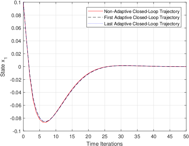
Refer to caption
Fig. 6: Closed-Loop Trajectories with x0=(0.1,0.1)x_{0}=(0.1,0.1): Robust MPC (without parameter adaptation) (red, solid), RAMPC trajectory (black, dashed) and RAMPC trajectory after multiple simulations (blue, dotted), i.e., for t∈[400,450]t\in[400,450].