$H_{\infty}$ Model-free Reinforcement Learning
with Robust Stability Guarantee

Minghao HanDepartment of Control Science and EngineeringHarbin Institute of Technologymhhan@hit.edu.cnYuan TianDepartment of Cognitive RoboticsDelft University of Technologyy.tian-8@student.tudelft.nlLixian ZhangDepartment of Control Science and EngineeringHarbin Institute of Technologylixianzhang@hit.edu.cnJun WangDepartment of Computer ScienceUniversity College Londonjun.wang@cs.ucl.ac.uk Wei PanDepartment of Cognitive RoboticsDelft University of Technologywei.pan@tudelft.nl

Abstract

Reinforcement learning is showing great potentials in robotics applications, including autonomous driving, robot manipulation and locomotion. However, with complex uncertainties in the real-world environment, it is difficult to guarantee the successful generalization and sim-to-real transfer of learned policies theoretically. In this paper, we introduce and extend the idea of robust stability and $H_{\infty}$ control to design policies with both stability and robustness guarantee. Specifically, a sample-based approach for analyzing the Lyapunov stability and performance robustness of a learning-based control system is proposed. Based on the theoretical results, a maximum entropy algorithm is developed for searching Lyapunov function and designing a policy with provable robust stability guarantee. Without any specific domain knowledge, our method can find a policy that is robust to various uncertainties and generalizes well to different test environments. In our experiments, we show that our method achieves better robustness to both large impulsive disturbances and parametric variations in the environment than the state-of-art results in both robust and generic RL, as well as classic control. Anonymous code is available to reproduce the experimental results at https://github.com/RobustStabilityGuaranteeRL/RobustStabilityGuaranteeRL.

^†^†footnotetext:

*

for correspondence.

1 Introduction

As a powerful learning control paradigm, reinforcement learning is extremely suitable for finding the optimal policy in tasks where the dynamics are either unknown or affected by severe uncertainty (Buşoniu et al. 2018). Its combination with the deep neural network has boosted applications in autonomous driving (Sallab et al. 2017), complicated robot locomotion Hwangbo et al. 2019, and skilful games like Atari (Mnih et al. 2015) and Go (Silver et al. 2017). However, overparameterized policies are prone to become overfitted to the specific training environment, limiting its generalization to the various scenarios Pinto et al. 2017. Additionally, RL agents trained in simulation, though cheap to obtain, but likely suffer from the reality gap problem Koos et al. 2010 when transferred from virtual to the real world. To overcome these drawbacks, various efforts are made to enhance the robustness of the policy Jakobi et al. 1995; Tobin et al. 2017; Mordatch et al. 2015, since a robust policy has a greater chance of successful generalization and transfer.

Contribution In this paper, we propose a unified framework of designing policies with both stability and robust performance guarantee against the various uncertainties in the environment. Without any specific domain knowledge, our method is able to find policy that is robust to large exogenous disturbances and generalizes well to different test environment. First, a novel model-free method for analyzing the Lyapunov stability and $H_{\infty}$ performance of the closed-loop system is developed. Based on the theoretical results, we propose the Robust Lyapunov-based Actor-Critic (RLAC) algorithm to simultaneously find the Lyapunov function and policy that can guarantee the robust stability of the closed-loop system. We evaluate RLAC on a simulated cartpole in the OpenAI gym (Brockman et al. 2016) environment and show that our approach is robust to: i) Large impulsive disturbance: The trained agent is able to recover when disturbed by adversary impulses 4-6 times of the maximum control input, while other baselines fail almost surely. ii) Parametric Uncertainty: The learned policy generalizes better than the baselines to different test environment settings (e.g. different mass and structural values).

2 Preliminaries

2.1 Markov Decision Process and Reinforcement Learning

A Markov decision process (MDP) is a tuple, ( $S,A,c,P,\rho$ ), where $S$ is the set of states, $A$ is the set of actions, $c(s,a)\in[0,\infty)$ is the cost function, $P(s^{\prime}|s,a)$ is the transition probability function, and $\rho(s)$ is the starting state distribution. $\pi(a|s)$ is a stationary policy denoting the probability of selecting action $a$ in state $s$ . In addition, the cost function under stationary policy is defined as $c_{\pi}(s)\doteq\mathbb{E}_{a\sim\pi}c(s,a)$ .

In this paper, we divide the state $s$ into two vectors, $s^{1}$ and $s^{2}$ , where $s^{1}$ is composed of elements of $s$ that are aimed at tracking the reference signal $r$ while $s^{2}$ contains the rest. The cost function is defined as $\|s^{1}-r\|$ , where $\|\cdot\|$ denotes the Euclidean norm.

2.2 Robust Control Against Environment Uncertainty

Definition 1.

The stochastic system is said to be stable in mean cost if $\lim_{t\rightarrow\infty}\mathbb{E}_{s_{t}}c_{\pi}(s_{t})=0$ holds for any initial condition $s_{0}\in\{s_{0}|c_{\pi}(s_{0})\leq b\}$ . If $b$ is arbitrarily large then the stochastic system is globally stable in mean cost.

To address the performance of the agent in the presence of uncertainty, the following definition is needed.

Definition 2.

The system is said to be mean square stable (MSS) with an $l_{2}$ gain less or equal than $\eta$ , if the system is MSS when $w=0$ , and the following holds for all $w\in l_{2}[0,+\infty)$ ,

\sum_{t=0}^{\infty}\mathbb{E}_{s_{t}}c_{\pi}(s_{t})\leq\sum_{t=0}^{\infty}\mathbb{E}_{s_{t}}\eta^{2}\|w(s_{t})\|_{2}

(1)

where $\eta\in\mathbb{R}_{+}$ . $z(s_{t})$ is the error output of the system and $w(s_{t})$ is the uncertainty, which is composed of both environmental disturbance and modelling error.

The robust performance guarantee (1) holds for all $w$ , is equivalent to guaranteeing the inequality for the worst case induced by $w$ , i.e.,

\sup_{w}\sum_{t=0}^{\infty}\mathbb{E}_{s_{t}}c_{\pi}(s_{t})-\eta^{2}\|w(s_{t})\|_{2}\leq 0

(2)

3 Main Results

3.1 Lyapunov-based $H_{\infty}$ Learning Control

In this section, we propose the main assumptions and a new theorem.

Assumption 1.

The stationary distribution of state $q_{\pi}(s)\triangleq\lim_{t\rightarrow\infty}P(s|\rho,\pi,t)$ exists.

Assumption 2.

There exists a positive constant $b$ such that $\rho(s)>0,\forall s\in\{s|c_{\pi}(s)\leq b\}$ .

The core theoretical results on analyzing the stability and robust performance of the closed-loop system with the help of Lyapunov function and sampled data are presented. The Lyapunov function is a class of continuously differentiable semi-positive definite functions $L:\mathcal{S}\to\mathbb{R}_{+}$ . The general idea of exploiting Lyapunov function is to ensure that the derivative of Lyapunov function along the state trajectory is semi-negative definite so that the state goes in the direction of decreasing the value of Lyapunov function and eventually converges to the set or point where the value is zero.

Theorem 1.

If there exists a continuous differentiable function $L:\mathcal{S}\rightarrow\mathbb{R}_{+}$ and positive constants $\alpha_{1}$ , $\alpha_{2}$ , $\alpha_{3},\eta,k_{1},k_{2}$ such that

	$\displaystyle\alpha_{1}c_{\pi}\left(s\right)\leq L(s)\leq\alpha_{2}c_{\pi}\left(s\right)$		(3)
	$\displaystyle\mathbb{E}_{\beta(s)}(\mathbb{E}_{s^{\prime}\sim P_{\pi}}L(s^{\prime})-L(s))<\mathbb{E}_{\beta(s)}[\eta\\|w(s)\\|-(\alpha_{3}+1)c_{\pi}\left(s\right)]$		(4)

holds for all $\{\rho|\mathbb{E}_{s_{0}\sim\rho}c_{\pi}(s_{0})\leq k_{1}\}$ and $\{w|\|w\|\leq k_{2}\}$ . $\beta_{\pi}(s)\triangleq\lim_{N\rightarrow\infty}\frac{1}{N}\sum_{t=0}^{N}P(s_{t}=s|\rho,\pi,t)$ is the sampling distribution. Then the system is mean square stable and has $l_{2}$ gain no greater than $\eta/(\alpha_{3}+1)$ . If the above holds for $\forall k_{1},k_{2}\in\mathbb{R}_{+}$ , then the system is globally mean square stable with finite $l_{2}$ gain.

Proof of Theorem 1 is given in Appendix A.

3.2 Learning the Adversarial Disturber

In our setting, in addition to the control policy $\pi$ , a disturber policy $\mu(w|s)$ is introduced to actively select the worst disturbance for a given state. More specifically, the adversarial disturber seeks to find the disturbance input $w$ over which the system has the greatest $l_{2}$ gain, i.e. maximizing the following cost function,

\max_{\theta_{\mu}}J(\mu)=\mathbb{E}_{\beta(s),\mu(w|s)}(c_{\pi}(s)-\eta^{2}\|w\|)

(5)

where $\theta_{\mu}$ is the parameter of the disturber policy $\mu$ .

4 Algorithm

In this section, based on the theoretical results in Section 3, we propose an actor-critic style algorithm with robust stability guarantee (RLAC).

In this algorithm, we include a critic Lyapunov function $L_{c}$ to provide the policy gradient, which satisfies $L(s)=\mathbb{E}_{a\sim\pi}L_{c}(s,a)$ . Through Lagrangian method, the objective function for $\pi$ is obtained as follow,

	$\displaystyle J(\pi)$	$\displaystyle=\mathbb{E}_{(s,a,w,c,s^{\prime})\sim\mathcal{D}}\left[\beta\log(\pi(f_{\theta_{\pi}}(\epsilon,s)\|s))+\lambda\Delta L(s,a,w,c,s^{\prime})\right]$		(6)
	$\displaystyle\Delta L(s,a,w,c,s^{\prime})$	$\displaystyle=\left(L_{c}(s^{\prime},f_{\theta_{\pi}}(\epsilon,s^{\prime}))-L_{c}(s,a)+(\alpha_{3}+1)c-\eta^{2}\\|w\\|_{2}\right)$		(6)

where $\pi$ is parameterized by a neural network $f_{\theta_{\pi}}$ and $\epsilon$ is an input vector consisted of Gaussian noise. In the above objective, $\nu$ and $\lambda$ are the positive Lagrangian multipliers, of which the values are adjusted automatically. The gradient of (6) with respect to the policy parameter $\theta_{\pi}$ is approximated by

\nabla_{\theta}J(\pi)=\mathbb{E}_{\mathcal{D}}\left[\nabla_{\theta}\nu\log(\pi_{\theta}(a|s))+\nabla_{a}\nu\log(\pi_{\theta}(a|s))\nabla_{\theta}f_{\theta}(\epsilon,s)+\lambda\nabla_{a^{\prime}}L_{c}(s^{\prime},a^{\prime})\nabla_{\theta}f_{\theta}(\epsilon,s^{\prime})\right]

(7)

The Lyapunov function is updated through minimizing the following objective

\displaystyle J(L_{c})=\mathbb{E}_{(s,a)\sim\mathcal{D}}\left[\frac{1}{2}(L_{c}(s,a)-L_{\text{target}}(s,a))^{2}\right]

(8)

We use the sum of cost over a finite time horizon $N$ as the Lyapunov candidate, i.e.

\displaystyle L_{\text{target}}(s,a)=\sum_{t=t_{0}}^{N}c(s_{t},a_{t})

(9)

which has long been exploited as the Lyapunov function in establishing the stability criteria for model predictive control (MPC) (Mayne et al. 2000). The pseudo-code of RLAC is presented in Algorithm 1.

5 Experimental Results

In this section, we evaluate the robustness of RLAC against i) large impulsive disturbances; ii) parametric uncertainty. Setup of the experiment is referred to Appendix C.

5.1 Robustness to Impulsive Disturbances

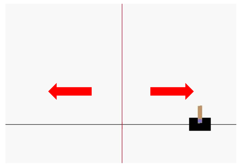
Refer to caption — (a) Visualization of the disturbance

We evaluate the robustness of the agents trained by RLAC and baselines against unseen exogenous disturbance. We measure the robust performance via the death rate, i.e., the probability of pole falling after impulsive disturbance. As observed in the figure, RLAC gives the most robust policy against the impulsive force. It maintains the lowest death rate throughout the experiment, far more superior than SAC and RARL. Moreover, RLAC performs even better than MPC and LQR, which possess the full information of the model and are available.

5.2 Robustness to Parametric Uncertainty

In this experiment, we evaluate the trained policies in environments with different parameter settings. In the training environment, the parameter length of pole $l=0.5$ and mass of cart $m_{c}=1$ , while during evaluation $l$ and $m_{c}$ are selected in a 2-D grid with $l\in[0.2,2.0]$ and $m_{c}\in[0.4,2.0]$ .

As shown in the heat maps in Figure 2, RLAC achieves the lowest death rate (zero for the majority of the parameter settings) and obtains reasonable total cost (lower than 100). The total cost of RLAC is slightly higher than SAC and RARL since the agents hardly die and sustain longer episodes. Compared to SAC, RARL achieves lower death rate and comparable total cost performance. LQR performs well in the region where parameters are close to the nominal model but deteriorates soon as parameters vary. All of the model-free methods outperform LQR in terms of robustness to parametric uncertainty, except for the case of low $l$ and $m_{c}$ (left bottom of the grid). This is potentially due to the overparameterized policy does not generalize well to the model where dynamic is more sensitive to input than the one used for training.

References

Buşoniu et al. [2018] Lucian Buşoniu, Tim de Bruin, Domagoj Tolić, Jens Kober, and Ivana Palunko. Reinforcement learning for control: Performance, stability, and deep approximators. Annual Reviews in Control, 2018.
Sallab et al. [2017] Ahmad EL Sallab, Mohammed Abdou, Etienne Perot, and Senthil Yogamani. Deep reinforcement learning framework for autonomous driving. Electronic Imaging, 2017(19):70–76, 2017.
Hwangbo et al. [2019] Jemin Hwangbo, Joonho Lee, Alexey Dosovitskiy, Dario Bellicoso, Vassilios Tsounis, Vladlen Koltun, and Marco Hutter. Learning agile and dynamic motor skills for legged robots. Science Robotics, 4(26):eaau5872, 2019.
Mnih et al. [2015] Volodymyr Mnih, Koray Kavukcuoglu, David Silver, Andrei A Rusu, Joel Veness, Marc G Bellemare, Alex Graves, Martin Riedmiller, Andreas K Fidjeland, Georg Ostrovski, et al. Human-level control through deep reinforcement learning. Nature, 518(7540):529, 2015.
Silver et al. [2017] David Silver, Julian Schrittwieser, Karen Simonyan, Ioannis Antonoglou, Aja Huang, Arthur Guez, Thomas Hubert, Lucas Baker, Matthew Lai, Adrian Bolton, et al. Mastering the game of go without human knowledge. Nature, 550(7676):354, 2017.
Pinto et al. [2017] Lerrel Pinto, James Davidson, Rahul Sukthankar, and Abhinav Gupta. Robust adversarial reinforcement learning. In Proceedings of the 34th International Conference on Machine Learning-Volume 70, pages 2817–2826. JMLR. org, 2017.
Koos et al. [2010] Sylvain Koos, Jean-Baptiste Mouret, and Stéphane Doncieux. Crossing the reality gap in evolutionary robotics by promoting transferable controllers. In Proceedings of the 12th annual conference on Genetic and evolutionary computation, pages 119–126. ACM, 2010.
Jakobi et al. [1995] Nick Jakobi, Phil Husbands, and Inman Harvey. Noise and the reality gap: The use of simulation in evolutionary robotics. In European Conference on Artificial Life, pages 704–720. Springer, 1995.
Tobin et al. [2017] Josh Tobin, Rachel Fong, Alex Ray, Jonas Schneider, Wojciech Zaremba, and Pieter Abbeel. Domain randomization for transferring deep neural networks from simulation to the real world. In 2017 IEEE/RSJ International Conference on Intelligent Robots and Systems (IROS), pages 23–30. IEEE, 2017.
Mordatch et al. [2015] Igor Mordatch, Kendall Lowrey, and Emanuel Todorov. Ensemble-cio: Full-body dynamic motion planning that transfers to physical humanoids. In 2015 IEEE/RSJ International Conference on Intelligent Robots and Systems (IROS), pages 5307–5314. IEEE, 2015.
Brockman et al. [2016] Greg Brockman, Vicki Cheung, Ludwig Pettersson, Jonas Schneider, John Schulman, Jie Tang, and Wojciech Zaremba. Openai gym. arXiv preprint arXiv:1606.01540, 2016.
Mayne et al. [2000] David Q Mayne, James B Rawlings, Christopher V Rao, and Pierre OM Scokaert. Constrained model predictive control: Stability and optimality. Automatica, 36(6):789–814, 2000.
Royden [1968] Halsey Lawrence Royden. Real analysis. Krishna Prakashan Media, 1968.
Haarnoja et al. [2018] Tuomas Haarnoja, Aurick Zhou, Pieter Abbeel, and Sergey Levine. Soft actor-critic: Off-policy maximum entropy deep reinforcement learning with a stochastic actor. arXiv preprint arXiv:1801.01290, 2018.

Appendix A Proof of Theorem 1

Proof.

The existence of sampling distribution $\mu_{\pi}(s)$ is guaranteed by the existence of $q_{\pi}(s)$ (Assumption 1). Since the sequence $\{P(s|\rho,\pi,t),t\in\mathbb{Z}_{+}\}$ converges to $q_{\pi}(s)$ as $t$ approaches $\infty$ , then by the Abelian theorem, the sequence $\{\frac{1}{N}\sum_{t=0}^{N}P(s|\rho,\pi,t),N\in\mathbb{Z}_{+}\}$ also converges and $\mu_{\pi}(s)=q_{\pi}(s)$ . Combined with the form of $\mu_{\pi}$ , Eq.(4) infers that

\displaystyle\int_{\mathcal{S}}\lim_{N\rightarrow\infty}\frac{1}{N}\sum_{t=0}^{N}P(s|\rho,\pi,t)(\mathbb{E}_{P_{\pi}(s^{\prime}|s)}L(s^{\prime})-L(s))\mathrm{d}s<\mathbb{E}_{\beta(s)}[\eta\|w(s)\|-(\alpha_{3}+1)c_{\pi}\left(s\right)]

(10)

First, the stability of the system in mean cost will be proved. According to Eq.(3), $L(s)\leq\alpha_{2}c_{\pi}(s)$ for all $s\in\mathcal{S}$ and consider that $P(s|\rho,\pi,t)\leq 1$ ,

P(s|\rho,\pi,t)L(s)\leq\alpha_{2}c_{\pi}\left(s\right),\forall s\in\mathcal{S},\forall t\in\mathbb{Z}_{+}

On the other hand, the sequence $\{\frac{1}{N}\sum_{t=0}^{N}P(s|\rho,\pi,t)L(s),N\in\mathbb{Z}_{+}\}$ converges pointwise to the function $q_{\pi}(s)L(s)$ . According to the Lebesgue’s Dominated convergence theorem[Royden 1968], if a sequence ${f_{n}(s)}$ converges pointwise to a function $f$ and is dominated by some integrable function $g$ in the sense that,

|f_{n}(s)|\leq g(s),\forall s\in\mathcal{S},\forall n

Then

\lim_{n\rightarrow\infty}\int_{\mathcal{S}}f_{n}(s)\mathrm{d}s=\int_{\mathcal{S}}\lim_{n\rightarrow\infty}f_{n}(s)\mathrm{d}s

Thus the left hand side of Eq.(10)

		$\displaystyle\int_{\mathcal{S}}\lim_{N\rightarrow\infty}\frac{1}{N}\sum_{t=0}^{N}P(s\|\rho,\pi,t)(\int_{\mathcal{S}}P_{\pi}(s^{\prime}\|s)L(s^{\prime})\mathrm{d}s^{\prime}-L(s))\mathrm{d}s$
	$\displaystyle=$	$\displaystyle\lim_{N\rightarrow\infty}\frac{1}{N}(\sum_{t=1}^{N+1}\mathbb{E}_{P(s\|\rho,\pi,t)}L(s)-\sum_{t=0}^{N}\mathbb{E}_{P(s\|\rho,\pi,t)}L(s))$
	$\displaystyle=$	$\displaystyle\lim_{N\rightarrow\infty}\frac{1}{N}\left(\mathbb{E}_{P(s\|\rho,\pi,N+1)}L(s)-\mathbb{E}_{\rho(s)}L(s)\right)$

First, when $w(s)\equiv 0$ , Eq.(10) infers

\lim_{N\rightarrow\infty}\frac{1}{N}\left(\mathbb{E}_{P(s|\rho,\pi,N+1)}L(s)-\mathbb{E}_{\rho(s)}L(s)\right)<-(\alpha_{3}+1)\lim_{t\rightarrow\infty}\mathbb{E}_{P(s|\rho,\pi,t)}c_{\pi}\left(s\right)

(11)

Since $\mathbb{E}_{\rho(s)}L(s)$ is a finite value and $L$ is semi-positive definite, it follows that

\lim_{t\rightarrow\infty}\mathbb{E}_{P(s|\rho,\pi,t)}c_{\pi}\left(s\right)\leq\lim_{N\rightarrow\infty}\frac{1}{N}(\frac{1}{\alpha_{3}+1}\mathbb{E}_{\rho(s)}L(s))=0

(12)

Suppose that there exists a state $s_{0}\in\{s_{0}|c_{\pi}(s_{0})\leq b\}$ such $\lim_{t\rightarrow\infty}\mathbb{E}_{P(s|s_{0},\pi,t)}c_{\pi}\left(s\right)=c$ , $c>0$ or $\lim_{t\rightarrow\infty}\mathbb{E}_{P(s|s_{0},\pi,t)}c_{\pi}\left(s\right)=\infty$ . Consider that $\rho(s_{0})>0$ for all starting states in $\{s_{0}|c_{\pi}(s_{0})\leq b\}$ (Assumption 2), then $\lim_{t\rightarrow\infty}\mathbb{E}_{s_{t}\sim P(\cdot|\pi,\rho)}c_{\pi}\left(s_{t}\right)>0$ , which is contradictory with Eq.(12). Thus $\forall s_{0}\in\{s_{0}|c_{\pi}(s_{0})\leq b\}$ , $\lim_{t\rightarrow\infty}\mathbb{E}_{P(s|s_{0},\pi,t)}c_{\pi}\left(s\right)=0$ . Thus the system is stable in mean cost by Definition 1.

Next, the $H_{\infty}$ performance of the system will be proved. When $w(s)\neq 0$ , Eq.(10) infers

\lim_{N\rightarrow\infty}\frac{1}{N}\left(\mathbb{E}_{P(s|\rho,\pi,N+1)}L(s)-\mathbb{E}_{\rho(s)}L(s)\right)<\mathbb{E}_{\beta(s)}[\eta\|w(s)\|-(\alpha_{3}+1)c_{\pi}\left(s\right)]

(13)

Since $\mathbb{E}_{\rho(s)}L(s)$ is a finite and Due to the semi-definiteness of $c_{\pi}$ and $\mathbb{E}_{P(s|\rho,\pi,N+1)}L(s)$ is semi-positive definite, one has

\displaystyle\lim_{N\rightarrow\infty}\frac{1}{N}\sum_{t=0}^{N}\mathbb{E}_{P(s|\rho,\pi,t)}\left[\left(\alpha_{3}+1\right)c_{\pi}\left(s\right)-\eta\|w(s)\|\right]

\displaystyle<0

(14)

The above inequality only holds if $\sum_{t=0}^{\infty}\mathbb{E}_{P(s|\rho,\pi,t)}\left[\left(\alpha_{3}+1\right)c_{\pi}\left(s\right)-\eta\|w(s)\|\right]<0$ , thus the system has $l_{2}$ gain less than $\frac{\eta}{\alpha_{3}+1}$ , which concludes the proof. ∎

Appendix B Algorithm

Algorithm 1 Robust Lyapunov-based Actor Critic (RLAC)

Initialize replay buffer

R

and the Lagrangian multiplier

\lambda

\beta

, learning rate

\alpha

Randomly initialize Lyapunov critic network

L_{c}(s,a)

, actor

\pi(a|s)

, disturber

\mu(d|s)

with parameters

\phi_{L_{c}}

\theta_{\pi}

\theta_{\mu}

Initialize the parameters of target networks with

\overline{\phi}_{L_{c}}\leftarrow\phi_{L_{c}}

\overline{\theta}_{\pi}\leftarrow\theta_{\pi}

for each iteration do

Sample

s_{0}

according to

\rho

for

t

N_{c}

Sample

a_{t}

from

\pi_{a}(s)

and

d_{t}

from

\pi_{d}(s)

and step forward

Observe

s_{t+1}

c_{t}

and store

(s_{t},a_{t},d_{t},c_{t},s_{t+1})

R

end for

for

i

N_{u}

Sample minibatches of

N

transitions from

R

Estimate policy gradient:

	$\displaystyle\phi_{L_{c}}$	$\displaystyle\leftarrow\phi_{L_{c}}+\alpha\nabla_{\phi_{L_{c}}}J(L_{c})$
	$\displaystyle\theta_{\pi}$	$\displaystyle\leftarrow\theta_{\pi}+\alpha\nabla_{\theta_{\pi}}J(\pi)$
	$\displaystyle\theta_{\mu}$	$\displaystyle\leftarrow\textit{PolicyOptimizer}(J(\pi_{\mu}))$

Update Lagrangian multipliers

\lambda

\beta

and the parameter of target networks,

\overline{\phi}_{L_{c}}

\overline{\theta}_{\pi}

end for

Appendix C Experiment Setup

Figure 3: Cumulative cost curves for RLAC, RARL and SAC; the shadowed region shows the 1-SD confidence interval over 10 random seeds and the X-axis indicates the total time steps in thousand.

We compare with robust adversarial reinforcement learning (RARL, [Pinto et al. 2017]) which is considered to be the model-free robust RL baseline. RARL demonstrated great robustness to both exogenous disturbance and parametric disturbance on a series of continuous control tasks. In the implementation of RARL Pinto et al. 2017, TRPO was used as the policy optimizer, though other policy optimization methods are also comparable with the framework. Without loss of generality, we use soft actor-critic (SAC) [Haarnoja et al. 2018] as the policy optimizer for RARL, given that both sample efficiency and final performance of SAC exceeds the state of art on a series of continuous control benchmarks. We also include SAC as the generic RL baseline. Linear Quadratic Regulator (LQR) and MPC are included as the model-based baseline, which is guaranteed to find the optimal analytic solution given the well established linear model and weighting matrices. Hyperparameters and other details for the implementation of RLAC are referred to Appendix D.

We evaluate RLAC and baselines on a simulated cartpole in the OpenAI gym environment (all the units are dimensionless), details of the environment is referred to Appendix C. The agent is expected to sustain the pole vertically at $x=0$ . Both the RLAC and baseline agents are trained under the static environment setting, i.e., with unchanged model parameters and dynamics, and evaluated in the environment variants with unseen uncertainty. During training, both RLAC and RARL generate disturbance input to affect the performance of the policy. The cost and state at the next step are determined by the action and disturbance jointly. The magnitude of the disturbances is held no larger than $5$ , while the actions are below $20$ .

Each algorithm is trained for the same amount of global time steps over $10$ random seeds with optimized hyperparameters. The total cost of rollouts during training is shown in Figure 3. As shown in the figure, all the algorithms converge eventually, achieving similar final performance in terms of return.

In the cartpole experiment, the agent is to sustain the pole vertically at the central position. This is a modified version of cartpole in Brockman et al. 2016 with continuous action space. The action is the horizontal force on the cart( $F\in[-20,20]$ ). The position $x$ is limited to $(-x_{\text{threshold}},x_{\text{threshold}})$ , $x_{\text{threshold}}=10$ . $\theta$ is the angle position with respect to the vertical direction, $\theta\in(-\theta_{\text{threshold}},\theta_{\text{threshold}})$ where $\theta_{\text{threshold}}=0.349\textit{ rad}$ . The cost function $c=(\frac{x}{x_{\text{threshold}}})^{2}+20(\frac{\theta}{\theta_{\text{threshold}}})^{2}$ . The agent is initialized randomly between $x\in[-5,5]$ while other variables initialized in $[-0.2,0.2]$ . The maximum length of episodes is 250.

C.1 Robustness to Impulsive Disturbances

We evaluate the robustness of the agents trained by RLAC and baselines against unseen exogenous disturbance. To show this, we implement an impulsive adversarial force on the cartpole, ranging from 80 to 120 which is far more larger than the maximum action input and disturbance during training. The impulsive disturbance is analogous to a sudden hit or strong wind applied on the cart. The disturbance acts in the direction of pushing the cart away from the origin, as shown in Figure 1 (a), and only takes place at the $100$ th time step.

We use the death rate instead of total cost because the failure will end the episode in advance and result in a rather low total cost. Under different impulse magnitudes, the policies trained by RLAC and baselines over different initializations are evaluated for 500 times, and results are shown in 1 (b).

C.2 Robustness to Parametric Uncertainty

The trained agents with different initializations are evaluated with an equal number of episodes, and at each point of the parameter grid, the agents are evaluated for 100 times. For the same reason discussed in the previous subsection, total cost together with death rate are shown in Figure 2 to demonstrate the robustness of RLAC and baselines.

Appendix D Hyperparameters

Hyperparameters	Value
Minibatch size	256
Actor learning rate	1e-4
Lyapunov learning rate	3e-4
Time horizon $N$	10
$N_{c}$	150
$N_{u}$	50
Target entropy	-1
Soft replacement( $\tau$ )	0.005
Discount( $\gamma$ )	0.995
$\eta$	1
$\alpha_{3}$	1

Table 1: RLAC Hyperparameters

For the policy network, we use a fully-connected MLP with two hidden layers of 64 units, and ReLU nonlinearities, outputting the mean and standard deviations of a Gaussian distribution. For the Lyapunov network, we use a fully-connected MLP with two hidden layers of 64 units, and ReLU nonlinearity respectively, outputting the Lyapunov value. We adopt the same invertible squashing function technique as Haarnoja et al. 2018 to the output layer of policy network.

		$\displaystyle\int_{\mathcal{S}}\lim_{N\rightarrow\infty}\frac{1}{N}\sum_{t=0}^{N}P(s\|\rho,\pi,t)(\int_{\mathcal{S}}P_{\pi}(s^{\prime}\|s)L(s^{\prime})\mathrm{d}s^{\prime}-L(s))\mathrm{d}s$
	$\displaystyle=$	$\displaystyle\lim_{N\rightarrow\infty}\frac{1}{N}(\sum_{t=1}^{N+1}\mathbb{E}_{P(s\|\rho,\pi,t)}L(s)-\sum_{t=0}^{N}\mathbb{E}_{P(s\|\rho,\pi,t)}L(s))$
	$\displaystyle=$	$\displaystyle\lim_{N\rightarrow\infty}\frac{1}{N}\left(\mathbb{E}_{P(s\|\rho,\pi,N+1)}L(s)-\mathbb{E}_{\rho(s)}L(s)\right)$

H∞H_{\infty} Model-free Reinforcement Learning with Robust Stability Guarantee