Geometry and flexibility of optimal catalysts in a minimal elastic network model
Abstract
We have a general knowledge of the principles by which catalysts accelerate the rate of chemical reactions but no precise understanding of the geometrical and physical constraints to which their design is subject. To analyze these constraints, we introduce a minimal model of catalysis based on elastic networks where the implications of the geometry and flexibility of a catalyst can be studied systematically. The model demonstrates the relevance and limitations of the principle of transition-state stabilization: optimal catalysts are found to have a geometry complementary to the transition state but a degree of flexibility that non-trivially depends on the parameters of the reaction as well as on external parameters such as the concentrations of reactants and products. The results illustrate how simple physical models can provide valuable insights on the design of catalysts.
Catalysts, which increase the rate of chemical reactions without being part of their products, are essential to biological processes as well as to the industrial production of most chemicals. We have a general theory of catalysis, transition-state theory Eyring:1935te; Evans:1935dg, and detailed knowledge of the mechanisms by which many catalysts operate, in particular enzymes fersht1999structure. We also have an increasing capacity to model and numerically simulate catalytic processes at an atomic level karplus2002molecular. Yet, basic questions pertaining to the existence of fundamental geometrical and physical constraints to catalysis are still the object of speculations: To what extent does efficient catalysis require catalysts to be rigid? Kraut:1988th Or thermally stable? karshikoff2015rigidity Does it impose a minimal size on catalysts? Srere:1984wf Is catalysis subject to a general rate-accuracy trade-off? tawfik2014accuracy
Answers to such questions would help us uncovering the design principles of natural enzymes davidi2018bird, directing the experimental evolution of novel enzymes goldsmith2012directed, and clarifying the conditions under which life can emerge walker2017re.
Missing is a theoretical framework that is sufficiently elaborate to account for geometric and physical constraints, yet sufficiently simple to allow for a systematic comparison of varied geometries and physical designs. For this purpose, the low-dimensional phase-space formulation of transition-state theory is too abstract, as it does not refer explicitly to the spatial architecture of catalysts. The atom-level description of models studied by molecular dynamic simulations is, on the other hand, too detailed, as it prohibits computational exploration of a large number of architectures.
An alternative lies in the simplified physical models developed to study properties of proteins other than catalysis, notably folding Pande:1997cp, binding Miller:1997es and allostery eckmann2019colloquium. Particularly insightful are elastic network models, which approximate molecules by a network of beads interacting through elastic springs Chennubhotla:2005bb. In their different guises, these models have provided conceptual and quantitative insights into several features of proteins, including thermal fluctuations bahar1997direct, conformational changes tama2001conformational, unfolding kinetics Dietz:2008gj; Srivastava:2013hy, specificity Savir:2007bd; rivoire2018minimal and allostery McLeish:2013ij; yan2017architecture.
Here we propose to adapt the framework of elastic network models to study catalysis. We illustrate this proposal by defining and solving a one-dimensional model of catalysis. Our model may be viewed as a reformulation and systematic analysis of a model of strain-induced catalysis first suggested by Haldane haldane1930enzymes and later partly formalized by Gavish Gavish:1978vr; Gavish86; Bustamante:2004fo. While deliberately minimal, the model addresses a key design challenge: an efficient catalyst must stabilize the transition state of the reaction to accelerate it but also bind to the reactant and release the product. These conflicting demands lead to non-trivial constraints on flexibility, which our model recapitulates. The model also demonstrates how the optimal design of a catalyst depends, beyond the mechanisms of the reaction, on the conditions under which catalysis occurs. Our analysis is limited to one dimension but the model is straightforward to extend, if not to solve, in two or three dimensions. Our approach thus complements other bottom-up studies of catalysis Gavish:1978vr; Zeravcic:cm towards a better understanding of the geometrical and physical constraints to which proficient catalysts are subject.
I General framework
Analyzing the physical and geometrical constraints to efficient catalysis requires a physical model that specifies the range of designs to be examined and a criterion to quantify catalytic efficiency. Our choices in defining such a model are guided by a principle of simplicity, the goal being to obtain a physically coherent framework where a large number of different architectures can effectively be explored and compared.
I.1 Physical model
Elastic network models are one of the simplest physical models where geometry, strain and energy can be related. They consist of beads interacting through elastic springs and have been extensively used to study the internal motions of proteins Chennubhotla:2005bb. Each spring is characterized by two parameters, a spring constant and a free length. Varying the number of beads and the parameters of the springs that connect them allows for the sampling of a large number of designs, including networks approximating three-dimensional protein structures Chennubhotla:2005bb. Here, we propose to describe not only a catalyst, but also its substrate and their interaction within a common elastic network model. To this end, we assume that each spring has a maximal extension above which it breaks and below which it reforms. More precisely, each spring contributes to the total energy by if the extension satisfies and 0 if , where is the spring constant, the free length and the maximal extension. When the beads are subject to Brownian motion, which accounts for their interaction with a solvent, bonds may thus break or form as a result of thermal fluctuations.
The rupture of a bond between two beads defines an elementary chemical reaction. To have a single product as well as a single reactant, we consider a case where this rupture does not compromise the connectivity of the substrate. This is achieved by assuming that a second unbreakable bond (with infinite maximal extension) links the two beads: the presence of the two springs then defines the reactant while the absence of the breakable spring defines the product (Fig. 1, top line).
In this framework, the simplest catalyst also consists of just two beads joined by a single unbreakable spring. To describe its interaction with the substrate, either in the form of the reactant or the product , we assume that each bead of the catalyst can interact through a breakable spring with one, and only one, of the beads of the substrate (Fig. 1).
In total, our elastic network model thus comprises four beads and five springs, three of which being effectively absent if their extension exceeds a given threshold. Assuming the breakable springs to have a vanishing free length, the model is then specified by 8 parameters (Table 1).
| spring | free | maximal | |
| constant | length | extension | |
| substrate scissile bond | |||
| substrate non-scissile bond | |||
| catalyst internal bond | |||
| substrate-catalyst interaction |
I.2 Criteria for catalytic efficiency
There is no intrinsically optimal catalyst. Depending on the set-up, and not just the reaction to be catalyzed, different criteria are relevant for scoring catalytic activity. Optimizing these different criteria generally leads to different optimal designs.
Consider for instance a measure of catalytic efficiency commonly adopted in enzymology, the ratio . It assumes that the rate at which the concentration of products increases depends on the concentration of reactants and on the total concentration of catalysts by Michaelis-Menten equation cornish2014principles,
| (1) |
The ratio then characterizes the initial rate of the reaction, when . In general, however, Eq. (1) indicates that the rate depends on the concentration of reactants. The ratio should indeed be generally interpreted as a measure of specificity rather than a measure of catalytic efficiency eisenthal2007catalytic.
To see how optimizing may lead to unphysical results, consider the simplest case where Eq. (1) arises, under the scheme , where the complex is assumed to be in a quasi-steady state cornish2014principles. In this case, and . Taking , we obtain , which is independent of . Formally, can thus be made arbitrarily large by minimizing and maximizing , irrespective of , even though controls an essential step and means that no catalysis takes place. The catch is in the assumption , which underlies the choice of the ratio as a measure of catalytic efficiency. When , this assumption implies , which depends on and is certainly not satisfied when . This simple example illustrates the need to consider explicitly the concentration of reactants to obtain physically meaningful results 11 1 One could also ignore and score catalytic efficiency by but this choice would not account for the rate at which the product is generated.. As a corollary a family of optimal designs is defined, which depend on the concentration of reactants, and not just on the mechanisms of the reaction. More generally, optimal designs also depend on the concentration of products, which is assumed to be in Eq. (1).
Here, we choose to treat the concentrations and of reactants and products as two fixed parameters and to score catalytic activity by the rate at which the product is formed. This assumes a reservoir of reactants and products, so that their concentrations are constant despite the reactions that consume or produce them. This is, however, not the only possible choice. One may alternatively consider a closed-system with an initial concentration of reactants and score the concentration of products after a fixed time, or consider a chemostat with a fixed in-flow of reactants and catalysts, a fixed dilution rate and score the out-flow of products.
II Solvable one-dimensional model
The model presented in Figure 1 is defined in any dimension. We study it here in one dimension, where it has only three independent internal degrees of freedom and can be solved analytically. The details of this solution are presented in the appendices and we focus below on the results and assumptions on which they rely. While these assumptions constrain the range of examined designs, they are justified a posteriori by the finding of locally optimal designs within their range of validity.
II.1 Uncatalyzed reaction
In one dimension, a substrate is characterized by a single internal degree of freedom, the distance between its two beads, and five physical parameters, the spring constants and of the two springs that connect the two beads, their free lengths and , and the maximal extension of the breakable spring ( stands for “attractive” and for “repulsive”). Without loss of generality, we assume (Table 1). The number of parameters can be further reduced to two by considering adimensional quantities (Appendix .1).
As long as the distance between the two beads satisfies , the two springs are present and equivalent to a single spring with effective parameters
| (2) |
We assume so that a substrate with initial extension is more likely to break () than to invert the relative position of its two beads (); in this approximation, the interaction potential between the beads is harmonic (Appendix .1). For the reactant and the product to be stable, the equilibrium distance with and without the scissile bond must be respectively below and beyond the breaking point, which imposes . Additionally, we choose parameters so that the state with a broken bond is the state of lowest energy (Appendix .1 and Fig. 2).
We compute the rates of transition between states using Kramers’ escape formula kramers1940brownian, which assumes that the time scales of relaxation within each state are much smaller then the transition rates. This is valid provided barrier heights are large compared to , where is the temperature and Boltzmann’s constant (Appendix .2). This leads to the forward and reverse rates (for ) and (for ) given by
| (3) |
where . In these formulae, the unit of time is chosen so that the viscosity of the solvent and the curvature of the potential at the barrier do not appear explicitly (Appendix .2). Given these rates, the reaction is thermodynamically favored provided where and are the concentrations of the reactant and product , and where is the equilibrium constant of the reaction.
II.2 Catalysis
The catalyst is characterized by the spring constant and free length of the unbreakable spring that connects its two beads (Fig. 1). Each of these beads can interact with only one bead of the substrate and the two interactions are described by equivalent breakable springs with spring constant , free length and maximal extension (Table 1). We assume that the catalyst is rigid enough to maintain the relative position of its beads (, Appendix .3).
The system formed by the catalyst and the substrate can possibly be in states, depending on whether each of the 3 scissile bonds is broken or not. Given the equivalence between the two bonds by which the substrate and the catalyst interact, these 8 states define 6 physically distinct states (Appendix .4 and Fig. 1). These physical states are well-defined if they are associated with local minima of the potential, and we consider parameters for which this is the case (Appendix .4).
When all 6 states are well-defined, the catalysis is the result of the series of reactions
| (4) |
where the intermediate states , , , are illustrated in Figure 1. The transitions are ignored, which is justified when the rates of the uncatalyzed reaction are negligible compared to the rates of the catalyzed reaction, i.e., and . We assume and 22 2 We can always redefine the concentrations and so that it is the case. When optimizing at given values of and , however, this rescaling matters. A non-equivalent choice would for instance be to take , with representing the “cross-section” for the collision between catalysts and substrates. and obtain the other rates by application of Kramers’ escape formula (Appendix .5).
Under the assumptions that the concentrations of catalysts (under their different forms), of reactants and of products are maintained constant and that the concentrations of all intermediates are at steady state, the rate of product formation takes the form (Appendix .6)
| (5) |
The parameters of this reversible Michaelis-Menten equation cornish2014principles depend on the 8 spring parameters given in Table 1 via the rates in Eq. (4). They also depend on the temperature of the solvent but not on its viscosity, nor on the curvature of the potential near the activation barriers, which we assume to be identical for all barriers (Appendix .2).
III Optimal designs of 1D catalysts

To characterize optimal designs within the model, we maximize the reaction rate over the four parameters of the catalyst: , which characterize its flexibility and geometry, and , which characterize the strength and range of its interaction with the substrate (Table 1). The optimum generally depends on the four physical parameters of the substrate, (Table 1), on the concentrations , at which the reactant and product are present, and on the temperature of the solvent, represented by .
For the substrate, we consider the parameters of Figure 2, , , , , which correspond to parameters and for the effective bond of the reactant [Eq. (2)]. For the medium, we first consider the parameters , and . With these values, we find a locally optimal design (Fig. S2) that satisfies all the assumptions involved in the derivation of the rate : .
This solution is consistent with the proposal that an optimal catalyst must stabilize the transition state of the reaction pauling1948nature; lienhard1973enzymatic: the catalyst is maximally rigid () with a length that matches that of the transition state (). Additionally, the range of interaction is adapted to the free length of the substrate: . The value of the optimal interaction strength is, on the other hand, less obvious to interpret. It takes a finite value, contrary to what a naïve application of the principle of transition-state stabilization would predict. The optimal value of represents indeed a trade-off between the need to stabilize the transition state, which requires rigidity, and the need to release the product, which requires flexibility (Fig. 3). The energy landscape associated with this optimal design can be represented in two dimensions as a rigid catalyst with leaves only two independent internal degrees of freedom (Fig. 4).
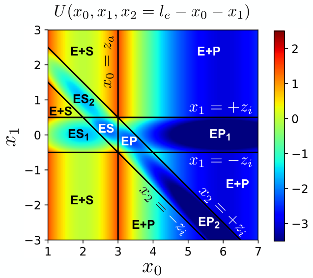
Varying the different parameters around the above values, we verify that the relationships associated with transition-state stabilization,
| (6) |
are always nearly satisfied, while is, on the other hand, parameter-dependent (Figs. S3-S4). We analyze in what follows the determinants of the optimal interaction strength assuming that the other parameters of the catalyst are given by Eq. (6).
III.1 Dependence on concentrations
Varying the concentration of reactants at vanishing concentration of products (), we find that has a non-trivial maximum that decreases with (Fig. 5). In particular, in the limit where the problem is equivalent to optimizing the specificity constant , we have : the strength of the interaction between substrate and catalyst becomes infinite. This result illustrates how optimizing the ratio can lead to unphysical designs as, in this limit, a catalyst is unable to release its product (Fig. 3).
A non-zero concentration of products () introduces an additional constraint, product inhibition. For catalysis to take place, should be small enough for the reaction to be thermodynamically favored: , where is the equilibrium constant of the uncatalyzed reaction . Under this condition, we find that is a decreasing function of both and (Fig. 6).
III.2 Dependence on physical parameters
The dependence of on the physical parameters of the substrate (Table 1) is shown in Figure 7. The results are at first sight counter-intuitive. When increasing , for instance, the activation barrier becomes higher but the interaction strength of the optimal catalyst becomes weaker. Similarly, increasing increases the activation barrier but is again associated with a smaller . On the other hand, substrates with increased or have a lower activation barrier but are associated with a larger .
To rationalize these results, note that varying or implies not only a different optimal interaction strength but, from Eq. (6), a different optimal extension and a different optimal interaction range (Figs. S3-S4). If instead of considering
| (7) |
where depends on [Eq. (2)], as in the red curve of the first panel of Figure 7, we consider
| (8) |
where is fixed, we obtain the blue curve, which is an increasing function of . Mathematically, the observation that stronger bonds are best broken by catalysts making weaker interactions with their substrate is thus explained by the difference between optimizing over a single variable versus optimizing over all variables jointly. Physically, a stronger reduces the equilibrium length of the reactant and the catalyst needs to be more flexible to bind both to this smaller reactant and to the transition state whose location is unchanged. Reasoning on just one parameter may thus be misleading because varying this parameter may have an incidence on multiple steps of the catalytic cycle and some of these effects may be compensated by varying other parameters. Mutatis mutandis, similar arguments explain the non-trivial dependence on the other parameters shown in Figure 7.

IV Discussion
We introduced a simple but general elastic network framework for studying the geometrical and physical constraints to which efficient catalysts are subject and illustrated it with the analytical solution of an elementary one-dimensional model.
The solution demonstrates the relevance and limitations of the principle of transition-state stabilization, which reduces catalysis to binding to (analogues of) the transition state of the reaction pauling1948nature; lienhard1973enzymatic. While we find that the geometry of optimal catalysts matches the geometry of the transition state, consistent with this principle, we also find that binding to this state should not be maximized. Instead, some flexibility is needed to bind to the reactant and release the product in addition to stabilize the transition state. The additional constraints that these requirements impose might explain why catalytic antibodies selected for transition-state stabilization with no consideration of product release are only modest catalysts hilvert2000critical. Binding to the reactant less than to the transition state but more than to the product, which are all chemically similar, poses a problem of fine discrimination. As previously proposed rivoire2018minimal, physical solutions to such problems can rely on a conformational switch: this is the case in the present model where the relative positions of the beads of the catalyst and the substrate are swapped during the transition (Fig. 1).
While the model is not meant to make quantitative predictions, we note that the optimal strength of interaction between substrate and catalyst is systematically larger than the strength of the bond to break; for instance, in Figure 3B, is maximal for . This is in contrast to enzymes, which can catalyze the rupture of covalent bonds by means of weaker non-covalent interactions. Introducing physical limitations on the strength and length of the various bonds may thus contribute to explain why enzymes are so large Srere:1984wf and why they make multiple interactions with their substrate. This line of reasoning was first followed by Gavish who estimated how much stress an enzyme can exert on a substrate based on a similar toy model Gavish86; his analysis, however, does not consider the full catalytic cycle and, in particular, the need for the catalyst to be flexible to release the product. Besides physical limitations, evolutionary limitations, in particular the granularity of the sequence space, may also be relevant to these questions rivoire2018minimal.
Our model captures another feature of catalysis that is likely to be very general: efficient catalysts are not only optimized for the reaction but for the conditions under which catalysis occurs. In the model, these conditions include the temperature and the concentrations of reactants and products, on which the optimal degree of flexibility depends. In another set-up, these concentrations may not be maintained constant and other parameters may be relevant, such as the concentration of catalysts or the fluctuations due to low concentrations of reactants barato2015universal.
At a physical level, approximating a molecule by an elastic network is obviously an extreme oversimplification. Enzymes, in particular, are arguably not purely mechanical devices but as importantly electronic devices. Harmonic potentials may describe small distortions of charge distributions as well as mechanical strain, but their particular form, as our simple treatment of the solvent Min:2008jb or our omission of quantum effects kohen1998enzyme certainly limit us to a subset of possible designs.
Within our mechanical framework, several extensions of the model may, however, already be of interest. First, our solution applies only under a number of assumptions that guarantee a sequence of transitions, each described by Kramers’ theory kramers1940brownian. We showed that a locally optimal solution exists within the range of validity of these assumptions but did not exclude other solutions beyond this range. Several additional constraints that are relevant to enzymes would also be interesting to incorporate, such as constraints on specificity for the substrate fersht1999structure or long-term evolutionary constraints hemery2015evolution. But going beyond one dimension is maybe the most obvious next step, as a mechanical catalyst must not only apply sufficient strain but orient this strain, which is trivial in one dimension but not in two or three dimensions. Extensions of our model may thus provide further insights on the physical principles of catalysis.
Acknowledgements.
This work benefited from stimulating discussions with Clément Nizak and Zorana Zeravcic and from comments by Eric Rouviere.References
- (1) H Eyring. The activated complex in chemical reactions. J Chem Phys, 3:107–115, 1935.
- (2) M G Evans and M Polanyi. Some applications of the transition state method to the calculation of reaction velocities, especially in solution. Transactions of the Faraday Society, 31:875, 1935.
- (3) A Fersht. Structure and mechanism in protein science: a guide to enzyme catalysis and protein folding. Macmillan, 1999.
- (4) M Karplus and J A McCammon. Molecular dynamics simulations of biomolecules. Nature Structural & Molecular Biology, 9(9):646, 2002.
- (5) J Kraut. How do enzymes work? Science, 242(4878):533–540, 1988.
- (6) A Karshikoff, L Nilsson, and R Ladenstein. Rigidity versus flexibility: the dilemma of understanding protein thermal stability. The FEBS journal, 282(20):3899–3917, 2015.
- (7) P A Srere. Why are enzymes so big? Trends in Biochemical Sciences, 9(9), 387-390, 1984.
- (8) D S Tawfik. Accuracy-rate tradeoffs: how do enzymes meet demands of selectivity and catalytic efficiency? Current opinion in chemical biology, 21:73–80, 2014.
- (9) D Davidi, L M Longo, J Jablonska, R Milo, and D S Tawfik. A bird’s-eye view of enzyme evolution: chemical, physicochemical, and physiological considerations. Chemical reviews, 118(18):8786–8797, 2018.
- (10) M Goldsmith and D S Tawfik. Directed enzyme evolution: beyond the low-hanging fruit. Current opinion in structural biology, 22(4):406–412, 2012.
- (11) S I Walker, N Packard, and GD Cody. Re-conceptualizing the origins of life. Phil. Trans. R. Soc. A 375: 20160337, 2017.
- (12) V S Pande, A Y Grosberg, and T Tanaka. Statistical mechanics of simple models of protein folding and design. Biophysical journal, 73(6):3192–3210, 1997.
- (13) D W Miller and K A Dill. Ligand binding to proteins: the binding landscape model. Protein science : a publication of the Protein Society, 6(10):2166–2179, 1997.
- (14) J-P Eckmann, J Rougemont, and T Tlusty. Proteins: the physics of amorphous evolving matter. Reviews of Modern Physics, 91(3):031001, 2019.
- (15) C Chennubhotla, A J Rader, L-W Yang, and I Bahar. Elastic network models for understanding biomolecular machinery: from enzymes to supramolecular assemblies. Physical Biology, 2(4):S173–S180, 2005.
- (16) I Bahar, A R Atilgan, and B Erman. Direct evaluation of thermal fluctuations in proteins using a single-parameter harmonic potential. Folding and Design, 2(3):173–181, 1997.
- (17) F Tama and Y-H Sanejouand. Conformational change of proteins arising from normal mode calculations. Protein engineering, 14(1):1–6, 2001.
- (18) H Dietz and M Rief. Elastic bond network model for protein unfolding mechanics. Physical Review Letters, 100(9):098101–4, 2008.
- (19) A Srivastava and R Granek. Cooperativity in thermal and force-induced protein unfolding: integration of crack propagation and network elasticity models. Physical Review Letters, 110(13):138101–5, 2013.
- (20) Y Savir and T Tlusty. Conformational proofreading: the impact of conformational changes on the specificity of molecular recognition. PLoS ONE, 2(5):e468–8, 2007.
- (21) T C B McLeish, T L Rodgers, and M R Wilson. Allostery without conformation change: modelling protein dynamics at multiple scales. Physical Biology, 10(5):056004, 2013.
- (22) L Yan, R Ravasio, C Brito, and M Wyart. Architecture and coevolution of allosteric materials. Proceedings of the National Academy of Sciences, 114(10):2526–2531, 2017.
- (23) J B S Haldane. Enzymes. Green and Co, UK, 1930.
- (24) B Gavish. The role of geometry and elastic strains in dynamic states of proteins. Biophysics of structure and mechanism, 4:37–52, 1978.
- (25) B. Gavish. Molecular dynamics and the transient strain model of enzyme catalysis. in The fluctuating enzyme. Ed. G R Welch, pp. 263–339. New York: Wiley, 1986.
- (26) C Bustamante, Y R Chemla, N R Forde and D Izhaky. Mechanical processes in biochemistry. Annual review of biochemistry, 73(1), 705-748, 2004.
- (27) Z Zeravcic and M P Brenner. Spontaneous emergence of catalytic cycles with colloidal spheres. Proceedings of the National Academy of Sciences of the United States of America, 114(17):4342–4347, 2017.
- (28) A Cornish-Bowden. Principles of enzyme kinetics. Elsevier, 2014.
- (29) R Eisenthal, M J Danson, and D W Hough. Catalytic efficiency and : a useful comparator? Trends in biotechnology, 25(6):247–249, 2007.
- (30) H A Kramers. Brownian motion in a field of force and the diffusion model of chemical reactions. Physica, 7(4):284–304, 1940.
- (31) L Pauling. Molecular architecture and biological reactions. Chemical and engineering news, 24(10), 1375-1377, 1946.
- (32) G E Lienhard. Enzymatic catalysis and transition-state theory. Science, 180(4082):149–154, 1973.
- (33) D Hilvert. Critical analysis of antibody catalysis. Annual review of biochemistry, 69(1):751–793, 2000.
- (34) O Rivoire. Parsimonious evolutionary scenario for the origin of allostery and coevolution patterns in proteins. Physical Review E, 100(3):032411, 2019.
- (35) A C Barato and U Seifert. Universal bound on the fano factor in enzyme kinetics. The Journal of Physical Chemistry B, 119(22):6555–6561, 2015.
- (36) W Min, X S Xie, and B Bagchi. Two-dimensional reaction free energy surfaces of catalytic reaction: effects of protein conformational dynamics on enzyme catalysis. The journal of physical chemistry. B, 112(2):454–466, 2008.
- (37) A Kohen and J P Klinman. Enzyme catalysis: beyond classical paradigms. Accounts of Chemical Research, 31(7):397–404, 1998.
- (38) M Hemery and O Rivoire. Evolution of sparsity and modularity in a model of protein allostery. Physical review E, 91(4):042704, 2015.
APPENDICES
.1 Uncatalyzed reaction
In one dimension, the conformation of the substrate is characterized by the positions of its two beads and . The relevant degree of freedom is the distance between them, . When , the two springs are present and the potential is of the form
| (S1) |
where
| (S2) |
and where is an arbitrary constant. We assume
| (S3) |
so that and a substrate with initial extension is more likely to break () than to invert the relative position of its two beads (). Under this assumption, Eq. (S1) can be simplified to the harmonic potential
| (S4) |
When , only one spring is present and the potential becomes
| (S5) |
where is related to by a condition of continuity at .
For the reactant and the product to be stable, the equilibrium points with and without the breakable spring must be respectively below and beyond the breaking point, which imposes . Additionally, requiring the product to be the state of minimal energy imposes , i.e., .
Finally, we assume that the relaxation time is much smaller than the escape time, , i.e., . We can then apply Kramers’ escape formula (Appendix .2) to obtain the forward () and reverse () rates of the uncatalyzed reaction as
| (S6) |
where . The unit of time is chosen here so that the viscosity of the solvent and the curvature of the potential at the barrier do not appear explicitly (Appendix .2).
The uncatalyzed reaction involves 5 parameters, , but the 4 different assumptions
| (S7) |
can be formulated in terms of just 3 adimensional parameters,
| (S8) |
as
| (S9) |
These conditions are represented graphically in Fig. S1 for different values of ( is implied by and ). The choice , , , made in the main text corresponds to the red point at and for .
.2 Kramers’ escape rate formula
Consider a particle in a potential subject to friction and to a random force satisfying the fluctuation-dissipation theorem. In the limit of strong friction (over-damped regime), its dynamics is described by a Langevin equation of the form
| (S10) |
where is the friction, which is proportional to the viscosity of the solvent, with the Boltzmann constant and the temperature, and where is a Gaussian white noise with .
We assume that the particle is initially at a local minimum of the potential located at the origin: and . The potential is assumed to be smooth, with a local maximum at and we consider the rate at which the particle crosses the barrier at to reach a second minimum at . Assuming the barrier height to verify , Kramers’ escape formula gives in the high-friction limit () kramers1940brownian
| (S11) |
where is the curvature of the potential at the local minimum and at the local maximum .
This formula cannot be applied directly to a potential of the form if and if since is not defined. As the discontinuity at the barrier is not physically relevant, it is simpler and as relevant to assume that the barrier is smooth with a curvature that is independent of the other parameters and . We therefore consider as rate of escape
| (S12) |
As we assume the same curvature for all activation barriers, the prefactor is common to all the reaction rates and we can effectively ignore it by setting the unit of time such that .
.3 Interaction substrate-catalyst
If and are, respectively, the positions of the two beads of the substrate and of the catalyst, it is convenient to consider as variables the extension of the substrate and the distances and between the interacting beads of the substrate and catalyst,
| (S13) | ||||
where the last sign is chosen to have . With these variables, the potential of the system is of the form
| (S14) |
To specify the parameters in this formula, a total of cases must be distinguished, depending on whether each of the 3 breakable springs is formed or not. The values of , , , in each of these cases are given in Table 2. The constants also differ in each case and are set to ensure the continuity of the potential. Note that we make here two harmonic approximations, for the substrate and the catalyst, which are justified provided ( is more likely than ) and (the catalyst is rigid enough to be unlikely to go from to ).
| 0 | |||||||
| 0 | |||||||
| 0 | |||||||
| 0 |
.4 States of the system
Given the equivalence of the two bonds by which the substrate and the catalyst can interact, the 8 different states defined in Table 2 represent only 6 physically distinct states. The two states and where the substrate is attached through a single end to the catalyst can indeed be described by a single state , and the two states and where is attached by a single end to by (Fig. 1). These states are physically meaningful if they are associated with local minima of the potential, which corresponds to the conditions given by the last columns of Table 3, where is in each case the value of that minimizes the potential. The formulae for are
| (S15) | ||||||
with the values of for each state given in Table 3 and with
| (S16) |
where the sum is over , excluding . For instance, , which is 0 when .
| 0 | 0 | 1 | 0 | 0 | ||||
| 1 | 0 | 1 | 1 | 0 | ||||
| 2 | 1 | 1 | 1 | |||||
| 3 | 0 | 1 | 1 | |||||
| 4 | 0 | 0 | 1 | 0 | ||||
| 5 | 0 | 0 | 0 | 0 |
To obtain these formulae, consider
| (S17) |
for given by Eq. (S14). can be rewritten as
| (S18) |
We derive the expression for and as a function of for (the case is obtained from the case by exchanging and ) by repeated use of the formula
| (S19) |
with the following notations:
| (S20) |
This formula implies
| (S21) |
.5 Transition rates
Under the assumption that all 6 intermediate states are local minima of the potential, we have the chain of reactions illustrated in Figure 1,
| (S30) |
Here the transition rates are labeled by the initial state and by the direction of the transition. Note that the transitions are ignored, which is justified when the spontaneous rates are negligible compared to the catalyzed rates, i.e., and .
| 1 | - | 1 | 0 | |
| 1 | + | 2 | 2 | |
| 2 | - | 2 | 1 | |
| 2 | + | 0 | 3 | |
| 3 | - | 0 | 2 | |
| 3 | + | 2 | 4 | |
| 4 | - | 2 | 3 | |
| 4 | + | 1 | 5 |
We treat each transition as a unidimensional problem of barrier crossing by considering only the most likely trajectory. If we assume that the first beads () are always the first and last to be attached, the relevant dimensions, or “reaction coordinates”, are () for , () for , , and () for , . The effective potential along one of these dimensions is
| (S31) |
which is equivalently written
| (S32) |
where and are given by Eq. (.4).
Using Kramers’ escape formula (Appendix .2), the rates are then given by
| (S33) |
Here, is a multiplicity factor that accounts for the fact that and cover two cases; the mapping is given in Table 4 and the mapping in Table 3. labels the reaction coordinate; the mapping is given in Table 4 and the values of to be used in Eq. (.4) to obtain and are given in Table 3. Finally, the mappings and are given in Table 5; specifies the relevant threshold, or while or . The need for an absolute value arises because two thresholds are involved when considering ; the most relevant is the one that minimizes , which has the sign of , and the formula rests on the observation that .
.6 Reaction rate
The concentrations of the different chemical species satisfy
| (S34) | |||||
By redefining and , we can always assume that and .
We consider the steady-state solution upon a fixed total concentration of catalysts,
| (S35) |
The formula for the rate of production as a function , and can for instance be obtained by the diagrammatic method of King and Altman cornish2014principles. It yields
| (S36) |
with
| (S37) | |||||
This equation has the form a reversible Michaelis-Menten equation
| (S38) |
where , , and are given by
| (S39) |
SUPPLEMENTARY FIGURES