Reinforcement learning for optimal error correction of toric codes
Abstract
We apply deep reinforcement learning techniques to design high threshold decoders for the toric code under uncorrelated noise. By rewarding the agent only if the decoding procedure preserves the logical states of the toric code, and using deep convolutional networks for the training phase of the agent, we observe near-optimal performance for uncorrelated noise around the theoretically optimal threshold of . We observe that, by and large, the agent implements a policy similar to that of minimum weight perfect matchings even though no bias towards any policy is given a priori.
I Introduction
Computation using quantum mechanical systems holds much promise as the ability of quantum systems to exist in exotic states, such as quantum entanglement and superposition, is known to yield significant advantages in computation Galindo and Martín-Delgado 2002; Georgescu et al. 2014, communication Gisin and Thew 2007, and sensing Giovannetti et al. 2011; Degen et al. 2017. Due to the fragility of such exotic states to environmental decoherence, the ability to actively protect sensitive quantum information against noise by quantum error correction Gottesman 2010; Terhal 2015 is indispensable on the road to a fully fault-tolerant quantum computing infrastructure Campbell et al. 2017. Quantum error correcting codes (QECC) need to be efficiently implementable both in terms of the physical operations as well as the time needed to recover corrupted quantum data. A promising platform are topological error correcting codes (TECC) Bravyi and Kitaev 1998; Bombín 2013 for which the recovery operations consist of quasi-local error-syndrome measurements and local Pauli correction operations. A drawback of QECC, and TECC is that the error configuration space grows prohibitively large with the number of errors, and error syndromes exhibit high degeneracy making the design of optimal, fast decoders a highly non-trivial task.
In recent years several approaches based on cellular-automata Herold et al. 2015; Herold et al. 2017; Lang and Büchler 2018; Kubica and Preskill 2019, renormalization group Duclos-Cianci and Poulin 2010a; Duclos-Cianci and Poulin 2010b, restricted Boltzman machines Torlai and Melko 2017, and machine learning Varsamopoulos et al. 2017; Krastanov and Jiang 2017; Baireuther et al. 2018; Fösel et al. 2018; Chamberland and Ronagh 2018; Sweke et al. 2018; Liu and Poulin 2019; Varsamopoulos et al. 2019; Maskara et al. 2019; Andreasson et al. 2019 have produced a plethora of high performance QECC and TECC decoders. Particularly for TECC decoders designed using these techniques have shown to achieve similar performance to the best known decoder based on the minimum weight perfect matchings (MWPM) algorithm Edmonds 1965. Specifically, Torlai and Melko 2017 used a stochastic neural network in a supervised learning paradigm to design decoders for the toric code under phase flip noise, whereas Krastanov and Jiang 2017 used deep neural networks to design decoders that outperform MWPM for surface codes in the case of correlated noise. Baireuther et al. Baireuther et al. 2018 used a recurrent neural network, trained only on experimental data, to decode a surface code under correlated noise with high accuracy, whereas Varsamopoulos et al. 2017 used feedforward neural networks to construct fast, but not necessarily optimal, decoders for surface codes. Shortly after the same authors showed that a combination of renormalization techniques with neural networks is capable of providing fast, high threshold decoders Varsamopoulos et al. 2019. Feedforward neural networks were also used to construct high threshold decoders for the toric and color codes under several noise models, including spatially correlated noise Maskara et al. 2019.
In the above machine learning approaches the training is performed in a supervised manner. A more general framework of machine learning is reinforcement learning (RL) where the agent is unsupervised and learns by simply interacting with its immediate environment and receiving feedback in terms of rewards. Sweke et al. combined RL with deep Q learning (DQL) to design fast decoders for the surface code under correlated noise and noisy syndrome measurements, whereas in Andreasson et al. 2019 RL and DQL were used to design high threshold decoders for the toric code under phase flip noise. It is worth noting that machine learning techniques have also been used for optimally designing the requisite QEC Fösel et al. 2018; Poulsen Nautrup et al. 2019; Valenti et al. 2019.
Here we construct model-free optimal decoders for the toric code in the presence of uncorrelated noise. Just as in Andreasson et al. 2019, we use deep convolutional networks and episodic memory to train an agent in a RL paradigm but employ a fundamentally different system of rewards. In Andreasson et al. 2019 agents were rewarded based on the number of actions taken, not whether the resulting actions yielded a successful decoding procedure. Indeed, the authors state that whilst the latter reward system is more natural, they found it difficult to train their agents using it. We show that agents can be trained within a few hours using rewards based solely on the correct decoding of the quantum information and show that our decoders reach near optimal performance just shy of the optimal threshold. Our decoders exhibit good performance even when trained with error rates slightly above percolation. We compare our agents performance to those of Andreasson et al. 2019 by comparing their respective episode lengths and find them to be nearly identical thus further supporting the intuition that the optimal decoders are those that take the minimum number of actions in order to correct the syndrome.
The article is structured as follows. In Sec. II we briefly review the principles of QECC and the stabiliser formalism and introduce TECC and in particular the toric code. In Sec. III we introduce the interaction-based learning scenario between an agent and an environment and give a basic review of reinforcement learning and its implementation. In Sec. IV we formulate the decoding of the toric code in the presence of uncorrelated noise as a reinforcement learning problem and present the results of applying such decoders of up to lattices. We summarize and conclude in Sec. V.

II Quantum error-correction and the toric Code
Quantum information deals with the storage, transmission and manipulation of information represented in the states of quantum mechanical systems. Unfortunately, quantum systems are notoriously sensitive to the effects of noise which implies that their information depletes fairly quickly. A way to counteract the deleterious effects of noise is to make use of quantum error correcting codes (QECC) (see Lidar and Brun 2013 and references therein). Much like classical error correction the idea behind QECC is to use a number, , of physical quantum systems, each with an associated state space , and identify a suitable subspace, , onto which quantum information can be protected by decoherence. A crucial ingredient in QECC are the encoding and decoding operations to and from the code space . Ideally we seek to design codes with large error tolerance, high storage capacity, and efficient encoding, decoding and recovery operations. Hereafter, all physical systems we consider are two-dimensional quantum systems (qubits).
The dimension, , of the code space, , defines the number of distinct logical states, or codewords, as well as the number of logical qubits, . The distance, , of a code is the number of errors it can correct. By way of example, the three-qubit repetition code utilizes the code space , of three physical qubits to store one logical qubit and protect it against a single qubit error. Here we denote by
| (1) |
the usual Pauli matrices.
As the number of physical qubits and error thresholds for QECC grows working directly with logical states and their superpositions becomes inefficient. Thankfully, an efficient description of QECCs exists in terms of the stabilizer formalism Gottesman 1997; Poulin 2005. A subspace is said to be stabilized by an operator if for any . If this is the case then is called a stabilizer of the code and is uniquely specified as the eigenspace of the complete set of commuting stabilizers with eigenvalue . Note that forms a finite Abelian group under matrix multiplication and consequently can be generated by suitably chosen generators. The number of generators , logical qubits , and physical qubits are related by .
In order to encode logical quantum information we need to construct the logical Pauli operators, in such a way that they commute with the stabiliser group . For the three-qubit code, we have
| (2) |
and one can easily check that the following operators
| (3) |
commute with those of Eq. (2), and satisfy the Pauli commutation relations.
Decoding, on the other hand, is a two-stage process involving first a recovery operation before extracting the relevant quantum information. The recovery operation consists of measuring all stabilizers and, based on the measurement outcomes—the error syndrome—apply Pauli correction operations on the physical qubits. If the syndrome contains all then no recovery operation is required, whereas values in the syndrome indicate the presence of errors. For the three-qubit code, . The error syndromes of and uniquely identify the physical qubit on which a Pauli error occurred. Note, however, that in general the relationship between physical errors and the syndrome read-out is not unique. There may be many error configurations which lead to the same syndrome, a phenomenon that occurs frequently in topological QECC which we now review.
Topological QECC: the toric code
Constructing QECC with high capacity for quantum information and large distance poses a serious challenge as both stabilizers and logical operations are generally global operators acting on all physical qubits. An alternative, and more resource intensive, way of constructing QECCs is to exploit the topological properties of multi-qubit systems arranged on a lattice Bravyi and Kitaev 1998; Bombín 2013. Such topological error correcting codes attain superb protection from decoherence, while requiring only local gates for error-correction and have been experimentally constructed in a variety of architectures Yao et al. 2012; Nigg et al. 2014; Hill et al. 2015; Córcoles et al. 2015; Kelly et al. 2015; Riste et al. 2015; Takita et al. 2016. In the remainder of this work, we shall focus on one of the simplest TECC, the toric code Bravyi and Kitaev 1998.
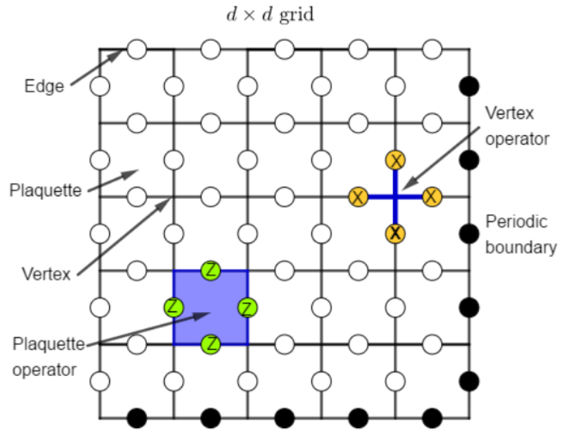
The toric code defined over an square lattice, consists of physical qubits placed on every edge of the lattice. The topology of the torus arises from two distinct boundary conditions, one for the left and right edge of the lattice and one for the top and bottom edges. The stabilizer group of the toric code is generated by two distinct stabilizers associated with the plaquettes and vertices of the lattice (see Fig. 1). Specifically, to every plaquette, , and vertex , the operators
| (4) |
are stabilizers of the toric code, and there are a total of independent plaquette and vertex operators forming the generators of its stabilizer group. Observe that adjacent plaquette and vertex operators commute as they overlap on exactly two physical qubits. Products of plaquette (vertex) operators are also stabilizers of the torus and give rise to trivial loops as illustrated in Fig. 1.

The dimension of the code space is . The logical operators, , for each of the logical qubits are shown in Fig. 2. They form non-trivial closed loops around the torus with forming horizontal loops, vertical loops and the corresponding being closed loops orthogonal to those of . Notice, however, that the construction of the logical operators is not unique: we can generate an equivalence class of logical operators, acting identically on the code space, by multiplying the above logical operators with elements of (i.e., the loops do not need to be straight).
From the preceding discussion it follows that for a logical error to occur, an odd number of non-trivial loops around the torus must occur. Therefore, the distance of the toric code is . If a physical qubit suffers an error, the stabilizer generators adjacent to the position of the physical qubit will have error syndrome . However, the error syndrome distribution is never one to one with the physical errors of the lattice. There can be many different combinations of physical errors which lead to the same error syndrome, as shown in Fig. 3. Therefore, smart strategies are needed to return the faulty state to the initial logical sate. The agent must perform physical operations which do not result in non-trivial loops around the torus, and thus logical errors, whilst returning the state to the codespace.


In addition, the design of optimal decoders also relies heavily on the types of errors occurring as well as their distribution. The simplest and most common noise models assume that each qubit experiences an independent and identically distributed (i.i.d.) noise process, with a probability of suffering an error. Among the uncorrelated noise models, the most relevant ones are bit-flip ( errors) and phase-flip ( errors) errors. For correlated errors, depolarizing noise ( noise each with probability ) is the most paradigmatic noise model. In this work we shall only consider uncorrelated noise and without loss of generality we shall assume bit-flip noise (analysis for phase-flip errors is completely analogous). Correlated noise is more challenging and will be addressed in future work. The optimal threshold of a decoder, on the other hand, is the maximum value of for which recovery of the information is possible. For the toric code under i.i.d bit-flip errors this threshold is known to be Dennis et al. 2002.
A widely used decoder for the toric code under bit-flip errors is based on the minimum weight perfect matchings (MWPM) algorithm Gabow 1976; Cook and Rohe 1999. MWPM adopts the policy of correcting for the most likely error given a particular error syndrome and has proven to be a very successful decoder with an estimated threshold of Browne 2014. Recently, machine learning techniques and applications of (deep) neural networks have been applied in search for optimal decoders, both for topological as well as standard QECC Varsamopoulos et al. 2017; Krastanov and Jiang 2017; Baireuther et al. 2018; Fösel et al. 2018; Chamberland and Ronagh 2018; Sweke et al. 2018; Liu and Poulin 2019; Varsamopoulos et al. 2019; Andreasson et al. 2019. We now review the main techniques in reinforcement learning which we will use in search of efficient decoders for the toric code.
III Reinforcement learning
Reinforcement learning (RL) is a framework within which one can precisely formulate the old dictum of “learning through experience” Sutton et al. 1998. Agents trained using RL have excelled at performing certain tasks, such as mastering the game of Go Silver et al. 2016, better than humans and RL based agents are used extensively in robotics Orr and Müller 2003, artificial intelligence Ramos et al. 2017, and face-recognition Brunelli and Poggio 1993. Here we introduce the agent-environment paradigm of RL and review its key features; state and state-action valued functions. We then briefly discuss deep Q-learning (DQL) which uses deep convolutional networks highlighting some key techniques used to guarantee convergence in the training process for the agent.
Consider a scenario involving an agent, , sequentially interacting with its immediate environment, , in order to learn how to achieve a specific task (see Fig. 4). Here, learning is to be understood as ’s ability to refine its future behaviour based on past experience in order to maximise future reward. Regardless of the details of , , and their interaction any such learning scenario can be modelled using the following three ingredients Sutton et al. 1998: the set of all possible states, , of , the set of all possible actions, , of , and the set of rewards, —an assessment of ’s performance towards the task. If the interaction is known, then one talks of model-based RL, otherwise the latter is model-free.
The learning process of can be described in terms of episodes 11 1 Note that we can always consider finite sequences by introducing a terminal state for the environment indicating that the task is completed.. and interact, as shown in Fig. 4, and the episode finishes when the agent reaches the terminal state. Any given step in an episode consists of receiving the reward —from her/his previous action—and the current state of , . then performs action , after which sends reward , and its state changes to . Here boldface subscripts for the actions and state changes to the state of the environment indicate that these may depend on the history of actions and past states of the environment.
The set of states, rewards, and actions of an episode are random variables, and the interaction between and is a stochastic map , that may depend on all preceding states of and actions of . Specifically, the probability that receives reward , and the state of at step is , given all preceding states and actions is . If the conditional probabilities depend solely on the last preceding state of and action of , i.e., then every finite sequence of steps is formally equivalent to a finite Markov decision process (MDP) Bellman 1957. The average reward an agent expects to obtain after performing action , given the state of the environment is , is then
| (5) |
Note that whilst we have assumed that both state and action spaces are finite dimensional, Eq. (5) can be equally applied to infinite dimensional cases.
The learning of the agent is quantified by the expected discounted return
| (6) |
where is the discount rate 22 2 The use of a discount rate is particularly useful for dealing with continuous interactions between agent and environment, i.e., for continuous sequences.; favours only immediate rewards, and for , larger values of give more importance to long-term rewards than smaller values of . In the limit, when , all rewards are given the same value. The decision making process of is known as a policy and consists of a complete specification of the actions will perform at every step of the sequence and for any possible state of . Given a state the probability that will perform action is denoted by . Under a policy the value of a state , , quantifies its average expected future returns., i.e., . Similarly, the value of an action given a state —known as the q-value — quantifies the average expected future returns of that action, i.e., . Such policy-value functions induce a partial order in the space of all possible policies of an agent: is at least as good as , if and only if . A policy is optimal if no other policy can give a higher value than it, Sutton et al. 1998.
To determine the optimal policy one makes use of the recursive nature of both , and to write
| (7) |
and
| (8) |
Eqs. (7), and (8) are known as the Bellman equations Bellman 1966 for state and state-action-value functions. For the optimal policy , takes the specific form
| (9) |
known as the Bellman optimality equation. Note that an optimal policy is known to always exist, though it may not be unique Puterman 2014.
Agent training: Deep Q-learning
If the environment in a MDP is known then the optimal policy can be obtained by solving Bellman equations. For model-free RL no such possibility exists and consequently state and state-action-value functions need to be estimated from experience. A typical algorithm used in this case is called Q-learning, with guaranteed convergence to the optimal -value if every state-action pair is observed a sufficiently large number of times, i.e., if the agent is trained infinitely long Sutton et al. 1998. For large state spaces this is prohibitively expensive. Consequently we have to resort to finite training sets which in turn means that the agent will often encounter situations previously unseen.
Deep Q-learning (DQL) uses deep convolutional networks Kalchbrenner et al. 2014, specialised for processing high-dimensional data, in order to extract global features and patterns. Upon encountering a previously unseen state, DQL uses such global features to compare with similar situations in past experience Mnih et al. 2015. DQL parametrises the -function in terms of a neural network, so that given an input state and action, the neural network produces the -value as an output. During training, the network parameters are adjusted, via stochastic gradient descent, such as to reduce the error between the optimal and approximated target -values.
We use DQL to train our agent to successfully decode uncorrelated bit or phase flip noise on the toric code. Training halts either after a certain number of episodes have happened, or until the loss function of the convolutional neural network stops decreasing. To ensure stability during training we also make use of additional training techniques, such as double deep Q-learning, duelling deep Q-learning, and prioritised experience replay Mnih et al. 2013; Simonini 2018.
IV Deep RL decoders for uncorrelated noise
We now cast decoders for the toric code under uncorrelated noise as a RL problem and present the results of training model-free agents to accomplish the task. As already mentioned we discuss only the case of bit-flip errors. The environment, , consists of the state of the toric code; a matrix of entries containing the position of errors applied to the physical qubits for any given episode. This state is hidden from and it is used to generate the state space , comprised of the error syndrome of all stabilisers of the code, in this case a set of matrices representing the position of each stabilizer and its corresponding error syndrome. This situation can be regarded as an example of a partially observable Markov decision process Barry et al. 2014.
The agents actions consist of single qubit bit flip operations. In principle, we can allow the agent to act on any of the qubits. However, it is inconvenient to let the agent perform bit-flip operations to qubits which do not have an adjacent violated syndrome. Such qubits are not candidates of having produced the syndrome errors, and thus should not be altered. Therefore, for a given state , i.e., a given error syndrome, only a subset of all possible actions (single qubit bit-flips) should be allowed and these actions are different for different syndrome errors. As the neural network needs to have a fixed output dimension, we need to make adjustments in order to appropriately accommodate the restrictions on the agents possible actions. One possibility would be to calculate the q-values for all qubits, and allow the agent to perform only the valid actions but this results in large training times for the agent. Whilst this strategy does work it is extremely inefficient, particularly for large lattice dimensions.
In order to speed up the learning stage, a convenient representation of the errors must given to the neural network. By exploiting the boundary conditions of the torus Andreasson et al. provide one such representation in terms of so-called perspectives shown in Fig. 5 Andreasson et al. 2019. The syndrome error of any stabilizer can be represented as an arbitrary plaquette at the center of the torus. For each syndrome we can generate a set of matrices—the perspectives –each of them having a different defect at its center while keeping the relative position of other defects fixed. The input to the neural network are the perspectives , for which the neural network provides the -value for each of the four possible actions; corrections on the qubits adjacent to the vertex in question. In other words, instead of inputing one single matrix containing the syndrome errors, matrices are given as an input, being the number of syndrome errors. In this way, the output of the neural network is reduced from to , allowing for a more efficient and stable training phase.

The agent continues to perform actions until the terminal state of the environment is reached: all syndrome measurements have outcome . As we compute the actions performs on the hidden state of the code along the way we can evaluate the number of non-trivial horizontal or vertical loops around the torus. If an even number of such loops is found, no logical errors have occurred and the agent is rewarded a nominal reward of 33 3 The value of the reward is chosen so as to speed-up the training process. Else, the agent’s reward is . In Andreasson et al. 2019, a RL decoder for the same task was designed using similar techniques as ours. There the agent was penalised with for every iteration, so that the optimal strategy would be to correct the error syndrome with the minimum number of operations. We shall refer to the decoder of Andreasson et al. 2019 as a minimum action decoder, or MAD for short, and will compare this reward scheme with ours.
We train the agent using the DQL algorithm, until the parameters of the convolutional neural network stabilize. In order to give the agent more freedom to explore the large policy space during training we use an -greedy strategy for -learning; with probability the agent selects the action with the highest value of the current -function, whereas with probability the agent performs an action at random. Furthermore, we vary the value of during training, linearly decreasing it to the minimum value of . Moreover, we also train the agent with an initially low probability of bit flip errors so that learns to correct properly, linearly increasing the occurrence of errors near-to and beyond the threshold of the code.
Neural Network architecture and training parameters
In this section we provide the technical details used to design the neural network and training phase of the agent. The neural network consists of some convolutional layers, a set of fully connected layers and an output layer with four values. Each output corresponds to applying an action to one of the qubits adjacent to the input plaquette. The algorithm we implement is given in Table 1. The network is trained by adjusting the hyper parameters at iteration such that the error between the optimal target values and the approximated target values , calculated using the Q-network, is reduced. Training consists in decreasing this loss function via stochastic gradient descend, until the Q-network produces precise values of the q-function.
The fact that the approximate target values depend on the network parameters produces instabilities in the training process, and could lead to divergence of the network weights. To that end we use a separate network for generating the targets in the Q-learning update. More precisely, for every updates we clone the active Q-network (the one used to select the best action in each state) to obtain a target Q-network, which is used to generate the targets for the following updates. Table 2 shows the parameters used for the neural network architecture. Table 2 shows the common hyper-parameters used for the agents, whilst table 3 shows the hyper-parameters which were different.
| With probability select a random action |
| Otherwise select action |
| Execute action , receive reward and next state |
| Store experience in memory |
| Select a random sample from D |
| Calculate target values , with if is a terminal state |
| Perform a gradient descent step on with respect to the network parameters : |
| Type | Size |
|---|---|
| Input layer | |
| Convolutional layer | 512 filters, size, stride |
| Convolutional layer | 256 filters, size, stride |
| Convolutional layer | 256 filters, size, stride |
| Fully-connected layer | 256 neurons |
| Fully-connected layer | 128 neurons |
| Fully-connected layer | 64 neurons |
| Fully-connected layer | 32 neurons |
| Output layer | 4 outputs |
| Parameter | Value | ||
|---|---|---|---|
| Input layer | |||
| Batch size | 32 | ||
| Maximum training steps | 1000 | ||
| Memory buffer size | 3000000 | ||
| Target update iterations | 500 | ||
| Learning rate | 0.0001 | ||
| 0.9 | |||
| 0.999 | |||
| Optimizer | Adam | ||
| Rewards |
|
| Agent | initial | final | iterations | initial | final | iterations with final | |
|---|---|---|---|---|---|---|---|
| 0.75 | 0.08 | 1000 | 0.01 | 0.10 | 300 | 0.9 | |
| 0.75 | 0.08 | 2500 | 0.01 | 0.10 | 1000 | 0.95 | |
| 0.75 | 0.08 | 6000 | 0.01 | 0.10 | 2000 | 0.95 | |
| 0.5 | 0.1 | 8000 | 0.01 | 0.10 | 3500 | 0.95 |
Results
We now present our results on RL decoders for uncorrelated noise on the toric code. Agents were trained on grids of dimensions, and . After training, we evaluated the decoders performance for different error probabilities . We define the logical success probability as the proportion of syndromes decoded successfully. As for uncorrelated errors the MWPM algorithm is near-optimal, we also compare the RL agent’s performance with MWPM.


Fig. 6 shows the logical success probability as a function of the error probability for several lattice sizes For the performance of the RL agent improves with the dimension , of the lattice. When the error probability is low, the probability of successful decoding increases with the dimension of the lattice, whereas for high the opposite effect occurs. The turning point between these two behaviors is called the code threshold. The code threshold for these agents falls between and , similar to those obtained in Andreasson et al. 2019. We also tested decoders which were trained with error probabilities higher than the code threshold . We noticed a slight increase in performance in the former case whilst in the latter decoders performed significantly worse.
A more direct comparison between our decoder and the one of Andreasson et al. 2019 is shown in Fig. 7. We trained an agent according to the reward system of Andreasson et al. 2019, and compared the episode length distribution for both agents.


For both agents seem to have very similar episode length distributions meaning that an agent trained based on success/failure reward learnt that, in general, the best strategy is indeed to nullify the error syndrome as quickly as possible even though it was not explicitly told so. For , the episode length distributions are more distinct. By and large the agent adopts a decoding strategy requiring the least amount of corrections but occasionally slightly more steps are required.
Our results indicate that it is not necessary to train agents based on minimizing their number of actions and that the natural choice of reward based on correct decoding is capable of learning the best policy, even yielding slight improvements in performance. A comparison of the efficiencies of the two decoders is shown in Fig. 8.


For both agents have very similar success probability. However, for , the agent trained with success/failure rewards outperforms the one of Andreasson et al. 2019 indicating that the different policy adopted by the success/failure agent is in fact beneficial for correct decoding of the code.
Finally, Table 4 shows the training times required for the various lattice sizes considered. All training was performed using a single desktop computer.
| Lattice dimension | d=3 | d=5 | d=7 | d=9 |
|---|---|---|---|---|
| Training time (hrs) | 0.33 | 5 | 12 | 32 |
V Summary and Conclusions
In this work we used deep Q-learning to train an agent using reinforcement learning in order to decode uncorrelated errors on a toric code. We showed that agents can be trained based on whether or not correct decoding of the errors has been performed and showed that such decoders achieve near optimal performance. Our agents are more versatile as compared to those trained based on minimising the number of actions taken, which leads to slightly improved performance on smaller lattices. Moreover, by comparing the episode length distributions between the two different types of agents we observe that indeed policies based on performing the minimum number of actions seem to form the most efficient decoders.
We believe that our model-free scheme of choosing rewards based solely on the success/failure of the decoding procedure is more versatile and can be used to design decoders for other TECC, such as surface codes, or the Kagome lattice, as well as for more general noise models. We expect that our approach is able to address error correction for correlated noise for which minimum action decoding methods are unsuitable. Work along this line is currently under consideration.
Acknowledgements
The authors acknowledge support from Spanish MINECO reference FIS2016-80681-P (with the support of AEI/FEDER,EU); the Generalitat de Catalunya, project CIRIT 2017-SGR-1127 and the Baidu-UAB collaborative project ’Learning of Quantum Hidden Markov Models’.
References
References
- Galindo and Martín-Delgado (2002) A. Galindo and M. A. Martín-Delgado, Rev. Mod. Phys. 74, 347 (2002).
- Georgescu et al. (2014) I. M. Georgescu, S. Ashhab, and F. Nori, Rev. Mod. Phys. 86, 153 (2014).
- Gisin and Thew (2007) N. Gisin and R. Thew, Nat. Photonics 1, 165 (2007).
- Giovannetti et al. (2011) V. Giovannetti, S. Lloyd, and L. Maccone, Nat. Photonics 5, 222 (2011).
- Degen et al. (2017) C. L. Degen, F. Reinhard, and P. Cappellaro, Rev. Mod. Phys. 89, 035002 (2017).
- Gottesman (2010) D. Gottesman, in Quantum information science and its contributions to mathematics, Proceedings of Symposia in Applied Mathematics, Vol. 68 (2010) pp. 13–58.
- Terhal (2015) B. M. Terhal, Rev. Mod. Phys. 87, 307 (2015).
- Campbell et al. (2017) E. T. Campbell, B. M. Terhal, and C. Vuillot, Nature 549, 172 (2017).
- Bravyi and Kitaev (1998) S. B. Bravyi and A. Kitaev, arXiv preprint quant-ph: 9811052 (1998).
- Bombín (2013) H. Bombín, arXiv preprint quant-ph: 1311.0277 (2013).
- Herold et al. (2015) M. Herold, E. T. Campbell, J. Eisert, and M. J. Kastoryano, npj Quantum information 1, 15010 (2015).
- Herold et al. (2017) M. Herold, M. J. Kastoryano, E. T. Campbell, and J. Eisert, New J. Phys. 19, 063012 (2017).
- Lang and Büchler (2018) N. Lang and H. P. Büchler, SciPost Phys. 4, 007 (2018).
- Kubica and Preskill (2019) A. Kubica and J. Preskill, Phys. Rev. Lett. 123, 020501 (2019).
- Duclos-Cianci and Poulin (2010a) G. Duclos-Cianci and D. Poulin, in 2010 IEEE Information Theory Workshop (IEEE, 2010) pp. 1–5.
- Duclos-Cianci and Poulin (2010b) G. Duclos-Cianci and D. Poulin, Phys. Rev. Lett. 104, 050504 (2010b).
- Torlai and Melko (2017) G. Torlai and R. G. Melko, Phys. Rev. Lett. 119, 030501 (2017).
- Varsamopoulos et al. (2017) S. Varsamopoulos, B. Criger, and K. Bertels, Quantum Science and Technology 3, 015004 (2017).
- Krastanov and Jiang (2017) S. Krastanov and L. Jiang, Sci Rep-UK 7, 11003 (2017).
- Baireuther et al. (2018) P. Baireuther, T. E. O’Brien, B. Tarasinski, and C. W. Beenakker, Quantum 2, 48 (2018).
- Fösel et al. (2018) T. Fösel, P. Tighineanu, T. Weiss, and F. Marquardt, Phys. Rev. X 8, 031084 (2018).
- Chamberland and Ronagh (2018) C. Chamberland and P. Ronagh, Quantum Science and Technology 3, 044002 (2018).
- Sweke et al. (2018) R. Sweke, M. S. Kesselring, E. P. van Nieuwenburg, and J. Eisert, arXiv preprint arXiv:1810.07207 (2018).
- Liu and Poulin (2019) Y.-H. Liu and D. Poulin, Phys. Rev. Lett. 122, 200501 (2019).
- Varsamopoulos et al. (2019) S. Varsamopoulos, K. Bertels, and C. G. Almudever, arXiv preprint arXiv:1901.10847 (2019).
- Maskara et al. (2019) N. Maskara, A. Kubica, and T. Jochym-O’Connor, Phys. Rev. A 99, 052351 (2019).
- Andreasson et al. (2019) P. Andreasson, J. Johansson, S. Liljestrand, and M. Granath, Quantum 3, 183 (2019).
- Edmonds (1965) J. Edmonds, Can. J. Math. 17, 449–467 (1965).
- Poulsen Nautrup et al. (2019) H. Poulsen Nautrup, N. Delfosse, V. Dunjko, H. J. Briegel, and N. Friis, Quantum 3, 215 (2019).
- Valenti et al. (2019) A. Valenti, E. van Nieuwenburg, S. Huber, and E. Greplova, Phys. Rev. Research 1, 033092 (2019).
- Lidar and Brun (2013) D. A. Lidar and T. A. Brun, Quantum error correction (Cambridge university press, 2013).
- Gottesman (1997) D. Gottesman, Stabilizer Codes and Quantum Error Correction, Ph.D. thesis, California Institute of Technology (1997).
- Poulin (2005) D. Poulin, Phys. Rev. Lett. 95, 230504 (2005).
- Yao et al. (2012) X.-C. Yao, T.-X. Wang, H.-Z. Chen, W.-B. Gao, A. G. Fowler, R. Raussendorf, Z.-B. Chen, N.-L. Liu, C.-Y. Lu, Y.-J. Deng, et al., Nature 482, 489 (2012).
- Nigg et al. (2014) D. Nigg, M. Mueller, E. A. Martinez, P. Schindler, M. Hennrich, T. Monz, M. A. Martin-Delgado, and R. Blatt, Science 345, 302 (2014).
- Hill et al. (2015) C. D. Hill, E. Peretz, S. J. Hile, M. G. House, M. Fuechsle, S. Rogge, M. Y. Simmons, and L. C. Hollenberg, Science Advances 1, e1500707 (2015).
- Córcoles et al. (2015) A. D. Córcoles, E. Magesan, S. J. Srinivasan, A. W. Cross, M. Steffen, J. M. Gambetta, and J. M. Chow, Nat. Commun. 6, 6979 (2015).
- Kelly et al. (2015) J. Kelly, R. Barends, A. G. Fowler, A. Megrant, E. Jeffrey, T. C. White, D. Sank, J. Y. Mutus, B. Campbell, Y. Chen, et al., Nature 519, 66 (2015).
- Riste et al. (2015) D. Riste, S. Poletto, M.-Z. Huang, A. Bruno, V. Vesterinen, O.-P. Saira, and L. DiCarlo, Nat. Commun. 6, 6983 (2015).
- Takita et al. (2016) M. Takita, A. D. Córcoles, E. Magesan, B. Abdo, M. Brink, A. Cross, J. M. Chow, and J. M. Gambetta, Phys. Rev. Lett. 117, 210505 (2016).
- Dennis et al. (2002) E. Dennis, A. Kitaev, A. Landahl, and J. Preskill, J. Math. Phys. 43, 4452 (2002).
- Gabow (1976) H. N. Gabow, JACM 23, 221 (1976).
- Cook and Rohe (1999) W. Cook and A. Rohe, INFORMS J. Comput. 11, 138 (1999).
- Browne (2014) D. Browne, “Lectures on topological codes and quantum computation,” (2014), (Accessed on 30/10/2019).
- Sutton et al. (1998) R. S. Sutton, A. G. Barto, et al., Introduction to reinforcement learning, Vol. 2 (MIT press Cambridge, 1998).
- Silver et al. (2016) D. Silver, A. Huang, C. J. Maddison, A. Guez, L. Sifre, G. Van Den Driessche, J. Schrittwieser, I. Antonoglou, V. Panneershelvam, M. Lanctot, et al., Nature 529, 484 (2016).
- Orr and Müller (2003) G. B. Orr and K.-R. Müller, Neural networks: tricks of the trade (Springer, 2003).
- Ramos et al. (2017) S. Ramos, S. Gehrig, P. Pinggera, U. Franke, and C. Rother, in 2017 IEEE Intelligent Vehicles Symposium (IV) (IEEE, 2017) pp. 1025–1032.
- Brunelli and Poggio (1993) R. Brunelli and T. Poggio, IEEE transactions on pattern analysis and machine intelligence 15, 1042 (1993).
- (50) Note that we can always consider finite sequences by introducing a terminal state for the environment indicating that the task is completed.
- Bellman (1957) R. Bellman, Indiana Univ. Math. J. 6, 679 (1957).
- (52) The use of a discount rate is particularly useful for dealing with continuous interactions between agent and environment, i.e., for continuous sequences.
- Bellman (1966) R. Bellman, Science 153, 34 (1966).
- Puterman (2014) M. L. Puterman, Markov decision processes: discrete stochastic dynamic programming (John Wiley & Sons, 2014).
- Kalchbrenner et al. (2014) N. Kalchbrenner, E. Grefenstette, and P. Blunsom, arXiv preprint arXiv:1404.2188 (2014).
- Mnih et al. (2015) V. Mnih, K. Kavukcuoglu, D. Silver, A. A. Rusu, J. Veness, M. G. Bellemare, A. Graves, M. Riedmiller, A. K. Fidjeland, G. Ostrovski, et al., Nature 518, 529 (2015).
- Mnih et al. (2013) V. Mnih, K. Kavukcuoglu, D. Silver, A. Graves, I. Antonoglou, D. Wierstra, and M. Riedmiller, arXiv preprint arXiv:1312.5602 (2013).
- Simonini (2018) T. Simonini, “Improvements in Deep Q Learning: Dueling Double DQN, Prioritized Experience Replay, and fixed Q-targets,” (2018).
- Barry et al. (2014) J. Barry, D. T. Barry, and S. Aaronson, Physical Review A 90, 032311 (2014).
- (60) The value of the reward is chosen so as to speed-up the training process.