fragmentation algorithm
Abstract
Collisional fragmentation is a ubiquitous phenomenon arising in a variety of astrophysical systems, from asteroid belts to debris and protoplanetary disks. Numerical studies of fragmentation typically rely on discretizing the size distribution of colliding objects into a large number of bins in mass space, usually logarithmically spaced. A standard approach for redistributing the debris produced in collisions into the corresponding mass bins results in calculation, which leads to significant computational overhead when is large. Here we formulate a more efficient explicit fragmentation algorithm, which works when the size spectrum of fragments produced in an individual collision has a self-similar shape with only a single characteristic mass scale (which can have arbitrary dependence on the energy and masses of colliding objects). Fragment size spectra used in existing fragmentation codes typically possess this property. We also show that our approach can be easily extended to work with non-self-similar fragment size distributions, for which we provide a worked example. This algorithm offers a substantial speedup of fragmentation calculations for large , even over the implicit methods, making it an attractive tool for studying collisionally evolving systems.
I. Introduction
The issue of collisional fragmentation regularly arises in astrophysical problems where the masses of colliding objects — e.g. planetesimals or dust particles in protoplanetary disks — need to be followed. Examples include evolution of the asteroid belt (Durda & Dermott 1997), the Kuiper Belt (Davis & Farinella 1997; Kenyon & Bromley 2004), dust populations in debris disks (Kenyon & Bromley 2005; Krivov et al. 2008), and protoplanetary disks (Brauer et al. 2008; Birnstiel et al. 2010). The large number of objects in these applications makes it convenient to characterize the state of the system via the mass distribution (spectrum) , such that the number of objects in the mass interval is . Pair-wise collisions cause mass to be exchanged between different parts of the mass space: a collision between objects and produces a number of fragments, channeling mass towards smaller objects. The total mass in the system of colliding objects is usually conserved in the process, although it may be lost in very energetic collisions when vaporization occurs; for simplicity we will disregard the latter possibility. Also, when particles reach very small sizes they could be removed from the system by other processes such as the Poynting-Robertson drag or radiation pressure.
In a continuous limit the evolution of the mass spectrum due to fragmentation in pair-wise collisions is described by the following equation:
| (1) | |||||
Here is the rate coefficient for collisions between particles of masses (target) and (projectile), while is the size (or mass) distribution of fragments produced in a single collision. It is defined such that the number of fragments in the mass interval resulting in a collision between particles and is . In numerical applications the mass coordinate is discretized into a large number of bins (typically uniformly spaced in ). The number of objects per -th bin is and the vector , fully characterizes the system. Equation (1) is then evolved in two steps. First, one chooses a pair of bins and , and computes the number of collisions between particles in these bins that occur in time . Second, the fragments produced in collisions of each mass pair are distributed over the bins according to their mass distribution (i.e. the function ), which is described by the first term on the right hand side of this equation. This procedure needs to be repeated for each pair of colliding bins.
The first step requires operations in general, while the second takes . As a result, the numerical cost of evolving equation (1) scales as per time step. This can be rather challenging when is very large, which is often needed to provide accurate description of collisional evolution of astrophysical systems spanning many orders of magnitude in mass.
The goal of this work is to demonstrate that the numerical cost can be reduced to for a certain class of fragment size distributions, which is rather common, and flexible enough to handle even more general models of collision outcomes. We describe this fragmentation model in §II and the associated algorithm in §III. We then show how this model can be extended to approximate more general forms of the fragment size distribution (§IV) and provide a numerical illustration in §V. We compare explicit and implicit methods for evolving fragmentation cascades in §VI. Our results are discussed in §VII.
II. Fragmentation model
The outcome of a collision between two objects depends on a variety of factors. The primary ones are the masses and involved in a collision, the relative velocity of the colliding objects , and the material properties of each object determined by the composition, structural characteristics (e.g. porosity) and size. The precise geometry of the collision (i.e. impact parameter for spherical objects) also plays an important role. In this study, to simplify the notation, we will keep track of the dependence of the collision outcome only on the masses of the colliding objects (in many studies the rates of the collisions and collision outcomes are treated in an averaged sense, by convolving over the distributions of , impact parameters, etc.).
We characterize the size distribution of fragments forming in a collision of objects with mass and using a reasonably general model of a collision outcome. It covers two most common possibilities, namely (1) the erosion in weakly energetic collisions, which results in one dominant post-collision remnant with the mass and a continuous spectrum of small fragments, and (2) catastrophic disruption, when the large remnant no longer exists and only a continuous spectrum of fragments remains. This model has a form
| (2) |
where in the case of erosion, while in the case of catastrophic collisions. Here is a mass spectrum describing a continuous population of fragments formed in a collision. There are other possible outcomes of particle collisions — sticking, mass transfer, bouncing, etc. (Güttler et al. 2010; Windmark et al. 2012) — which we do not consider in this study.
A particular form of explored in this work that allows one to reduce the computational cost of the fragmentation calculation to is the self-similar fragment mass spectrum
| (3) |
Here is an arbitrary function that truncates at large masses , is the characteristic mass scale set by , and the details of collision physics (i.e. collision energy), and is the normalization of the spectrum. As we will show later in §III, the key feature of this fragment mass spectrum is that all information about the collision details is absorbed in a single parameter — the mass scale .
The value of is set by mass conservation (in the absence of mass losses to vaporization)
| (4) |
so that
| (5) |
Integration over the mass coordinate can be to extended to infinity since the function vanishes for large values of .
Laboratory experiments suggest (Gault & Wedekind 1969; Hartmann 1969; Fujiwara et al. 1977; Blum & Münch 1993) that the fragment mass spectrum can often be described reasonably well by a power law in fragment mass truncated above some largest fragment mass :
For example, Fujiwara et al. 1977 found that the mass spectrum of fine fragments resulting in collisions of basaltic bodies can be well described by a power law dependence with index . On the other hand, Blum & Münch 1993 found that in their experiments with ZrCO4 aggregates. The spectrum (II) has the self-similar form (3) with
| (9) |
where and is the Heavyside step function.
III. fragmentation algorithm
We now demonstrate how the fragmentation calculation described by the equation (1) can be turned into an problem, rather than , for the fragment mass spectrum in the form (3). We will later show in §IV that this procedure can be generalized to cover even more complicated fragment mass spectra.
The basic idea behind this algorithm lies in the order in which different steps are performed. In the standard approach for every pair of mass bins the calculation of the collisional debris production is immediately followed by the redistribution step — assigning fragments to their corresponding mass bin. In our new method the order is different: after computing debris production for each mass bin pair we bin the outcomes (spectrum amplitudes ) according to their and , possible when has a self-similar shape (3). Only after this procedure has been carried out for all pairs of bins we perform the fragment distribution step. Both these steps, performed sequentially, can be computed in operations, providing the desired speedup. We next describe this algorithm in details.
Let us introduce two auxiliary -dimensional vectors. One is and is used to record the number of large remnant bodies resulting from erosive collisions in a fixed time interval that end up in the -th bin (i.e. with falling into this bin). Another vector is — the sum of normalization factors given by equation (5) for all collisions that have characteristic mass scale of their fragment size distributions falling into the -th mass bin.
We can now describe our fragmentation algorithm step by step.
- 1.
At the start of a new time step we set , , .
- 2.
We pick a particular mass bin , which is a operation.
- 3.
We first take care of the last term in the right hand side of equation (1); although, the order is not important. We consider collisions of objects in the -th bin with objects in every bins in the system, calculating their rate and the actual number of collisions in time :
(10) where , are the width of the -th and -th mass bin, respectively. Note that can be non-integer.
The total loss of particles from the -th bin is then
(11) Calculation of and for all combinations of and requires operations.
- 4.
We then deal with the first term in the right hand side of equation (1) and consider the spectrum of fragments resulting in collisions between objects in -th and -th bins considered before. Standard fragmentation algorithms directly distribute these fragments for each pair into the relevant mass bins already at this step (another operation). This would make the algorithm scale as .
We proceed differently. Knowing the relative energy of collision we compute the values of , and for every pair of and . We then treat large remnants and small debris as follows.
Large remnant bodies
We find the index of the bin into which falls, and increase the value of by the number of remnant bodies produced in collisions:(12) The factor is introduced here to conserve mass: it accounts for the fact that the large remnant mass does not necessarily equal the central mass of the bin .
Small fragments
We then take care of the continuous spectrum of smaller fragments. First, we determine the index of the bin into which falls. Since, again, in general , we ensure mass conservation by adjusting to a (slightly different) value , such that(13) This follows from the fact that the total mass of the self-similar fragment size spectrum with mass scale is , where is the integral defined in equation (5).
We then update the -th component of the vector as follows:
(14) - 5.
Operations in steps (2)-(4) are repeated for all pairs of and (avoiding double counting). This, in general, requires calculations, in the end of which vectors and get fully updated.
- 6.
Now we go through the final, redistribution, steps. We first update the number of objects in each bins as follows:
(15) where is the width of -th mass bin. In other words, we add to each bin all the large remnants and small fragments that originally fell within its corresponding mass interval. This step again uses operations.
Finally, contributions (sinks) from step (3) are subtracted for all bins:
(16) adding additional operations.
- 7.
Time is incremented by and steps (1)-(6) are repeated once again.
One can see that this algorithm indeed performs the fragmentation calculation using only operations per time step, and not as the conventional approach. This improvement can be achieved only when the collision outcome is described by the equation (3), with the mass spectrum of fragments being a self-similar function with a single characteristic mass scale .
Indeed, if depended on e.g. two mass scales, then the amplitude vector would need to be replaced with the 2-dimensional amplitude array. In that case the first part of the redistribution step (6) would have involved operations, since the summation in equation (15) would need to be carried out over two indices. Similarly, methods based on implicit time-integration are , see Section VI. Nevertheless, in the following sections we will show how algorithm can be applied also to some more general collision outcomes than the one given by the equation (3).
IV. Generalizations of the algorithm
The method presented in the previous section allows some straightforward generalizations that greatly extend its applicability. Such generalizations are possible when the spectrum of fragments can be represented or approximated using the self-similar components. We cover both cases below.
IV.1. Superposition of self-similar mass spectra
A rather straightforward extension of the algorithm outlined above is possible when the fragment mass spectrum can be represented as a sum of self-similar mass distributions:
| (17) |
where characteristic mass scales are distinct (i.e. not multiples of each other). In this case amplitudes can no longer be found from equation (5). Instead, they need to be specified independently, with the only constraint coming from the mass conservation:
| (18) | |||
| (19) |
For example, the full mass spectrum (2) can be viewed as a sum of two self-similar components: remnant spectrum with the amplitude and mass scale , and the continuous self-similar spectrum of small fragments given by the equation (3).
The only difference with the procedure described in §III is that instead of one amplitude vector we would introduce now such vectors and then repeat the steps (4)-(6) for all individual self-similar contributions. The number of operations would scale as .
IV.2. Piecewise approximation of the fragment spectrum
Our algorithm can also be used when the spectrum of the fragments can be approximated in a piecewise fashion using a number of self-similar components. For example, almost any fragment spectrum can be represented as a series of power law segments (within certain mass intervals) of the form
where is some average of within the interval . Fragment size distributions in the form of two (or more) broken power laws have been found in collisional experiments of Fujiwara et al. 1977, Takagi et al. 1984, Davis & Ryan 1990. But any reasonably smooth fragment mass spectrum can be approximated in this way given a sufficiently large number of components (mass intervals) .
Each of these components can be written as the difference of the two power law spectra defined by equation (II), namely
| (24) | |||||
Combining equations (IV.2) and (24) we see that ends up being approximated as a linear combination of self-similar (power law) components, which reduces the problem to the one already considered in §IV.1.
Note that one does not have to approximate as the sum of only power law segments ; other representations are possible too, as will be shown next.
V. Example calculation: piecewise approximation of the fragment spectrum

To demonstrate the accuracy and speedup associated with using our algorithm, we now provide an example of applying it to treat collisional evolution with a non-self-similar fragment size distribution. We consider a fragment mass spectrum
| (25) | |||||
with normalization , two mass scales, and , and two power law slopes and . This mass spectrum is exponentially truncated above . It behaves as a power law for , however, the power law slope smoothly changes to for very small fragments, .
Very importantly, is not a constant but changes as the collision characteristics (e.g. masses and ) vary. This makes given by equation (25) non-self-similar, which is illustrated in Figure 1. There we show how the shape of (multiplied by ) evolves as and vary, implying lack of self-similarity. Each of the curves is normalized such that the total mass in fragments is always (although in this figure we set for simplicity).


We can approximate the mass spectrum (25) as a superposition of three self-similar components as follows:
| (26) |
each of them featuring only one mass scale. This decomposition is illustrated in Figure 2. The first term (green dotted curve) is an exponentially truncated power law extending all the way down to very small fragment sizes; it is designed to fit the original spectrum (25) for . The second term (blue dashed line) is a power law with the same slope as in the first term, sharply truncated above . Its amplitude is chosen so that it fully offsets the first term below (note that it enters with the negative sign). Finally, the last component (dashed magenta line) is another power law sharply truncated at with the slope and amplitude chosen such that this term matches the behavior of the spectrum (25) for .
We now carry out two fragmentation calculations. One uses fragment mass spectrum (25) without approximations; because of its non-self-similar shape this calculation employs the standard fragmentation algorithm. The second calculation uses an approximation (26), allowing us to use our algorithm as described in §IV.2. Both of them use explicit time stepping (see Section VI for comparison with implicit calculations). In both cases, we evolve the system using Euler’s method. The time-step is chosen so that the number of particles in one bin will not change by more than 10 % in any one time-step (with an allowance for bins with a small number of particles in them). We then compare the outcomes of the two calculations, as well as the numerical costs involved.
In both cases we assume that is given by
| (27) |
where . We also choose
| (28) |
so that when goes down (e.g. for more energetic collisions), there is a larger range in , for which (i.e. more small fragments get formed). We use and in this calculation. At time all mass in the system is in objects with the same mass (monodisperse initial condition) occupying a single mass bin. The mass interval that we cover extends from to ; fragments falling below the lower mass end get removed from the system. We assume for simplicity that collisions lead to fragmentation only if . Also, we assume that no largest remnant remains, i.e. only the continuous spectrum of small fragments results in a fragmentation event. The collision rate is proportional to the geometric cross-section of the two colliding bodies, assuming all objects to be spheres of the same density. This setup is similar to that in Dohnanyi 1969 and Tanaka et al. 1996, except for the non-self-similar shape of the fragment spectrum.
Results of the two calculations are shown in Figure 3. There we plot the mass distributions (multiplied by and normalized to the initial mass and particle number) at different times during the calculation, for the two different algorithms run with different numbers of mass bins. Time, labelled on the panels, is in terms of the initial timescale for collisions between bodies in the initial mass bin. The height of the bin at shows the current number of particles in the initial mass bin normalized to the initial number of objects in the system.
We first discuss the general features of the collisional evolution in this calculation. Early on, at , the mass spectrum closely mirrors that of the assumed fragment size distribution (25). This is to be expected, since at that time the number of objects with is small enough (total mass in this part of the spectrum is ) for their mutual collisions to be rare. On the other hand, collisions between these fragment and the numerous large objects do occur, which explains a bump11 1 According to equation (27), collisions with smaller fragments result in larger . Because of our assumption of no fragmentation when , the largest possible is . This explains the gap between the initial mass bin at and the continuous spectrum of fragments, which persists at all times. appearing above . This bump becomes more pronounced at and fully morphs with the continuous mass spectrum by .
By the shape of the distribution of fragments starts to evolve away from the single-collision spectrum (25) at small . And by the fragment mass distribution attains a steady-state form, which can be viewed as a power law with superimposed wavy structure. The slope of this power law is close to 1/6 (shown in black in the bottom right panel), in agreement with the results of Dohnanyi 1969 and Tanaka et al. 1996. The wiggles on top of this power law are caused by the boundary condition at the low mass end, see Campo Bagatin et al. 1994 for a discussion of this effect. Beyond only the normalization of the size distribution changes, steadily decaying in time because of mass lost to particles smaller than our smallest mass bin, while its overall shape stays the same. The height of the bin goes down too. It drops by two orders of magnitude by , signaling substantial erosion of the initial population of objects.
V.1. Comparison of the and algorithms
We now compare the performance of the algorithm and the full calculation. We first note that for small numbers of bins (), there are substantial differences between the results of the two calculations at all times. However, as the number of bins increases, the results converge, with two algorithms agreeing with each other quite well already for . Minor differences remain, especially at early times (when there is still a strong sensitivity to the shape of the input fragment spectrum), as even in the limit of an infinite number of bins, the fragment mass distributions are slightly different near (see Figure 2). This can be seen, for example, near (right around for collisions of two objects) at for . Nevertheless, at late times these differences get largely wiped out. Thus, we can conclude that already with 5-10 mass bins per decade our algorithm is able to reproduce the fine details of the collisional evolution even for non-self-similar fragment size spectrum.
Turning now to the computational cost of each algorithm, in Figure 4 we show the wall clock time to run them as a function of the number of bins . We use an adaptive time-step, so the number of time-steps required to evolve the distribution for a given simulation time is slightly different between the two algorithms, and for different numbers of bins. For that reason, we plot both the amount of time required to reach a fixed simulation time (, upper panel), and the time required to execute 400 steps of the run (lower panel).
There are slight variations in the run time even for the exact same parameters, presumably caused by the evolving state of the computing hardware. For this reason, for each algorithm and number of bins, we run the calculation 10 times, hence the multiple points shown in Figure 4 for each number of bins. We then calculate the best fit lines through the points for each algorithm, assuming and scalings, correspondingly. These are the solid lines in the figure. We also calculate the best fit lines without fixing their slopes, which are shown as the dotted lines. These slopes turn out to be 2.04 and 2.98 in the top panel, and 1.96 and 2.90 in the bottom panel, in good agreement with the theoretical expectations.
VI. Implicit Versus Explicit Time Stepping
A number of studies have used implicit time integration methods to evolve the coagulation-fragmentation equations (Brauer et al. 2008; Birnstiel et al. 2010; Garaud et al. 2013; Booth et al. 2018). The advantage of these methods has traditionally been that they allow much longer time steps to be used in the integration, leading to a faster time to solution despite the increased complexity of the method. However, these studies did not make use of the fragmentation algorithm, which can only be used with explicit time stepping.
The difference between explicit and implicit methods can be summarized as follows. Master equation (1) written in a discretized form in mass space has a form of a system of equations
| (29) |
where, as before, and vector stands for the expressions in the right hand side of equation (1) written out for each . When evolving this system, explicit updates by in time take the form
| (30) |
whereas implicit updates reduce to solving the system of equations
| (31) |
for . Writing , the solution can be found via Newton-Raphson iteration, in which the estimate is updated via
| (32) |
where is the identity matrix.
The appearance of the Jacobian, , and matrix inversion in the above equation prevents implicit methods from benefiting from the computation of the fragmentation rate because both the Jacobian computation and the matrix inversion in equation (32) require operations to compute. The complexity of the Jacobian calculation can be understood from equation (14) as is an matrix.
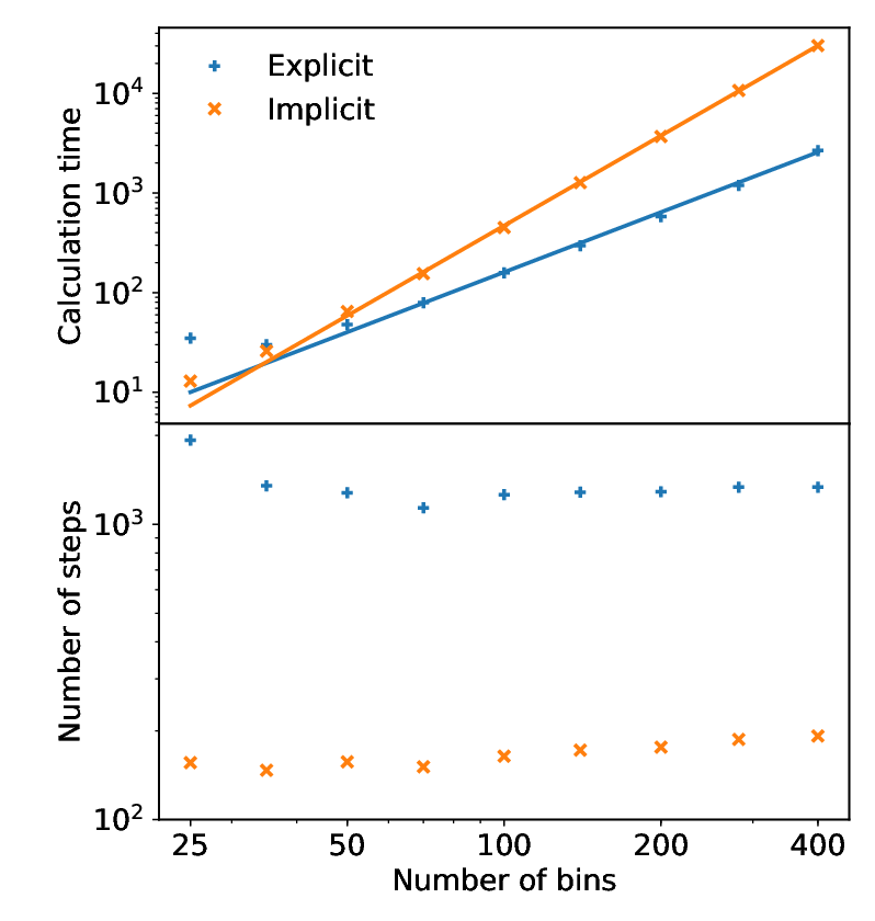
To compare the efficiency of implicit and explicit schemes, we use a simplified version of the problem presented in section V.1. We take the fragment spectrum to have a self-similar form
| (33) |
with defined by equation (27) as before. In this case, to integrate these equations we choose two 3rd-order methods, the explicit 3rd-order Runge-Kutta method of Gottlieb & Shu 1998 and the implicit 3rd-order Rosenbrock method of Rang & Angermann 2005 used by Booth et al. 2018. Both of these methods provide an embedded error estimates, which are used to adapt the time step to ensure that the relative error is below 1 per cent. For the implicit scheme we use the traditional fragmentation algorithm while the scheme is used with the explicit time integration scheme.
The time taken and number of steps required by the schemes to integrate the fragmentation equations to in units of initial collisional timescales are shown in Fig. 5. While the implicit method requires a factor 7 – 9 fewer steps than the explicit scheme (bottom panel), the extra cost of the algorithm outweighs this for problems with more than about 50 cells (top panel). Tests on problems including both coagulation and fragmentation lead to similar conclusions.
VII. Discussion
The main result of this work is the algorithm for numerical treatment of fragmentation in collisional systems, described in §III. The main condition necessary for this approach to work is that the continuous size distribution of fragments resulting in an individual collision depends on a single mass scale . This algorithm is insensitive to the details of the actual dependence of the different characteristics of the fragment mass spectrum — , , and , see equations (2)-(3) — on the energy and masses of objects involved in a collision.
Self-similarity of is not a highly demanding requirement since the majority of numerical studies of fragmentation in astrophysical systems use such self-similar size distributions of fragments anyway, typically in the form of a truncated power law (II), see Greenberg et al. 1978, Kenyon & Luu 1999, Löhne et al. 2008, Brauer et al. 2008, Birnstiel et al. 2010. On the other hand, implementation of this algorithm allows substantial gains in computational efficiency, significantly reducing the time consumed by fragmentation simulations with large number of mass bins, , see §V.1.
Moreover, as we showed in §IV-V, the algorithm can be applied even when the fragment size spectrum is not a simple self-similar function with a single mass scale; one just need to approximate the non-self-similar fragment size distribution using several self-similar components. A practical example shown in §V demonstrates that the differences between a calculation carried with this algorithm and the direct ‘exact’ calculation, which takes much longer, are very minor (at the level of several per cent or less) in systems that have evolved for longer than their characteristic collisional timescale. At early times the level of agreement is dictated mainly by the accuracy with which the original complicated spectrum of fragments is approximated by the self-similar components.
There is a reason why approximating even rather complicated non-self-similar fragment size distributions (e.g. measured in some experiments, Fujiwara et al. 1977) with a simple self-similar shape works in practice. The characteristics of the steady-state collisional cascades are known to be rather insensitive to the input fragment size spectrum . For example, Tanaka et al. 1996 has shown that as long as is self-similar with , the slope of the steady-state cascade should be sensitive only to the scaling of the collision rate with the masses of objects involved in a collision, but not to the actual form of . Similarly, O’Brien & Greenberg 2003 have shown that the slope of the collisional cascade depends on the mass scaling of the energy necessary to disrupt an object, but not on the power law of the fragment size spectrum (as long as ). By abandoning the assumption , Belyaev & Rafikov 2011 were able to demonstrate the sensitivity of the steady-state cascade to the shape of the fragment size spectrum; however, the variation was found to be very weak (logarithmic). This is one of the reasons why on long time intervals, after several collisional timescales have passed and the system settled into a steady-state cascade, our algorithm performs just as well as the exact calculation, see Figure 3c,d.
Fragmentation algorithms documented in the literature (e.g. Greenberg et al. 1978; Kenyon & Luu 1999; Löhne et al. 2008; Brauer et al. 2008; Windmark et al. 2012; Garaud et al. 2013, etc.) redistribute the debris produced in collisions in the direct manner as described in §I and are thus . To the best of our knowledge, Booth et al. 2018 is the only other study mentioning the possibility of constructing algorithm for self-similar fragment size distributions, however, without providing details. Our present study is intended partly to fill this gap.
A number of studies invoke implicit time integration (Brauer et al. 2008; Birnstiel et al. 2010; Garaud et al. 2013), which has an complexity due to the Jacobian calculation. The benefit of these schemes has traditionally been that the larger time steps they allow outweigh the additional cost in solving the linear system, which is only a factor when already using an fragmentation algorithm. Since our algorithm is about an order of magnitude faster than an implicit method per step already for , this means that the time-step for implicit methods must be smaller by a similar factor to remain competitive. Although Brauer et al. 2008 did achieve a reduction in the number of time steps by a factor by using implicit methods for a problem including both grain growth and radial drift, this was primarily because radial drift limits the time-step in the explicit code to smaller values than those required by coagulation/fragmentation calculation. Without computing radial drift implicitly, the explicit approach is substantially faster, as demonstrated in Fig. 5. The simplicity of our algorithm also makes it easier to implement and parallelize, as well as using less memory than fully implicit methods (as the entire Jacobian need not be stored). This makes our algorithm more attractive for complex problems.
Recently, simulations of dust dynamics in protoplanetary disks started including evolution of the dust size distribution due to coagulation/fragmentation spatially resolved in multiple dimensions (Li et al. 2019; Drazkowska et al. 2019). As this is done using the existing framework of Birnstiel et al. 2010, there is an associated computational overhead that scales steeply with the number of mass bins used to characterize dust size distribution. Use of our fragmentation algorithm would substantially reduce the computational cost of such calculations, making this tool an attractive option for future (multi-dimensional) studies of the dust evolution in disks around young stars.
References
- Belyaev & Rafikov (2011) Belyaev, M. A., & Rafikov, R. R. 2011, Icarus, 214, 179
- Birnstiel et al. (2010) Birnstiel, T., Dullemond, C. P., & Brauer, F. 2010, A&A, 513, A79
- Blum & Münch (1993) Blum, J., & Münch, M. 1993, Icarus, 106, 151
- Booth et al. (2018) Booth, R. A., Meru, F., Lee, M. H., & Clarke, C. J. 2018, MNRAS, 475, 167
- Brauer et al. (2008) Brauer, F., Dullemond, C. P., & Henning, T. 2008, A&A, 480, 859
- Campo Bagatin et al. (1994) Campo Bagatin, A., Cellino, A., Davis, D. R., Farinella, P., & Paolicchi, P. 1994, Planet. Space Sci., 42, 1079
- Davis & Farinella (1997) Davis, D. R., & Farinella, P. 1997, Icarus, 125, 50
- Davis & Ryan (1990) Davis, D. R., & Ryan, E. V. 1990, Icarus, 83, 156
- Dohnanyi (1969) Dohnanyi, J. S. 1969, J. Geophys. Res., 74, 2531
- Drazkowska et al. (2019) Drazkowska, J., Li, S., Birnstiel, T., Stammler, S. M., & Li, H. 2019, arXiv e-prints, arXiv:1909.10526
- Durda & Dermott (1997) Durda, D. D., & Dermott, S. F. 1997, Icarus, 130, 140
- Fujiwara et al. (1977) Fujiwara, A., Kamimoto, G., & Tsukamoto, A. 1977, Icarus, 31, 277
- Garaud et al. (2013) Garaud, P., Meru, F., Galvagni, M., & Olczak, C. 2013, ApJ, 764, 146
- Gault & Wedekind (1969) Gault, D. E., & Wedekind, J. A. 1969, J. Geophys. Res., 74, 6780
- Gottlieb & Shu (1998) Gottlieb, S., & Shu, C. W. 1998, Mathematics of Computation, 67, 73
- Greenberg et al. (1978) Greenberg, R., Wacker, J. F., Hartmann, W. K., & Chapman, C. R. 1978, Icarus, 35, 1
- Güttler et al. (2010) Güttler, C., Blum, J., Zsom, A., Ormel, C. W., & Dullemond, C. P. 2010, A&A, 513, A56
- Hartmann (1969) Hartmann, W. K. 1969, Icarus, 10, 201
- Kenyon & Bromley (2004) Kenyon, S. J., & Bromley, B. C. 2004, AJ, 128, 1916
- Kenyon & Bromley (2005) —. 2005, AJ, 130, 269
- Kenyon & Luu (1999) Kenyon, S. J., & Luu, J. X. 1999, AJ, 118, 1101
- Krivov et al. (2008) Krivov, A. V., Müller, S., Löhne, T., & Mutschke, H. 2008, ApJ, 687, 608
- Li et al. (2019) Li, Y.-P., Li, H., Ricci, L., et al. 2019, ApJ, 878, 39
- Löhne et al. (2008) Löhne, T., Krivov, A. V., & Rodmann, J. 2008, ApJ, 673, 1123
- O’Brien & Greenberg (2003) O’Brien, D. P., & Greenberg, R. 2003, Icarus, 164, 334
- Rang & Angermann (2005) Rang, J., & Angermann, L. 2005, BIT Numerical Mathematics, 45, 761
- Takagi et al. (1984) Takagi, Y., Mizutani, H., & Kawakami, S.-I. 1984, Icarus, 59, 462
- Tanaka et al. (1996) Tanaka, H., Inaba, S., & Nakazawa, K. 1996, Icarus, 123, 450
- Windmark et al. (2012) Windmark, F., Birnstiel, T., Güttler, C., et al. 2012, A&A, 540, A73