跳到论文正文
W Papers独立论文阅读器 arXiv:1911.01859 论文正文 计算阅读时间 · 0%
引用这篇论文根据当前论文元数据生成,正式投稿前建议核对。


License: arXiv.org perpetual non-exclusive license
arXiv:1911.01859v2 [stat.ME] 28 Feb 2020

The correlation-assisted missing data estimator

Timothy I. Cannings    Yingying Fan Affiliation: University of Edinburgh and University of Southern California
Abstract

We introduce a novel approach to estimation problems in settings with missing data. Our proposal – the Correlation-Assisted Missing data (CAM) estimator – works by exploiting the relationship between the observations with missing features and those without missing features in order to obtain improved prediction accuracy. In particular, our theoretical results elucidate general conditions under which the proposed CAM estimator has lower mean squared error than the widely used complete-case approach in a range of estimation problems. We showcase in detail how the CAM estimator can be applied to UU-Statistics to obtain an unbiased, asymptotically Gaussian estimator that has lower variance than the complete-case UU-Statistic. Further, in nonparametric density estimation and regression problems, we construct our CAM estimator using kernel functions, and show it has lower asymptotic mean squared error than the corresponding complete-case kernel estimator. We also include practical demonstrations throughout the paper using simulated data and the Terneuzen birth cohort and Brandsma datasets available from CRAN.

Keywords: Missing data, UU-Statistics, kernel density estimation, local constant regression, nonparametric

1 Introduction

Data is a primary commodity in today’s economy, it is valued and traded like any other asset. Statistics and machine learning allow us to extract this value by improving operational efficiency, increasing revenue, or understanding the behaviour of customers. A common complication in modern applications is that the data may be incomplete. For example, some users may choose not to disclose their personal details (age, gender, geographic location, etc.) to a smartphone application; optional questions on an on-line form are often left blank; or data is sometimes removed or hidden to guarantee privacy. In other situations, missing data problems can arise when two or more different data sources have been combined.

Missing data is not a new problem. As early as the 1950s, Anderson 1957 found the maximum likelihood estimator in a multivariate normal distribution when some of the observations were missing. In a seminal paper, Rubin 1976 studied missing data in a rigorous general framework, introduced the notion of data missing at random, and specified conditions under which the process that causes data to be missing may be ignored. See also the comprehensive book on the subject by Little and Rubin 2002 and the recent special issue of Statistical Science (Josse and Reiter 2018).

A simple and widely used approach to deal with missing data is to discard any incomplete observations – a technique referred to as complete-case analysis (Little and Rubin 2002, Chapter 3). There is an obvious drawback with this method that perhaps much of the data is ignored. An alternative approach is to impute the missing values (Ford 1983). There is an extensive body of work on different imputation techniques; see, for instance, Little and Rubin 2002 and Molenberghs et al. 2015 for an overview. Other techniques are based on the expectation–maximisation (EM) algorithm (Dempster et al. 1977). Missing data has also been studied in a range of high-dimensional settings, including regression (Loh and Wainwright 2012), classification (Cai and Zhang 2018), and (sparse) principal component analysis (Elsener and van de Geer 2018; Zhu et al. 2019).

In this paper, we develop a novel approach to missing data problems. Our new proposal, the correlation-assisted missing data (CAM) estimator, exploits the relationship between the complete cases and the observations with missing values, in order to improve on the performance of the complete-case estimator. More precisely, we construct an (approximately) mean-zero statistic, using both the complete-cases and the data with missing entries, which is correlated with the complete-case estimator. We then exploit this correlation to construct our new estimator, by making a linear adjustment to the complete-case estimator.

Our first main result, Proposition 1, elucidates when the proposed CAM estimator will be more accurate than the complete-case estimator in terms of mean squared error. The result does not require any assumptions on the data generating mechanism. In particular, we do not assume the data to be missing completely at random. Further, Proposition 1 motivates an optimal (but typically unknown) choice of the adjustment term used in the construction of the CAM estimator. This optimal choices leads to the greatest reduction in mean squared error. We also show that we can then construct a data-driven version of the CAM estimator that performs well in many practical settings.

As a second main contribution, we showcase how the CAM estimation technique can be applied in specific settings. First, when the complete-case estimator is a U-Statistic, we show that the optimal adjustment term also takes the form of a U-statistic. This motivates us to consider a CAM estimator with a general U-statistic as the adjustment term and allows for detailed theoretical analysis. In particular, when the data is missing completely at random, we show that our CAM estimator is unbiased, asymptotically Gaussian, and has a smaller asymptotic variance than the complete-case UU-Statistic (cf. Theorem 3). We provide two concrete examples where a clear improvement can be shown analytically. Moreover, the numerical properties of the CAM estimator are demonstrated using simulated and real data, including an application using the Terneuzen birth cohort dataset available from CRAN.

We then investigate an application of the CAM technique to kernel based methods in nonparametric density estimation and regression problems. Under standard nonparametric assumptions on the data generating distribution, we quantify the leading order asymptotic improvement in mean squared error obtained by the CAM estimator compared with the complete-case approach. We provide further theoretical justification for the construction of the CAM estimator in these settings, in terms of approximating the optimal adjustment term. This leads to a fast, fully data-driven construction of our estimator. Finally, we demonstrate our method and the improvement it offers over the compete-case estimator in a simulation study and show how it can be used in an application with the Brandsma dataset on CRAN.

Related methods to the CAM approach have been utilised in various double-sample design settings. Fuller 1998 considers the problem of marginal mean estimation when one observes a small set of pairs of data and a larger set of univariate observations. Chen and Chen 2000 proposed an estimator of the regression parameters in a generalised linear model, where the practitioner has one sample in which the observations may be noisy or proxy versions of the variables of interest, and a second validation sample where complete and exact observations of the features are available. Chen and Chen 2000 show that their estimator of the regression parameter is asymptotically unbiased and has smaller (asymptotic) variance than a naive estimator based solely on the validation sample. Similar ideas have been used more recently in different statistical problems. Jiang et al. 2011 propose a nonparametric kernel-based regression estimate in double sampling designs, where the response is missing in one of the samples, but a surrogate outcome is observed instead. Yang and Ding 2019 propose an estimator of the average causal treatment effect in a general setting, by combining multiple observational datasets; see also Lin and Chen 2014, who focus on the logistic regression setting. Very recently, Zhang et al. 2019 considered estimating the marginal mean response in a semi-supervised setting, where one has a large number of unlabelled observations alongside a small labelled training dataset. Our work extends these existing works to a much wider range of estimation problems, including UU-Statistics and nonparametric density estimation and regression.

Finally, we note here that, in contrast to many imputation approaches, the CAM technique has a clear and direct aim – that is to reduce the mean squared error of the complete-case estimator. On the other hand, while imputation is widely applicable, the properties of estimators derived from imputed data are typically not well understood. Indeed, imputation methods are often treated as a black-box solution to missing data problems, and the subsequent steps of estimation and inference are conducted independently of the imputation step, which may lead to unreliable results. In our numerical work in Section 4.3, we see that a regression estimator computed with imputed data can in fact perform worse than simply using a complete-case approach. Moreover, in problems such as density estimation, it is unclear whether imputation offers a viable solution – the distribution of the imputed data may not be the same as the target distribution.

The remainder of this paper is as follows. In Section 2 we fix our general statistical and missing data settings and introduce the CAM estimator. Section 3 is dedicated to studying UU-Statistics. We then demonstrate how the CAM estimator can be applied using kernel methods in density estimation and regression problems in Section 4. We also provide, throughout the paper, a number of practical demonstrations of the method using real and simulated datasets. We conclude our paper with a discussion of various practical considerations and possible extensions in Section 5. All technical details and proofs of our theoretical results are presented in Section A in the Appendix. We first end this section with an illustrative example that demonstrates how our estimator is constructed.

1.1 Illustrative example

Let (X1,Y1)T,…,(X2​n,Y2​n)T(X_{1},Y_{1})^{T},\ldots,(X_{2n},Y_{2n})^{T} be independent and identically distributed N2​(ν,Γ)N_{2}(\nu,\Gamma) variables, where ν=(νX,νY)T∈ℝ2\nu=(\nu_{X},\nu_{Y})^{T}\in\mathbb{R}^{2} is unknown but the covariance Γ=(Γi​j)\Gamma=(\Gamma_{ij}) is known. Suppose we observe {(X1,Y1),…,(Xn,Yn)}\{(X_{1},Y_{1}),\ldots,(X_{n},Y_{n})\} and {Yn+1,…,Y2​n}\{Y_{n+1},\ldots,Y_{2n}\}; in other words, in the language of missing data, the first component is missing completely at random in the second set of observations. Our task is to estimate νX\nu_{X}.

Refer to caption
Refer to caption
Figure 1: Left: 500 observations from the joint distribution of (U,V)(U,V) (see (1)), with νX=νY=1\nu_{X}=\nu_{Y}=1, Γ=110​I+910​(1,1)T​(1,1)\Gamma=\frac{1}{10}I+\frac{9}{10}(1,1)^{T}(1,1) and n=1000n=1000. Right: Sampling distributions of ν^X,1\hat{\nu}_{X,1} in black and ν~X\tilde{\nu}_{X} in red.

The complete-case estimator in this example ignores the second set of observations and takes the sample mean of the XX observations only. That is ν^X,1:=1n​∑i=1nXi∼N⁡(νX,Γ11/n)\hat{\nu}_{X,1}:=\frac{1}{n}\sum_{i=1}^{n}X_{i}\sim N(\nu_{X},\Gamma_{11}/n); this is unbiased and is the maximum likelihood estimator if there are no YY observations. Now consider ν^Y,1:=1n​∑i=1nYi\hat{\nu}_{Y,1}:=\frac{1}{n}\sum_{i=1}^{n}Y_{i} and ν^Y,2:=1n​∑i=n+12​nYi\hat{\nu}_{Y,2}:=\frac{1}{n}\sum_{i=n+1}^{2n}Y_{i}. Then, letting U:=ν^X,1U:=\hat{\nu}_{X,1} and V:=ν^Y,1−ν^Y,2V:=\hat{\nu}_{Y,1}-\hat{\nu}_{Y,2}, we have

(U,V)T∼N2​((νX,0)T,Γ~),(U,V)^{T}\sim N_{2}((\nu_{X},0)^{T},\tilde{\Gamma}), (1)

where Γ~=n−1​Γ+n−1​Γ22​(0,1)T​(0,1)\tilde{\Gamma}=n^{-1}\Gamma+n^{-1}\Gamma_{22}(0,1)^{T}(0,1); see Figure 1. This motivates the estimator

ν~X:=ν^X,1−Γ~12Γ~22​(ν^Y,1−ν^Y,2)∼N⁡(νX,1n​(Γ11−Γ~122Γ~22)).\tilde{\nu}_{X}:=\hat{\nu}_{X,1}-\frac{\tilde{\Gamma}_{12}}{\tilde{\Gamma}_{22}}(\hat{\nu}_{Y,1}-\hat{\nu}_{Y,2})\sim N\Bigl(\nu_{X},\frac{1}{n}\Bigl(\Gamma_{11}-\frac{\tilde{\Gamma}_{12}^{2}}{\tilde{\Gamma}_{22}}\Bigr)\Bigr). (2)

We see that ν~X\tilde{\nu}_{X} is also unbiased for νX\nu_{X}, but has a strictly smaller variance than ν^X,1\hat{\nu}_{X,1} whenever Γ12≠0\Gamma_{12}\neq 0.

There is a neat connection between our estimator and the Rao–Blackwell Theorem in this example. The statistic T=(T1,T2)T=(ν^X,1−ν^Y,1​Γ12/Γ22,ν^Y,1+ν^Y,2)TT=(T_{1},T_{2})^{T}=(\hat{\nu}_{X,1}-\hat{\nu}_{Y,1}\Gamma_{12}/\Gamma_{22},\hat{\nu}_{Y,1}+\hat{\nu}_{Y,2})^{T} is sufficient (the technical details are presented in Section A.1) for ν\nu, and the Rao–Blackwellised version of ν^X,1\hat{\nu}_{X,1} is 𝔼⁡(ν^X,1|T)=ν~X\mathbb{E}(\hat{\nu}_{X,1}|T)=\tilde{\nu}_{X}. In fact, one can show that ν~X\tilde{\nu}_{X} is the maximum likelihood estimator of νX\nu_{X} in this setting (cf. Anderson 1957).

2 Missing data and the CAM estimator

Suppose Z=(X,Y)Z=(X,Y) is a random pair taking values in ℝd×ℝ\mathbb{R}^{d}\times\mathbb{R} with joint distribution PP. We are interested in estimating some function of this distribution, θ=θ⁡(P)∈ℝ\theta=\theta(P)\in\mathbb{R}, say. Examples studied in detail in this paper include the mean of the first component of XX; the covariance between XX and YY; the value of a regression function of YY on XX at the point x∈ℝdx\in\mathbb{R}^{d}; or the value of the density fX​(x)f_{X}(x), if it exists, of XX at x∈ℝdx\in\mathbb{R}^{d}.

We study a setting where some of the features of XX are missing, but where the response YY is always observed. In order to model this, suppose that we have (Z,M)(Z,M), where the marginal distribution of ZZ is PP, and MM is a missingness indicator taking values in {0,1}d\{0,1\}^{d}. More precisely, we only observe the features j∈{1,…,d}j\in\{1,\ldots,d\}, with Mj=0M^{j}=0, that is ZM:=(XM,Y)Z^{M}:=(X^{M},Y), where for x=(x1,…,xd)T∈ℝdx=(x^{1},\ldots,x^{d})^{T}\in\mathbb{R}^{d} and m=(m1,…,md)T∈{0,1}dm=(m^{1},\ldots,m^{d})^{T}\in\{0,1\}^{d}, we write xm:=(xj:mj=0)∈ℝdmx^{m}:=(x^{j}:m^{j}=0)\in\mathbb{R}^{d_{m}}, where dm:=∑j=1d𝟙{mj=0}d_{m}:=\sum_{j=1}^{d}\mathbbm{1}_{\{m^{j}=0\}}. Define the missingness probabilities pm​(x,y):=ℙ⁡(M=m|X=x,Y=y)p_{m}(x,y):=\mathbb{P}(M=m|X=x,Y=y). Further write PmP_{m} and QmQ_{m} for the joint distribution of (Xm,Y)(X^{m},Y) and (Xm,Y)|{M=m}(X^{m},Y)|\{M=m\}, respectively. Note that under certain missing data assumptions we have Pm=QmP_{m}=Q_{m}, but that this is not the case in general.

We say the data is missing completely at random (MCAR) if MM is independent of the pair (X,Y)(X,Y). In this case we write pm:=ℙ⁡(M=m)p_{m}:=\mathbb{P}(M=m). The data is missing at random (MAR) if the missingness indicator only depends on the observed data. Formally, this means that MM is conditionally independent of ZZ given ZMZ^{M}. Whereas, the data is said to be missing not at random (MNAR) if MM depends on the unobserved value. See, for example, Little and Rubin 2002 for further discussion of these three scenarios. Our most general results in this paper make no assumption on the missingness type. For our technical analysis in the UU-Statistics and nonparametric learning problems, we focus on the MCAR case. Further discussion of the more challenging non-MCAR scenarios is given in Section 5.

Let (Z1,M1),…,(Zn,Mn)(Z_{1},M_{1}),\ldots,(Z_{n},M_{n}) be independent and identically distributed pairs with the same distribution as (Z,M)(Z,M). We observe Z1M1,…,ZnMnZ_{1}^{M_{1}},\ldots,Z_{n}^{M_{n}}. The popular complete-case approach uses only the observations with Mi=(0,…,0)∈ℝdM_{i}=(0,\ldots,0)\in\mathbb{R}^{d}. Our goal in this paper is to construct an estimator which also uses the observations with missing values in order to improve on the performance of the complete-case estimator.

It is convenient to consider the missingness indicators M1,…,MnM_{1},\ldots,M_{n} as fixed and equal to m1,…,mnm_{1},\ldots,m_{n}, and from this point on all probability statements should be interpreted to be conditional on (M1,…,Mn)=(m1,…,mn)(M_{1},\ldots,M_{n})=(m_{1},\ldots,m_{n}). It is also useful to introduce some further notation here. For m∈{0,1}dm\in\{0,1\}^{d}, let Am:={i∈{1,…,n}:mi=m}A_{m}:=\{i\in\{1,\ldots,n\}:m_{i}=m\} be the set of indices of the data missing mm, let nm:=|Am|n_{m}:=|A_{m}|. In particular, A0A_{0} is the set of indices of the complete cases, where here and throughout we use the shorthand 00 in place of 0d:=(0,…,0)∈ℝd0_{d}:=(0,\ldots,0)\in\mathbb{R}^{d}. We have that Am1∩Am2=∅A_{m_{1}}\cap A_{m_{2}}=\emptyset for m1≠m2m_{1}\neq m_{2}. Finally, for a set A⊆{1,…,n}A\subseteq\{1,\ldots,n\} and m∈{0,1}dm\in\{0,1\}^{d}, let 𝒯A,m:={Zim:i∈A}\mathcal{T}_{A,m}:=\{Z^{m}_{i}:i\in A\}. Of course, 𝒯A,m\mathcal{T}_{A,m} is not necessarily observed for every AA and mm, but we do observe 𝒯Am,m\mathcal{T}_{A_{m},m}. We assume that A0A_{0} is non-empty, and moreover, for each m∈{0,1}dm\in\{0,1\}^{d} with AmA_{m} non-empty, we have that limn→∞nmn=qm∈(0,1)\lim_{n\rightarrow\infty}\frac{n_{m}}{n}=q_{m}\in(0,1), almost surely. That is, either a set of features mm is never missing, or, for those that are missing, the relative sample sizes are more or less balanced. If the data is MCAR, then we have that qm=pmq_{m}=p_{m}, for m∈{0,1}dm\in\{0,1\}^{d}.

We now define a generic version of our correlation-assisted missing data (CAM) estimator. The main idea underpinning our proposal is to mimic the approach in the toy example in Section 1.1 by combining appropriate, correlated estimators, which are constructed using different parts of the data. We first assume that there is a suitable complete-case estimator of θ\theta that only uses the data in 𝒯A0,0\mathcal{T}_{A_{0},0}; this is denoted by θ^0=θ^A0,0\hat{\theta}_{0}=\hat{\theta}_{A_{0},0}. Furthermore, suppose that, for each mm and each A⊆{1,…,n}A\subseteq\{1,\ldots,n\}, we have access to a statistic denoted by θ^A,m\hat{\theta}_{A,m}, which only depends on the data in 𝒯A,m\mathcal{T}_{A,m}. Notice that, for m≠0m\neq 0, θ^A,m\hat{\theta}_{A,m} is not an estimator for θ\theta. A detailed discussion of the choice of θ^A,m\hat{\theta}_{A,m} is given at the end of this section.

Consider m∈{0,1}d∖{0d}m\in\{0,1\}^{d}\setminus\{0_{d}\} such that AmA_{m} is non-empty. The CAM estimator is constructed using θ^0\hat{\theta}_{0}, θ^Am,m\hat{\theta}_{A_{m},m} and θ^A0,m\hat{\theta}_{A_{0},m}. The hope is that the latter two statistics have similar expected values, and that θ^A0,m\hat{\theta}_{A_{0},m} is (highly) correlated with the complete-case estimator θ^0\hat{\theta}_{0}. We then exploit this correlation in the same way as we did in the illustrative example – see (2).

In fact, we can construct similar statistics using many m∈{0,1}d∖{0d}m\in\{0,1\}^{d}\setminus\{0_{d}\} simultaneously. Let ℳ⊆{0,1}d∖{0d}\mathcal{M}\subseteq\{0,1\}^{d}\setminus\{0_{d}\} denote the set of values of mm that we would like to use (a detailed discussion of how to choose ℳ\mathcal{M} in practice is postponed until Section 5). Consider the two column vectors of length |ℳ||\mathcal{M}|, given by θ^0,ℳ:=({θ^A0,m:m∈ℳ})T\hat{\theta}_{0,\mathcal{M}}:=\bigl(\{\hat{\theta}_{A_{0},m}:m\in\mathcal{M}\}\bigr)^{T} and θ^ℳ:=({θ^Am,m:m∈ℳ})T\hat{\theta}_{\mathcal{M}}:=\bigl(\{\hat{\theta}_{A_{m},m}:m\in\mathcal{M}\}\bigr)^{T}. Finally, for γ∈ℝ|ℳ|\gamma\in\mathbb{R}^{|\mathcal{M}|}, define the correlation-assisted missing data (CAM) estimator

θ^γℳ:=θ^0−γT​(θ^0,ℳ−θ^ℳ).\hat{\theta}_{\gamma}^{\mathcal{M}}:=\hat{\theta}_{0}-\gamma^{T}(\hat{\theta}_{0,\mathcal{M}}-\hat{\theta}_{\mathcal{M}}).

In practice we will use a data-driven choice of γ\gamma, which aims to minimise the mean squared error (cf. the discussion after the statement of Proposition 1).

We now study properties of the CAM approach in the general estimation problem. For an estimator θ^\hat{\theta}, let MSE⁡(θ^)=𝔼⁡{(θ^−θ)2}\mathrm{MSE}(\hat{\theta})=\mathbb{E}\{(\hat{\theta}-\theta)^{2}\} denote its mean squared error. Let b⁡(θ^):=𝔼⁡(θ^−θ)b(\hat{\theta}):=\mathbb{E}(\hat{\theta}-\theta) be the bias of an estimator θ^\hat{\theta} and let Bℳ:=𝔼⁡(θ^0,ℳ−θ^ℳ)B_{\mathcal{M}}:=\mathbb{E}(\hat{\theta}_{0,\mathcal{M}}-\hat{\theta}_{\mathcal{M}}). Let Ω\Omega denote the |ℳ||\mathcal{M}|-dimensional vector of covariances Cov⁡(θ^0,θ^0,ℳ)\mathrm{Cov}(\hat{\theta}_{0},\hat{\theta}_{0,\mathcal{M}}) and let Λ\Lambda be the |ℳ|×|ℳ||\mathcal{M}|\times|\mathcal{M}| covariance matrix Var⁡(θ^0,ℳ−θ^ℳ)\mathrm{Var}(\hat{\theta}_{0,\mathcal{M}}-\hat{\theta}_{\mathcal{M}}).

Proposition 1.

We have that

MSE⁡(θ^γℳ)−MSE⁡(θ^0)=γT​(Λ+Bℳ​BℳT)​γ−2​γT​{Ω+b⁡(θ^0)​Bℳ}.\displaystyle\mathrm{MSE}(\hat{\theta}_{\gamma}^{\mathcal{M}})-\mathrm{MSE}(\hat{\theta}_{0})=\gamma^{T}(\Lambda+B_{\mathcal{M}}B_{\mathcal{M}}^{T})\gamma-2\gamma^{T}\{\Omega+b(\hat{\theta}_{0})B_{\mathcal{M}}\}.

In particular, if Λ\Lambda is nonsingular and Bℳ=0B_{\mathcal{M}}=0, then γ=γ∗:=Λ−1​Ω\gamma=\gamma^{*}:=\Lambda^{-1}\Omega is the optimal weight vector achieving the maximum reduction in MSE, and

MSE⁡(θ^γ∗ℳ)−MSE⁡(θ^0)=−ΩT​Λ−1​Ω≤0.\mathrm{MSE}(\hat{\theta}_{\gamma^{*}}^{\mathcal{M}})-\mathrm{MSE}(\hat{\theta}_{0})=-\Omega^{T}\Lambda^{-1}\Omega\leq 0.

Proposition 1 compares the MSE of our CAM estimator and the complete-case estimator. We have made no assumption on the missing data mechanism and, in particular, we do not assume here that the data is missing completely at random. It is worth noting, however, that if the data is not MCAR, the complete-case estimator may be (even asymptotically) biased (cf. Section 5). In which case, simply improving on the performance of the complete-case estimator will not necessarily be effective. Furthermore, for general missing data mechanisms, we do not have control of BℳB_{\mathcal{M}}. However, we will see that under appropriate conditions in many estimation problems, θ^0,ℳ−θ^ℳ\hat{\theta}_{0,\mathcal{M}}-\hat{\theta}_{\mathcal{M}} will be (asymptotically) mean zero.

We see from the second part of Proposition 1 that to achieve maximum mean squared error reduction when Bℳ=0B_{\mathcal{M}}=0, we should set γ=γ∗:=Λ−1​Ω\gamma=\gamma^{*}:=\Lambda^{-1}\Omega. If, moreover, ℳ={m}\mathcal{M}=\{m\}, then we have that

MSE⁡(θ^γ∗ℳ)−MSE⁡(θ^0)=−Var⁡(θ^0)​Var⁡(θ^0,m)Var⁡(θ^0,m)+Var⁡(θ^m)​Corr2​(θ^0,θ^0,m).\mathrm{MSE}(\hat{\theta}_{\gamma^{*}}^{\mathcal{M}})-\mathrm{MSE}(\hat{\theta}_{0})=-\mathrm{Var}(\hat{\theta}_{0})\frac{\mathrm{Var}(\hat{\theta}_{0,m})}{\mathrm{Var}(\hat{\theta}_{0,m})+\mathrm{Var}(\hat{\theta}_{m})}\text{Corr}^{2}(\hat{\theta}_{0},\hat{\theta}_{0,m}).

Here we have used that θ^0,m\hat{\theta}_{0,m} and θ^m\hat{\theta}_{m} are independent since there are constructed using disjoint sets of observations. Thus, to achieve a maximal reduction in MSE, we’d like θ^0,m\hat{\theta}_{0,m} to be maximally correlated with θ^0\hat{\theta}_{0} and Var⁡(θ^m)\mathrm{Var}(\hat{\theta}_{m}) to be minimised. The first is achieved by the conditional expectation θ^0,m∗=𝔼⁡(θ^0|𝒯A0,m)\hat{\theta}_{0,m}^{*}=\mathbb{E}(\hat{\theta}_{0}|\mathcal{T}_{A_{0},m}). Moreover, Var⁡(θ^m)\mathrm{Var}(\hat{\theta}_{m}) is minimised by θ^m∗=𝔼⁡(θ^0,m)\hat{\theta}_{m}^{*}=\mathbb{E}(\hat{\theta}_{0,m}), but this is typically unknown. In practice, we use the data 𝒯Am,m\mathcal{T}_{A_{m},m} to construct an estimate of 𝔼⁡(θ^0,m)\mathbb{E}(\hat{\theta}_{0,m}) that has low variance. The situation when |ℳ|>1|\mathcal{M}|>1 is similar by noting the independence of 𝒯Am1,m1\mathcal{T}_{A_{m_{1}},m_{1}} and 𝒯Am2,m2\mathcal{T}_{A_{m_{2}},m_{2}}, for m1≠m2m_{1}\neq m_{2}.

To understand this further, note that with the optimal choice θ^0,m∗\hat{\theta}_{0,m}^{*} we have

Cov⁡(θ^0,θ^0,m∗)=𝔼⁡{Cov⁡(θ^0,θ^0,m∗|𝒯A0,m)}+Cov⁡{𝔼⁡(θ^0|𝒯A0,m),𝔼⁡(θ^0,m∗|𝒯A0,m)}=Var⁡(θ^0,m∗).\mathrm{Cov}(\hat{\theta}_{0},\hat{\theta}^{*}_{0,m})=\mathbb{E}\{\mathrm{Cov}(\hat{\theta}_{0},\hat{\theta}^{*}_{0,m}|\mathcal{T}_{A_{0},m})\}+\mathrm{Cov}\{\mathbb{E}(\hat{\theta}_{0}|\mathcal{T}_{A_{0},m}),\mathbb{E}(\hat{\theta}^{*}_{0,m}|\mathcal{T}_{A_{0},m})\}=\mathrm{Var}(\hat{\theta}^{*}_{0,m}).

Thus, in the ideal case that Var⁡(θ^m)\mathrm{Var}(\hat{\theta}_{m}) is negligible compared with Var⁡(θ^0,m∗)\mathrm{Var}(\hat{\theta}^{*}_{0,m}) (e.g. if nm≫n0n_{m}\gg n_{0}), the improvement in MSE is simply Var⁡(θ^0,m∗)=Var⁡{𝔼⁡(θ^0|𝒯A0,m)}\mathrm{Var}(\hat{\theta}^{*}_{0,m})=\mathrm{Var}\{\mathbb{E}(\hat{\theta}_{0}|\mathcal{T}_{A_{0},m})\}.

Of course, the conditional expectation 𝔼⁡(θ^0|𝒯A0,m)\mathbb{E}(\hat{\theta}_{0}|\mathcal{T}_{A_{0},m}) is also typically unknown. We will see in practice that, for instance, assuming a parametric form for θ^0,m∗\hat{\theta}_{0,m}^{*} works well. In particular, in our study of UU-Statistics in Section 3, we see that a data-driven choice of θ^0,m\hat{\theta}_{0,m} will often lead to similar performance to the optimal choice. Moreover, for nonparametric methods using kernels, the optimal θ^0,m∗\hat{\theta}_{0,m}^{*} can often be well approximated by the same type of nonparametric estimator with a practical choice of kernel (see Section 4).

3 UU-Statistics

In this section we specialise to the setting of UU-Statistics. Suppose we are interested in estimating a parameter of the form θ=θ⁡(P)=𝔼⁡{ϕ⁡(Z1,…,Zr)}\theta=\theta(P)=\mathbb{E}\bigl\{\phi\bigl(Z_{1},\ldots,Z_{r}\bigr)\bigr\}, for r≥1r\geq 1 and some function ϕ:(ℝd×ℝ)⊗r→ℝ\phi:(\mathbb{R}^{d}\times\mathbb{R})^{\otimes{r}}\rightarrow\mathbb{R}, which is permutation symmetric in its rr arguments. In the non-missing setting, an unbiased estimator of θ\theta is given by

θ^=1(nr)​∑{i1,…,ir}⊆{1,…,n}ϕ⁡(Zi1,…,Zir),\hat{\theta}=\frac{1}{{n\choose r}}\sum_{\{i_{1},\ldots,i_{r}\}\subseteq\{1,\ldots,n\}}\phi\bigl(Z_{i_{1}},\ldots,Z_{i_{r}}\bigr),

where the sum is taken over all unordered subsets {i1,…,ir}⊆{1,…,n}\{i_{1},\ldots,i_{r}\}\subseteq\{1,\ldots,n\} of size rr. Statistics of this form have been studied in detail in the non-missing setting, see for instance van der Vaart 1998. In particular, if 𝔼⁡{ϕ2​(Z1,…,Zr)}<∞\mathbb{E}\bigl\{\phi^{2}\bigl(Z_{1},\ldots,Z_{r}\bigr)\bigr\}<\infty, then n1/2(θ^−θ)→dN(0,r2ψU)n^{1/2}(\hat{\theta}-\theta)\rightarrow^{d}N(0,r^{2}\psi_{U}), where ψU=Cov⁡{ϕ⁡(Z1,…,Zr),ϕ⁡(Z1,Zr+1,…,Z2​r−1)}.\psi_{U}=\mathrm{Cov}\{\phi\bigl(Z_{1},\ldots,Z_{r}\bigr),\phi\bigl(Z_{1},Z_{r+1},\ldots,Z_{2r-1}\bigr)\}.

We now construct the CAM UU-Statistic. First, the complete-case UU-Statistic is

θ^0=θ^A0,0=1(n0r)​∑{i1,…,ir}⊆A0ϕ⁡(Zi1,…,Zir),\hat{\theta}_{0}=\hat{\theta}_{A_{0},0}=\frac{1}{{n_{0}\choose r}}\sum_{\{i_{1},\ldots,i_{r}\}\subseteq A_{0}}\phi\bigl(Z_{i_{1}},\ldots,Z_{i_{r}}\bigr),

where now the sum is taken over all unordered subsets {i1,…,ir}⊆A0\{i_{1},\ldots,i_{r}\}\subseteq A_{0} of size rr. In this case, for m∈ℳm\in\mathcal{M}, we have

𝔼(θ^0|𝒯A0,m)=1(n0r)∑{i1,…,ir}⊆A0𝔼{ϕ(Zi1,…,Zir)|Zi1m,…,Zirm}.\mathbb{E}(\hat{\theta}_{0}|\mathcal{T}_{A_{0},m})=\frac{1}{{n_{0}\choose r}}\sum_{\{i_{1},\ldots,i_{r}\}\subseteq A_{0}}\mathbb{E}\{\phi\bigl(Z_{i_{1}},\ldots,Z_{i_{r}}\bigr)|Z_{i_{1}}^{m},\ldots,Z_{i_{r}}^{m}\}.

In other words, the optimal form of the adjustment term in the construction of the CAM estimator is itself a UU-Statistic with kernel 𝔼{ϕ(Z1,…,Zr)|Z1m,…,Zrm}\mathbb{E}\{\phi\bigl(Z_{1},\ldots,Z_{r}\bigr)|Z_{1}^{m},\ldots,Z_{r}^{m}\}. This depends on ϕ\phi and the conditional distribution of ZZ given ZmZ^{m}, which is typically unknown. We therefore consider a general construction of the adjustment term as follows: for m∈ℳm\in\mathcal{M}, let ϕm:(ℝdm×ℝ)⊗r→ℝ\phi_{m}:(\mathbb{R}^{d_{m}}\times\mathbb{R})^{\otimes{r}}\rightarrow\mathbb{R} be a permutation symmetric function in its rr arguments, and, for A⊆{1,…,n}A\subseteq\{1,\ldots,n\}, define

θ^A,m=1(|A|r)​∑{i1,…,ir}⊆Aϕm​(Zi1m,…,Zirm).\hat{\theta}_{A,m}=\frac{1}{{|A|\choose r}}\sum_{\{i_{1},\ldots,i_{r}\}\subseteq A}\phi_{m}\bigl(Z_{i_{1}}^{m},\ldots,Z_{i_{r}}^{m}\bigr).

We will make use of θ^0,m=θ^A0,m\hat{\theta}_{0,m}=\hat{\theta}_{A_{0},m} and θ^m=θ^Am,m\hat{\theta}_{m}=\hat{\theta}_{A_{m},m}. Recall that θ^0,ℳ=(θ^0,m:m∈ℳ)T\hat{\theta}_{0,\mathcal{M}}=(\hat{\theta}_{0,m}:m\in\mathcal{M})^{T} and θ^ℳ=(θ^m:m∈ℳ)T\hat{\theta}_{\mathcal{M}}=(\hat{\theta}_{m}:m\in\mathcal{M})^{T}. For γ∈ℝ|ℳ|\gamma\in\mathbb{R}^{|\mathcal{M}|}, define the CAM UU-Statistic

θ^γℳ:=θ^0−γT​(θ^0,ℳ−θ^ℳ).\hat{\theta}_{\gamma}^{\mathcal{M}}:=\hat{\theta}_{0}-\gamma^{T}(\hat{\theta}_{0,\mathcal{M}}-\hat{\theta}_{\mathcal{M}}).

Here ϕm\phi_{m} is left unspecified, in practice one would aim to choose ϕm\phi_{m} to mimic to optimal choice above. In fact, we show in Theorem 2 that the CAM UU-Statistic has smaller mean squared error than the complete-case UU-Statistic whenever Cov⁡{ϕ⁡(Z1,…,Zr),ϕm​(Z1m,Zr+1m,…,Z2​r−1m)}≠0\mathrm{Cov}\{\phi\bigl(Z_{1},\ldots,Z_{r}\bigr),\phi_{m}\bigl(Z_{1}^{m},Z_{r+1}^{m},\ldots,Z_{2r-1}^{m}\bigr)\}\neq 0.

Suppose that the data is missing completely at random. Then we have that Bℳ=𝔼⁡(θ^0,ℳ−θ^ℳ)=0B_{\mathcal{M}}=\mathbb{E}(\hat{\theta}_{0,\mathcal{M}}-\hat{\theta}_{\mathcal{M}})=0. Recall also that Ω=Cov⁡(θ^0,θ^0,ℳ)\Omega=\mathrm{Cov}(\hat{\theta}_{0},\hat{\theta}_{0,\mathcal{M}}) and Λ=Var⁡(θ^0,ℳ−θ^ℳ)\Lambda=\mathrm{Var}(\hat{\theta}_{0,\mathcal{M}}-\hat{\theta}_{\mathcal{M}}). It follows directly from Proposition 1 that MSE⁡(θ^γℳ)−MSE⁡(θ^0)=γT​Λ​γ−2​γT​Ω.\mathrm{MSE}(\hat{\theta}_{\gamma}^{\mathcal{M}})-\mathrm{MSE}(\hat{\theta}_{0})=\gamma^{T}\Lambda\gamma-2\gamma^{T}\Omega.

Our next two results concern the asymptotic properties of the CAM UU-Statistic. Let ΩU\Omega_{U} be the |ℳ||\mathcal{M}|-dimensional vector with entries

ΩU,m:=Cov⁡{ϕ⁡(Z1,…,Zr),ϕm​(Z1m,Zr+1m,…,Z2​r−1m)}.\Omega_{U,m}:=\mathrm{Cov}\bigl\{\phi\bigl(Z_{1},\ldots,Z_{r}\bigr),\phi_{m}\bigl(Z_{1}^{m},Z_{r+1}^{m},\ldots,Z_{2r-1}^{m}\bigr)\bigr\}.

Further, let ΛU\Lambda_{U} be the |ℳ|×|ℳ||\mathcal{M}|\times|\mathcal{M}| symmetric matrix with diagonal entries

ΛU,m,m:=(1+p0pm)​Cov​{ϕm​(Z1m,…,Zrm),ϕm​(Z1m,Zr+1m,…,Z2​r−1m)}\Lambda_{U,m,m}:=\Bigl(1+\frac{p_{0}}{p_{m}}\Bigr)\mathrm{Cov}\bigl\{\phi_{m}\bigl(Z_{1}^{m},\ldots,Z_{r}^{m}\bigr),\phi_{m}\bigl(Z_{1}^{m},Z_{r+1}^{m},\ldots,Z_{2r-1}^{m}\bigr)\bigr\}

and off-diagonal entries

ΛU,m1,m2:=Cov⁡{ϕm1​(Z1m1,…,Zrm1),ϕm2​(Z1m2,Zr+1m2,…,Z2​r−1m2)}.\Lambda_{U,m_{1},m_{2}}:=\mathrm{Cov}\bigl\{\phi_{m_{1}}\bigl(Z_{1}^{m_{1}},\ldots,Z_{r}^{m_{1}}\bigr),\phi_{m_{2}}\bigl(Z_{1}^{m_{2}},Z_{r+1}^{m_{2}},\ldots,Z_{2r-1}^{m_{2}}\bigr)\bigr\}.

We see in Theorem 2 that, under moment assumptions, we have Ω→ΩU\Omega\rightarrow\Omega_{U} and Λ→ΛU\Lambda\rightarrow\Lambda_{U} as n→∞n\rightarrow\infty, and that the CAM UU-Statistic is unbiased and asymptotically Gaussian.

Theorem 2.

Suppose the data is missing completely at random, 𝔼⁡{ϕ2​(Z1,…,Zr)}<∞\mathbb{E}\{\phi^{2}\bigl(Z_{1},\ldots,Z_{r}\bigr)\}<\infty and, for m∈ℳm\in\mathcal{M}, 𝔼⁡{ϕm2​(Z1m,…,Zrm)}<∞\mathbb{E}\{\phi_{m}^{2}\bigl(Z_{1}^{m},\ldots,Z_{r}^{m}\bigr)\}<\infty. Then, for γ∈ℝ|ℳ|\gamma\in\mathbb{R}^{|\mathcal{M}|},

n0(θ^γℳ−θ)→dN(0,r2(ψU+γTΛUγ−2γTΩU))\sqrt{n_{0}}(\hat{\theta}_{\gamma}^{\mathcal{M}}-\theta)\rightarrow^{d}N\bigl(0,r^{2}(\psi_{U}+\gamma^{T}\Lambda_{U}\gamma-2\gamma^{T}\Omega_{U})\bigr)

as n→∞n\rightarrow\infty.

Theorem 2 shows that an asymptotically optimal choice of γ\gamma, which minimises the asymptotic variance of the CAM UU-Statistic, is γ∗=ΛU−1​ΩU\gamma^{*}=\Lambda_{U}^{-1}\Omega_{U}. The optimal leading order asymptotic variance reduction is n0−1​r2​ΩUT​ΛU−1​ΩUn_{0}^{-1}r^{2}\Omega_{U}^{T}\Lambda_{U}^{-1}\Omega_{U}. This is of the same order as the asymptotic variance of the complete-case UU-Statistic, which is n0−1​r2​ψUn_{0}^{-1}r^{2}\psi_{U}. Of course ΩU\Omega_{U} and ΛU\Lambda_{U} are typically unknown. However, to estimate these we can further exploit the use of UU-Statistics. Note that

ΩU,m\displaystyle\Omega_{U,m} =12𝔼[{ϕ(Z1,…,Zr)−ϕ(Z2​r,…,Z3​r−1)}\displaystyle=\frac{1}{2}\mathbb{E}\bigl[\bigl\{\phi(Z_{1},\ldots,Z_{r})-\phi(Z_{2r},\ldots,Z_{3r-1})\bigr\}
{ϕm(Z1m,Zr+1m,…,Z2​r−1m)−ϕm(Z2​rm,Z3​rm,…,Z4​r−2m)}].\displaystyle\hskip 150.0pt\bigl\{\phi_{m}(Z^{m}_{1},Z^{m}_{r+1},\ldots,Z^{m}_{2r-1})-\phi_{m}(Z_{2r}^{m},Z_{3r}^{m},\ldots,Z_{4r-2}^{m})\bigr\}\bigr].

Thus, we can estimate ΩU\Omega_{U} using a UU-Statistic of order 4​r−24r-2 (see (A.3) in Section A.3). A similar expression can be derived for the entries of ΛU\Lambda_{U}, but for brevity we exclude the formulas here – they are given in (A.3) and (A.3) in Section A.3. Let Λ^U\hat{\Lambda}_{U} and Ω^U\hat{\Omega}_{U} denote resulting UU-Statistic estimators of ΛU\Lambda_{U} and ΩU\Omega_{U}, respectively. (In practice, averaging over all subsamples of size 4​r−24r-2 will be computationally expensive, in our simulations Ω^U\hat{\Omega}_{U} and Λ^U\hat{\Lambda}_{U} are approximated using 10510^{5} random subsamples.)

Now, let γ^:=Λ^U−1​Ω^U\hat{\gamma}:=\hat{\Lambda}_{U}^{-1}\hat{\Omega}_{U} and consider the practical CAM UU-Statistic θ^γ^ℳ\hat{\theta}^{\mathcal{M}}_{\hat{\gamma}}. Theorem 3 shows that we can mimic the performance of the optimal CAM UU-Statistic θ^γ∗ℳ\hat{\theta}^{\mathcal{M}}_{\gamma^{*}} using the data-driven choice of γ\gamma.

Theorem 3.

Suppose the data is missing completely at random, 𝔼⁡{ϕ4​(Z1,…,Zr)}<∞\mathbb{E}\{\phi^{4}\bigl(Z_{1},\ldots,Z_{r}\bigr)\}<\infty and, for m∈ℳm\in\mathcal{M}, 𝔼⁡{ϕm4​(Z1m,…,Zrm)}<∞\mathbb{E}\{\phi_{m}^{4}\bigl(Z_{1}^{m},\ldots,Z_{r}^{m}\bigr)\}<\infty. Then

n0(θ^γ^ℳ−θ)→dN(0,r2(ψU−ΩUΛU−1ΩU)).\sqrt{n_{0}}(\hat{\theta}_{\hat{\gamma}}^{\mathcal{M}}-\theta)\rightarrow^{d}N\bigl(0,r^{2}(\psi_{U}-\Omega_{U}\Lambda_{U}^{-1}\Omega_{U})\bigr). (3)

The asymptotic variance in (3) can be estimated by plugging in the estimators of ψU\psi_{U}, ΩU\Omega_{U}, and ΛU\Lambda_{U}. Here a UU-Statistic estimator of ψU\psi_{U}, denoted by ψ^U\hat{\psi}_{U}, can be constructed in the same way as Ω^U\hat{\Omega}_{U} and Λ^U\hat{\Lambda}_{U}. Then one can show that n0(ψ^U−Ω^UΛ^U−1Ω^U)−1/2(θ^γ^ℳ−θ)→dN(0,r2)\sqrt{n_{0}}(\hat{\psi}_{U}-\hat{\Omega}_{U}\hat{\Lambda}_{U}^{-1}\hat{\Omega}_{U})^{-1/2}(\hat{\theta}_{\hat{\gamma}}^{\mathcal{M}}-\theta)\rightarrow^{d}N(0,r^{2}), which can be used for statistical inference such as constructing confidence intervals and testing hypotheses.

In order to understand the improvement the CAM UU-Statistic achieves over the complete-case method it is helpful to consider some examples.

Example 1 (Marginal mean estimation).

Suppose that d=1d=1 and we are interested in estimating the parameter θ=𝔼⁡(X)\theta=\mathbb{E}(X). Suppose further that the XX variable is missing completely at random. We observe 𝒯A0,0={(Xi,Yi):mi=0}\mathcal{T}_{A_{0},0}=\{(X_{i},Y_{i}):m_{i}=0\} and 𝒯A1,1={Yi:mi=1}\mathcal{T}_{A_{1},1}=\{Y_{i}:m_{i}=1\}, where the respective sample sizes are n0n_{0} and n1n_{1}. Let n=n0+n1n=n_{0}+n_{1}. In contrast to the illustrative example in Section 1.1, we are not assuming the joint distribution of (X,Y)(X,Y) is Gaussian. In this setting the complete-case UU-Statistic is θ^0=1n0​∑i∈A0Xi.\hat{\theta}_{0}=\frac{1}{n_{0}}\sum_{i\in A_{0}}X_{i}. Of course, by the Central Limit Theorem, if 𝔼⁡(X2)<∞\mathbb{E}(X^{2})<\infty, then n0(θ^0−θ)→dN(0,Var(X))\sqrt{n_{0}}(\hat{\theta}_{0}-\theta)\rightarrow^{d}N(0,\mathrm{Var}(X)).

Next we consider the CAM estimator with ℳ={1}\mathcal{M}=\{1\} which takes into account the information from variable YY. For a generic function ϕ1:ℝ→ℝ\phi_{1}:\mathbb{R}\rightarrow\mathbb{R} satisfying Var⁡(ϕ1​(Y1))<∞\mathrm{Var}(\phi_{1}(Y_{1}))<\infty define

θ^0,1=1n0​∑i∈A0ϕ1​(Yi);θ^1=1n1​∑i∈A1ϕ1​(Yi).\hat{\theta}_{0,1}=\frac{1}{n_{0}}\sum_{i\in A_{0}}\phi_{1}(Y_{i});\quad\hat{\theta}_{1}=\frac{1}{n_{1}}\sum_{i\in A_{1}}\phi_{1}(Y_{i}).

Then Λ=(1n0+1n1)​Var​{ϕ1​(Y1)}\Lambda=\bigl(\frac{1}{n_{0}}+\frac{1}{n_{1}}\bigr)\mathrm{Var}\{\phi_{1}(Y_{1})\} and Ω=1n0​Cov​{X1,ϕ1​(Y1)}\Omega=\frac{1}{n_{0}}\mathrm{Cov}\{X_{1},\phi_{1}(Y_{1})\}. We have that

MSE⁡(θ^γ∗ℳ)−MSE⁡(θ^0)=Var⁡(θ^γ∗ℳ)−Var⁡(θ^0)=−n1​Cov2​{X,ϕ1​(Y)}n0​n​Var​{ϕ1​(Y)}≤0.\mathrm{MSE}(\hat{\theta}_{\gamma^{*}}^{\mathcal{M}})-\mathrm{MSE}(\hat{\theta}_{0})=\mathrm{Var}(\hat{\theta}_{\gamma^{*}}^{\mathcal{M}})-\mathrm{Var}(\hat{\theta}_{0})=-\frac{n_{1}\mathrm{Cov}^{2}\{X,\phi_{1}(Y)\}}{n_{0}n\mathrm{Var}\{\phi_{1}(Y)\}}\leq 0.

Thus, there is a guaranteed improvement in MSE as long as XX and ϕ1​(Y)\phi_{1}(Y) are correlated.

The optimal choice of ϕ1\phi_{1} in this case is ϕ1∗​(y):=𝔼⁡(X|Y=y)\phi_{1}^{*}(y):=\mathbb{E}(X|Y=y), (cf. the discussion at the end of the previous section), and the corresponding first order variance reduction is n1n0​n​Var​{𝔼⁡(X|Y)}\frac{n_{1}}{n_{0}n}\mathrm{Var}\{\mathbb{E}(X|Y)\}. If XX and YY are independent, then Var​{𝔼⁡(X|Y)}=0\mathrm{Var}\{\mathbb{E}(X|Y)\}=0, i.e. as expected, the CAM estimator will not lead to an improvement over the complete-case estimator, since the YY variable tells us nothing about the marginal XX distribution. On the other hand, in the pathological case that XX can be written as a deterministic function of YY, we see that the variance reduction is n1n0​n​Var​(X)\frac{n_{1}}{n_{0}n}\mathrm{Var}(X). Consequently, Var⁡(θ^γ∗ℳ)=Var⁡(X)n0​(1−n1n)=Var⁡(X)n\mathrm{Var}(\hat{\theta}_{\gamma^{*}}^{\mathcal{M}})=\frac{\mathrm{Var}(X)}{n_{0}}\bigl(1-\frac{n_{1}}{n}\bigr)=\frac{\mathrm{Var}(X)}{n}, i.e. the variance that could be achieved by using a fully observed dataset!

Of course the regression function 𝔼⁡(X|Y=y)\mathbb{E}(X|Y=y) will typically be unknown to the user. Consider instead therefore the practical choice ϕm​(y):=y\phi_{m}(y):=y. Then we have that

Var⁡(θ^γ∗ℳ)=Var⁡(X)n0​{1−n1n​Corr2​(X,Y)}.\mathrm{Var}(\hat{\theta}_{\gamma^{*}}^{\mathcal{M}})=\frac{\mathrm{Var}(X)}{n_{0}}\Bigl\{1-\frac{n_{1}}{n}\mathrm{Corr}^{2}(X,Y)\Bigr\}.

In fact, the above derivation holds as long as ϕm​(y)\phi_{m}(y) is a linear function of yy.

In the left panel of Figure 2, we present the sampling distributions of the complete-case and CAM UU-Statistic for the mean of X∼Exp⁡(1)X\sim\mathrm{Exp}(1), where Y|{X=x}∼N(x,σ2)Y|\{X=x\}\sim N(x,\sigma^{2}). We set n=1000n=1000, σ=0.2\sigma=0.2 and the XX variable is missing with probability 0.50.5. We present the results for the practical choice ϕm​(y)=y\phi_{m}(y)=y and the optimal choice ϕm​(y)=𝔼⁡(X|Y=y)=y−σ2+σ​Φ′​(σ−y/σ)1−Φ⁡(σ−y/σ)\phi_{m}(y)=\mathbb{E}(X|Y=y)=y-\sigma^{2}+\sigma\frac{\Phi^{\prime}(\sigma-y/\sigma)}{1-\Phi(\sigma-y/\sigma)}, where Φ′​(⋅)\Phi^{\prime}(\cdot) and Φ⁡(⋅)\Phi(\cdot) denote the standard Normal density and distribution function, respectively. The variance reduction can be clearly seen from the plots. We see also that the practical CAM UU-Statistic has very similar performance to the optimal CAM UU-Statistic.

Refer to caption
Refer to caption
Figure 2: Sampling distributions of the complete-case UU-Statistic θ^0\hat{\theta}_{0} in black, the CAM UU-Statistic θ^γ^ℳ\hat{\theta}_{\hat{\gamma}}^{\mathcal{M}} in red and the optimal CAM UU-Statistic (i.e. with ϕm=ϕm∗\phi_{m}=\phi_{m}^{*} and γ=γ∗\gamma=\gamma^{*}) in blue for Example 1 (left) and 2 (right).
Example 2 (Covariance estimation).

Consider the same set-up as in Example 1, but suppose now we are interested in the parameter θ=Cov⁡(X,Y)=12​𝔼​{(X1−X2)​(Y1−Y2)}\theta=\mathrm{Cov}(X,Y)=\frac{1}{2}\mathbb{E}\{(X_{1}-X_{2})(Y_{1}-Y_{2})\}. In this case, we have the complete-case UU-Statistic

θ^0=12​(n02)​∑{i,j}⊆A0(Xi−Xj)​(Yi−Yj).\hat{\theta}_{0}=\frac{1}{2{n_{0}\choose 2}}\sum_{\{i,j\}\subseteq A_{0}}(X_{i}-X_{j})(Y_{i}-Y_{j}).

If 𝔼⁡{(X1−X2)2​(Y1−Y2)2}<∞\mathbb{E}\{(X_{1}-X_{2})^{2}(Y_{1}-Y_{2})^{2}\}<\infty, then by van der Vaart 1998 we have that n0(θ^0−θ)→dN(0,ψ1)\sqrt{n_{0}}(\hat{\theta}_{0}-\theta)\rightarrow^{d}N(0,\psi_{1}), where ψ1:=14​Cov​{(X1−X2)​(Y1−Y2),(X1−X3)​(Y1−Y3)}\psi_{1}:=\frac{1}{4}\mathrm{Cov}\{(X_{1}-X_{2})(Y_{1}-Y_{2}),(X_{1}-X_{3})(Y_{1}-Y_{3})\}.

Now, for a generic function ϕ1:ℝ2→ℝ\phi_{1}:\mathbb{R}^{2}\rightarrow\mathbb{R} consider

θ^0,1=2n0​(n0−1)​∑{i,j}⊆A0ϕ1​(Yi,Yj);θ^1=2n1​(n1−1)​∑{i,j}⊆A1ϕ1​(Yi,Yj).\hat{\theta}_{0,1}=\frac{2}{n_{0}(n_{0}-1)}\sum_{\{i,j\}\subseteq A_{0}}\phi_{1}(Y_{i},Y_{j});\quad\hat{\theta}_{1}=\frac{2}{n_{1}(n_{1}-1)}\sum_{\{i,j\}\subseteq A_{1}}\phi_{1}(Y_{i},Y_{j}).

Here the optimal function is ϕ1∗​(y1,y2)=12​{𝔼⁡(X|Y=y1)−𝔼⁡(X|Y=y2)}​(y1−y2)\phi_{1}^{*}(y_{1},y_{2})=\frac{1}{2}\{\mathbb{E}(X|Y=y_{1})-\mathbb{E}(X|Y=y_{2})\}(y_{1}-y_{2}). Recall that p1=limn→∞n1np_{1}=\lim_{n\rightarrow\infty}\frac{n_{1}}{n}. The corresponding CAM U-statistic satisfies

limn→∞n0​Var​(θ^γ∗ℳ)=ψ1−p14​Cov​{ϕ1∗​(Y1,Y2),ϕ1∗​(Y1,Y3)}.\lim_{n\rightarrow\infty}n_{0}\mathrm{Var}(\hat{\theta}^{\mathcal{M}}_{\gamma^{*}})=\psi_{1}-\frac{p_{1}}{4}\mathrm{Cov}\{\phi_{1}^{*}(Y_{1},Y_{2}),\phi_{1}^{*}(Y_{1},Y_{3})\}.

Thus, we have first order variance reduction as long as Cov⁡{ϕ1∗​(Y1,Y2),ϕ1∗​(Y1,Y3)}≠0\mathrm{Cov}\{\phi_{1}^{*}(Y_{1},Y_{2}),\phi_{1}^{*}(Y_{1},Y_{3})\}\neq 0.

However, since ϕ1∗\phi^{*}_{1} is generally unknown, consider the practical choice ϕ1​(y1,y2)=12​(y1−y2)2\phi_{1}(y_{1},y_{2})=\frac{1}{2}(y_{1}-y_{2})^{2}. This is motivated by supposing that 𝔼⁡(X|Y=y)\mathbb{E}(X|Y=y) is a linear function of yy. Then we have

limn→∞n0​Var​(θ^γ∗ℳ)=ψ1−p1​Cov2​{(X1−X2)​(Y1−Y2),(Y1−Y3)2}4​C​o​v​{(Y1−Y2)2,(Y1−Y3)2}\lim_{n\rightarrow\infty}n_{0}\mathrm{Var}(\hat{\theta}_{\gamma^{*}}^{\mathcal{M}})=\psi_{1}-\frac{p_{1}\mathrm{Cov}^{2}\{(X_{1}-X_{2})(Y_{1}-Y_{2}),(Y_{1}-Y_{3})^{2}\}}{4\mathrm{Cov}\{(Y_{1}-Y_{2})^{2},(Y_{1}-Y_{3})^{2}\}}

In the right panel of Figure 2, we present the sampling distributions of the complete-case, practical CAM, and optimal CAM UU-Statistics for θ=Cov⁡(X,Y)\theta=\mathrm{Cov}(X,Y). As in Example 1, the data generating distribution is X∼Exp⁡(1)X\sim\mathrm{Exp}(1) and Y|{X=x}∼N(x,σ2)Y|\{X=x\}\sim N(x,\sigma^{2}), n=1000n=1000, and p1=0.5p_{1}=0.5.

3.1 The Terneuzen birth cohort dataset

We now demonstrate how the CAM UU-Statistic can be used in practice. In particular, we will apply our proposal from the previous two examples to the Terneuzen birth cohort data available from the mice package on CRAN. The full dataset consists of 3951 observations of 11 features covering 306 people. We simplify the problem by taking a subset of the data and only include the first measurement for each person. Furthermore, we retain only 4 of the features, namely “sex”, “height ZZ-score”, “weight ZZ-score”, and “bmi ZZ-score”. In the resulting dataset, there are 306 observations (one for each patient), of which 105 are missing both the height and bmi features. In order to fit this in the framework introduced above let YY denote sex (1 for female, 0 for male), and let XX be the 3-dimensional vector of weight, height, and bmi.

We have 201 complete cases in A0A_{0}, and 105 cases in AmA_{m} for m=(1,0,1)Tm=(1,0,1)^{T}, where only YY (sex) and X(2)X^{(2)} (weight) are observed. We consider two problems; (i) to estimate the average bmi ZZ-score in the cohort, and (ii) estimate the covariance between the height and weight ZZ-scores. In both cases, we consider two choices of ϕm\phi_{m}, a simple choice, and a regression estimate.

In problem (i), recall that we can write the marginal mean as a UU-Statistic with ϕ⁡(Z)=X(3)\phi(Z)=X^{(3)}, and the complete-case estimator is 1n0​∑i∈A0Xi(3)\frac{1}{n_{0}}\sum_{i\in A_{0}}X^{(3)}_{i}. To construct the CAM UU-Statistics, we first consider ϕm​(Zm)=X(2)\phi_{m}(Z^{m})=X^{(2)}, i.e. the weight ZZ-score. For our second choice, write

ϕm​(Zm)=β0+β1​Y+β2​X(2)+β3​X(2)​Y.\phi_{m}(Z^{m})=\beta_{0}+\beta_{1}Y+\beta_{2}X^{(2)}+\beta_{3}X^{(2)}Y. (4)

We choose (β0,β1,β2,β3)(\beta_{0},\beta_{1},\beta_{2},\beta_{3}) by fitting a linear model (with an interaction) of bmi on height and sex using the complete cases (in R this is simply done using the lm function). The idea here is to approximate ϕm∗​(Zm)=𝔼⁡{ϕ⁡(Z)|Zm}\phi^{*}_{m}(Z^{m})=\mathbb{E}\{\phi(Z)|Z^{m}\}. Then θ^0,m\hat{\theta}_{0,m} is the sample average of the fitted values, and θ^m\hat{\theta}_{m} is the average of the predictions made on the data in AmA_{m}.

Table 1: Comparison of the complete-case and CAM UU-Statistics using the Terneuzen birth cohort dataset
Method Point est. 95%\% CI CI width
(i) Marginal mean of bmi score
Complete-case 0.55 (0.38, 0.73) 0.35
CAM: ϕm​(Zm)=X(2)\phi_{m}(Z^{m})=X^{(2)} 0.55 (0.44, 0.66) 0.22
CAM: ϕm​(Zm)\phi_{m}(Z^{m}) linear – see (4) 0.55 (0.44, 0.66) 0.22
(ii) Covariance between height and weight
Complete-case 1.27 (0.50, 2.04) 1.54
CAM: ϕm​(Z1m,Z2m)=12​(X1(2)−X2(2))2\phi_{m}(Z_{1}^{m},Z_{2}^{m})=\frac{1}{2}(X_{1}^{(2)}-X_{2}^{(2)})^{2} 1.17 (0.66, 1.68) 1.02
CAM: ϕm​(Z1m,Z2m)\phi_{m}(Z_{1}^{m},Z_{2}^{m}) linear – see (5) 1.19 (0.70, 1.69) 0.99

For problem (ii), we have ϕ⁡(Z1,Z2)=12​(X1(1)−X2(1))​(X1(2)−X2(2))\phi(Z_{1},Z_{2})=\frac{1}{2}(X_{1}^{(1)}-X_{2}^{(1)})(X_{1}^{(2)}-X_{2}^{(2)}). In this case, to construct the CAM estimator, we first use the simple choice ϕm​(Z1m,Z2m)=(X1(2)−X2(2))2\phi_{m}(Z_{1}^{m},Z_{2}^{m})=(X_{1}^{(2)}-X_{2}^{(2)})^{2}. Then, similarly to the previous problem we consider

ϕm(Z1m,Z2m)={(β1(Y1−Y2)+β2(X1(2)−X2(2))+β4(X1(2)Y1−X2(2)Y2)}(X1(2)−X2(2)),\phi_{m}(Z_{1}^{m},Z_{2}^{m})=\{(\beta_{1}(Y_{1}-Y_{2})+\beta_{2}(X_{1}^{(2)}-X_{2}^{(2)})+\beta_{4}(X_{1}^{(2)}Y_{1}-X_{2}^{(2)}Y_{2})\}(X_{1}^{(2)}-X_{2}^{(2)}), (5)

where, again, the idea is to approximate the optimal ϕm∗(Z1m,Z2m)=𝔼{ϕ(Z1,Z2)|Z1m,Z2m}\phi^{*}_{m}(Z_{1}^{m},Z_{2}^{m})=\mathbb{E}\{\phi(Z_{1},Z_{2})|Z_{1}^{m},Z_{2}^{m}\}.

We compare the performance to the complete-case estimator with both versions of the CAM UU-Statistic in Table 1. In each case, we present the point estimate, an approximate 95% confidence interval based on the result in Theorem 3 and the corresponding interval width. We see that the CAM estimator has a much narrower interval width in both problems. Moreover, in problem (i) the two CAM approaches lead to identical results (up to 3 significant figures), whereas in the second problem, the second CAM UU-Statistic performs slightly better.

4 Nonparametric statistical learning

We now study two fundamental statistical learning problems, namely density estimation and regression. Typically in these problems, we are interested in estimating a function from ℝd\mathbb{R}^{d} to ℝ\mathbb{R}, we show how the CAM estimator can be applied locally, i.e. for each x∈ℝdx\in\mathbb{R}^{d}. Throughout this section we assume that the data is missing completely at random.

Density estimation and regression are canonical problems in statistics, and many nonparametric approaches have been proposed and studied in detail – see, for instance, Rosenblatt 1956, Parzen 1962, Wahba 1990, Wand and Jones 1995, Fan and Gijbels 1996, Carroll et al. 1998, Tsybakov 2004 and Biau and Devroye 2015. We focus our study kernel based methods.

4.1 Kernel density estimation

In this subsection, assume we only observe X1m1,…,XnmnX_{1}^{m_{1}},\ldots,X_{n}^{m_{n}} and we are interested in estimating fXf_{X}, the density of the marginal distribution of XX. We specialise the setting introduced in Section 2 by letting θ​(P)=fX​(x)\theta(P)=f_{X}(x), the marginal density of XX at a fixed x∈ℝdx\in\mathbb{R}^{d}.

Let h>0h>0 be the bandwidth and, for m∈ℳm\in\mathcal{M}, let Km:ℝdm→[0,∞)K_{m}:\mathbb{R}^{d_{m}}\rightarrow[0,\infty) be a dmd_{m}-dimensional Kernel function. For x∈ℝdx\in\mathbb{R}^{d}, A⊆{1,…,n}A\subseteq\{1,\ldots,n\} and m∈ℳm\in\mathcal{M}, let

f^A,m​(xm)=f^A,m,h,Km​(xm):=1|A|​hdm​∑i∈AKm​(Xim−xmh).\hat{f}_{A,m}(x^{m})=\hat{f}_{A,m,h,K_{m}}(x^{m}):=\frac{1}{|A|h^{d_{m}}}\sum_{i\in A}K_{m}\Bigl(\frac{X_{i}^{m}-x^{m}}{h}\Bigr). (6)

This can be thought of as an estimator of the marginal density fXm​(xm)f_{X^{m}}(x^{m}) of XmX^{m} at xmx^{m}. In particular, the complete-case estimator of fX​(x)f_{X}(x) is f^0:=f^A0,0,h,K​(x)\hat{f}_{0}:=\hat{f}_{A_{0},0,h,K}(x), where K=K0K=K_{0} is the dd-dimensional kernel. Our CAM density estimator is constructed using f^0\hat{f}_{0}, as well as f^0,m:=f^A0,m,h,Km​(xm)\hat{f}_{0,m}:=\hat{f}_{A_{0},m,h,K_{m}}(x^{m}) and f^m:=f^Am,m,h,Km​(xm)\hat{f}_{m}:=\hat{f}_{A_{m},m,h,K_{m}}(x^{m}), for m∈ℳm\in\mathcal{M}. To understand our choice of f^0,m\hat{f}_{0,m} and f^m\hat{f}_{m}, recall from the discussion after Proposition 1 that the optimal choice of f^0,m\hat{f}_{0,m} is

f^0,m∗=𝔼⁡(f^0|𝒯A0,m)=1n0​hd​∑i∈A0𝔼⁡{K⁡(Xi−xh)|Xim}.\hat{f}^{*}_{0,m}=\mathbb{E}(\hat{f}_{0}|\mathcal{T}_{A_{0},m})=\frac{1}{n_{0}h^{d}}\sum_{i\in A_{0}}\mathbb{E}\Bigl\{K\Bigl(\frac{X_{i}-x}{h}\Bigr)\Big|X_{i}^{m}\Bigr\}. (7)

This takes a similar form as the kernel density estimator in (6). At the end of this subsection we will see that f^0,m∗\hat{f}^{*}_{0,m} can often be well approximated using a local constant estimator with a practical choice of kernel KmK_{m} that depends on KK. Finally, we have also chosen f^m\hat{f}_{m} so that 𝔼⁡(f^m)=𝔼⁡(f^0,m)\mathbb{E}(\hat{f}_{m})=\mathbb{E}(\hat{f}_{0,m}).

Now let f^0,ℳ:=(f^0,m:m∈ℳ)T∈[0,∞)|ℳ|\hat{f}_{0,\mathcal{M}}:=(\hat{f}_{0,m}:m\in\mathcal{M})^{T}\in[0,\infty)^{|\mathcal{M}|}, and f^ℳ:=(f^m:m∈ℳ)T∈[0,∞)|ℳ|\hat{f}_{\mathcal{M}}:=(\hat{f}_{m}:m\in\mathcal{M})^{T}\in[0,\infty)^{|\mathcal{M}|}. Then, for γ∈ℝ|ℳ|\gamma\in\mathbb{R}^{|\mathcal{M}|}, define the CAM kernel density estimator

f^γℳ=f^γℳ​(x):=f^0−γT​(f^0,ℳ−f^ℳ).\hat{f}_{\gamma}^{\mathcal{M}}=\hat{f}_{\gamma}^{\mathcal{M}}(x):=\hat{f}_{0}-\gamma^{T}(\hat{f}_{0,\mathcal{M}}-\hat{f}_{\mathcal{M}}).

Our theoretical results in this section will make use of conditions A1 and A2 given in Section A.4. The Lipshitz assumption on fXf_{X} and fXmf_{X^{m}} in A1 allow us to approximate the accuracy of the kernel density estimates of fXf_{X} and fXmf_{X^{m}}, respectively. Whereas the assumption on the Kernel functions in A2 is satisfied by many commonly used kernels.

For an estimate f^\hat{f} of fX​(x)f_{X}(x), let MSE⁡(f^)=MSE⁡(f^)​(x):=𝔼⁡[{f^−fX​(x)}2]\mathrm{MSE}(\hat{f})=\mathrm{MSE}(\hat{f})(x):=\mathbb{E}[\{\hat{f}-f_{X}(x)\}^{2}]. Under our assumptions, it is well-known that the complete-case estimator satisfies MSE⁡(f^0)=O⁡(1/(n0​hd)+h2)\mathrm{MSE}(\hat{f}_{0})=O(1/(n_{0}h^{d})+h^{2}) as n0→∞n_{0}\rightarrow\infty; see, for example, Tsybakov 2004 for the d=1d=1 case.

Let ν=ν⁡(K):=∫ℝdK2​(z)​𝑑z<∞\nu=\nu(K):=\int_{\mathbb{R}^{d}}K^{2}(z)\,dz<\infty, and, for each m∈ℳm\in\mathcal{M}, let νm=νm​(Km):=∫ℝdmKm2​(z)​𝑑z<∞\nu_{m}=\nu_{m}(K_{m}):=\int_{\mathbb{R}^{d_{m}}}K_{m}^{2}(z)\,dz<\infty. Furthermore, for m1≠m2∈ℳm_{1}\neq m_{2}\in\mathcal{M}, let m1,2=pmax⁡{m1,m2}∈{0,1}dm^{1,2}=\mathrm{pmax}\{m_{1},m_{2}\}\in\{0,1\}^{d} and m1,2=pmin⁡{m1,m2}∈{0,1}dm_{1,2}=\mathrm{pmin}\{m_{1},m_{2}\}\in\{0,1\}^{d} denote the entrywise maximums and minimums, respectively, of m1m_{1} and m2m_{2}. For m1≠m2m_{1}\neq m_{2}, let νm1,m2=νm1,m2​(Km1,Km2):=∫ℝdm1,2Km1​(zm1)​Km2​(zm2)​d​zm1,2\nu_{m_{1},m_{2}}=\nu_{m_{1},m_{2}}(K_{m_{1}},K_{m_{2}}):=\int_{\mathbb{R}^{d_{m_{1,2}}}}K_{m_{1}}(z^{m_{1}})K_{m_{2}}(z^{m_{2}})\,dz^{m_{1,2}}.

Our next result shows that the asymptotic difference between the mean squared error of our proposal and the complete-case estimator can be written in terms of γ\gamma, the |ℳ||\mathcal{M}|-dimensional vector ΩD:=(ν0,m​fX​(x)n0​hdm:m∈ℳ)T\Omega_{\mathrm{D}}:=(\frac{\nu_{0,m}f_{X}(x)}{n_{0}h^{d_{m}}}:m\in\mathcal{M})^{T} and ΛD\Lambda_{\mathrm{D}}, the symmetric |ℳ|×|ℳ||\mathcal{M}|\times|\mathcal{M}| matrix with entries

ΛD,m,m:=νm​fXm​(xm)hdm​(1n0+1nm);ΛD,m1,m2:=νm1,m2​fXm1,2​(xm1,2)n0​hdm1,2,\Lambda_{\mathrm{D},m,m}:=\frac{\nu_{m}f_{X^{m}}(x^{m})}{h^{d_{m}}}\Bigl(\frac{1}{n_{0}}+\frac{1}{n_{m}}\Bigr);\quad\Lambda_{\mathrm{D},m_{1},m_{2}}:=\frac{\nu_{m_{1},m_{2}}f_{X^{m_{1,2}}}(x^{m_{1,2}})}{n_{0}h^{d_{m^{1,2}}}}, (8)

for m,m1≠m2∈ℳm,m_{1}\neq m_{2}\in\mathcal{M}.

Theorem 4.

Assume A1 and A2. For 0<α<β<1/d0<\alpha<\beta<1/d, we have

MSE⁡(f^γℳ)−MSE⁡(f^0)=(γT​ΛD​γ−2​γT​ΩD)​{1+o⁡(1)}\mathrm{MSE}(\hat{f}^{\mathcal{M}}_{\gamma})-\mathrm{MSE}(\hat{f}_{0})=\bigl(\gamma^{T}\Lambda_{\mathrm{D}}\gamma-2\gamma^{T}\Omega_{\mathrm{D}}\bigr)\{1+o(1)\}

as n→∞n\rightarrow\infty, uniformly for h∈[n−β,n−α]h\in[n^{-\beta},n^{-\alpha}].

The optimal γ\gamma, which maximises the leading order asymptotic improvement in mean squared error over the complete-case estimator, is γD∗:=ΛD−1​ΩD\gamma_{\mathrm{D}}^{*}:=\Lambda_{\mathrm{D}}^{-1}\Omega_{\mathrm{D}}. This leads to an improvement of ΩDT​ΛD−1​ΩD\Omega_{\mathrm{D}}^{T}\Lambda_{\mathrm{D}}^{-1}\Omega_{\mathrm{D}}. Suppose ℳ={m}\mathcal{M}=\{m\}, then the optimal asymptotic improvement simplifies to

nm​ν0,m2​fX​(x)2n0​hdm​(n0+nm)​νm​fXm​(xm)=nm​ν0,m2​fX​(x)​fX|Xm​(x|xm)n0​hdm​(n0+nm)​νm=O⁡(1n0​hdm),\frac{n_{m}\nu_{0,m}^{2}f_{X}(x)^{2}}{n_{0}h^{d_{m}}(n_{0}+n_{m})\nu_{m}f_{X^{m}}(x^{m})}=\frac{n_{m}\nu_{0,m}^{2}f_{X}(x)f_{X|X^{m}}(x|x^{m})}{n_{0}h^{d_{m}}(n_{0}+n_{m})\nu_{m}}=O\Bigl(\frac{1}{n_{0}h^{d_{m}}}\Bigr),

where fX|Xm​(x|xm)f_{X|X^{m}}(x|x^{m}) denotes the conditional density of XX at xx given Xm=xmX^{m}=x^{m}. We see that a larger improvement is possible when nmn_{m} is large compared to n0n_{0}, or if fX|Xm​(x|xm)f_{X|X^{m}}(x|x^{m}) is large. Note, however, that we only obtain a second order improvement over the complete-case approach. To understand this further, in contrast to the UU-Statistics setting, in the density estimation problem f^0\hat{f}_{0} and f^0,m−f^m\hat{f}_{0,m}-\hat{f}_{m} have different convergence rates, with the later converging at a faster rate because of the smaller dimension dmd_{m}. Therefore the covariance between f^0\hat{f}_{0} and f^0,m−f^m\hat{f}_{0,m}-\hat{f}_{m} is negligible compared to the asymptotic variance of f^0\hat{f}_{0}. Nevertheless, we will see in our numerical study in Section 4.3, that the improvement CAM offers over the complete-case method is appreciable in finite sample problems. Of course, ΩD\Omega_{\mathrm{D}} and ΛD\Lambda_{\mathrm{D}} are unknown. Nonetheless, we have an immediate corollary that for any γ\gamma such that γT​ΛD​γ<2​γT​ΩD\gamma^{T}\Lambda_{\mathrm{D}}\gamma<2\gamma^{T}\Omega_{\mathrm{D}} the corresponding CAM estimator will lead to an improvement over the complete-case approach.

It remains to propose practical choices of tuning parameters. First, we suppose that the complete-case kernel KK and bandwidth hh are given to us; if needed these can be chosen using cross-validation on the complete cases. Now, to choose γ\gamma we attempt to approximate the optimal choice γ=ΛD−1​ΩD\gamma=\Lambda_{\mathrm{D}}^{-1}\Omega_{\mathrm{D}}. More precisely, let γ^D,m=ν0,m​nm​f^0νm​(n0​f^0,m+nm​f^m)\hat{\gamma}_{\mathrm{D},m}=\frac{\nu_{0,m}n_{m}\hat{f}_{0}}{\nu_{m}(n_{0}\hat{f}_{0,m}+n_{m}\hat{f}_{m})}, where we have used f^0\hat{f}_{0} and n0​f^0,m+nm​f^mn0+nm\frac{n_{0}\hat{f}_{0,m}+n_{m}\hat{f}_{m}}{n_{0}+n_{m}} as estimates of fX​(x)f_{X}(x) and fXm​(xm)f_{X^{m}}(x^{m}), respectively. We also approximate the off-diagonal terms in ΛD\Lambda_{\mathrm{D}} by 00, since they are of smaller order than the terms on the diagonal, i.e. ΛD=diag⁡(ΛD)​{1+o⁡(1)}\Lambda_{\mathrm{D}}=\mathrm{diag}(\Lambda_{\mathrm{D}})\{1+o(1)\} – see (8).

We choose the kernel KmK_{m} in an attempt to mimic the optimal choice in (7). Lemma 7 in Section A.4 shows that for a large family of kernels, under appropriate smoothness conditions on fX|Xmf_{X|X^{m}}, we can approximate f^0,m∗\hat{f}_{0,m}^{*} up to first order using a kernel density estimator with practical choice of kernel KmK_{m} that depends only on KK. For instance, if KK is the Gaussian kernel K(t)=1(2​π)d/2exp(−∥t∥2/2)K(t)=\frac{1}{(2\pi)^{d/2}}\exp(-\|t\|^{2}/2), for t∈ℝdt\in\mathbb{R}^{d}, then f^0,m∗\hat{f}_{0,m}^{*} is well-approximated by using the dmd_{m}-dimensional Gaussian kernel Km(z)=1(2​π)dm/2exp(−∥z∥2/2)K_{m}(z)=\frac{1}{(2\pi)^{d_{m}/2}}\exp(-\|z\|^{2}/2), for z∈ℝdmz\in\mathbb{R}^{d_{m}}, in (6).

4.2 Local constant regression

We now consider the standard homoscedastic nonparametric regression problem, where the pair (X,Y)(X,Y) takes values in ℝd×ℝ\mathbb{R}^{d}\times\mathbb{R} and satisfies the relationship

Y=η⁡(X)+σ​ϵ.Y=\eta(X)+\sigma\epsilon.

Here σ>0\sigma>0 and η:ℝd→ℝ\eta:\mathbb{R}^{d}\rightarrow\mathbb{R} is the regression function, i.e. η⁡(x):=𝔼⁡(Y|X=x)\eta(x):=\mathbb{E}(Y|X=x). The random variable ϵ\epsilon has mean zero and variance one, and is independent of XX. We are interested in estimating θ⁡(P)=η⁡(x)\theta(P)=\eta(x), the regression function at a fixed x∈ℝdx\in\mathbb{R}^{d}.

Consider also the regression model when XX is missing the features m∈{0,1}dm\in\{0,1\}^{d}. It is convenient to define ηm​(xm):=𝔼⁡(Y|Xm=xm)\eta_{m}(x^{m}):=\mathbb{E}(Y|X^{m}=x^{m}), and τm​(xm):=Var⁡{η⁡(X)|Xm=xm}\tau_{m}(x^{m}):=\mathrm{Var}\{\eta(X)|X^{m}=x^{m}\}, where τ0​(⋅)=Var⁡{η⁡(X)|X=x}=0\tau_{0}(\cdot)=\mathrm{Var}\{\eta(X)|X=x\}=0. Finally, for m1,m2∈ℳ,m_{1},m_{2}\in\mathcal{M}, let τm1,m2​(xm1,2):=𝔼⁡[{η⁡(X)−ηm1​(xm1)}​{η⁡(X)−ηm2​(xm2)}|Xm1,2=xm1,2]\tau_{m_{1},m_{2}}(x^{m_{1,2}}):=\mathbb{E}[\{\eta(X)-\eta_{m_{1}}(x^{m_{1}})\}\{\eta(X)-\eta_{m_{2}}(x^{m_{2}})\}|X^{m_{1,2}}=x^{m_{1,2}}].

Recall the bandwidth h>0h>0 and kernel function KmK_{m}, for m∈ℳm\in\mathcal{M}, used in the previous section. For x∈ℝdx\in\mathbb{R}^{d} and A⊆{1,…,n}A\subseteq\{1,\ldots,n\}, the local constant estimator of ηm​(xm)\eta_{m}(x^{m}) is

η^A,m​(xm)=η^A,m,h,K​(xm):=argminα∈ℝ{∑i∈AKm​(Xim−xmh)​(Yi−α)2}.\hat{\eta}_{A,m}(x^{m})=\hat{\eta}_{A,m,h,K}(x^{m}):=\argmin_{\alpha\in\mathbb{R}}\Biggl\{\sum_{i\in A}K_{m}\Bigl(\frac{X^{m}_{i}-x^{m}}{h}\Bigr)(Y_{i}-\alpha)^{2}\Biggr\}. (9)

In particular, the complete-case estimator of η⁡(x)\eta(x) is η^0:=η^A0,0,h,K​(x)\hat{\eta}_{0}:=\hat{\eta}_{A_{0},0,h,K}(x), where K=K0K=K_{0} is a dd-dimensional kernel. Further, let η^0,m:=η^A0,m,h,Km​(x)\hat{\eta}_{0,m}:=\hat{\eta}_{A_{0},m,h,K_{m}}(x) and η^m:=η^Am,m,h,Km​(x)\hat{\eta}_{m}:=\hat{\eta}_{A_{m},m,h,K_{m}}(x); in contrast to the density estimation setting, it is less clear why the form of η^0,m\hat{\eta}_{0,m} is effective here – we postpone discussion of this until the end of this subsection.

Let η^0,ℳ=(η^0,m:m∈ℳ)T\hat{\eta}_{0,\mathcal{M}}=(\hat{\eta}_{0,m}:m\in\mathcal{M})^{T} and η^ℳ=(η^m:m∈ℳ)T\hat{\eta}_{\mathcal{M}}=(\hat{\eta}_{m}:m\in\mathcal{M})^{T}. Then, for γ∈ℝ|ℳ|\gamma\in\mathbb{R}^{|\mathcal{M}|}, we define the CAM local constant regression estimator

η^γℳ=η^γℳ​(x):=η^0−γT​(η^0,ℳ−η^ℳ).\hat{\eta}^{\mathcal{M}}_{\gamma}=\hat{\eta}^{\mathcal{M}}_{\gamma}(x):=\hat{\eta}_{0}-\gamma^{T}(\hat{\eta}_{0,\mathcal{M}}-\hat{\eta}_{\mathcal{M}}).

Our main theoretical result in this section will make use of two further assumptions on the regression function; see A3 and A4 given in Section A.4. In particular, we ask that the functions η\eta, ηm\eta_{m}, τm\tau_{m} and τm1,m2\tau_{m_{1},m_{2}} are Lipschitz. Now, for m∈ℳm\in\mathcal{M}, let μ0,m=μ0,m​(Km):=∫ℝdmKm​(z)​𝑑z<∞\mu_{0,m}=\mu_{0,m}(K_{m}):=\int_{\mathbb{R}^{d_{m}}}K_{m}(z)\,dz<\infty. Further, let

ΩR:=(σ2​ν0,mμ0,m​fXm​(xm)​n0​hdm:m∈ℳ)T.\Omega_{\mathrm{R}}:=\Bigl(\frac{\sigma^{2}\nu_{0,m}}{\mu_{0,m}f_{X^{m}}(x^{m})n_{0}h^{d_{m}}}:m\in\mathcal{M}\Bigr)^{T}.

Let ΛR\Lambda_{\mathrm{R}} be the |ℳ|×|ℳ||\mathcal{M}|\times|\mathcal{M}| matrix with diagonal entries

ΛR,m,m:=νm​{σ2+τm​(xm)}μ0,m2​fXm​(xm)​hdm​(1n0+1nm),\Lambda_{\mathrm{R},m,m}:=\frac{\nu_{m}\{\sigma^{2}+\tau_{m}(x^{m})\}}{\mu^{2}_{0,m}f_{X^{m}}(x^{m})h^{d_{m}}}\Bigl(\frac{1}{n_{0}}+\frac{1}{n_{m}}\Bigr),

and off diagonal entries

ΛR,m1,m2:=νm1,m2​fXm1,2​(xm1,2)​{σ2+τm1,m2​(xm1,2)}μ0,m1​fXm1​(xm1)​μ0,m2​fXm2​(xm2)​n0​hdm1,2.\Lambda_{\mathrm{R},m_{1},m_{2}}:=\frac{\nu_{m_{1},m_{2}}f_{X^{m_{1,2}}}(x^{m_{1,2}})\bigl\{\sigma^{2}+\tau_{m_{1},m_{2}}(x^{m_{1,2}})\bigr\}}{\mu_{0,m_{1}}f_{X^{m_{1}}}(x^{m_{1}})\mu_{0,m_{2}}f_{X^{m_{2}}}(x^{m_{2}})n_{0}h^{d_{m^{1,2}}}}.

Note that the off-diagonal terms of ΛR\Lambda_{\mathrm{R}} are of smaller order than the terms on the diagonal, i.e. ΛR=diag⁡(ΛR)​{1+o⁡(1)}\Lambda_{\mathrm{R}}=\mathrm{diag}(\Lambda_{\mathrm{R}})\{1+o(1)\}. Finally, for a regression estimator η^\hat{\eta} of η⁡(x)\eta(x), we write

MSE(η^)=MSE(η^)(x):=𝔼[{η^−η(x)}2|Z1m1,…,Znmn].\mathrm{MSE}(\hat{\eta})=\mathrm{MSE}(\hat{\eta})(x):=\mathbb{E}[\{\hat{\eta}-\eta(x)\}^{2}|Z_{1}^{m_{1}},\ldots,Z_{n}^{m_{n}}].
Theorem 5.

Assume A1, A2, A3 and A4. Then, for each 0<α<β<1/d0<\alpha<\beta<1/d, we have

MSE⁡(η^γℳ)−MSE⁡(η^0)=(γT​ΛR​γ−2​γT​ΩR)​{1+op​(1)}\mathrm{MSE}(\hat{\eta}^{\mathcal{M}}_{\gamma})-\mathrm{MSE}(\hat{\eta}_{0})=\bigl(\gamma^{T}\Lambda_{\mathrm{R}}\gamma-2\gamma^{T}\Omega_{\mathrm{R}}\bigr)\{1+o_{p}(1)\}

as n→∞n\rightarrow\infty, uniformly for h∈[n−β,n−α].h\in[n^{-\beta},n^{-\alpha}].

Theorem 5 gives the leading order asymptotic difference in mean squared error between the CAM estimator and the complete-case estimator. We see that the optimal leading order improvement in this case is ΩRT​ΛR−1​ΩR\Omega_{\mathrm{R}}^{T}\Lambda_{\mathrm{R}}^{-1}\Omega_{\mathrm{R}}, which can achieved by taking γ=γR∗:=ΛR−1​ΩR\gamma=\gamma^{*}_{\mathrm{R}}:=\Lambda_{\mathrm{R}}^{-1}\Omega_{\mathrm{R}}. Furthermore, for any γ\gamma such that γT​ΛR​γ<2​γT​ΩR\gamma^{T}\Lambda_{\mathrm{R}}\gamma<2\gamma^{T}\Omega_{\mathrm{R}}, the CAM estimator η^γℳ\hat{\eta}_{\gamma}^{\mathcal{M}} leads to an improvement over the complete-case estimator.

Again, in practice, we attempt to mimic the performance of the optimal estimator. First, ignoring the off-diagonal terms in ΛR\Lambda_{\mathrm{R}}, we have

γR∗≈(σ2​ν0,m​μ0,m​nm{σ2+τm​(xm)}​νm​(n0+nm):m∈ℳ)T.\gamma_{\mathrm{R}}^{*}\approx\Bigl(\frac{\sigma^{2}\nu_{0,m}\mu_{0,m}n_{m}}{\{\sigma^{2}+\tau_{m}(x^{m})\}\nu_{m}(n_{0}+n_{m})}:m\in\mathcal{M}\Bigr)^{T}.

For the unknown terms, write σ2=𝔼⁡[{Y−η⁡(x)}2|X=x]\sigma^{2}=\mathbb{E}[\{Y-\eta(x)\}^{2}|X=x] and σm2:=σ2+τm​(xm)=𝔼⁡[{Y−ηm​(xm)}2|Xm=xm]\sigma_{m}^{2}:=\sigma^{2}+\tau_{m}(x^{m})=\mathbb{E}[\{Y-\eta_{m}(x^{m})\}^{2}|X^{m}=x^{m}]. These can be estimated in a natural way using the local constant method. In practice, the estimates σ^2\hat{\sigma}^{2} and σ^m2\hat{\sigma}_{m}^{2} say can be calculated directly by reusing the weights from the regression estimators; cf. (19). Finally, this leads to a practical choice of

γ^R=(σ^2​ν0,m​μ0,m​nmσ^m2​νm​(n0+nm):m∈ℳ)T.\hat{\gamma}_{\mathrm{R}}=\Bigl(\frac{\hat{\sigma}^{2}\nu_{0,m}\mu_{0,m}n_{m}}{\hat{\sigma}_{m}^{2}\nu_{m}(n_{0}+n_{m})}:m\in\mathcal{M}\Bigr)^{T}.

As noted above, the choice of kernel KmK_{m} is less straightforward than in the density estimation setting. Here we can write η^0=∑i∈A0Yi​K​(Xi−xh)/{∑i∈A0K⁡(Xi−xh)}\hat{\eta}_{0}=\sum_{i\in A_{0}}Y_{i}K\bigl(\frac{X_{i}-x}{h}\bigr)/\{\sum_{i\in A_{0}}K\bigl(\frac{X_{i}-x}{h}\bigr)\}, and the optimal choice of η^0,m\hat{\eta}_{0,m} is

η^0,m∗=𝔼⁡(η^0|𝒯A0,m)=∑i∈A0Yi​𝔼​{K⁡(Xi−xh)∑j∈A0K⁡(Xj−xh)|𝒯A0,m}.\hat{\eta}_{0,m}^{*}=\mathbb{E}(\hat{\eta}_{0}|\mathcal{T}_{A_{0},m})=\sum_{i\in A_{0}}Y_{i}\mathbb{E}\Bigl\{\frac{K\bigl(\frac{X_{i}-x}{h}\bigr)}{\sum_{j\in A_{0}}K\bigl(\frac{X_{j}-x}{h}\bigr)}\Big|\mathcal{T}_{A_{0},m}\Bigr\}.

Lemma 8 in Section A.6 shows that, under certain conditions, this optimal choice is well-approximated by our practical choice η^0,m\hat{\eta}_{0,m} with kernel KmK_{m} depending only on KK. In particular, if KK is the dd-dimensional Gaussian kernel, then η^0,m\hat{\eta}_{0,m} can be constructed as in (9) using the dmd_{m}-dimensional Gaussian kernel. We see in our numerical study, that our CAM approach with this practical choice of η^0,m\hat{\eta}_{0,m} does often lead to an appreciable improvement over the complete-case estimator.

4.3 Numerical examples

We now demonstrate the CAM density and regression estimators with some numerical examples. Consider the following models

  • (a)

    Density model 1: X∼N2​(0,Σ)X\sim N_{2}(0,\Sigma), where Σ=0.3​I2+0.7​(12​12T)\Sigma=0.3I_{2}+0.7(1_{2}1_{2}^{T}), where 12:=(1,1)T1_{2}:=(1,1)^{T}.

  • (b)

    Density model 2: X∼U​(B1​(0))X\sim U(B_{1}(0)), where B1​(0)⊆ℝ2B_{1}(0)\subseteq\mathbb{R}^{2} denotes the unit disk centred at 0.

  • (c)

    Density model 3: X∼14U([−2,−1]×[−1/2,1/2])+34U([1,2]×[−1/2,1/2])X\sim\frac{1}{4}U([-2,-1]\times[-1/2,1/2])+\frac{3}{4}U([1,2]\times[-1/2,1/2]).

  • (d)

    Regression model 1: Let X∼U⁡([0,1]3)X\sim U([0,1]^{3}), and Y=X(1)+X(2)+0.1​ϵY=X^{(1)}+X^{(2)}+0.1\epsilon, where ϵ∼N⁡(0,1)\epsilon\sim N(0,1) is independent of XX.

  • (e)

    Regression model 2: Let X∼U⁡([0,1]3)X\sim U([0,1]^{3}), and Y=(X(1)−X(2))2+0.1​ϵY=(X^{(1)}-X^{(2)})^{2}+0.1\epsilon, where ϵ∼N⁡(0,1)\epsilon\sim N(0,1) is independent of XX.

  • (f)

    Regression model 3: Let X∼N2​(0,Σ)X\sim N_{2}(0,\Sigma), where Σ=0.3​I2+0.8​(12​12T)\Sigma=0.3I_{2}+0.8(1_{2}1_{2}^{T}) and Y=sin⁡(2​X(1))+0.3​ϵY=\sin(2X^{(1)})+0.3\epsilon, where ϵ∼N⁡(0,1)\epsilon\sim N(0,1) is independent of XX.

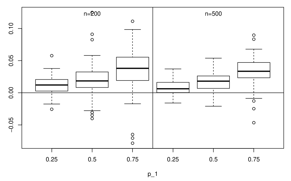
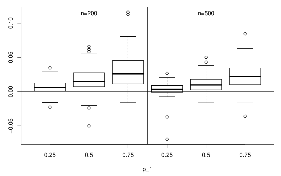
In each case, we generate a training set of size n∈{200,500}n\in\{200,500\}, and then introduce missingness by removing first component of XX independently with probability p1p_{1}.

The kernel density estimators are computed using the ks package available from CRAN. In particular, we use the kde function with a Gaussian kernel, and the diagonal bandwidth matrices were chosen using the Hpi.diag function. In the regression settings, we make use of the regpro package available from CRAN.

To measure the performance, recall that for two density functions ff and gg, say, the Total Variation distance between ff and gg is TV⁡(f,g):=12​∫ℝd|f⁡(x)−g⁡(x)|​𝑑x\mathrm{TV}(f,g):=\frac{1}{2}\int_{\mathbb{R}^{d}}|f(x)-g(x)|\,dx. We present boxplots of

TV⁡(f^0,fX)−TV⁡(f^γℳ,fX)TV⁡(f^0,fX).\frac{\mathrm{TV}(\hat{f}_{0},f_{X})-\mathrm{TV}(\hat{f}^{\mathcal{M}}_{\gamma},f_{X})}{\mathrm{TV}(\hat{f}_{0},f_{X})}. (10)

In the regression problems, we use the mean integrated squared error: for an estimate η^\hat{\eta} of η\eta that is MISE⁡(η^):=∫ℝd{η^​(x)−η⁡(x)}2​d​PX​(x)\mathrm{MISE}(\hat{\eta}):=\int_{\mathbb{R}^{d}}\{\hat{\eta}(x)-\eta(x)\}^{2}\,dP_{X}(x). Then we present boxplots of

MISE⁡(η^0,η)−MISE⁡(η^γℳ,η)MISE⁡(η^0,η).\frac{\mathrm{MISE}(\hat{\eta}_{0},\eta)-\mathrm{MISE}(\hat{\eta}^{\mathcal{M}}_{\gamma},\eta)}{\mathrm{MISE}(\hat{\eta}_{0},\eta)}. (11)
Refer to caption
Refer to caption
Refer to caption
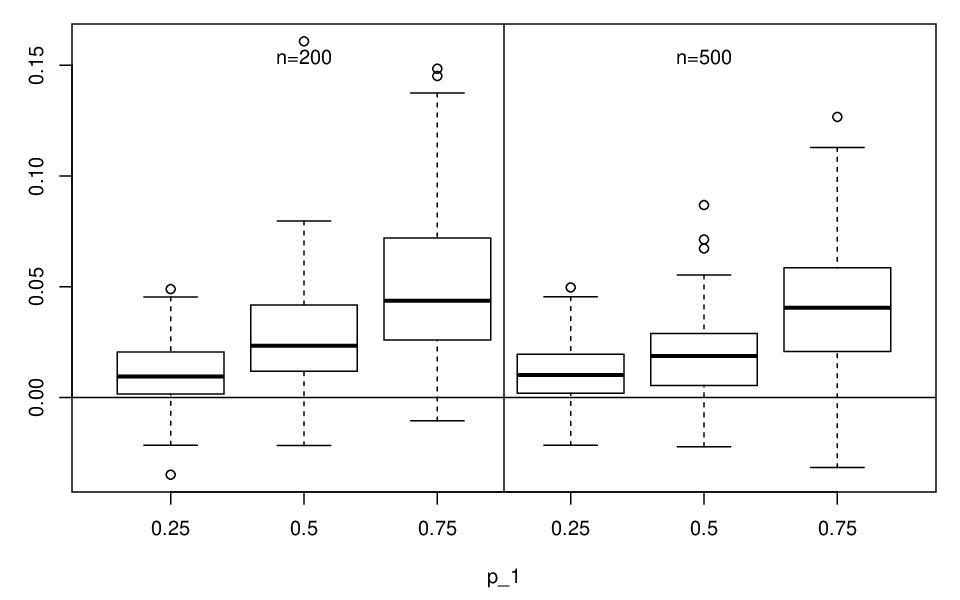
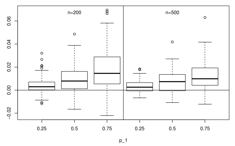
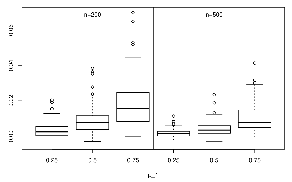
Figure 3: Boxplot of the relative performance of the CC and CAM kernel density estimators given by (10) for 100 repetitions of the experiment for density model 1 (top left), density model 2 (top right) and density model 3 (bottom).
Refer to caption
Refer to caption
Refer to caption
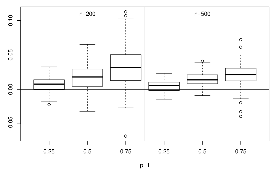
Figure 4: Boxplots of the relative performance of the CC and CAM local constant regression estimators given by (11) for 100 repetitions of the experiment for regression problem 1 (top left), regression problem 2 (top right) and regression problem 3 (bottom).

We see in Figure 3 that the CAM estimator outperforms the CC estimator in terms of total variation distance. As expected the CAM estimator leads to a greater reduction in error as the missingness probability p1p_{1} increases. On the other hand, as nn increases, the relative reduction in error is smaller. Finally, note that there are a small number of repeats of the experiment in each case where the difference in mean squared error is negative – this is likely due to the fact that we need to estimate the γ\gamma using the observed data, there is also a small Monte Carlo error.

Figure 4 shows that the CAM local constant regression estimator outperforms the CC estimator. Similarly to the density estimation problems, the CAM estimator leads to a greater reduction in error as the missingness probability p1p_{1} increases. Here we see further that for larger sample sizes, the improvement relative to using the full data set appears to decrease slightly – this is in agreement with our Theorem 5, since we only expect a second order improvement in asymptotic mean squared error.

Finally, as discussed the introduction, a popular approach to overcome issues with missing data is to impute the missing values and treat the result as a full dataset. We now compare the CAM approach to density estimation and regression with a number of state of the art imputation methods. These include mean imputation, where the missing entries for each feature are imputed with the sample mean (of the observed values) for that feature (Little and Rubin 2002, Section 4.2.1); Predictive mean matching (PMM) imputation, here the missing values are replaced by a value sampled from the observed data, where the sample is taken from the observations that are close to the observation with the missing value (Little and Rubin 2002, Section 4.3.2); and Random Forest (RF) imputation, this uses the Random Forests algorithm to predict the missing entries based on the observed data (Breiman 2002; Pantanowitz and Marwala 2009). For the latter two methods, we use multiple imputation; the missing values are imputed five times and we then take the average of the results after fitting the model on the five imputed datasets. A detailed outline of these methods can be found in Little and Rubin 2002. Our implementation utilises the mice R package available from CRAN (van Buuren et al. 2018).

In our experiments, the kernel density estimators are computed using the ks package available from CRAN. In particular, we use the kde function with a Gaussian kernel, and the diagonal bandwidth matrices were chosen using the Hpi.diag function. In the regression settings, we make use of the regpro package available from CRAN. For the imputation approaches, the corresponding kernel methods are applied to the imputed datasets.

Table 2: Average estimated total variation errors (∗103*10^{3}) for the density estimation problems and mean integrated squared error (∗103*10^{3}) for the regression problems. In each case, n=500n=500 and the first component of XX is missing with probability 1/2.
Model Full CAM CC Mean PMM RF
Density
1 4.970.02 6.070.03 6.230.03 23.770.24 6.760.10 6.860.10
2 35.310.07 40.280.08 40.580.08 101.801.04 50.211.07 38.310.31
3 51.840.10 52.490.10 52.720.10 69.660.72 52.910.34 52.850.35
Regression
1 2.740.01 4.290.02 4.350.02 6.490.10 2.650.04 6.400.11
2 2.860.02 4.120.03 4.200.03 5.820.11 12.280.23 6.020.12
3 19.290.11 29.510.19 29.840.20 61.901.01 112.221.63 24.440.46

In Table 2 we present the estimated total variation or mean integrated squared errors (with standard errors in subscript) over 100 repetitions of each experiment. For comparison, we also present the results of applying the kernel methods to the full dataset of size nn. We see that the CAM technique improves on the complete-case approach in every setting. On the other hand, as discussed in the introduction, the imputation approaches are not always successful: indeed, there are many settings here where the imputation methods lead to worse performance than the complete-case method. Notice that occasionally the imputation methods, eg. random forests in Density Model 2 and predictive mean matching in Regression Model 1, perform very well (even outperforming the full data estimator in a few cases) – it is unclear why this is the case due to the black-box nature of these approaches.

4.4 The Brandsma school dataset

In this subsection, we show how the CAM local constant regression estimator can be used in practice with the brandsma dataset available in the MICE package. The full data set consists of 4106 observations of 14 features. We simplify the problem by retaining only 4 features, namely the “verbal IQ score”, the “SES score”, “language score pre”, and “language score post”. Suppose that we are interested in predicting the verbal IQ score, YY, from the remaining features, i.e. XX is the 3-dimensional vector consisting of “SES score”, “language score pre”, and “language score post”. We remove 17 observations for which the response is missing. In the resulting dataset, we have 3464 complete-cases, 302 with m=m1=(0,1,0)Tm=m_{1}=(0,1,0)^{T}, 182 with m=m2=(0,0,1)Tm=m_{2}=(0,0,1)^{T}, and 108 with m=m3=(1,0,0)Tm=m_{3}=(1,0,0)^{T}. There are a few observations for other values of mm, but the corresponding sample sizes are all less than 20 and are therefore ignored.

In order to evaluate the performance of the CAM estimator, we take a subsample of size 1000 from the complete-cases to use as a test set (this is fixed throughout). We carry out 100 experiments. In each one, we form a training set by taking another sample of size 200 from the remaining 2464 complete-cases (this sample is different in each experiment). The 200 chosen complete-cases are then combined with the observations in Am1A_{m_{1}}, Am2A_{m_{2}} and Am3A_{m_{3}} (which are the same in every experiment). Thus, in each experiment, we have n0=200n_{0}=200, nm1=302n_{m_{1}}=302, nm2=182n_{m_{2}}=182, and nm3=108n_{m_{3}}=108.

Refer to caption
Figure 5: The average predictive MSE on the test set for the complete-case and CAM estimators for the Brandsma data application. The straight line is “y=xy=x”.

In Figure 5 we plot the average (over the test set) of {η^​(X)−Y}2\{\hat{\eta}(X)-Y\}^{2} for the complete-case and CAM estimators in each of the 100 experiments. We use a Gaussian kernel and the bandwidth was chosen using leave-one-out cross-validation. We see that the CAM estimator has a lower predictive MSE than the complete-case in 94%\% of the cases. In the remaining 6% of cases, the performance of the two estimators is similar and the discrepancy can be explained by the small sample size used to estimate the MSE. The overall average MSE (with standard errors) of the complete-case and CAM estimators were 2.28 (0.007) and 2.25 (0.006), respectively, the average improvement in MSE is 0.03 (0.002), whereas the maximum improvement over the 100 experiments was 0.09.

5 Discussion

We have seen that our proposed CAM estimator can be used to improve the complete-case estimator in a wide range of statistical problems. We conclude our paper with a discussion of few extensions of our method.

First, a key aspect of our CAM proposal is to construct θ^0,ℳ\hat{\theta}_{0,\mathcal{M}} and θ^ℳ\hat{\theta}_{\mathcal{M}}, so that θ^0,ℳ−θ^ℳ\hat{\theta}_{0,\mathcal{M}}-\hat{\theta}_{\mathcal{M}} is centered. One way to guarantee this is to use a resampling method. Let n0,m:=min⁡{n0,nm}n_{0,m}:=\min\{n_{0},n_{m}\}. Consider the sets of all subsamples (without replacement) of n0,mn_{0,m} observations from the data in A0A_{0} and AmA_{m}, respectively, denoted by A01,…,A0B0A_{0}^{1},\ldots,A_{0}^{B_{0}} and Am1,…,AmBmA_{m}^{1},\ldots,A_{m}^{B_{m}}, where B0=(n0n0,m)B_{0}={n_{0}\choose n_{0,m}} and Bm=(nmn0,m)B_{m}={n_{m}\choose n_{0,m}}. Notice that at least one of B0B_{0} and BmB_{m} will be equal to one. Then, for m∈ℳm\in\mathcal{M}, consider the two (independent) statistics θ¯0,m:=1B0​∑b=1B0θ^A0b,m\bar{\theta}_{0,m}:=\frac{1}{B_{0}}\sum_{b=1}^{B_{0}}\hat{\theta}_{A_{0}^{b},m} and θ¯m:=1Bm​∑b=1Bmθ^Amb,m\bar{\theta}_{m}:=\frac{1}{B_{m}}\sum_{b=1}^{B_{m}}\hat{\theta}_{A_{m}^{b},m}. At least in the missing completely at random setting, we have 𝔼⁡(θ¯0,m)=𝔼⁡(θ¯m)\mathbb{E}(\bar{\theta}_{0,m})=\mathbb{E}(\bar{\theta}_{m}) – each of the terms in the sums are estimators calculated on datasets of the same size. Let θ¯0,ℳ=(θ¯0,m:m∈ℳ)T\bar{\theta}_{0,\mathcal{M}}=(\bar{\theta}_{0,m}:m\in\mathcal{M})^{T}, and θ¯ℳ=(θ¯m:m∈ℳ)T\bar{\theta}_{\mathcal{M}}=(\bar{\theta}_{m}:m\in\mathcal{M})^{T}. Then, for γ∈ℝ|ℳ|\gamma\in\mathbb{R}^{|\mathcal{M}|}, define

θ¯γℳ:=θ^0−γT​(θ¯0,ℳ−θ¯ℳ).\bar{\theta}^{\mathcal{M}}_{\gamma}:=\hat{\theta}_{0}-\gamma^{T}\bigl(\bar{\theta}_{0,\mathcal{M}}-\bar{\theta}_{\mathcal{M}}\bigr).

We have the following corollary to Proposition 1, which holds for any estimation method and requires no assumptions on the distribution PP. The only restriction is that the data is MCAR.

Corollary 6.

Suppose the data is missing completely at random. Then

MSE⁡(θ¯γℳ)−MSE⁡(θ^0)=γT​Var​(θ¯0,ℳ−θ¯ℳ)​γ−2​γT​Cov​(θ^0,θ¯0,ℳ).\mathrm{MSE}(\bar{\theta}^{\mathcal{M}}_{\gamma})-\mathrm{MSE}(\hat{\theta}_{0})=\gamma^{T}\mathrm{Var}(\bar{\theta}_{0,\mathcal{M}}-\bar{\theta}_{\mathcal{M}})\gamma-2\gamma^{T}\mathrm{Cov}(\hat{\theta}_{0},\bar{\theta}_{0,\mathcal{M}}). (12)

Another consideration is the choice of the set ℳ\mathcal{M}. This choice is primarily driven by the data – in the first instance we might let ℳ=ℳ∗:={m∈{0,1}d∖{0d}:|Am|>0}\mathcal{M}=\mathcal{M}^{*}:=\{m\in\{0,1\}^{d}\setminus\{0_{d}\}:|A_{m}|>0\}. In some cases, however, we may consider using a different set ℳ\mathcal{M}. For instance, for some mm, the corresponding sample size nmn_{m} may be non-zero but small. In our numerical analysis in Section 4.3, we drop mm if |Am||A_{m}| is less than 20. Another potential option here is to use a data integration method. More specifically, let A¯m:={i∈A0c:mi≤m}\bar{A}_{m}:=\{i\in A_{0}^{c}:m_{i}\leq m\}, where the partial order on {0,1}d\{0,1\}^{d} is defined by mi≤mm_{i}\leq m if {j:mij=1}⊆{j:mj=1}\{j:m_{i}^{j}=1\}\subseteq\{j:m^{j}=1\}. Then A¯m\bar{A}_{m} is the largest set in A0cA_{0}^{c} which has complete observations for variables in {j∈{1,…​d}:mj=0}\{j\in\{1,\ldots d\}:m^{j}=0\}. Notice also that by construction A¯m\bar{A}_{m} and A0A_{0} are disjoint. To include the data integration in our CAM method, we can simply replace AmA_{m} with A¯m\bar{A}_{m}, for m∈ℳm\in\mathcal{M}. There are other options too. Suppose we have m1≠m2∈{0,1}d∖{0d}m_{1}\neq m_{2}\in\{0,1\}^{d}\setminus\{0_{d}\}, with |Am1|>0|A_{m_{1}}|>0, |Am2|=0|A_{m_{2}}|=0 and m1≤m2m_{1}\leq m_{2}. Then rather than using Am1A_{m_{1}}, we may opt to use A¯m2⊇Am1\bar{A}_{m_{2}}\supseteq A_{m_{1}} instead.

Finally we discuss the challenging non-MCAR settings. When the data is MAR or MNAR there is an additional challenge. In this case, the naive complete-case estimator will potentially be asymptotically biased. Conditionally on M1,…,MnM_{1},\ldots,M_{n}, the data in 𝒯A0,0\mathcal{T}_{A_{0},0} can be interpreted as independent and identically distributed pairs from Q0Q_{0}, that is the joint distribution of a generic pair (X,Y)|{M=0}(X,Y)|\{M=0\}. Thus, we expect the complete-case estimator θ^0\hat{\theta}_{0} to be close to θ⁡(Q0)\theta(Q_{0}) as opposed to θ⁡(P0)\theta(P_{0}). Two natural questions arise: (i) under what conditions do we have θ⁡(P0)=θ⁡(Q0)\theta(P_{0})=\theta(Q_{0}) and 𝔼⁡(θ^0,m−θ^m)≈0\mathbb{E}(\hat{\theta}_{0,m}-\hat{\theta}_{m})\approx 0 (cf. Proposition 1)?; and (ii) if the conditions in (i) do not hold, how can we adapt the CAM estimator.

A partial answer to (i) is provided by the following in the regression setting: Suppose we observe nn independent and identically distributed copies of ZM=(XM,Y)Z^{M}=(X^{M},Y) and are interested in estimating η⁡(x)=𝔼⁡(Y|X=x)\eta(x)=\mathbb{E}(Y|X=x). Assume that MM is independent of YY given XMX^{M}. (Note that this is slightly different to the missing at random condition, which assumes that MM is independent of ZZ given ZMZ^{M}.) In this case, we have that θ⁡(Q0)=𝔼⁡(Y|X=x,M=0)=𝔼⁡(Y|X=x)=θ⁡(P0)\theta(Q_{0})=\mathbb{E}(Y|X=x,M=0)=\mathbb{E}(Y|X=x)=\theta(P_{0}) and

θm​(Qm)=𝔼⁡(Y|Xm=xm,M=m)=𝔼⁡(Y|Xm=xm)=𝔼⁡(Y|Xm=xm,M=0)=θm​(Q0).\theta_{m}(Q_{m})=\mathbb{E}(Y|X^{m}=x^{m},M=m)=\mathbb{E}(Y|X^{m}=x^{m})=\mathbb{E}(Y|X^{m}=x^{m},M=0)=\theta_{m}(Q_{0}).

Thus, we can still expect that the complete-case approach will target η⁡(x)\eta(x), and moreover, can hope that Bm=𝔼⁡(θ^0,m−θ^0)≈θm​(Q0)−θm​(Qm)=0B_{m}=\mathbb{E}(\hat{\theta}_{0,m}-\hat{\theta}_{0})\approx\theta_{m}(Q_{0})-\theta_{m}(Q_{m})=0.

Relating to the problem in (ii), in the missing at random case, there are many methods that aim to correct the bias of the naive complete-case estimator; see, for instance, Little and Rubin 2002. One approach is to weight the observations according to the probability that they are (non)missing. For concreteness, we focus on one such idea, which advocates reweighting the observations according to their (inverse) propensity score – see Little and Rubin 2002. Recall that pm​(z)=pm​(x,y)=ℙ⁡(M=m|X=x,Y=y)p_{m}(z)=p_{m}(x,y)=\mathbb{P}(M=m|X=x,Y=y). Of course, pm​(x,y)p_{m}(x,y) is typically unknown, and needs to be estimated; in fact, we can only hope to estimate pm​(x,y)p_{m}(x,y) from the observed data in the missing at random setting.

Consider the UU-Statistics setting, where we are interested in estimating θ=θ⁡(P)=𝔼⁡{ϕ⁡(Z1,…,Zr)}\theta=\theta(P)=\mathbb{E}\{\phi(Z_{1},\ldots,Z_{r})\}. The complete-case approach we will in fact construct an unbiased estimator for θ⁡(Q)=𝔼⁡{ϕ⁡(Z1,…,Zr)|M1=…=Mr=0}≠θ⁡(P)\theta(Q)=\mathbb{E}\bigl\{\phi(Z_{1},\ldots,Z_{r})\big|M_{1}=\ldots=M_{r}=0\bigr\}\neq\theta(P). One solution here is to consider the Horvitz-Thompson estimators (Horvitz and Thompson 1956) in place of θ^0\hat{\theta}_{0}, θ^0,m\hat{\theta}_{0,m} and θ^m\hat{\theta}_{m}. In this problem, the complete-case analogue is

θ~0=θ~A0,0=1∑{i1,…,ir}⊆A01∏j=1rp0​(Zij)​∑{i1,…,ir}⊆A0ϕ⁡(Zi1,…,Zir)∏j=1rp0​(Zij).\tilde{\theta}_{0}=\tilde{\theta}_{A_{0},0}=\frac{1}{\sum_{\{i_{1},\ldots,i_{r}\}\subseteq A_{0}}\frac{1}{\prod_{j=1}^{r}p_{0}(Z_{i_{j}})}}\sum_{\{i_{1},\ldots,i_{r}\}\subseteq A_{0}}\frac{\phi(Z_{i_{1}},\ldots,Z_{i_{r}})}{\prod_{j=1}^{r}p_{0}(Z_{i_{j}})}.

Moreover, similar expressions can be derived for θ~0,m\tilde{\theta}_{0,m} and θ~m\tilde{\theta}_{m}. The CAM estimator can then be constructed as in the MCAR case. Of course, in practice, p0​(z)p_{0}(z) and pm​(zm)p_{m}(z^{m}) need to be estimated using the observed data. This is non-trivial, and further study in this direction is left for future work.

Acknowledgements

The work of the second author was partially supported by an NIH award 1R01GM131407.

References

  • Anderson (1957) Anderson, T. W. (1957) Maximum likelihood estimates for a multivariate normal distribution when some observations are missing. J. Amer. Statist. Assoc., 52, 200-203.
  • Biau and Devroye (2015) Biau, G. and Devroye, L. (2015) Lectures on the Nearest Neighbour Method. Springer Series in the Data Sciences, Springer International Publishing Switzerland.
  • Breiman (2002) Breiman, L. (2002) Random forests. Machine Learning, 45, 5–32.
  • Cai and Zhang (2018) Cai, T. T. and Zhang, L. (2018) High-dimensional linear discriminant analysis: optimality, adaptive algorithms and missing data. J. Roy. Statist. Soc., Ser. B, to appear.
  • Carroll et al. (1998) Carroll, R. J., Ruppert, D. and Walsh, A. H. (1998) Local estimating equations. J. Amer. Statist. Assoc., 93, 214-227.
  • Chen and Chen (2000) Chen, Y.-H. and Chen, H. (2000) A unified approach to regression analysis under double-sampling designs. J. Roy. Statist. Soc., Ser. B, 62, 449–460.
  • Dempster et al. (1977) Dempster, A. P., Laird, N. M. and Rudin, D. B. (1977) Maximum likelihood from incomplete data via the EM algorithm. J. Roy. Statist. Soc., Ser. B (with discussion), 39, 1–38.
  • Elsener and van de Geer (2018) Elsener, A. and van de Geer, S. (2018) Sparse spectral estimation with missing and corrupted measurements. Stat, 8, 1–11.
  • Fan and Gijbels (1996) Fan, J. and Gijbels, I. (1996) Local polynomial modelling and its applications, Chapman & Hall/CRC, Boca Raton, Florida.
  • Ford (1983) Ford, B. L. (1983) An overview of hot-deck procedures. In Madow, W. G., Olkin, I. and Rubin, D. B. (Eds.) Incomplete Data in Sample Surveys, Vol. 2: Theory and Bibliographies, 185–207. Academic Press, New York.
  • Fuller (1998) Fuller, W. A. (1998) Replication variance for two-phase samples. Statistica Sinica, 8, 1153–1164.
  • Horvitz and Thompson (1956) Horvitz, D. G. and Thompson, D. J. (1956) A generalization of sampling without replacement from a finite universe. J. Amer. Statist. Assoc., 47, 663–685.
  • Jiang et al. (2011) Jiang, X., Jiang, J. and Liu, Y. (2011) Nonparametric regression under double-sampling designs. J. Syst. Sci. Complex, 24, 167–175.
  • Josse and Reiter (2018) Josse, J. and Reiter, J. P. (2018) Introduction to the special section on missing data. Statistical Science, 33, 139–141.
  • Lin and Chen (2014) Lin, H.-W. and Chen Y.-H. (2014) Adjustment for missing confounders in studies based on observational databases: 2-Stage calibration combining propensity scores from primary and validation data. American Journal of Epidemiology, 180, 308–317.
  • Little and Rubin (2002) Little, R. J. A. and Rubin, D. B. (2002) Statistical analysis with missing data. Wiley, New Jersey.
  • Loh and Wainwright (2012) Loh, P.-L. and Wainwright, M. J. (2012) High-dimensional regression with noisy and missing data: provable guarantees with nonconvexity. Ann. Statist., 40, 1637–1664.
  • Molenberghs et al. (2015) Molenberghs, G., Fitzmaurice, G., Kenwood, M. G., Tsiatis, A. and Verbeke, G. (2015) Handbook of Missing Data Methodology. CRC Press, Florida.
  • Parzen (1962) Parzen, E. (1962) On estimation of a probability density function and mode. Ann. Math. Statist., 33, 1065–1076.
  • Pantanowitz and Marwala (2009) Pantanowitz, A. and Marwala, T. (2009) Missing data imputation through the use of the random forest algorithm. Adv. in Comp. Intel., 116, 53–62.
  • Rosenblatt (1956) Rosenblatt, M. (1956) Remarks on some nonparametric estimates of a density function. Ann. Math. Statist., 27, 832–837.
  • Rubin (1976) Rubin, D. B. (1976) Inference and missing data. Biometrika, 63, 581–592.
  • Tsybakov (2004) Tsybakov, A. B. (2004) Introduction to nonparametric estimation. Springer series in statistics, Springer, New York.
  • van der Vaart (1998) van der Vaart, A. (1998) Asymptotic Statistics. Cambridge University Press, Cambridge, U.K.
  • van Buuren et al. (2018) van Buuren, S., Groothuis-Oudshoorn, K., Robitzsch, A., Vink, G., Doove, L., Jolani, S., Schouten, R., Gaffert, P., Meinfelder, F. and Gray, B. (2018) mice: Multivariate imputation via chained equations. R package, available from CRAN.
  • Wahba (1990) Wahba, G. (1990) Spline Models for Observational Data. SIAM, Philadelphia, PA.
  • Wand and Jones (1995) Wand, M. P. and Jones, M. C. (1995) Kernel Smoothing. Chapman and Hall/CRC, Boca Raton, FL.
  • Yang and Ding (2019) Yang, S. and Ding, P. (2019) Combining multiple observational data sources to estimate causal effects. J. Amer. Statist. Assoc., to appear.
  • Zhang et al. (2019) Zhang, A., Brown, L. D. and Cai, T. T. (2019) Semi-supervised inference: general theory and estimation of means. Ann. Statist., 47, 2538–2566.
  • Zhu et al. (2019) Zhu, Z., Wang, T. and Samworth, R. J. (2019) High-dimensional principal component analysis with heterogeneous missingness. Preprint, ArXiv:1906.12125.

Appendix A Appendix: Technical arguments

A.1 Proofs for Section 1.1

Proof of claims in Section 1.1.

Claim 1: The statistic T=(T1,T2)T=(ν^X,1−ν^Y,1​Γ12/Γ22,ν^Y,1+ν^Y,2)TT=(T_{1},T_{2})^{T}=(\hat{\nu}_{X,1}-\hat{\nu}_{Y,1}\Gamma_{12}/\Gamma_{22},\hat{\nu}_{Y,1}+\hat{\nu}_{Y,2})^{T} is sufficient for ν=(νX,νY)T\nu=(\nu_{X},\nu_{Y})^{T}. To see this we use the factorisation criteria: let Zi=(Xi,Yi)TZ_{i}=(X_{i},Y_{i})^{T}, the full likelihood is

L⁡(ν)\displaystyle L(\nu) =∏i=1n12​π​|Γ|​exp⁡(−12​(Zi−ν)T​Γ−1​(Zi−ν))​∏i=n+12​n12​π​Γ22​exp⁡(−12​Γ22​(Yi−νY)2)\displaystyle=\prod_{i=1}^{n}\frac{1}{\sqrt{2\pi|\Gamma|}}\exp\Bigl(-\frac{1}{2}(Z_{i}-\nu)^{T}\Gamma^{-1}(Z_{i}-\nu)\Bigr)\prod_{i=n+1}^{2n}\frac{1}{\sqrt{2\pi\Gamma_{22}}}\exp\Bigl(-\frac{1}{2\Gamma_{22}}(Y_{i}-\nu_{Y})^{2}\Bigr)
=1(2​π)n​|Γ|n/2​Γ22n/2exp(−12∑i=1n(Zi−ν)TΓ−1(Zi−ν)−12​Γ22∑i=n+12​n(Yi−νY)2)\displaystyle=\frac{1}{(2\pi)^{n}|\Gamma|^{n/2}\Gamma_{22}^{n/2}}\exp\Bigl(-\frac{1}{2}\sum_{i=1}^{n}(Z_{i}-\nu)^{T}\Gamma^{-1}(Z_{i}-\nu)-\frac{1}{2\Gamma_{22}}\sum_{i=n+1}^{2n}(Y_{i}-\nu_{Y})^{2}\Bigr)
∝exp⁡(∑i=1nνT​Γ−1​Zi−12​νT​Γ−1​ν+1Γ22​∑i=n+12​nYi​νY−n​vY22​Γ22)\displaystyle\propto\exp\Bigl(\sum_{i=1}^{n}\nu^{T}\Gamma^{-1}Z_{i}-\frac{1}{2}\nu^{T}\Gamma^{-1}\nu+\frac{1}{\Gamma_{22}}\sum_{i=n+1}^{2n}Y_{i}\nu_{Y}-\frac{nv_{Y}^{2}}{2\Gamma_{22}}\Bigr)
=exp⁡(n​νT​Γ−1​(ν^X,1,ν^Y,1)T−12​νT​Γ−1​ν+1Γ22​n​ν^Y,2​νY−n​vY22​Γ22).\displaystyle=\exp\Bigl(n\nu^{T}\Gamma^{-1}(\hat{\nu}_{X,1},\hat{\nu}_{Y,1})^{T}-\frac{1}{2}\nu^{T}\Gamma^{-1}\nu+\frac{1}{\Gamma_{22}}n\hat{\nu}_{Y,2}\nu_{Y}-\frac{nv_{Y}^{2}}{2\Gamma_{22}}\Bigr).

Now write

νT​Γ−1​(ν^X,1,ν^Y,1)T=1|Γ|​{(Γ22​ν^X,1−Γ12​ν^Y,1)​νX+(Γ11​ν^Y,1−Γ12​ν^X,1)​νY}.\nu^{T}\Gamma^{-1}(\hat{\nu}_{X,1},\hat{\nu}_{Y,1})^{T}=\frac{1}{|\Gamma|}\Bigl\{(\Gamma_{22}\hat{\nu}_{X,1}-\Gamma_{12}\hat{\nu}_{Y,1})\nu_{X}+(\Gamma_{11}\hat{\nu}_{Y,1}-\Gamma_{12}\hat{\nu}_{X,1})\nu_{Y}\Bigr\}.

By collecting the coefficients of νX\nu_{X} and νY\nu_{Y}, it follows that

(ν^X,1−ν^Y,1​Γ12/Γ22,ν^X,1−ν^Y,1​Γ11/Γ12−ν^Y,2​Γ11/Γ12+ν^Y,2​Γ12/Γ22)T=(T1,T1+(Γ12Γ22−Γ11Γ12)​T2)T\Bigl(\hat{\nu}_{X,1}-\hat{\nu}_{Y,1}\Gamma_{12}/\Gamma_{22},\hat{\nu}_{X,1}-\hat{\nu}_{Y,1}\Gamma_{11}/\Gamma_{12}-\hat{\nu}_{Y,2}\Gamma_{11}/\Gamma_{12}+\hat{\nu}_{Y,2}\Gamma_{12}/{\Gamma_{22}}\Bigr)^{T}=\Bigl(T_{1},T_{1}+\bigl(\frac{\Gamma_{12}}{\Gamma_{22}}-\frac{\Gamma_{11}}{\Gamma_{12}}\bigr)T_{2}\Bigr)^{T}

is a sufficient statistic for ν\nu. Thus Claim 1 is true.

Claim 2: We have that ν~X=𝔼⁡(ν^X,1|T)\tilde{\nu}_{X}=\mathbb{E}(\hat{\nu}_{X,1}|T). To prove this, first observe that

(ν^X,1,ν^Y,1,ν^Y,2)T∼N3​((νX,νY,νY)T,Γ′),(\hat{\nu}_{X,1},\hat{\nu}_{Y,1},\hat{\nu}_{Y,2})^{T}\sim N_{3}((\nu_{X},\nu_{Y},\nu_{Y})^{T},\Gamma^{\prime}),

where

Γ′=(Γ00Γ22).\Gamma^{\prime}=\left(\begin{array}[]{c c}\Gamma&0\\ 0&\Gamma_{22}\end{array}\right).

Therefore

(ν^X,1,T1,T2)T∼N3​((νX,νX−νY​Γ12/Γ22,2​νY)T,Γ′′),(\hat{\nu}_{X,1},T_{1},T_{2})^{T}\sim N_{3}((\nu_{X},\nu_{X}-\nu_{Y}\Gamma_{12}/\Gamma_{22},2\nu_{Y})^{T},\Gamma^{\prime\prime}),

where

Γ′′=(Γ11Γ11−Γ122/Γ22Γ12Γ11−Γ122/Γ22Γ11−Γ122/Γ220Γ1202​Γ22).\Gamma^{\prime\prime}=\left(\begin{array}[]{c c c}\Gamma_{11}&\Gamma_{11}-\Gamma_{12}^{2}/\Gamma_{22}&\Gamma_{12}\\ \Gamma_{11}-\Gamma_{12}^{2}/\Gamma_{22}&\Gamma_{11}-\Gamma_{12}^{2}/\Gamma_{22}&0\\ \Gamma_{12}&0&2\Gamma_{22}\end{array}\right).

By standard Gaussian distribution theory, it follows that

𝔼⁡{ν^X,1|(T1,T2)}\displaystyle\mathbb{E}\{\hat{\nu}_{X,1}|(T_{1},T_{2})\}
=νX+(Γ11−Γ122/Γ22,Γ12)​(Γ11−Γ122/Γ22002​Γ22)−1​(T1−νX+νY​Γ12/Γ22T2−2​νY)\displaystyle=\nu_{X}+(\Gamma_{11}-\Gamma_{12}^{2}/\Gamma_{22},\Gamma_{12})\left(\begin{array}[]{c c}\Gamma_{11}-\Gamma_{12}^{2}/\Gamma_{22}&0\\ 0&2\Gamma_{22}\end{array}\right)^{-1}\left(\begin{array}[]{c}T_{1}-\nu_{X}+\nu_{Y}\Gamma_{12}/\Gamma_{22}\\ T_{2}-2\nu_{Y}\end{array}\right)
=T1−T2​Γ12/(2​Γ22)=ν~X,\displaystyle=T_{1}-T_{2}\Gamma_{12}/(2\Gamma_{22})=\tilde{\nu}_{X},

which completes the proof. ∎

A.2 Proofs of the results in Section 2

Proof of Proposition 1.

First, we have that

𝔼⁡{(θ^γℳ−θ)2−(θ^0−θ)2}\displaystyle\mathbb{E}\{(\hat{\theta}_{\gamma}^{\mathcal{M}}-\theta)^{2}-(\hat{\theta}_{0}-\theta)^{2}\}
=𝔼{(θ^γℳ−θ^0)2+2{θ^γℳ−θ^0)(θ^0−θ)}\displaystyle\hskip 60.0pt=\mathbb{E}\{(\hat{\theta}_{\gamma}^{\mathcal{M}}-\hat{\theta}_{0})^{2}+2\{\hat{\theta}_{\gamma}^{\mathcal{M}}-\hat{\theta}_{0})(\hat{\theta}_{0}-\theta)\}
=γT​𝔼​{(θ^0,ℳ−θ^ℳ)​(θ^0,ℳ−θ^ℳ)T}​γ−2​γT​𝔼​{(θ^0,ℳ−θ^ℳ)​(θ^0−θ)}.\displaystyle\hskip 60.0pt=\gamma^{T}\mathbb{E}\{(\hat{\theta}_{0,\mathcal{M}}-\hat{\theta}_{\mathcal{M}})(\hat{\theta}_{0,\mathcal{M}}-\hat{\theta}_{\mathcal{M}})^{T}\}\gamma-2\gamma^{T}\mathbb{E}\{(\hat{\theta}_{0,\mathcal{M}}-\hat{\theta}_{\mathcal{M}})(\hat{\theta}_{0}-\theta)\}.

Then, using the fact that θ^0,ℳ\hat{\theta}_{0,\mathcal{M}} and θ^ℳ\hat{\theta}_{\mathcal{M}} are independent, write

𝔼⁡{(θ^0,ℳ−θ^ℳ)​(θ^0,ℳ−θ^ℳ)T}\displaystyle\mathbb{E}\{(\hat{\theta}_{0,\mathcal{M}}-\hat{\theta}_{\mathcal{M}})(\hat{\theta}_{0,\mathcal{M}}-\hat{\theta}_{\mathcal{M}})^{T}\}
=𝔼⁡(θ^0,ℳ​θ^0,ℳT)−𝔼⁡(θ^0,ℳ​θ^ℳT)−𝔼⁡(θ^ℳ​θ^0,ℳT)+𝔼⁡(θ^ℳ​θ^ℳT)\displaystyle\hskip 60.0pt=\mathbb{E}(\hat{\theta}_{0,\mathcal{M}}\hat{\theta}_{0,\mathcal{M}}^{T})-\mathbb{E}(\hat{\theta}_{0,\mathcal{M}}\hat{\theta}_{\mathcal{M}}^{T})-\mathbb{E}(\hat{\theta}_{\mathcal{M}}\hat{\theta}_{0,\mathcal{M}}^{T})+\mathbb{E}(\hat{\theta}_{\mathcal{M}}\hat{\theta}_{\mathcal{M}}^{T})
=Var⁡(θ^0,ℳ)+Var⁡(θ^ℳ)+{𝔼⁡(θ^0,ℳ)−𝔼⁡(θ^ℳ)}​{𝔼⁡(θ^0,ℳ)−𝔼⁡(θ^ℳ)}T\displaystyle\hskip 60.0pt=\mathrm{Var}(\hat{\theta}_{0,\mathcal{M}})+\mathrm{Var}(\hat{\theta}_{\mathcal{M}})+\{\mathbb{E}(\hat{\theta}_{0,\mathcal{M}})-\mathbb{E}(\hat{\theta}_{\mathcal{M}})\}\{\mathbb{E}(\hat{\theta}_{0,\mathcal{M}})-\mathbb{E}(\hat{\theta}_{\mathcal{M}})\}^{T}
=Var⁡(θ^0,ℳ−θ^ℳ)+{𝔼⁡(θ^0,ℳ)−𝔼⁡(θ^ℳ)}​{𝔼⁡(θ^0,ℳ)−𝔼⁡(θ^ℳ)}T.\displaystyle\hskip 60.0pt=\mathrm{Var}(\hat{\theta}_{0,\mathcal{M}}-\hat{\theta}_{\mathcal{M}})+\{\mathbb{E}(\hat{\theta}_{0,\mathcal{M}})-\mathbb{E}(\hat{\theta}_{\mathcal{M}})\}\{\mathbb{E}(\hat{\theta}_{0,\mathcal{M}})-\mathbb{E}(\hat{\theta}_{\mathcal{M}})\}^{T}.

Moreover, since θ^0\hat{\theta}_{0} and θ^ℳ\hat{\theta}_{\mathcal{M}} are independent, we have

𝔼⁡{(θ^0,ℳ−θ^ℳ)​(θ^0−θ)}\displaystyle\mathbb{E}\{(\hat{\theta}_{0,\mathcal{M}}-\hat{\theta}_{\mathcal{M}})(\hat{\theta}_{0}-\theta)\} =𝔼⁡[(θ^0,ℳ−θ^ℳ)​{θ^0−𝔼⁡(θ^0)+𝔼⁡(θ^0)−θ}]\displaystyle=\mathbb{E}[(\hat{\theta}_{0,\mathcal{M}}-\hat{\theta}_{\mathcal{M}})\{\hat{\theta}_{0}-\mathbb{E}(\hat{\theta}_{0})+\mathbb{E}(\hat{\theta}_{0})-\theta\}]
=𝔼⁡[(θ^0,ℳ−θ^ℳ)​{θ^0−𝔼⁡(θ^0)}]+𝔼⁡(θ^0,ℳ−θ^ℳ)​𝔼​(θ^0−θ)\displaystyle=\mathbb{E}[(\hat{\theta}_{0,\mathcal{M}}-\hat{\theta}_{\mathcal{M}})\{\hat{\theta}_{0}-\mathbb{E}(\hat{\theta}_{0})\}]+\mathbb{E}(\hat{\theta}_{0,\mathcal{M}}-\hat{\theta}_{\mathcal{M}})\mathbb{E}(\hat{\theta}_{0}-\theta)
=Cov⁡(θ^0,ℳ,θ^0)+𝔼⁡(θ^0,ℳ−θ^ℳ)​𝔼​(θ^0−θ).\displaystyle=\mathrm{Cov}(\hat{\theta}_{0,\mathcal{M}},\hat{\theta}_{0})+\mathbb{E}(\hat{\theta}_{0,\mathcal{M}}-\hat{\theta}_{\mathcal{M}})\mathbb{E}(\hat{\theta}_{0}-\theta).

The result follows. ∎

A.3 Proofs of the results in Section 3

Proof of Theorem 2.

Note that θ^γℳ\hat{\theta}_{\gamma}^{\mathcal{M}} can be written as

θ^γℳ=(θ^0−γT​θ^0,ℳ)+γT​θ^ℳ.\displaystyle\hat{\theta}_{\gamma}^{\mathcal{M}}=(\hat{\theta}_{0}-\gamma^{T}\hat{\theta}_{0,\mathcal{M}})+\gamma^{T}\hat{\theta}_{\mathcal{M}}.

The two terms on the right hand side are independent because the former uses data in A0A_{0} and the latter uses data in A0cA_{0}^{c}. In addition, the first term on the right hand side is a UU-Statistic with kernel

ϕ~​(z1,⋯,zr)=ϕ⁡(z1,⋯,zr)−∑m∈ℳγm​ϕm​(z1m,⋯,zrm),\tilde{\phi}(z_{1},\cdots,z_{r})=\phi(z_{1},\cdots,z_{r})-\sum_{m\in\mathcal{M}}\gamma_{m}\phi_{m}(z_{1}^{m},\cdots,z_{r}^{m}),

and the second term is a linear combination of ℳ\mathcal{M} independent UU-Statistics each with kernel ϕm​(z1m,⋯,zrm)\phi_{m}(z_{1}^{m},\cdots,z_{r}^{m}). If 𝔼⁡{ϕ2​(Z1,⋯,Zr)}<∞\mathbb{E}\{\phi^{2}(Z_{1},\cdots,Z_{r})\}<\infty and 𝔼⁡{ϕm2​(Z1m,⋯,Zrm)}<∞\mathbb{E}\{\phi_{m}^{2}(Z_{1}^{m},\cdots,Z_{r}^{m})\}<\infty for a all m∈ℳm\in\mathcal{M}, we have

𝔼​{ϕ⁡(Z1,⋯,Zr)−∑m∈ℳγm​ϕm​(Z1m,⋯,Zrm)}2<∞.\mathbb{E}\Bigl\{\phi(Z_{1},\cdots,Z_{r})-\sum_{m\in\mathcal{M}}\gamma_{m}\phi_{m}(Z_{1}^{m},\cdots,Z_{r}^{m})\Bigr\}^{2}<\infty.

Let θm=𝔼⁡{ϕm​(Z1m,…,Zrm)}\theta_{m}=\mathbb{E}\{\phi_{m}\bigl(Z_{1}^{m},\ldots,Z_{r}^{m}\bigr)\} and θℳ=(θm,m∈ℳ)T\theta_{\mathcal{M}}=(\theta_{m},m\in\mathcal{M})^{T}. By classical UU-Statistics theory (see for, example, van der Vaart 1998), we have that

n0{θ^0−γTθ^0,ℳ−(θ−γTθℳ)}→dN(0,r2v0);nm(θ^m−θm)→dN(0,r2vm)\displaystyle\sqrt{n_{0}}\Bigl\{\hat{\theta}_{0}-\gamma^{T}\hat{\theta}_{0,\mathcal{M}}-(\theta-\gamma^{T}\theta_{\mathcal{M}})\Bigr\}\rightarrow^{d}N(0,r^{2}v_{0});\quad\sqrt{n_{m}}(\hat{\theta}_{m}-\theta_{m})\rightarrow^{d}N(0,r^{2}v_{m})

as n→∞n\rightarrow\infty, where v0:=Cov⁡{ϕ~​(Z1,Z2,⋯,Zr),ϕ~​(Z1,Zr+2,⋯,Z2​r)}v_{0}:=\mathrm{Cov}\{\tilde{\phi}(Z_{1},Z_{2},\cdots,Z_{r}),\tilde{\phi}(Z_{1},Z_{r+2},\cdots,Z_{2r})\} and
vm:=Cov⁡{ϕm​(Z1m,Z2m,⋯,Zrm),ϕ⁡(Z1m,Zr+2m,⋯,Z2​rm)}v_{m}:=\mathrm{Cov}\{\phi_{m}(Z_{1}^{m},Z_{2}^{m},\cdots,Z_{r}^{m}),\phi(Z_{1}^{m},Z_{r+2}^{m},\cdots,Z_{2r}^{m})\}.

Now, by the independence of θ^0−γT​θ^0,ℳ\hat{\theta}_{0}-\gamma^{T}\hat{\theta}_{0,\mathcal{M}} and θ^ℳ\hat{\theta}_{\mathcal{M}}, and noting that limn→∞nmn0=qmq0\lim_{n\rightarrow\infty}\frac{n_{m}}{n_{0}}=\frac{q_{m}}{q_{0}}, we have

n0(θ^γℳ−θ)→dN(0,r2(v0+∑m∈ℳγmqm−1q0vm)).\sqrt{n_{0}}\bigl(\hat{\theta}_{\gamma}^{\mathcal{M}}-\theta\bigr)\rightarrow^{d}N\Bigl(0,r^{2}\bigl(v_{0}+\sum_{m\in\mathcal{M}}\gamma_{m}q_{m}^{-1}q_{0}v_{m}\bigr)\Bigr).

Finally, by the definition of ϕ~​(z1,⋯,zr)\tilde{\phi}(z_{1},\cdots,z_{r}) we can derive that v0+∑m∈ℳγm​qm−1​q0​vm=ψ1+γT​Λ1​γ−2​γT​Ω1v_{0}+\sum_{m\in\mathcal{M}}\gamma_{m}q_{m}^{-1}q_{0}v_{m}=\psi_{1}+\gamma^{T}\Lambda_{1}\gamma-2\gamma^{T}\Omega_{1}. This completes the proof of the theorem. ∎

Proof of Theorem 3.

First, we formally define our UU-Statistic estimates of ΩU\Omega_{U} and ΛU\Lambda_{U}. We have

Ω^U,m\displaystyle\hat{\Omega}_{U,m} :=12​(n04​r−2)∑{i1,…,i4​r−2}⊆A0[{ϕ(Zi1,…,Zir)−ϕ(Zi2​r,…,Zi3​r−1)}\displaystyle:=\frac{1}{2{n_{0}\choose 4r-2}}\sum_{\{i_{1},\ldots,i_{4r-2}\}\subseteq A_{0}}\Bigl[\bigl\{\phi\bigl(Z_{i_{1}},\ldots,Z_{i_{r}}\bigr)-\phi\bigl(Z_{i_{2r}},\ldots,Z_{i_{3r-1}}\bigr)\bigr\}
{ϕm(Zi1m,Zir+1m,…,Zi2​r−1m)−ϕm(Zi2​rm,Zi3​rm,…,Zi4​r−2m)}].\displaystyle\hskip 120.0pt\bigl\{\phi_{m}\bigl(Z^{m}_{i_{1}},Z^{m}_{i_{r+1}},\ldots,Z^{m}_{i_{2r-1}}\bigr)-\phi_{m}\bigl(Z_{i_{2r}}^{m},Z_{i_{3r}}^{m},\ldots,Z_{i_{4r-2}}^{m}\bigr)\bigr\}\Bigr]. (13)

Moreover

Λ^U,m,m\displaystyle\hat{\Lambda}_{U,m,m} :=(1+n0nm)12​(n0+nm4​r−2)∑{i1,…,i4​r−2}⊆A0∪Am[{ϕm(Zi1m,…,Zirm)−ϕm(Zi2​rm,…,Zi3​r−1m)}\displaystyle:=\Bigl(1+\frac{n_{0}}{n_{m}}\Bigr)\frac{1}{2{n_{0}+n_{m}\choose 4r-2}}\sum_{\{i_{1},\ldots,i_{4r-2}\}\subseteq A_{0}\cup A_{m}}\Bigl[\bigl\{\phi_{m}\bigl(Z_{i_{1}}^{m},\ldots,Z_{i_{r}}^{m}\bigr)-\phi_{m}\bigl(Z_{i_{2r}}^{m},\ldots,Z_{i_{3r-1}}^{m}\bigr)\bigr\}
{ϕm(Zi1m,Zir+1m,…,Zi2​r−1m)−ϕm(Zi2​rm,Zi3​rm,…,Zi4​r−2m)}];\displaystyle\hskip 90.0pt\bigl\{\phi_{m}\bigl(Z_{i_{1}}^{m},Z_{i_{r+1}}^{m},\ldots,Z_{i_{2r-1}}^{m}\bigr)-\phi_{m}\bigl(Z_{i_{2r}}^{m},Z_{i_{3r}}^{m},\ldots,Z_{i_{4r-2}}^{m}\bigr)\bigr\}\Bigr]; (14)

and

Λ^U,m1,m2\displaystyle\hat{\Lambda}_{U,m_{1},m_{2}} :=12​(n0+nm1,24​r−2)∑{i1,…,i4​r−2}⊆A0∪Am1,2[{ϕm1(Zi1m1,…,Zirm1)−ϕm1(Zi2​rm1,…,Zi3​r−1m1)}\displaystyle:=\frac{1}{2{n_{0}+n_{m_{1,2}}\choose 4r-2}}\sum_{\{i_{1},\ldots,i_{4r-2}\}\subseteq A_{0}\cup A_{m_{1,2}}}\Bigl[\bigl\{\phi_{m_{1}}\bigl(Z_{i_{1}}^{m_{1}},\ldots,Z_{i_{r}}^{m_{1}}\bigr)-\phi_{m_{1}}\bigl(Z_{i_{2r}}^{m_{1}},\ldots,Z_{i_{3r-1}}^{m_{1}}\bigr)\bigr\}
{ϕm2(Zi1m2,Zir+1m2,…,Zi2​r−1m2)−ϕm2(Zi2​rm2,Zi3​rm2,…,Zi4​r−2m2)}].\displaystyle\hskip 60.0pt\bigl\{\phi_{m_{2}}\bigl(Z_{i_{1}}^{m_{2}},Z_{i_{r+1}}^{m_{2}},\ldots,Z_{i_{2r-1}}^{m_{2}}\bigr)-\phi_{m_{2}}\bigl(Z_{i_{2r}}^{m_{2}},Z_{i_{3r}}^{m_{2}},\ldots,Z_{i_{4r-2}}^{m_{2}}\bigr)\bigr\}\Bigr]. (15)

Then, by classical UU-Statistics theory (van der Vaart 1998, Theorem 12.3), we can prove that Λ^\hat{\Lambda} and Ω^\hat{\Omega} are consistent estimators of Λ\Lambda and Ω\Omega, respectively. Then the consistency of γ^\hat{\gamma} to γ∗\gamma^{*} follows automatically. Next note that

n0​(θ^γ^ℳ−θ)−n0​(θ^γℳ−θ)=n0​(θ^γ^ℳ−θ^γℳ)=n0​(θ^0,ℳ−θ^ℳ)T​(γ^−γ∗).\displaystyle\sqrt{n_{0}}(\hat{\theta}_{\hat{\gamma}}^{\mathcal{M}}-\theta)-\sqrt{n_{0}}(\hat{\theta}_{\gamma}^{\mathcal{M}}-\theta)=\sqrt{n_{0}}(\hat{\theta}_{\hat{\gamma}}^{\mathcal{M}}-\hat{\theta}_{\gamma}^{\mathcal{M}})=\sqrt{n_{0}}(\hat{\theta}_{0,\mathcal{M}}-\hat{\theta}_{\mathcal{M}})^{T}(\hat{\gamma}-\gamma^{*}).

By the proof of Theorem 2, the vector n0​(θ^0,ℳ−θ^ℳ)\sqrt{n_{0}}(\hat{\theta}_{0,\mathcal{M}}-\hat{\theta}_{\mathcal{M}}) is jointly asymptotically normal. Since γ^−γ∗=op​(1)\hat{\gamma}-\gamma^{*}=o_{p}(1), it follows from the Slutsky’s theorem that

n0(θ^γ^ℳ−θ)−n0(θ^γℳ−θ)→p0.\sqrt{n_{0}}(\hat{\theta}_{\hat{\gamma}}^{\mathcal{M}}-\theta)-\sqrt{n_{0}}(\hat{\theta}_{\gamma}^{\mathcal{M}}-\theta)\rightarrow^{p}0.

This, together with Theorem 2, completes the proof of the theorem. ∎

A.4 Conditions and proofs for the results in Section 4

We first formally state our assumptions. In the following, L>0L>0 is some universal constant.

A​​ 1.

Suppose that PXP_{X} and, for m∈{0,1}d∖{(1,…,1)T}m\in\{0,1\}^{d}\setminus\{(1,\ldots,1)^{T}\}, the marginal XmX^{m} distribution PXmP_{X^{m}} have densities fXf_{X}, and fXmf_{X^{m}}, respectively, that satisfy |fX​(z1)−fX​(z2)|≤L​‖z1−z2‖|f_{X}(z_{1})-f_{X}(z_{2})|\leq L\|z_{1}-z_{2}\|, for all z1,z2∈ℝdz_{1},z_{2}\in\mathbb{R}^{d}, and, for each m∈{0,1}d∖{(1,…,1)T}m\in\{0,1\}^{d}\setminus\{(1,\ldots,1)^{T}\}, we have |fXm​(z1m)−fXm​(z2m)|≤L​‖z1m−z2m‖|f_{X^{m}}(z_{1}^{m})-f_{X^{m}}(z_{2}^{m})|\leq L\|z_{1}^{m}-z_{2}^{m}\|, for all z1m,z2m∈ℝdmz_{1}^{m},z_{2}^{m}\in\mathbb{R}^{d_{m}}.

A​​ 2.

Suppose the kernel is such that K¯:=supz∈ℝd(1+‖z‖)​K​(z)<∞\bar{K}:=\sup_{z\in\mathbb{R}^{d}}(1+\|z\|)K(z)<\infty, and that μ0=μ0​(K):=∫ℝdK⁡(z)​𝑑z=1\mu_{0}=\mu_{0}(K):=\int_{\mathbb{R}^{d}}K(z)\,dz=1, μ1=μ1​(K):=∫ℝd‖z‖​K​(z)​𝑑z<∞\mu_{1}=\mu_{1}(K):=\int_{\mathbb{R}^{d}}\|z\|K(z)\,dz<\infty. We also ask that ν=ν⁡(K):=∫ℝdK2​(z)​𝑑z<∞\nu=\nu(K):=\int_{\mathbb{R}^{d}}K^{2}(z)\,dz<\infty. Moreover, for each m∈ℳm\in\mathcal{M}, we have K¯m:=supz∈ℝdm(1+‖z‖)​Km​(z)<∞\bar{K}_{m}:=\sup_{z\in\mathbb{R}^{d_{m}}}(1+\|z\|)K_{m}(z)<\infty, μ0,m=μ0,m​(Km):=∫ℝdmKm​(z)​𝑑z<∞\mu_{0,m}=\mu_{0,m}(K_{m}):=\int_{\mathbb{R}^{d_{m}}}K_{m}(z)\,dz<\infty, μ1,m=μ1,m​(Km):=∫ℝdm‖z‖​Km​(z)​𝑑z<∞\mu_{1,m}=\mu_{1,m}(K_{m}):=\int_{\mathbb{R}^{d_{m}}}\|z\|K_{m}(z)\,dz<\infty, and νm=νm​(Km):=∫ℝdmKm2​(z)​𝑑z<∞\nu_{m}=\nu_{m}(K_{m}):=\int_{\mathbb{R}^{d_{m}}}K_{m}^{2}(z)\,dz<\infty. Finally for m1≠m2∈ℳm_{1}\neq m_{2}\in\mathcal{M}, letting m1,2=pmax⁡{m1,m2}∈{0,1}dm^{1,2}=\mathrm{pmax}\{m_{1},m_{2}\}\in\{0,1\}^{d} and m1,2=pmim⁡{m1,m2}∈{0,1}dm_{1,2}=\mathrm{pmim}\{m_{1},m_{2}\}\in\{0,1\}^{d} denote the entrywise maximums and minimums, respectively, of m1m_{1} and m2m_{2}, finally we suppose that νm1,m2=νm1,m2​(Km1,Km2):=∫ℝdm1,2Km1​(zm1)​Km2​(zm2)​d​zm1,2<∞.\nu_{m_{1},m_{2}}=\nu_{m_{1},m_{2}}(K_{m_{1}},K_{m_{2}}):=\int_{\mathbb{R}^{d_{m_{1,2}}}}K_{m_{1}}(z^{m_{1}})K_{m_{2}}(z^{m_{2}})\,dz^{m_{1,2}}<\infty.

A​​ 3.

We have that |η⁡(z1)−η⁡(z2)|≤L​‖z1−z2‖|\eta(z_{1})-\eta(z_{2})|\leq L\|z_{1}-z_{2}\|, for all z1,z2∈ℝdz_{1},z_{2}\in\mathbb{R}^{d}, and, for each m∈ℳm\in\mathcal{M}, |ηm​(z1m)−ηm​(z2m)|≤L​‖z1m−z2m‖|\eta_{m}(z_{1}^{m})-\eta_{m}(z_{2}^{m})|\leq L\|z_{1}^{m}-z_{2}^{m}\|, for all z1m,z2m∈ℝdmz_{1}^{m},z_{2}^{m}\in\mathbb{R}^{d_{m}}.

A​​ 4.

For each m∈ℳm\in\mathcal{M}, we have |τm​(z1m)−τm​(z2m)|≤L​‖z1m−z2m‖|\tau_{m}(z_{1}^{m})-\tau_{m}(z_{2}^{m})|\leq L\|z_{1}^{m}-z_{2}^{m}\|, for all z1m,z2m∈ℝdmz_{1}^{m},z_{2}^{m}\in\mathbb{R}^{d_{m}}. Finally, we ask, for all m1,m2∈ℳm_{1},m_{2}\in\mathcal{M}, that |τm1,m2​(z1m1,2)−τm1,m2​(z2m1,2)|≤L​‖z1m1,2−z2m1,2‖|\tau_{m_{1},m_{2}}(z_{1}^{m_{1,2}})-\tau_{m_{1},m_{2}}(z_{2}^{m_{1,2}})|\leq L\|z_{1}^{m_{1,2}}-z_{2}^{m_{1,2}}\|, for all z1m1,2,z2m1,2∈ℝdm1,2z_{1}^{m_{1,2}},z_{2}^{m_{1,2}}\in\mathbb{R}^{d_{m_{1,2}}}.

Proof of Theorem 4.

First, we have

𝔼⁡[{f^γℳ−fX​(x)}2−{f^0−fX​(x)}2]\displaystyle\mathbb{E}[\{\hat{f}_{\gamma}^{\mathcal{M}}-f_{X}(x)\}^{2}-\{\hat{f}_{0}-f_{X}(x)\}^{2}]
=𝔼⁡[(f^γℳ​(x)−f^0)2+2​(f^γℳ−f^0)​{f^0−fX​(x)}]\displaystyle\hskip 60.0pt=\mathbb{E}[(\hat{f}_{\gamma}^{\mathcal{M}}(x)-\hat{f}_{0})^{2}+2(\hat{f}_{\gamma}^{\mathcal{M}}-\hat{f}_{0})\{\hat{f}_{0}-f_{X}(x)\}]
=γT​𝔼​{(f^0,ℳ−f^ℳ)​(f^0,ℳ−f^ℳ)T}​γ−2​γT​𝔼​[(f^0,ℳ−f^ℳ)​{f^0−fX​(x)}].\displaystyle\hskip 60.0pt=\gamma^{T}\mathbb{E}\{(\hat{f}_{0,\mathcal{M}}-\hat{f}_{\mathcal{M}})(\hat{f}_{0,\mathcal{M}}-\hat{f}_{\mathcal{M}})^{T}\}\gamma-2\gamma^{T}\mathbb{E}[(\hat{f}_{0,\mathcal{M}}-\hat{f}_{\mathcal{M}})\{\hat{f}_{0}-f_{X}(x)\}].

Now observe that, for each m∈ℳm\in\mathcal{M},

𝔼⁡(f^0,m−f^m)=1n0​hdm​∑i∈A0𝔼⁡{Km​(Xim−xmh)}−1nm​hdm​∑i∈Am𝔼⁡{Km​(Xim−xmh)}=0.\mathbb{E}(\hat{f}_{0,m}-\hat{f}_{m})=\frac{1}{n_{0}h^{d_{m}}}\sum_{i\in A_{0}}\mathbb{E}\Bigl\{K_{m}\Bigl(\frac{X_{i}^{m}-x^{m}}{h}\Bigr)\Bigr\}-\frac{1}{n_{m}h^{d_{m}}}\sum_{i\in A_{m}}\mathbb{E}\Bigl\{K_{m}\Bigl(\frac{X_{i}^{m}-x^{m}}{h}\Bigr)\Bigr\}=0.

Thus, using also that f^0,ℳ\hat{f}_{0,\mathcal{M}} and f^ℳ\hat{f}_{\mathcal{M}} are independent, we can write

𝔼⁡{(f^0,ℳ−f^ℳ)​(f^0,ℳ−f^ℳ)T}\displaystyle\mathbb{E}\{(\hat{f}_{0,\mathcal{M}}-\hat{f}_{\mathcal{M}})(\hat{f}_{0,\mathcal{M}}-\hat{f}_{\mathcal{M}})^{T}\}
=𝔼⁡[{f^0,ℳ−𝔼⁡(f^0,ℳ)+f^ℳ−𝔼⁡(f^ℳ)}​{f^0,ℳ−𝔼⁡(f^0,ℳ)+f^ℳ−𝔼⁡(f^ℳ)}T]\displaystyle\hskip 30.0pt=\mathbb{E}[\{\hat{f}_{0,\mathcal{M}}-\mathbb{E}(\hat{f}_{0,\mathcal{M}})+\hat{f}_{\mathcal{M}}-\mathbb{E}(\hat{f}_{\mathcal{M}})\}\{\hat{f}_{0,\mathcal{M}}-\mathbb{E}(\hat{f}_{0,\mathcal{M}})+\hat{f}_{\mathcal{M}}-\mathbb{E}(\hat{f}_{\mathcal{M}})\}^{T}]
=Cov⁡(f^0,ℳ)+Cov⁡(f^ℳ).\displaystyle\hskip 30.0pt=\mathrm{Cov}(\hat{f}_{0,\mathcal{M}})+\mathrm{Cov}(\hat{f}_{\mathcal{M}}). (16)

It remains to show that Cov⁡(f^0,ℳ)+Cov⁡(f^ℳ)=ΛD​(1+o⁡(1))\mathrm{Cov}(\hat{f}_{0,\mathcal{M}})+\mathrm{Cov}(\hat{f}_{\mathcal{M}})=\Lambda_{D}(1+o(1)) and 𝔼⁡[(f^0,ℳ−f^ℳ)​{f^0−fX​(x)}]=ΩD​(1+o⁡(1))\mathbb{E}[(\hat{f}_{0,\mathcal{M}}-\hat{f}_{\mathcal{M}})\{\hat{f}_{0}-f_{X}(x)\}]=\Omega_{D}(1+o(1)).

For the diagonal terms in the covariances in (A.4), we have

Var⁡(f^0,m)+Var⁡(f^m)\displaystyle\mathrm{Var}(\hat{f}_{0,m})+\mathrm{Var}(\hat{f}_{m}) =1h2​dm​(1n0+1nm)​Var​{Km​(Xm−xmh)}\displaystyle=\frac{1}{h^{2d_{m}}}\Bigl(\frac{1}{n_{0}}+\frac{1}{n_{m}}\Bigr)\mathrm{Var}\Bigl\{K_{m}\Bigl(\frac{X^{m}-x^{m}}{h}\Bigr)\Bigr\}
=1h2​dm(1n0+1nm)[∫ℝdmKm2(zm−xmh)fXm(zm)dzm\displaystyle=\frac{1}{h^{2d_{m}}}\Bigl(\frac{1}{n_{0}}+\frac{1}{n_{m}}\Bigr)\biggl[\int_{\mathbb{R}^{d_{m}}}K_{m}^{2}\Bigl(\frac{z^{m}-x^{m}}{h}\Bigr)f_{X^{m}}(z^{m})\,dz^{m}
−{∫ℝdmKm(zm−xmh)fXm(zm)dzm}2].\displaystyle\hskip 120.0pt-\Bigl\{\int_{\mathbb{R}^{d_{m}}}K_{m}\Bigl(\frac{z^{m}-x^{m}}{h}\Bigr)f_{X^{m}}(z^{m})\,dz^{m}\Bigr\}^{2}\biggr].

After making the substitution um=zm−xmhu^{m}=\frac{z^{m}-x^{m}}{h} and using assumptions A1 and A2, we deduce that

|∫ℝdmKm2​(zm−xmh)​fXm​(zm)​d​zm−hdm​fXm​(xm)​νm|\displaystyle\Bigl|\int_{\mathbb{R}^{d_{m}}}K_{m}^{2}\Bigl(\frac{z^{m}-x^{m}}{h}\Bigr)f_{X^{m}}(z^{m})\,dz^{m}-h^{d_{m}}f_{X^{m}}(x^{m})\nu_{m}\Bigr|
≤hdm​∫ℝdmKm2​(um)​|fXm​(xm+h​um)−fXm​(xm)|​d​um≤L​hdm+1​K¯m​μ1,m.\displaystyle\hskip 60.0pt\leq h^{d_{m}}\int_{\mathbb{R}^{d_{m}}}K_{m}^{2}(u^{m})|f_{X^{m}}(x^{m}+hu^{m})-f_{X^{m}}(x^{m})|\,du^{m}\leq Lh^{d_{m}+1}\bar{K}_{m}\mu_{1,m}.

Whereas

|∫ℝdmKm​(zm−xmh)​fXm​(zm)​d​zm−hdm​fXm​(xm)​μ0,m|\displaystyle\Bigl|\int_{\mathbb{R}^{d_{m}}}K_{m}\Bigl(\frac{z^{m}-x^{m}}{h}\Bigr)f_{X^{m}}(z^{m})\,dz^{m}-h^{d_{m}}f_{X^{m}}(x^{m})\mu_{0,m}\Bigr|
≤hdm​∫ℝdmKm​(um)​|fXm​(xm+h​um)−fXm​(xm)|​d​um≤L​hdm+1​μ1,m.\displaystyle\hskip 60.0pt\leq h^{d_{m}}\int_{\mathbb{R}^{d_{m}}}K_{m}(u^{m})|f_{X^{m}}(x^{m}+hu^{m})-f_{X^{m}}(x^{m})|\,du^{m}\leq Lh^{d_{m}+1}\mu_{1,m}. (17)

It follows that

Var⁡(f^0,m)+Var⁡(f^m)=fXm​(xm)​νmhdm​(1n0+1nm)​{1+o⁡(1)},\mathrm{Var}(\hat{f}_{0,m})+\mathrm{Var}(\hat{f}_{m})=\frac{f_{X^{m}}(x^{m})\nu_{m}}{h^{d_{m}}}\Bigl(\frac{1}{n_{0}}+\frac{1}{n_{m}}\Bigr)\{1+o(1)\},

as n→∞n\rightarrow\infty, uniformly for h∈[n−β,n−α]h\in[n^{-\beta},n^{-\alpha}].

For the off-diagonal terms in (A.4): first, for m1≠m2∈ℳm_{1}\neq m_{2}\in\mathcal{M}, we have that Cov⁡(f^m1,f^m2)=0,\mathrm{Cov}(\hat{f}_{m_{1}},\hat{f}_{m_{2}})=0, since Am1A_{m_{1}} and Am2A_{m_{2}} are disjoint for m1≠m2m_{1}\neq m_{2}. For the remaining terms, we have

Cov⁡(f^0,m1,f^0,m2)\displaystyle\mathrm{Cov}(\hat{f}_{0,m_{1}},\hat{f}_{0,m_{2}})
=1n0​hdm1+dm2​Cov​{Km1​(Xm1−xm1h),Km2​(Xm2−xm2h)}\displaystyle\hskip 10.0pt=\frac{1}{n_{0}h^{d_{m_{1}}+d_{m_{2}}}}\mathrm{Cov}\Bigl\{K_{m_{1}}\Bigl(\frac{X^{m_{1}}-x^{m_{1}}}{h}\Bigr),K_{m_{2}}\Bigl(\frac{X^{m_{2}}-x^{m_{2}}}{h}\Bigr)\Bigr\}
=1n0​hdm1+dm2​{∫ℝdKm1​(zm1−xm1h)​Km2​(zm2−xm2h)​fX​(z)​𝑑z}\displaystyle\hskip 10.0pt=\frac{1}{n_{0}h^{d_{m_{1}}+d_{m_{2}}}}\biggl\{\int_{\mathbb{R}^{d}}K_{m_{1}}\Bigl(\frac{z^{m_{1}}-x^{m_{1}}}{h}\Bigr)K_{m_{2}}\Bigl(\frac{z^{m_{2}}-x^{m_{2}}}{h}\Bigr)f_{X}(z)\,dz\biggr\}
−1n0​hdm1+dm2​{∫ℝdKm1​(zm1−xm1h)​fX​(z)​𝑑z}​{∫ℝdKm2​(zm2−xm2h)​fX​(z)​𝑑z}.\displaystyle\hskip 40.0pt-\frac{1}{n_{0}h^{d_{m_{1}}+d_{m_{2}}}}\biggl\{\int_{\mathbb{R}^{d}}K_{m_{1}}\Bigl(\frac{z^{m_{1}}-x^{m_{1}}}{h}\Bigr)f_{X}(z)\,dz\biggr\}\biggl\{\int_{\mathbb{R}^{d}}K_{m_{2}}\Bigl(\frac{z^{m_{2}}-x^{m_{2}}}{h}\Bigr)f_{X}(z)\,dz\biggr\}.

As above, we make the substitution u=z−xhu=\frac{z-x}{h}, which gives

∫ℝdKm1​(zm1−xm1h)​Km2​(zm2−xm2h)​fX​(z)​𝑑z\displaystyle\int_{\mathbb{R}^{d}}K_{m_{1}}\Bigl(\frac{z^{m_{1}}-x^{m_{1}}}{h}\Bigr)K_{m_{2}}\Bigl(\frac{z^{m_{2}}-x^{m_{2}}}{h}\Bigr)f_{X}(z)\,dz
=hd​∫ℝdKm1​(um1)​Km2​(um2)​fX​(x+h​u)​𝑑u\displaystyle\hskip 90.0pt=h^{d}\int_{\mathbb{R}^{d}}K_{m_{1}}(u^{m_{1}})K_{m_{2}}(u^{m_{2}})f_{X}(x+hu)\,du
=hd​∫ℝdm1,2∫ℝd−dm1,2Km1​(um1)​Km1​(um2)​fX​(x+h​u)​d​u1d−m1,2​d​um1,2\displaystyle\hskip 90.0pt=h^{d}\int_{\mathbb{R}^{d_{m_{1,2}}}}\int_{\mathbb{R}^{d-d_{m_{1,2}}}}K_{m_{1}}(u^{m_{1}})K_{m_{1}}(u^{m_{2}})f_{X}(x+hu)\,du^{1_{d}-m_{1,2}}du^{m_{1,2}}
=hd​∫ℝdm1,2Km1​(um1)​Km2​(um2)​∫ℝd−dm1,2fX​(x+h​u)​d​u1d−m1,2​d​um1,2\displaystyle\hskip 90.0pt=h^{d}\int_{\mathbb{R}^{d_{m_{1,2}}}}K_{m_{1}}(u^{m_{1}})K_{m_{2}}(u^{m_{2}})\int_{\mathbb{R}^{d-d_{m_{1,2}}}}f_{X}(x+hu)\,du^{1_{d}-m_{1,2}}du^{m_{1,2}}
=hdm1,2​∫ℝdm1,2Km1​(um1)​Km2​(um2)​fXm1,2​(xm1,2+h​um1,2)​d​um1,2\displaystyle\hskip 90.0pt=h^{d_{m_{1,2}}}\int_{\mathbb{R}^{d_{m_{1,2}}}}K_{m_{1}}(u^{m_{1}})K_{m_{2}}(u^{m_{2}})f_{X^{m_{1,2}}}(x^{m_{1,2}}+hu^{m_{1,2}})\,du^{m_{1,2}}
=hdm1,2​νm1,m2​fXm1,2​(xm1,2)​{1+o⁡(1)},\displaystyle\hskip 90.0pt=h^{d_{m_{1,2}}}\nu_{m_{1},m_{2}}f_{X^{m_{1,2}}}(x^{m_{1,2}})\{1+o(1)\},

uniformly for h∈[n−β,n−α]h\in[n^{-\beta},n^{-\alpha}]. It follows from the previous calculation and (A.4), that

Cov⁡(f^0,m1,f^0,m2)=νm1,m2​fXm1,2​(xm1,2)n0​hdm1,2​{1+o⁡(1)},\mathrm{Cov}(\hat{f}_{0,m_{1}},\hat{f}_{0,m_{2}})=\frac{\nu_{m_{1},m_{2}}f_{X^{m_{1,2}}}(x^{m_{1,2}})}{n_{0}h^{d_{m^{1,2}}}}\{1+o(1)\},

uniformly for h∈[n−β,n−α]h\in[n^{-\beta},n^{-\alpha}]. This proves that first claim that Cov⁡(f^0,ℳ)+Cov⁡(f^ℳ)=ΛD​(1+o⁡(1))\mathrm{Cov}(\hat{f}_{0,\mathcal{M}})+\mathrm{Cov}(\hat{f}_{\mathcal{M}})=\Lambda_{D}(1+o(1)).

Finally, since f^0\hat{f}_{0} and f^ℳ\hat{f}_{\mathcal{M}} are independent, we have that

𝔼⁡[(f^0,ℳ−f^ℳ)​{f^0−fX​(x)}]\displaystyle\mathbb{E}[(\hat{f}_{0,\mathcal{M}}-\hat{f}_{\mathcal{M}})\{\hat{f}_{0}-f_{X}(x)\}] =𝔼⁡[(f^0,ℳ−f^ℳ)​{f^0−𝔼⁡(f^0)+𝔼⁡(f^0)−fX​(x)}]\displaystyle=\mathbb{E}[(\hat{f}_{0,\mathcal{M}}-\hat{f}_{\mathcal{M}})\{\hat{f}_{0}-\mathbb{E}(\hat{f}_{0})+\mathbb{E}(\hat{f}_{0})-f_{X}(x)\}]
=𝔼⁡[{f^0,ℳ−𝔼⁡(f^0,ℳ)−f^ℳ+𝔼⁡(f^ℳ)}​{f^0−𝔼⁡(f^0)}]\displaystyle=\mathbb{E}[\{\hat{f}_{0,\mathcal{M}}-\mathbb{E}(\hat{f}_{0,\mathcal{M}})-\hat{f}_{\mathcal{M}}+\mathbb{E}(\hat{f}_{\mathcal{M}})\}\{\hat{f}_{0}-\mathbb{E}(\hat{f}_{0})\}]
=Cov⁡(f^0,ℳ,f^0)+Cov⁡(f^ℳ,f^0)=Cov⁡(f^0,ℳ,f^0).\displaystyle=\mathrm{Cov}(\hat{f}_{0,\mathcal{M}},\hat{f}_{0})+\mathrm{Cov}(\hat{f}_{\mathcal{M}},\hat{f}_{0})=\mathrm{Cov}(\hat{f}_{0,\mathcal{M}},\hat{f}_{0}).

Then, reusing the covariance calculation above, for m∈ℳm\in\mathcal{M}, we have

Cov⁡(f^0,f^0,m)\displaystyle\mathrm{Cov}(\hat{f}_{0},\hat{f}_{0,m}) =1n0​hd+dm​Cov​{K⁡(X−xh),Km​(Xm−xmh)}=ν0,m​fX​(x)n0​hdm​{1+o⁡(1)},\displaystyle=\frac{1}{n_{0}h^{d+d_{m}}}\mathrm{Cov}\Bigl\{K\Bigl(\frac{X-x}{h}\Bigr),K_{m}\Bigl(\frac{X^{m}-x^{m}}{h}\Bigr)\Bigr\}=\frac{\nu_{0,m}f_{X}(x)}{n_{0}h^{d_{m}}}\{1+o(1)\},

uniformly for h∈[n−β,n−α]h\in[n^{-\beta},n^{-\alpha}]. This completes the proof of the second claim and hence concludes the proof of the theorem. ∎

Proof of Theorem 5.

First, conditionally on the observed data, we have

𝔼[{η^γℳ−η(x)}2|X1m1,…,Xnmn]−𝔼[{η^0−η(x)}2|X1m1,…,Xnmn]\displaystyle\mathbb{E}[\{\hat{\eta}^{\mathcal{M}}_{\gamma}-\eta(x)\}^{2}|X_{1}^{m_{1}},\ldots,X_{n}^{m_{n}}]-\mathbb{E}[\{\hat{\eta}_{0}-\eta(x)\}^{2}|X_{1}^{m_{1}},\ldots,X_{n}^{m_{n}}]
=𝔼{(η^γℳ−η^0)2|X1m1,…,Xnmn}+2𝔼[{η^0−η(x)}{η^γℳ−η^0}|X1m1,…,Xnmn].\displaystyle\hskip 30.0pt=\mathbb{E}\{(\hat{\eta}^{\mathcal{M}}_{\gamma}-\hat{\eta}_{0})^{2}|X_{1}^{m_{1}},\ldots,X_{n}^{m_{n}}\}+2\mathbb{E}[\{\hat{\eta}_{0}-\eta(x)\}\{\hat{\eta}^{\mathcal{M}}_{\gamma}-\hat{\eta}_{0}\}|X_{1}^{m_{1}},\ldots,X_{n}^{m_{n}}]. (18)

We analyse the two terms in (A.4) separately. We first introduce some notation and facts that will be used repeatedly in the proof. Recall that we can write the local constant estimator as a linear function of the responses Y[n]:=(Y1,…,Yn)T∈ℝnY_{[n]}:=(Y_{1},\ldots,Y_{n})^{T}\in\mathbb{R}^{n}. Indeed, let

WA,m=WA,m,h,Km:=(Km(X1m−xmh)𝟙{1∈A},…,Km(Xnm−xmh)𝟙{n∈A})T.W_{A,m}=W_{A,m,h,K_{m}}:=\biggl(K_{m}\Bigl(\frac{X^{m}_{1}-x^{m}}{h}\Bigr)\mathbbm{1}_{\{1\in A\}},\ldots,K_{m}\Bigl(\frac{X^{m}_{n}-x^{m}}{h}\Bigr)\mathbbm{1}_{\{n\in A\}}\biggr)^{T}. (19)

Then η^A,m​(xm)=HA,m,h,KmT​Y[n]\hat{\eta}_{A,m}(x^{m})=H_{A,m,h,K_{m}}^{T}Y_{[n]}, where HA,m=HA,m,h,Km:=(∑i=1nWA,m,i)−1​WA,mH_{A,m}=H_{A,m,h,K_{m}}:=(\sum_{i=1}^{n}W_{A,m,i})^{-1}W_{A,m}. For simplicity of presentation, write H0=HA0,0H_{0}=H_{A_{0},0}, H0,m=HA0,mH_{0,m}=H_{A_{0},m} and Hm=HAm,mH_{m}=H_{A_{m},m}, and let H0,ℳ=(H0,m:m∈ℳ)H_{0,\mathcal{M}}=(H_{0,m}:m\in\mathcal{M}) be the n×|ℳ|n\times|\mathcal{M}| matrix with columns H0,mH_{0,m}, for m∈ℳm\in\mathcal{M}, and similarly let Hℳ=(Hm:m∈ℳ)∈ℝn×|ℳ|H_{\mathcal{M}}=(H_{m}:m\in\mathcal{M})\in\mathbb{R}^{n\times|\mathcal{M}|}.

Next, let E=𝔼⁡(Y[n]|X1m1,…,Xnmn)=(ηm1​(X1m1),…,ηmn​(Xnmn))TE=\mathbb{E}(Y_{[n]}|X_{1}^{m_{1}},\ldots,X_{n}^{m_{n}})=\bigl(\eta_{m_{1}}(X_{1}^{m_{1}}),\ldots,\eta_{m_{n}}(X_{n}^{m_{n}})\bigr)^{T} be the conditional expectation of the responses, and let Γ:=diag⁡{τm1​(X1m1),…,τmn​(Xnmn)}\Gamma:=\mathrm{diag}\{\tau_{m_{1}}(X_{1}^{m_{1}}),\ldots,\tau_{m_{n}}(X_{n}^{m_{n}})\}. Further, let Γ∗=diag⁡{τm1​(xm1),…,τmn​(xmn)}\Gamma^{*}=\mathrm{diag}\{\tau_{m_{1}}(x^{m_{1}}),\ldots,\tau_{m_{n}}(x^{m_{n}})\} and E∗={ηm1​(xm1),…,ηmn​(xmn)}TE^{*}=\{\eta_{m_{1}}(x^{m_{1}}),\ldots,\eta_{m_{n}}(x^{m_{n}})\}^{T}. We will make use of the following facts (i) 1nT​HA,m=11_{n}^{T}H_{A,m}=1; (ii) E∗T​H0=η⁡(x)E^{*T}H_{0}=\eta(x), (iii) HmT​E∗=ηm​(xm)H_{m}^{T}E^{*}=\eta_{m}(x^{m}), (iv) H0,mT​E∗=η⁡(x)H_{0,m}^{T}E^{*}=\eta(x), (v) HmT​Γ∗​Hm=τm​(xm)​HmT​HmH_{m}^{T}\Gamma^{*}H_{m}=\tau_{m}(x^{m})H_{m}^{T}H_{m}, (vi) H0,mT​Γ∗=0H_{0,m}^{T}\Gamma^{*}=0, (vii) Γ​H0=Γ∗​H0=0\Gamma H_{0}=\Gamma^{*}H_{0}=0 and (viii) HℳT​H0=0H_{\mathcal{M}}^{T}H_{0}=0.

Furthermore, we claim that, for m∈ℳm\in\mathcal{M}, the following results are true

H0T​H0,m=ν0,mμ0,m​fXm​(xm)​n0​hdm​{1+Op​(h)};H_{0}^{T}H_{0,m}=\frac{\nu_{0,m}}{\mu_{0,m}f_{X^{m}}(x^{m})n_{0}h^{d_{m}}}\{1+O_{p}(h)\}; (20)
H0,mT​H0,m=νmμ0,m2​fXm​(xm)​n0​hdm​{1+Op​(h)};H_{0,m}^{T}H_{0,m}=\frac{\nu_{m}}{\mu^{2}_{0,m}f_{X^{m}}(x^{m})n_{0}h^{d_{m}}}\{1+O_{p}(h)\}; (21)

and

HmT​Hm=νmμ0,m2​fXm​(xm)​nm​hdm​{1+Op​(h)},H_{m}^{T}H_{m}=\frac{\nu_{m}}{\mu^{2}_{0,m}f_{X^{m}}(x^{m})n_{m}h^{d_{m}}}\{1+O_{p}(h)\}, (22)

uniformly for h∈[n−β,n−α]h\in[n^{-\beta},n^{-\alpha}]. Furthermore, for m1≠m2∈ℳm_{1}\neq m_{2}\in\mathcal{M}, we have

H0,m1T​H0,m2=νm1,m2​fXm1,2​(xm1,2)μ0,m1​fXm1​(xm1)​μ0,m2​fXm2​(xm2)​n0​hdm1,2​{1+Op​(h)};H_{0,m_{1}}^{T}H_{0,m_{2}}=\frac{\nu_{m_{1},m_{2}}f_{X^{m_{1,2}}}(x^{m_{1,2}})}{\mu_{0,m_{1}}f_{X^{m_{1}}}(x^{m_{1}})\mu_{0,m_{2}}f_{X^{m_{2}}}(x^{m_{2}})n_{0}h^{d_{m^{1,2}}}}\{1+O_{p}(h)\}; (23)

uniformly for h∈[n−β,n−α]h\in[n^{-\beta},n^{-\alpha}]. To see (20), write

H0T​H0,m\displaystyle H_{0}^{T}H_{0,m} =∑i∈A0K⁡(Xi−xh)​Km​(Xim−xmh)∑i∈A0K⁡(Xi−xh)​∑i∈A0Km​(Xim−xmh)\displaystyle=\frac{\sum_{i\in A_{0}}K\bigl(\frac{X_{i}-x}{h}\bigr)K_{m}\bigl(\frac{X^{m}_{i}-x^{m}}{h}\bigr)}{\sum_{i\in A_{0}}K\bigl(\frac{X_{i}-x}{h}\bigr)\sum_{i\in A_{0}}K_{m}\bigl(\frac{X^{m}_{i}-x^{m}}{h}\bigr)}
=1n02​hd+dm​∑i∈A0K⁡(Xi−xh)​Km​(Xim−xmh)1n0​hd​∑i∈A0K⁡(Xi−xh)​1n0​hdm​∑i∈A0Km​(Xim−xmh).\displaystyle=\frac{\frac{1}{n_{0}^{2}h^{d+d_{m}}}\sum_{i\in A_{0}}K\bigl(\frac{X_{i}-x}{h}\bigr)K_{m}\bigl(\frac{X^{m}_{i}-x^{m}}{h}\bigr)}{\frac{1}{n_{0}h^{d}}\sum_{i\in A_{0}}K\bigl(\frac{X_{i}-x}{h}\bigr)\frac{1}{n_{0}h^{d_{m}}}\sum_{i\in A_{0}}K_{m}\bigl(\frac{X^{m}_{i}-x^{m}}{h}\bigr)}. (24)

We consider the numerator and denominator above separately. For the numerator, observe that

𝔼⁡{1n02​hd+dm​∑i∈A0K⁡(Xi−xh)​Km​(Xim−xmh)}\displaystyle\mathbb{E}\Bigl\{\frac{1}{n_{0}^{2}h^{d+d_{m}}}\sum_{i\in A_{0}}K\bigl(\frac{X_{i}-x}{h}\bigr)K_{m}\bigl(\frac{X^{m}_{i}-x^{m}}{h}\bigr)\Bigr\}
=1n0​hd+dm​∫ℝdK⁡(z−xh)​Km​(zm−xmh)​fX​(z)​𝑑z\displaystyle\hskip 90.0pt=\frac{1}{n_{0}h^{d+d_{m}}}\int_{\mathbb{R}^{d}}K\bigl(\frac{z-x}{h}\bigr)K_{m}\bigl(\frac{z^{m}-x^{m}}{h}\bigr)f_{X}(z)\,dz
=1n0​hdm​∫ℝdK⁡(u)​Km​(um)​fX​(x+h​u)​𝑑z\displaystyle\hskip 90.0pt=\frac{1}{n_{0}h^{d_{m}}}\int_{\mathbb{R}^{d}}K(u)K_{m}(u^{m})f_{X}(x+hu)\,dz
=ν0,m​fX​(x)n0​hdm+1n0​hdm​∫ℝdK⁡(u)​Km​(um)​{fX​(x+h​u)−fX​(x)}​𝑑z.\displaystyle\hskip 90.0pt=\frac{\nu_{0,m}f_{X}(x)}{n_{0}h^{d_{m}}}+\frac{1}{n_{0}h^{d_{m}}}\int_{\mathbb{R}^{d}}K(u)K_{m}(u^{m})\{f_{X}(x+hu)-f_{X}(x)\}\,dz.

Moreover, by Assumptions A1 and A2, we have

∫ℝd|K⁡(u)​Km​(um)​{fX​(x+h​u)−fX​(x)}|​𝑑z≤L​h​∫ℝdK⁡(u)​Km​(um)|u|𝑑u≤L​h​μ1​K¯m.\int_{\mathbb{R}^{d}}\Bigl|K(u)K_{m}(u^{m})\{f_{X}(x+hu)-f_{X}(x)\}\Bigr|\,dz\leq Lh\int_{\mathbb{R}^{d}}K(u)K_{m}(u^{m})\|u\|\,du\leq Lh\mu_{1}\bar{K}_{m}.

Hence, using Markov’s inequality, the numerator in (A.4) admits the following expression

1n02​hd+dm​∑i∈A0K⁡(Xi−xh)​Km​(Xim−xmh)=ν0,m​fX​(x)n0​hdm+Op​(1/(n0​hdm−1)),\frac{1}{n_{0}^{2}h^{d+d_{m}}}\sum_{i\in A_{0}}K\Bigl(\frac{X_{i}-x}{h}\Bigr)K_{m}\Bigl(\frac{X^{m}_{i}-x^{m}}{h}\Bigr)=\frac{\nu_{0,m}f_{X}(x)}{n_{0}h^{d_{m}}}+O_{p}(1/(n_{0}h^{d_{m}-1})),

uniformly for h∈[n−β,n−α]h\in[n^{-\beta},n^{-\alpha}]. For the denominator, by appealing to similar arguments to those in the proof of Theorem 4, we have that

1n0​hd​∑i∈A0K⁡(Xi−xh)=fX​(x)+Op​(h),\frac{1}{n_{0}h^{d}}\sum_{i\in A_{0}}K\Bigl(\frac{X_{i}-x}{h}\Bigr)=f_{X}(x)+O_{p}(h),

and

1n0​hdm​∑i∈A0Km​(Xim−xmh)=fXm​(xm)​μ0,m+Op​(h),\frac{1}{n_{0}h^{d_{m}}}\sum_{i\in A_{0}}K_{m}\Bigl(\frac{X^{m}_{i}-x^{m}}{h}\Bigr)=f_{X^{m}}(x^{m})\mu_{0,m}+O_{p}(h),

uniformly for h∈[n−β,n−α]h\in[n^{-\beta},n^{-\alpha}]. The claim in (20) then follows by Slutsky’s Theorem. Moreover, the claims in (21) and (22) follow by the same argument with only minor changes. To see (23), observe that

𝔼⁡{1n02​hdm1+dm2​∑i∈A0Km1​(Xim1−xm1h)​Km2​(Xim2−xm2h)}\displaystyle\mathbb{E}\Bigl\{\frac{1}{n_{0}^{2}h^{d_{m_{1}}+d_{m_{2}}}}\sum_{i\in A_{0}}K_{m_{1}}\bigl(\frac{X^{m_{1}}_{i}-x^{m_{1}}}{h}\bigr)K_{m_{2}}\bigl(\frac{X^{m_{2}}_{i}-x^{m_{2}}}{h}\bigr)\Bigr\}
=1n0​hdm1+dm2​∫ℝdKm1​(zm1−xm1h)​Km2​(zm2−xm2h)​fX​(z)​𝑑z\displaystyle\hskip 60.0pt=\frac{1}{n_{0}h^{d_{m_{1}}+d_{m_{2}}}}\int_{\mathbb{R}^{d}}K_{m_{1}}\bigl(\frac{z^{m_{1}}-x^{m_{1}}}{h}\bigr)K_{m_{2}}\bigl(\frac{z^{m_{2}}-x^{m_{2}}}{h}\bigr)f_{X}(z)\,dz
=1n0​hdm1+dm2​∫ℝdm1,2Km1​(zm1−xm1h)​Km2​(zm2−xm2h)​fXm1,2​(zm1,2)​d​zm1,2\displaystyle\hskip 60.0pt=\frac{1}{n_{0}h^{d_{m_{1}}+d_{m_{2}}}}\int_{\mathbb{R}^{d_{m_{1,2}}}}K_{m_{1}}\bigl(\frac{z^{m_{1}}-x^{m_{1}}}{h}\bigr)K_{m_{2}}\bigl(\frac{z^{m_{2}}-x^{m_{2}}}{h}\bigr)f_{X^{m_{1,2}}}(z^{m_{1,2}})\,dz^{m_{1,2}}
=1n0​hdm1+dm2−dm1,2​∫ℝdm1,2Km1​(um1)​Km2​(um2)​fXm1,2​(xm1,2+h​um1,2)​d​um1,2\displaystyle\hskip 60.0pt=\frac{1}{n_{0}h^{d_{m_{1}}+d_{m_{2}}-d_{m_{1,2}}}}\int_{\mathbb{R}^{d_{m_{1,2}}}}K_{m_{1}}(u^{m_{1}})K_{m_{2}}(u^{m_{2}})f_{X^{m_{1,2}}}(x^{m_{1,2}}+hu^{m_{1,2}})\,du^{m_{1,2}}
=νm1,m2​fXm1,2​(xm1,2)n0​hdm1,2+O⁡(1/(n0​hdm1,2−1)),\displaystyle\hskip 60.0pt=\frac{\nu_{m_{1},m_{2}}f_{X^{m_{1,2}}}(x^{m_{1,2}})}{n_{0}h^{d_{m^{1,2}}}}+O(1/(n_{0}h^{d_{m^{1,2}}-1})),

uniformly for h∈[n−β,n−α]h\in[n^{-\beta},n^{-\alpha}]. In the last step above we have used the fact that, by Assumptions A1 and A2, we have

∫ℝdm1,2Km1​(um1)​Km2​(um2)​{fXm1,2​(xm1,2+h​um1,2)−fXm1,2​(xm1,2)}​d​um1,2\displaystyle\int_{\mathbb{R}^{d_{m_{1,2}}}}K_{m_{1}}(u^{m_{1}})K_{m_{2}}(u^{m_{2}})\{f_{X^{m_{1,2}}}(x^{m_{1,2}}+hu^{m_{1,2}})-f_{X^{m_{1,2}}}(x^{m_{1,2}})\}\,du^{m_{1,2}}
≤L​h​∫ℝdm1,2Km1​(um1)​Km2​(um2)​‖um1,2‖​d​um1,2\displaystyle\hskip 20.0pt\leq Lh\int_{\mathbb{R}^{d_{m_{1,2}}}}K_{m_{1}}(u^{m_{1}})K_{m_{2}}(u^{m_{2}})\|u^{m_{1,2}}\|\,du^{m_{1,2}}
≤L​h​∫ℝdm1,2Km1​(um1)​Km2​(um2)​(‖um1‖+‖um2‖)​d​um1,2≤L​h​(μ1,m1​K¯m2+μ1,m2​K¯m1).\displaystyle\hskip 20.0pt\leq Lh\int_{\mathbb{R}^{d_{m_{1,2}}}}K_{m_{1}}(u^{m_{1}})K_{m_{2}}(u^{m_{2}})(\|u^{m_{1}}\|+\|u^{m_{2}}\|)\,du^{m_{1,2}}\leq Lh(\mu_{1,m_{1}}\bar{K}_{m_{2}}+\mu_{1,m_{2}}\bar{K}_{m_{1}}).

The claim in (23) then follows by similar arguments used to prove (20). We now return to the main argument.

Part I: the first term in (A.4): By definition of Y[n]Y_{[n]} we have

𝔼⁡(Y[n]​Y[n]T|X1m1,…,Xnmn)=E​ET+σ2​In×n+Γ.\mathbb{E}(Y_{[n]}Y_{[n]}^{T}|X_{1}^{m_{1}},\ldots,X_{n}^{m_{n}})=EE^{T}+\sigma^{2}I_{n\times n}+\Gamma.

It follows from the definitions of η^γℳ\hat{\eta}_{\gamma}^{\mathcal{M}} and η^0\hat{\eta}_{0} that the first term in (A.4) takes the form

𝔼{(η^γℳ−η^0)2|X1m1,…,Xnmn}\displaystyle\mathbb{E}\{(\hat{\eta}_{\gamma}^{\mathcal{M}}-\hat{\eta}_{0})^{2}|X_{1}^{m_{1}},\ldots,X_{n}^{m_{n}}\} =γT​(H0,ℳT−HℳT)​(E​ET+σ2​In×n+Γ)​(H0,ℳ−Hℳ)​γ\displaystyle=\gamma^{T}\bigl(H_{0,\mathcal{M}}^{T}-H_{\mathcal{M}}^{T}\bigr)(EE^{T}+\sigma^{2}I_{n\times n}+\Gamma)\bigl(H_{0,\mathcal{M}}-H_{\mathcal{M}}\bigr)\gamma
=γT​ΛR​γ+R1+R2,\displaystyle=\gamma^{T}\Lambda_{R}\gamma+R_{1}+R_{2}, (25)

where

R1:=γT​HℳT​(Γ−Γ∗)​Hℳ​γR_{1}:=\gamma^{T}H_{\mathcal{M}}^{T}(\Gamma-\Gamma^{*})H_{\mathcal{M}}\gamma

and

R2:={γT​(H0,ℳT−HℳT)​E}2+σ2​γT​H0,ℳT​H0,ℳ​γ+γT​HℳT​(σ2​I+Γ∗)​Hℳ​γ−γT​ΛR​γ.R_{2}:=\{\gamma^{T}(H_{0,\mathcal{M}}^{T}-H_{\mathcal{M}}^{T})E\}^{2}+\sigma^{2}\gamma^{T}H_{0,\mathcal{M}}^{T}H_{0,\mathcal{M}}\gamma+\gamma^{T}H_{\mathcal{M}}^{T}(\sigma^{2}I+\Gamma^{*})H_{\mathcal{M}}\gamma-\gamma^{T}\Lambda_{\mathrm{R}}\gamma.

Here we have used that H0,ℳT​(Γ−Γ∗)​H0,ℳ=0H_{0,\mathcal{M}}^{T}(\Gamma-\Gamma^{*})H_{0,\mathcal{M}}=0. We next show that both R1R_{1} and R2R_{2} are small order terms.

To bound R1R_{1}: By assumption A4, we have that

|τm​(xim)−τm​(xm)|≤L​‖xim−xm‖.|\tau_{m}(x_{i}^{m})-\tau_{m}(x^{m})|\leq L\|x_{i}^{m}-x^{m}\|.

Moreover, similarly to (22), by Assumption A2, we have

HmT​diag​(‖Ximi−xmi‖,i=1,…,n)​Hm\displaystyle H_{m}^{T}\mathrm{diag}(\|X_{i}^{m_{i}}-x^{m_{i}}\|,i=1,\ldots,n)H_{m} =∑i∈Am‖Xim−xm‖​Km2​(Xim−xmh)∑i∈AmKm​(Xim−xmh)​∑i∈AmKm​(Xim−xmh)\displaystyle=\frac{\sum_{i\in A_{m}}\|X_{i}^{m}-x^{m}\|K_{m}^{2}\bigl(\frac{X^{m}_{i}-x^{m}}{h}\bigr)}{\sum_{i\in A_{m}}K_{m}\bigl(\frac{X_{i}^{m}-x^{m}}{h}\bigr)\sum_{i\in A_{m}}K_{m}\bigl(\frac{X^{m}_{i}-x^{m}}{h}\bigr)}
≤1nm2​h2​dm−1​∑i∈AmK¯m​Km​(Xim−xmh){1nm​hdm​∑i∈AmKm​(Xim−xmh)}2\displaystyle\leq\frac{\frac{1}{n_{m}^{2}h^{2d_{m}-1}}\sum_{i\in A_{m}}\bar{K}_{m}K_{m}\bigl(\frac{X^{m}_{i}-x^{m}}{h}\bigr)}{\{\frac{1}{n_{m}h^{d_{m}}}\sum_{i\in A_{m}}K_{m}\bigl(\frac{X^{m}_{i}-x^{m}}{h}\bigr)\}^{2}}
=Op​(1nm​hdm−1).\displaystyle=O_{p}\bigl(\frac{1}{n_{m}h^{d_{m}-1}}\bigr).

uniformly for h∈[n−β,n−α]h\in[n^{-\beta},n^{-\alpha}]. Thus

|R1|\displaystyle|R_{1}| =|γT​HℳT​(Γ−Γ∗)​Hℳ​γ|\displaystyle=\Bigl|\gamma^{T}H_{\mathcal{M}}^{T}(\Gamma-\Gamma^{*})H_{\mathcal{M}}\gamma\Bigr|
≤∑m∈ℳγm2​HmT​diag​(‖Ximi−xmi‖,i=1,…,n)​Hm=Op​(∑m∈ℳγm2nm​hdm−1),\displaystyle\leq\sum_{m\in\mathcal{M}}\gamma_{m}^{2}H_{m}^{T}\mathrm{diag}(\|X_{i}^{m_{i}}-x^{m_{i}}\|,i=1,\ldots,n)H_{m}=O_{p}\Bigl(\sum_{m\in\mathcal{M}}\frac{\gamma_{m}^{2}}{n_{m}h^{d_{m}-1}}\Bigr),

uniformly for h∈[n−β,n−α]h\in[n^{-\beta},n^{-\alpha}].

To bound R2R_{2}: First we decompose R2R_{2} into the sum of three terms. To that end, let

R21\displaystyle R_{21} :={γT​(H0,ℳT−HℳT)​E}2−∑m∈ℳγm2​νm​τm​(xm)μ0,m2​fXm​(xm)​n0​hdm\displaystyle:=\{\gamma^{T}(H_{0,\mathcal{M}}^{T}-H_{\mathcal{M}}^{T})E\}^{2}-\sum_{m\in\mathcal{M}}\frac{\gamma_{m}^{2}\nu_{m}\tau_{m}(x^{m})}{\mu^{2}_{0,m}f_{X^{m}}(x^{m})n_{0}h^{d_{m}}}
−∑m1≠m2∈ℳγm1​γm2​τm1,m2​(xm1,2)​νm1,m2​fXm1,2​(xm1,2)μ0,m1​fXm1​(xm1)​μ0,m2​fXm2​(xm2)​n0​hdm1,2;\displaystyle\hskip 120.0pt-\sum_{m_{1}\neq m_{2}\in\mathcal{M}}\frac{\gamma_{m_{1}}\gamma_{m_{2}}\tau_{m_{1},m_{2}}(x^{m_{1,2}})\nu_{m_{1},m_{2}}f_{X^{m_{1,2}}}(x^{m_{1,2}})}{\mu_{0,m_{1}}f_{X^{m_{1}}}(x^{m_{1}})\mu_{0,m_{2}}f_{X^{m_{2}}}(x^{m_{2}})n_{0}h^{d_{m^{1,2}}}};
R22\displaystyle R_{22} :=σ2​γT​H0,ℳT​H0,ℳ​γ−∑m∈ℳγm2​νm​σ2μ0,m2​fXm​(xm)​n0​hdm\displaystyle:=\sigma^{2}\gamma^{T}H_{0,\mathcal{M}}^{T}H_{0,\mathcal{M}}\gamma-\sum_{m\in\mathcal{M}}\frac{\gamma_{m}^{2}\nu_{m}\sigma^{2}}{\mu^{2}_{0,m}f_{X^{m}}(x^{m})n_{0}h^{d_{m}}}
−∑m1≠m2∈ℳγm1​γm2​σ2​νm1,m2​fXm1,2​(xm1,2)μ0,m1​fXm1​(xm1)​μ0,m2​fXm2​(xm2)​n0​hdm1,2;\displaystyle\hskip 120.0pt-\sum_{m_{1}\neq m_{2}\in\mathcal{M}}\frac{\gamma_{m_{1}}\gamma_{m_{2}}\sigma^{2}\nu_{m_{1},m_{2}}f_{X^{m_{1,2}}}(x^{m_{1,2}})}{\mu_{0,m_{1}}f_{X^{m_{1}}}(x^{m_{1}})\mu_{0,m_{2}}f_{X^{m_{2}}}(x^{m_{2}})n_{0}h^{d_{m^{1,2}}}};

and

R23:=γT​HℳT​(σ2​I+Γ∗)​Hℳ​γ−∑m∈ℳγm2​νm​{σ2+τm​(xm)}μ0,m2​fXm​(xm)​nm​hdm.\displaystyle R_{23}:=\gamma^{T}H_{\mathcal{M}}^{T}(\sigma^{2}I+\Gamma^{*})H_{\mathcal{M}}\gamma-\sum_{m\in\mathcal{M}}\frac{\gamma_{m}^{2}\nu_{m}\{\sigma^{2}+\tau_{m}(x^{m})\}}{\mu^{2}_{0,m}f_{X^{m}}(x^{m})n_{m}h^{d_{m}}}.

Note that R2=R21+R22+R23R_{2}=R_{21}+R_{22}+R_{23}, since

γT​ΛR​γ\displaystyle\gamma^{T}\Lambda_{\mathrm{R}}\gamma =∑m∈ℳγm2​νm​{σ2+τm​(xm)}μ0,m2​fXm​(xm)​n0​hdm+∑m∈ℳγm2​νm​{σ2+τm​(xm)}μ0,m2​fXm​(xm)​nm​hdm.\displaystyle=\sum_{m\in\mathcal{M}}\frac{\gamma_{m}^{2}\nu_{m}\{\sigma^{2}+\tau_{m}(x^{m})\}}{\mu^{2}_{0,m}f_{X^{m}}(x^{m})n_{0}h^{d_{m}}}+\sum_{m\in\mathcal{M}}\frac{\gamma_{m}^{2}\nu_{m}\{\sigma^{2}+\tau_{m}(x^{m})\}}{\mu^{2}_{0,m}f_{X^{m}}(x^{m})n_{m}h^{d_{m}}}.
−∑m1≠m2∈ℳγm1​γm2​{σ2+τm1,m2​(xm1,2)}​νm1,m2​fXm1,2​(xm1,2)μ0,m1​fXm1​(xm1)​μ0,m2​fXm2​(xm2)​n0​hdm1,2.\displaystyle\hskip 120.0pt-\sum_{m_{1}\neq m_{2}\in\mathcal{M}}\frac{\gamma_{m_{1}}\gamma_{m_{2}}\{\sigma^{2}+\tau_{m_{1},m_{2}}(x^{m_{1,2}})\}\nu_{m_{1},m_{2}}f_{X^{m_{1,2}}}(x^{m_{1,2}})}{\mu_{0,m_{1}}f_{X^{m_{1}}}(x^{m_{1}})\mu_{0,m_{2}}f_{X^{m_{2}}}(x^{m_{2}})n_{0}h^{d_{m^{1,2}}}}.

We now bound R21R_{21}, R22R_{22} and R23R_{23} in turn.

To bound R21R_{21}: Write Em=(ηm​(X1m),…​ηm​(Xnm))TE_{m}=(\eta_{m}(X_{1}^{m}),\ldots\eta_{m}(X_{n}^{m}))^{T} and let δm=E−Em\delta_{m}=E-E_{m}. Then Hm​δm=0H_{m}\delta_{m}=0 and

γT​(H0,ℳT−HℳT)​E\displaystyle\gamma^{T}\bigl(H_{0,\mathcal{M}}^{T}-H_{\mathcal{M}}^{T}\bigr)E =∑m∈ℳγm​(H0,mT−HmT)​E\displaystyle=\sum_{m\in\mathcal{M}}\gamma_{m}\bigl(H_{0,m}^{T}-H_{m}^{T}\bigr)E
=∑m∈ℳγm​(H0,mT−HmT)​(E−Em+Em)\displaystyle=\sum_{m\in\mathcal{M}}\gamma_{m}\bigl(H_{0,m}^{T}-H_{m}^{T}\bigr)(E-E_{m}+E_{m})
=∑m∈ℳγm​{H0,mT​δm+(H0,mT−HmT)​Em}.\displaystyle=\sum_{m\in\mathcal{M}}\gamma_{m}\bigl\{H_{0,m}^{T}\delta_{m}+(H_{0,m}^{T}-H_{m}^{T})E_{m}\bigr\}. (26)

For m∈ℳm\in\mathcal{M}, using the fact H0,mT​1n=HmT​1n=1H_{0,m}^{T}1_{n}=H_{m}^{T}1_{n}=1 we have that

|(H0,mT−HmT)​Em|=|(H0,mT−HmT)​{Em−ηm​(xm)​1n}|\displaystyle|(H_{0,m}^{T}-H_{m}^{T})E_{m}|=|(H_{0,m}^{T}-H_{m}^{T})\{E_{m}-\eta_{m}(x^{m})1_{n}\}|
=|1n0​hdm​∑i∈A0Km​(Xim−xmh)​{ηm​(Xim)−ηm​(xm)}1n0​hdm​∑i∈A0Km​(Xim−xmh)\displaystyle=\Bigl|\frac{\frac{1}{n_{0}h^{d_{m}}}\sum_{i\in A_{0}}K_{m}\bigl(\frac{X^{m}_{i}-x^{m}}{h}\bigr)\{\eta_{m}(X_{i}^{m})-\eta_{m}(x^{m})\}}{\frac{1}{n_{0}h^{d_{m}}}\sum_{i\in A_{0}}K_{m}\bigl(\frac{X^{m}_{i}-x^{m}}{h}\bigr)}
−1nm​hdm​∑i∈AmKm​(Xim−xmh)​{ηm​(Xim)−ηm​(xm)}1nm​hdm​∑i∈AmKm​(Xim−xmh)|\displaystyle\hskip 120.0pt-\frac{\frac{1}{n_{m}h^{d_{m}}}\sum_{i\in A_{m}}K_{m}\bigl(\frac{X^{m}_{i}-x^{m}}{h}\bigr)\{\eta_{m}(X_{i}^{m})-\eta_{m}(x^{m})\}}{\frac{1}{n_{m}h^{d_{m}}}\sum_{i\in A_{m}}K_{m}\bigl(\frac{X^{m}_{i}-x^{m}}{h}\bigr)}\Bigr|
=1f^0,m​f^m​n0​nm​h2​dm|∑i∈A0,j∈Am[Km(Xim−xmh){ηm(Xim)−ηm(xm)}Km(Xjm−xmh)\displaystyle=\frac{1}{\hat{f}_{0,m}\hat{f}_{m}n_{0}n_{m}h^{2d_{m}}}\Bigl|\sum_{i\in A_{0},j\in A_{m}}\Bigl[K_{m}\Bigl(\frac{X^{m}_{i}-x^{m}}{h}\Bigr)\{\eta_{m}(X_{i}^{m})-\eta_{m}(x^{m})\}K_{m}\Bigl(\frac{X^{m}_{j}-x^{m}}{h}\Bigr)
−Km(Xjm−xmh){ηm(Xjm)−ηm(xm)}Km(Xim−xmh)]|,\displaystyle\hskip 120.0pt-K_{m}\Bigl(\frac{X^{m}_{j}-x^{m}}{h}\Bigr)\{\eta_{m}(X_{j}^{m})-\eta_{m}(x^{m})\}K_{m}\Bigl(\frac{X^{m}_{i}-x^{m}}{h}\Bigr)\Bigr]\Bigr|,

The last line in the display above is the sum of n0​nmn_{0}n_{m} mean zero terms. Moreover, for each term we have

𝔼[Km(Xim−xmh){ηm(Xim)−ηm(xm)}Km(Xjm−xmh)\displaystyle\mathbb{E}\Bigl[K_{m}\bigl(\frac{X^{m}_{i}-x^{m}}{h}\bigr)\{\eta_{m}(X_{i}^{m})-\eta_{m}(x^{m})\}K_{m}\bigl(\frac{X^{m}_{j}-x^{m}}{h}\bigr)
−Km(Xjm−xmh){ηm(Xjm)−ηm(xm)}Km(Xim−xmh)]2\displaystyle\hskip 120.0pt-K_{m}\bigl(\frac{X^{m}_{j}-x^{m}}{h}\bigr)\{\eta_{m}(X_{j}^{m})-\eta_{m}(x^{m})\}K_{m}\bigl(\frac{X^{m}_{i}-x^{m}}{h}\bigr)\Bigr]^{2}
=∫ℝdm∫ℝdm[Km(z1−xmh){ηm(z1)−ηm(xm)}Km(z2−xmh)\displaystyle=\int_{\mathbb{R}^{d_{m}}}\int_{\mathbb{R}^{d_{m}}}\Bigl[K_{m}\bigl(\frac{z_{1}-x^{m}}{h}\bigr)\{\eta_{m}(z_{1})-\eta_{m}(x^{m})\}K_{m}\bigl(\frac{z_{2}-x^{m}}{h}\bigr)
−Km(z2−xmh){ηm(z2)−ηm(xm)}Km(z1−xmh)]2fXm(z1m)fXm(z2m)dz1dz2\displaystyle\hskip 60.0pt-K_{m}\bigl(\frac{z_{2}-x^{m}}{h}\bigr)\{\eta_{m}(z_{2})-\eta_{m}(x^{m})\}K_{m}\bigl(\frac{z_{1}-x^{m}}{h}\bigr)\Bigr]^{2}f_{X^{m}}(z_{1}^{m})f_{X^{m}}(z_{2}^{m})\,dz_{1}dz_{2}
=2∫ℝdm∫ℝdm[Km2(z1−xmh){ηm(z1)−ηm(xm)}2Km2(z2−xmh)fXm(z1m)fXm(z2m)dz1dz2\displaystyle=2\int_{\mathbb{R}^{d_{m}}}\int_{\mathbb{R}^{d_{m}}}\Bigl[K_{m}^{2}\bigl(\frac{z_{1}-x^{m}}{h}\bigr)\{\eta_{m}(z_{1})-\eta_{m}(x^{m})\}^{2}K_{m}^{2}\bigl(\frac{z_{2}-x^{m}}{h}\bigr)f_{X^{m}}(z_{1}^{m})f_{X^{m}}(z_{2}^{m})\,dz_{1}dz_{2}
−2∫ℝdm∫ℝdmKm2(z2−xmh){ηm(z1)−ηm(xm)}\displaystyle\hskip 60.0pt-2\int_{\mathbb{R}^{d_{m}}}\int_{\mathbb{R}^{d_{m}}}K_{m}^{2}\bigl(\frac{z_{2}-x^{m}}{h}\bigr)\{\eta_{m}(z_{1})-\eta_{m}(x^{m})\}
{ηm​(z2)−ηm​(xm)}​Km2​(z1−xmh)​fXm​(z1m)​fXm​(z2m)​d​z1​d​z2\displaystyle\hskip 120.0pt\{\eta_{m}(z_{2})-\eta_{m}(x^{m})\}K_{m}^{2}\bigl(\frac{z_{1}-x^{m}}{h}\bigr)f_{X^{m}}(z_{1}^{m})f_{X^{m}}(z_{2}^{m})\,dz_{1}dz_{2}
≤2​L2​h2​dm+2​∫ℝdmKm2​(u)​‖u‖2​fXm​(xm+h​u)​𝑑u​∫ℝdmKm2​(u)​fXm​(xm+h​u)​d​zu\displaystyle\leq 2L^{2}h^{2d_{m}+2}\int_{\mathbb{R}^{d_{m}}}K_{m}^{2}(u)\|u\|^{2}f_{X^{m}}(x^{m}+hu)\,du\int_{\mathbb{R}^{d_{m}}}K_{m}^{2}(u)f_{X^{m}}(x^{m}+hu)\,dz_{u}
+2​L2​h2​dm+2​{∫ℝdmKm​(u)​‖u‖​fXm​(xm+h​u)​𝑑u}2\displaystyle\hskip 120.0pt+2L^{2}h^{2d_{m}+2}\Bigl\{\int_{\mathbb{R}^{d_{m}}}K_{m}(u)\|u\|f_{X^{m}}(x^{m}+hu)\,du\Bigr\}^{2}
≤2​L2​h2​dm+2​{fXm​(xm)​μ1,m​K¯m+L​h​μ2,m​K¯m+(fXm​(xm)​μ1,m+L​h​μ1,m​K¯m)2}.\displaystyle\leq 2L^{2}h^{2d_{m}+2}\{f_{X^{m}}(x^{m})\mu_{1,m}\bar{K}_{m}+Lh\mu_{2,m}\bar{K}_{m}+(f_{X^{m}}(x^{m})\mu_{1,m}+Lh\mu_{1,m}\bar{K}_{m})^{2}\}.

Therefore, by Markov’s inequality we obtain that

1n0​nm​h2​dm|∑i∈A0,j∈Am[Km(Xim−xmh){ηm(Xim)−ηm(xm)}Km(Xjm−xmh)\displaystyle\frac{1}{n_{0}n_{m}h^{2d_{m}}}\Bigl|\sum_{i\in A_{0},j\in A_{m}}\Bigl[K_{m}\bigl(\frac{X^{m}_{i}-x^{m}}{h}\bigr)\{\eta_{m}(X_{i}^{m})-\eta_{m}(x^{m})\}K_{m}\bigl(\frac{X^{m}_{j}-x^{m}}{h}\bigr)
−Km(Xjm−xmh){ηm(Xjm)−ηm(xm)}Km(Xim−xmh)]|=Op(1n01/2​nm1/2​hdm−1),\displaystyle\hskip 30.0pt-K_{m}\bigl(\frac{X^{m}_{j}-x^{m}}{h}\bigr)\{\eta_{m}(X_{j}^{m})-\eta_{m}(x^{m})\}K_{m}\bigl(\frac{X^{m}_{i}-x^{m}}{h}\bigr)\Bigr]\Bigr|=O_{p}\Bigl(\frac{1}{n_{0}^{1/2}n_{m}^{1/2}h^{d_{m}-1}}\Bigr),

uniformly for h∈[n−β,n−α]h\in[n^{-\beta},n^{-\alpha}]. Using also the fact that f^0,m=fXm​(xm)+Op​(h)\hat{f}_{0,m}=f_{X^{m}}(x^{m})+O_{p}(h) and f^m=fXm​(xm)+Op​(h)\hat{f}_{m}=f_{X^{m}}(x^{m})+O_{p}(h), we have by Slutsky’s Theorem that

|(H0,mT−HmT)​Em|=Op​(1n01/2​nm1/2​hdm−1),|(H_{0,m}^{T}-H_{m}^{T})E_{m}|=O_{p}\Bigl(\frac{1}{n_{0}^{1/2}n_{m}^{1/2}h^{d_{m}-1}}\Bigr), (27)

uniformly for h∈[n−β,n−α]h\in[n^{-\beta},n^{-\alpha}]. Now, for the terms involving δm\delta_{m} in (26), first write

H0,mT​δm\displaystyle H_{0,m}^{T}\delta_{m} =1n0​hdm​∑i∈A0Km​(Xim−xmh)​{η⁡(Xi)−ηm​(Xim)}1n0​hdm​∑i∈A0Km​(Xim−xmh)\displaystyle=\frac{\frac{1}{n_{0}h^{d_{m}}}\sum_{i\in A_{0}}K_{m}\bigl(\frac{X^{m}_{i}-x^{m}}{h}\bigr)\{\eta(X_{i})-\eta_{m}(X_{i}^{m})\}}{\frac{1}{n_{0}h^{d_{m}}}\sum_{i\in A_{0}}K_{m}\bigl(\frac{X^{m}_{i}-x^{m}}{h}\bigr)}
=1f^0,m​n0​hdm​∑i∈A0Km​(Xim−xmh)​{η⁡(Xi)−ηm​(Xim)}.\displaystyle=\frac{1}{\hat{f}_{0,m}n_{0}h^{d_{m}}}\sum_{i\in A_{0}}K_{m}\bigl(\frac{X^{m}_{i}-x^{m}}{h}\bigr)\{\eta(X_{i})-\eta_{m}(X_{i}^{m})\}.

The last term is a sum of n0n_{0} mean zero terms, with

𝔼⁡[Km2​(Xim−xmh)​{η⁡(Xi)−ηm​(Xim)}2]\displaystyle\mathbb{E}\Bigl[K_{m}^{2}\bigl(\frac{X^{m}_{i}-x^{m}}{h}\bigr)\{\eta(X_{i})-\eta_{m}(X_{i}^{m})\}^{2}\Bigr] =𝔼⁡{Km2​(Xim−xmh)​τm​(Xim)}\displaystyle=\mathbb{E}\Big\{K_{m}^{2}\bigl(\frac{X^{m}_{i}-x^{m}}{h}\bigr)\tau_{m}(X_{i}^{m})\Bigr\}
=∫ℝdmKm2​(zm−xmh)​τm​(zm)​fXm​(zm)​𝑑z\displaystyle=\int_{\mathbb{R}^{d_{m}}}K_{m}^{2}\bigl(\frac{z^{m}-x^{m}}{h}\bigr)\tau_{m}(z^{m})f_{X^{m}}(z^{m})\,dz
=hdm​∫ℝdmKm2​(u)​τm​(xm+h​u)​fXm​(xm+h​u)​𝑑u\displaystyle=h^{d_{m}}\int_{\mathbb{R}^{d_{m}}}K_{m}^{2}(u)\tau_{m}(x^{m}+hu)f_{X^{m}}(x^{m}+hu)\,du
≤hdm​[τm​(xm)​fXm​(xm)+L​h​K¯m​μ0,m​{τm​(xm)+fXm​(xm)}+L2​h2​K¯m​μ1,m].\displaystyle\hskip-120.0pt\leq h^{d_{m}}[\tau_{m}(x^{m})f_{X^{m}}(x^{m})+Lh\bar{K}_{m}\mu_{0,m}\{\tau_{m}(x^{m})+f_{X^{m}}(x^{m})\}+L^{2}h^{2}\bar{K}_{m}\mu_{1,m}].

Thus by Markov’s inequality we have |H0,mTδm|=Op(n0−1/2h−dm/2)|H_{0,m}^{T}\delta_{m}|=O_{p}(n_{0}^{-1/2}h^{-d_{m}/2}), uniformly for h∈[n−β,n−α]h\in[n^{-\beta},n^{-\alpha}], and it follows immediately that |(H0,mT−HmT)​Em|=Op​(h​(H0,mT​δm)2)|(H_{0,m}^{T}-H_{m}^{T})E_{m}|=O_{p}\Bigl(h(H_{0,m}^{T}\delta_{m})^{2}\Bigr), uniformly for h∈[n−β,n−α]h\in[n^{-\beta},n^{-\alpha}]. Thus, the first term in R21R_{21} can be written as

{γT​(H0,ℳT−HℳT)​E}2=(∑m∈ℳγm​H0,mT​δm)2​{1+Op​(h)},\{\gamma^{T}\bigl(H_{0,\mathcal{M}}^{T}-H_{\mathcal{M}}^{T}\bigr)E\}^{2}=\Bigl(\sum_{m\in\mathcal{M}}\gamma_{m}H_{0,m}^{T}\delta_{m}\Bigr)^{2}\{1+O_{p}(h)\},

uniformly for h∈[n−β,n−α]h\in[n^{-\beta},n^{-\alpha}]. Now observe that

𝔼{∑m∈ℳγm2(H0,mTδm)2|X1m,…,Xnm}−∑m∈ℳγm2​νm​τm​(xm)μ0,m2​fXm​(xm)​n0​hdm\displaystyle\mathbb{E}\{\sum_{m\in\mathcal{M}}\gamma_{m}^{2}(H_{0,m}^{T}\delta_{m})^{2}|X_{1}^{m},\ldots,X_{n}^{m}\}-\sum_{m\in\mathcal{M}}\frac{\gamma_{m}^{2}\nu_{m}\tau_{m}(x^{m})}{\mu^{2}_{0,m}f_{X^{m}}(x^{m})n_{0}h^{d_{m}}}
=∑m∈ℳγm2H0,mT𝔼{δmδmT|X1m,…,Xnm}H0,m−∑m∈ℳγm2​νm​τm​(xm)μ0,m2​fXm​(xm)​n0​hdm\displaystyle=\sum_{m\in\mathcal{M}}\gamma_{m}^{2}H_{0,m}^{T}\mathbb{E}\{\delta_{m}\delta_{m}^{T}|X_{1}^{m},\ldots,X_{n}^{m}\}H_{0,m}-\sum_{m\in\mathcal{M}}\frac{\gamma_{m}^{2}\nu_{m}\tau_{m}(x^{m})}{\mu^{2}_{0,m}f_{X^{m}}(x^{m})n_{0}h^{d_{m}}}
=∑m∈ℳγm2​H0,mT​diag​{τm​(X1m),…,τm​(Xnm)}​H0,m−∑m∈ℳγm2​νm​τm​(xm)μ0,m2​fXm​(xm)​n0​hdm\displaystyle=\sum_{m\in\mathcal{M}}\gamma_{m}^{2}H_{0,m}^{T}\mathrm{diag}\{\tau_{m}(X_{1}^{m}),\ldots,\tau_{m}(X_{n}^{m})\}H_{0,m}-\sum_{m\in\mathcal{M}}\frac{\gamma_{m}^{2}\nu_{m}\tau_{m}(x^{m})}{\mu^{2}_{0,m}f_{X^{m}}(x^{m})n_{0}h^{d_{m}}}
=∑m∈ℳγm2​H0,mT​diag​{τm​(X1m),…,τm​(Xnm)}​H0,m−∑m∈ℳγm2​τm​(xm)​H0,mT​H0,m\displaystyle=\sum_{m\in\mathcal{M}}\gamma_{m}^{2}H_{0,m}^{T}\mathrm{diag}\{\tau_{m}(X_{1}^{m}),\ldots,\tau_{m}(X_{n}^{m})\}H_{0,m}-\sum_{m\in\mathcal{M}}\gamma_{m}^{2}\tau_{m}(x^{m})H_{0,m}^{T}H_{0,m}
+∑m∈ℳγm2τm(xm)H0,mTH0,m−∑m∈ℳγm2​νm​τm​(xm)μ0,m2​fXm​(xm)​n0​hdm.\displaystyle\hskip 120.0pt+\sum_{m\in\mathcal{M}}\gamma_{m}^{2}\tau_{m}(x^{m})H_{0,m}^{T}H_{0,m}-\sum_{m\in\mathcal{M}}\frac{\gamma_{m}^{2}\nu_{m}\tau_{m}(x^{m})}{\mu^{2}_{0,m}f_{X^{m}}(x^{m})n_{0}h^{d_{m}}}.

Then, by assumption A4, we have that

|∑m∈ℳγm2​H0,mT​diag​{τm​(X1m),…,τm​(Xnm)}​H0,m−∑m∈ℳγm2​τm​(xm)​H0,mT​H0,m|\displaystyle\Bigl|\sum_{m\in\mathcal{M}}\gamma_{m}^{2}H_{0,m}^{T}\mathrm{diag}\{\tau_{m}(X_{1}^{m}),\ldots,\tau_{m}(X_{n}^{m})\}H_{0,m}-\sum_{m\in\mathcal{M}}\gamma_{m}^{2}\tau_{m}(x^{m})H_{0,m}^{T}H_{0,m}\Bigr|
=|∑m∈ℳγm2​H0,mT​diag​{τm​(Xim)−τm​(xm)}​H0,m|\displaystyle=\Bigl|\sum_{m\in\mathcal{M}}\gamma_{m}^{2}H_{0,m}^{T}\mathrm{diag}\{\tau_{m}(X_{i}^{m})-\tau_{m}(x^{m})\}H_{0,m}\Bigr|
≤∑m∈ℳγm2​∑i∈A0Km2​(Xim−xmh)​|τm​(Xim)−τm​(xm)|{∑i∈A0Km​(Xim−xmh)}2\displaystyle\leq\sum_{m\in\mathcal{M}}\gamma_{m}^{2}\frac{\sum_{i\in A_{0}}K_{m}^{2}\bigl(\frac{X^{m}_{i}-x^{m}}{h}\bigr)|\tau_{m}(X_{i}^{m})-\tau_{m}(x^{m})|}{\{\sum_{i\in A_{0}}K_{m}\bigl(\frac{X^{m}_{i}-x^{m}}{h}\bigr)\}^{2}}
≤L​∑m∈ℳγm2​1n02​h2​dm​∑i∈A0Km2​(Xim−xmh)​‖Xim−xm‖f^0,m=Op​(∑m∈ℳγm2​1n0​hdm−1),\displaystyle\leq L\sum_{m\in\mathcal{M}}\gamma_{m}^{2}\frac{\frac{1}{n_{0}^{2}h^{2d_{m}}}\sum_{i\in A_{0}}K_{m}^{2}\bigl(\frac{X^{m}_{i}-x^{m}}{h}\bigr)\|X_{i}^{m}-x^{m}\|}{\hat{f}_{0,m}}=O_{p}\Bigl(\sum_{m\in\mathcal{M}}\gamma_{m}^{2}\frac{1}{n_{0}h^{d_{m}-1}}\Bigr), (28)

uniformly for h∈[n−β,n−α]h\in[n^{-\beta},n^{-\alpha}]. Moreover, by (21), we have

|∑m∈ℳγm2​τm​(xm)​H0,mT​H0,m−∑m∈ℳγm2​νm​τm​(xm)μ0,m2​fXm​(xm)​n0​hdm|=Op​(∑m∈ℳγm2​1n0​hdm−1),\Bigl|\sum_{m\in\mathcal{M}}\gamma_{m}^{2}\tau_{m}(x^{m})H_{0,m}^{T}H_{0,m}-\sum_{m\in\mathcal{M}}\frac{\gamma_{m}^{2}\nu_{m}\tau_{m}(x^{m})}{\mu^{2}_{0,m}f_{X^{m}}(x^{m})n_{0}h^{d_{m}}}\Bigr|=O_{p}\Bigl(\sum_{m\in\mathcal{M}}\gamma_{m}^{2}\frac{1}{n_{0}h^{d_{m}-1}}\Bigr), (29)

uniformly for h∈[n−β,n−α]h\in[n^{-\beta},n^{-\alpha}]. Similarly

𝔼{∑m1≠m2∈ℳγm1γm2H0,m1Tδm1H0,m2Tδm2|X1m1,2,…,Xnm1,2}\displaystyle\mathbb{E}\Bigl\{\sum_{m_{1}\neq m_{2}\in\mathcal{M}}\gamma_{m_{1}}\gamma_{m_{2}}H_{0,m_{1}}^{T}\delta_{m_{1}}H_{0,m_{2}}^{T}\delta_{m_{2}}\Big|X_{1}^{m_{1,2}},\ldots,X_{n}^{m_{1,2}}\Bigr\}
−∑m1≠m2∈ℳγm1​γm2​τm1,m2​(xm1,2)​νm1,m2​fXm1,2​(xm1,2)μ0,m1​fXm1​(xm1)​μ0,m2​fXm2​(xm2)​n0​hdm1,2;\displaystyle\hskip 60.0pt-\sum_{m_{1}\neq m_{2}\in\mathcal{M}}\frac{\gamma_{m_{1}}\gamma_{m_{2}}\tau_{m_{1},m_{2}}(x^{m_{1,2}})\nu_{m_{1},m_{2}}f_{X^{m_{1,2}}}(x^{m_{1,2}})}{\mu_{0,m_{1}}f_{X^{m_{1}}}(x^{m_{1}})\mu_{0,m_{2}}f_{X^{m_{2}}}(x^{m_{2}})n_{0}h^{d_{m^{1,2}}}};
=∑m1≠m2∈ℳγm1γm2H0,m1T[𝔼{δm1δm2T|X1m1,2,…,Xnm1,2}−τm1,m2(xm1,2)In×n]H0,m2\displaystyle\hskip 30.0pt=\sum_{m_{1}\neq m_{2}\in\mathcal{M}}\gamma_{m_{1}}\gamma_{m_{2}}H_{0,m_{1}}^{T}\biggl[\mathbb{E}\Bigl\{\delta_{m_{1}}\delta_{m_{2}}^{T}\Big|X_{1}^{m_{1,2}},\ldots,X_{n}^{m_{1,2}}\Bigr\}-\tau_{m_{1},m_{2}}(x^{m_{1,2}})I_{n\times n}\biggr]H_{0,m_{2}}
+∑m1≠m2∈ℳγm1γm2H0,m1TH0,m2τm1,m2(xm1,2)\displaystyle\hskip 90.0pt+\sum_{m_{1}\neq m_{2}\in\mathcal{M}}\gamma_{m_{1}}\gamma_{m_{2}}H_{0,m_{1}}^{T}H_{0,m_{2}}\tau_{m_{1},m_{2}}(x^{m_{1,2}})
−∑m1≠m2∈ℳγm1​γm2​τm1,m2​(xm1,2)​νm1,m2​fXm1,2​(xm1,2)μ0,m1​fXm1​(xm1)​μ0,m2​fXm2​(xm2)​n0​hdm1,2.\displaystyle\hskip 120.0pt-\sum_{m_{1}\neq m_{2}\in\mathcal{M}}\frac{\gamma_{m_{1}}\gamma_{m_{2}}\tau_{m_{1},m_{2}}(x^{m_{1,2}})\nu_{m_{1},m_{2}}f_{X^{m_{1,2}}}(x^{m_{1,2}})}{\mu_{0,m_{1}}f_{X^{m_{1}}}(x^{m_{1}})\mu_{0,m_{2}}f_{X^{m_{2}}}(x^{m_{2}})n_{0}h^{d_{m^{1,2}}}}.

Now, by the last part of Assumption A4 and similar arguments to those used above, we have

|∑m1≠m2∈ℳH0,m1T[𝔼{δm1δm2T|X1m1,2,…,Xnm1,2}−τm1,m2(xm1,2)In×n]H0,m2|\displaystyle\Bigl|\sum_{m_{1}\neq m_{2}\in\mathcal{M}}H_{0,m_{1}}^{T}\biggl[\mathbb{E}\Bigl\{\delta_{m_{1}}\delta_{m_{2}}^{T}\Big|X_{1}^{m_{1,2}},\ldots,X_{n}^{m_{1,2}}\Bigr\}-\tau_{m_{1},m_{2}}(x^{m_{1,2}})I_{n\times n}\biggr]H_{0,m_{2}}\Bigr|
=Op​(∑m1≠m2∈ℳγm1​γm2​1n0​hdm1,2−1),\displaystyle\hskip 120.0pt=O_{p}\Bigl(\sum_{m_{1}\neq m_{2}\in\mathcal{M}}\gamma_{m_{1}}\gamma_{m_{2}}\frac{1}{n_{0}h^{d_{m^{1,2}}-1}}\Bigr), (30)

uniformly for h∈[n−β,n−α]h\in[n^{-\beta},n^{-\alpha}]. Furthermore, by (23), we have

|∑m1≠m2∈ℳγm1​γm2​H0,m1T​H0,m2​τm1,m2​(xm1,2)−∑m1≠m2∈ℳγm1​γm2​τm1,m2​(xm1,2)​νm1,m2​fXm1,2​(xm1,2)μ0,m1​fXm1​(xm1)​μ0,m2​fXm2​(xm2)​n0​hdm1,2|\displaystyle\Bigl|\sum_{m_{1}\neq m_{2}\in\mathcal{M}}\!\!\gamma_{m_{1}}\gamma_{m_{2}}H_{0,m_{1}}^{T}H_{0,m_{2}}\tau_{m_{1},m_{2}}(x^{m_{1,2}})-\!\!\!\sum_{m_{1}\neq m_{2}\in\mathcal{M}}\frac{\gamma_{m_{1}}\gamma_{m_{2}}\tau_{m_{1},m_{2}}(x^{m_{1,2}})\nu_{m_{1},m_{2}}f_{X^{m_{1,2}}}(x^{m_{1,2}})}{\mu_{0,m_{1}}f_{X^{m_{1}}}(x^{m_{1}})\mu_{0,m_{2}}f_{X^{m_{2}}}(x^{m_{2}})n_{0}h^{d_{m^{1,2}}}}\Bigr|
=Op​(∑m1≠m2∈ℳ1n0​hdm1,2−1),\displaystyle\hskip 150.0pt=O_{p}\Bigl(\sum_{m_{1}\neq m_{2}\in\mathcal{M}}\frac{1}{n_{0}h^{d_{m^{1,2}}-1}}\Bigr), (31)

uniformly for h∈[n−β,n−α]h\in[n^{-\beta},n^{-\alpha}]. Then, using (27), (A.4), (29), (A.4) and (A.4), we conclude that

|R21|=Op​(∑m∈ℳ1n0​hdm−1+∑m1≠m2∈ℳ1n0​hdm1,2−1),|R_{21}|=O_{p}\Bigl(\sum_{m\in\mathcal{M}}\frac{1}{n_{0}h^{d_{m}-1}}+\sum_{m_{1}\neq m_{2}\in\mathcal{M}}\frac{1}{n_{0}h^{d_{m^{1,2}}-1}}\Bigr),

uniformly for h∈[n−β,n−α]h\in[n^{-\beta},n^{-\alpha}].

Furthermore, by (21) and (23), we have that

|R22|=Op​(∑m∈ℳ1n0​hdm−1+∑m1≠m2∈ℳ1n0​hdm1,2−1),|R_{22}|=O_{p}\Bigl(\sum_{m\in\mathcal{M}}\frac{1}{n_{0}h^{d_{m}-1}}+\sum_{m_{1}\neq m_{2}\in\mathcal{M}}\frac{1}{n_{0}h^{d_{m^{1,2}}-1}}\Bigr),

uniformly for h∈[n−β,n−α]h\in[n^{-\beta},n^{-\alpha}]. Finally, by (22) we have

|R23|=Op​(∑m∈ℳ1nm​hdm−1),|R_{23}|=O_{p}\Bigl(\sum_{m\in\mathcal{M}}\frac{1}{n_{m}h^{d_{m}-1}}\Bigr),

uniformly for h∈[n−β,n−α]h\in[n^{-\beta},n^{-\alpha}]. This concludes the bound on R2R_{2} and Part I of the proof.

Part II: the second term in (A.4). Using the definition of local linear estimators and noting that Γ​H0=0\Gamma H_{0}=0 and HℳT​H0=0H_{\mathcal{M}}^{T}H_{0}=0, the second term in (A.4) can be written as

𝔼[(η^γℳ−η^0){η^0−η(x)}|X1m1,…,Xnmn]\displaystyle\mathbb{E}[(\hat{\eta}_{\gamma}^{\mathcal{M}}-\hat{\eta}_{0})\{\hat{\eta}_{0}-\eta(x)\}|X_{1}^{m_{1}},\ldots,X_{n}^{m_{n}}]
=𝔼[(η^γℳ−η^0){η^0−𝔼(η^0|X1m1,…,Xnmn)+𝔼(η^0|X1m1,…,Xnmn)−η(x)}|X1m1,…,Xnmn]\displaystyle\hskip 5.0pt=\mathbb{E}\Bigl[(\hat{\eta}_{\gamma}^{\mathcal{M}}-\hat{\eta}_{0})\bigl\{\hat{\eta}_{0}-\mathbb{E}(\hat{\eta}_{0}|X_{1}^{m_{1}},\ldots,X_{n}^{m_{n}})+\mathbb{E}(\hat{\eta}_{0}|X_{1}^{m_{1}},\ldots,X_{n}^{m_{n}})-\eta(x)\bigr\}\big|X_{1}^{m_{1}},\ldots,X_{n}^{m_{n}}\Bigr]
=−γT(H0,ℳT−HℳT)𝔼{Y[n](Y[n]T−ET)|X1m1,…,Xnmn}H0\displaystyle\hskip 5.0pt=-\gamma^{T}\bigl(H_{0,\mathcal{M}}^{T}-H_{\mathcal{M}}^{T}\bigr)\mathbb{E}\{Y_{[n]}(Y_{[n]}^{T}-E^{T})|X_{1}^{m_{1}},\ldots,X_{n}^{m_{n}}\}H_{0}
−γT​(H0,ℳT−HℳT)​E​{ET​H0−η⁡(x)}\displaystyle\hskip 150.0pt-\gamma^{T}\bigl(H_{0,\mathcal{M}}^{T}-H_{\mathcal{M}}^{T}\bigr)E\{E^{T}H_{0}-\eta(x)\}
=−γT​(H0,ℳT−HℳT)​(σ2​I+Γ)​H0−γT​(H0,ℳT−HℳT)​E​{ET​H0−η⁡(x)}\displaystyle\hskip 5.0pt=-\gamma^{T}\bigl(H_{0,\mathcal{M}}^{T}-H_{\mathcal{M}}^{T}\bigr)(\sigma^{2}I+\Gamma)H_{0}-\gamma^{T}\bigl(H_{0,\mathcal{M}}^{T}-H_{\mathcal{M}}^{T}\bigr)E\{E^{T}H_{0}-\eta(x)\}
=−σ2​γT​H0,ℳT​H0−γT​(H0,ℳT−HℳT)​E​{ET​H0−η⁡(x)}.\displaystyle\hskip 5.0pt=-\sigma^{2}\gamma^{T}H_{0,\mathcal{M}}^{T}H_{0}-\gamma^{T}\bigl(H_{0,\mathcal{M}}^{T}-H_{\mathcal{M}}^{T}\bigr)E\{E^{T}H_{0}-\eta(x)\}. (32)

For the first term in (A.4), by (20) we have

σ2​γT​H0,ℳT​H0=σ2​γT​ΩR​{1+Op​(h)},\sigma^{2}\gamma^{T}H_{0,\mathcal{M}}^{T}H_{0}=\sigma^{2}\gamma^{T}\Omega_{\mathrm{R}}\{1+O_{p}(h)\},

uniformly for h∈[n−β,n−α]h\in[n^{-\beta},n^{-\alpha}].

It remains to bound the second term. Let

R3=−γT​(H0,ℳ−Hℳ)​E​{ET​H0−η⁡(x)}.R_{3}=-\gamma^{T}(H_{0,\mathcal{M}}-H_{\mathcal{M}})E\{E^{T}H_{0}-\eta(x)\}.

Recall from Part I of this proof that γT​(H0,ℳ−Hℳ)​E=Op​(∑m∈ℳγmn0​hdm)\gamma^{T}(H_{0,\mathcal{M}}-H_{\mathcal{M}})E=O_{p}\bigl(\sum_{m\in\mathcal{M}}\frac{\gamma_{m}}{n_{0}h^{d_{m}}}\bigr). Moreover, by assumption A3, we have that

|η⁡(Xi)−η⁡(x)|≤L​‖Xi−x‖,|\eta(X_{i})-\eta(x)|\leq L\|X_{i}-x\|,

for i=1,…,ni=1,\ldots,n. Recall that E∗T​H0=η⁡(x)E^{*T}H_{0}=\eta(x). Therefore

|ET​H0−η⁡(x)|\displaystyle|E^{T}H_{0}-\eta(x)| =|(ET−E∗T)​H0|≤∑i∈A0K⁡(Xi−xh)​|η⁡(X)−η⁡(x)|∑i∈A0K⁡(Xi−xh)\displaystyle=|(E^{T}-E^{*T})H_{0}|\leq\frac{\sum_{i\in A_{0}}K\bigl(\frac{X_{i}-x}{h}\bigr)|\eta(X)-\eta(x)|}{\sum_{i\in A_{0}}K\bigl(\frac{X_{i}-x}{h}\bigr)}
≤1f^0​n0​hd​∑i∈A0K⁡(Xi−xh)​|η⁡(X)−η⁡(x)|=Op​(h),\displaystyle\leq\frac{1}{\hat{f}_{0}n_{0}h^{d}}\sum_{i\in A_{0}}K\bigl(\frac{X_{i}-x}{h}\bigr)|\eta(X)-\eta(x)|=O_{p}(h),

uniformly for h∈[n−β,n−α]h\in[n^{-\beta},n^{-\alpha}], where the last equality is by Markov’s inequality due to the facts that K⁡(Xi−xh)​|η⁡(X)−η⁡(x)|>0K\bigl(\frac{X_{i}-x}{h}\bigr)|\eta(X)-\eta(x)|>0 and

𝔼⁡{K⁡(Xi−xh)​|η⁡(X)−η⁡(x)|}≤L​hd+1​∫ℝdK⁡(u)|u|fX​(x+h​u)​𝑑u≤L​hd+1​{μ1​fX​(x)+L​h​μ2}.\mathbb{E}\bigl\{K\bigl(\frac{X_{i}-x}{h}\bigr)|\eta(X)-\eta(x)|\bigr\}\leq Lh^{d+1}\int_{\mathbb{R}^{d}}K(u)\|u\|f_{X}(x+hu)\,du\leq Lh^{d+1}\{\mu_{1}f_{X}(x)+Lh\mu_{2}\}.

This completes the proof.

∎

A.5 Proofs for the results in Section 5

Proof of Corollary 6.

Consider the bias and variance separately: we claim

𝔼⁡(θ^m∗)=𝔼⁡(θ^0)\quad\mathbb{E}(\hat{\theta}^{*}_{m})=\mathbb{E}(\hat{\theta}_{0}) (33)

and

Var⁡(θ^m∗)=Var⁡(θ^0)−Cov​(θ^0,θ¯A0,m)2Var⁡(θ¯A0,m−θ¯A¯m,m)≤Var⁡(θ^0).\quad\mathrm{Var}(\hat{\theta}^{*}_{m})=\mathrm{Var}(\hat{\theta}_{0})-\frac{\mathrm{Cov}(\hat{\theta}_{0},\bar{\theta}_{A_{0},m})^{2}}{\mathrm{Var}(\bar{\theta}_{A_{0},m}-\bar{\theta}_{\bar{A}_{m},m})}\leq\mathrm{Var}(\hat{\theta}_{0}). (34)

To see (33) it suffices to show that 𝔼⁡(θ¯A0,m)=𝔼⁡(θ¯A¯m,m)\mathbb{E}(\bar{\theta}_{A_{0},m})=\mathbb{E}(\bar{\theta}_{\bar{A}_{m},m}). First, since the missing data is MCAR, we have that the data in 𝒯A0,m∪𝒯A¯m,m\mathcal{T}_{A_{0},m}\cup\mathcal{T}_{\bar{A}_{m},m} are independent and identically distributed with distribution QmQ_{m}. Furthermore, for each b1b_{1}, b2b_{2}, the estimators θ^A~0b1,m\hat{\theta}_{\tilde{A}_{0}^{b_{1}},m} and θ^A~mb2,m\hat{\theta}_{\tilde{A}_{m}^{b_{2}},m} are constructed using n0,mn_{0,m} pairs from 𝒯A0,m\mathcal{T}_{A_{0},m} and 𝒯A¯m,m\mathcal{T}_{\bar{A}_{m},m}, respectively. Thus, these two estimators have the same distribution, and in particular, they have the same mean. It follows that 𝔼⁡(θ¯A0,m)=𝔼⁡(θ¯A¯m,m)\mathbb{E}(\bar{\theta}_{A_{0},m})=\mathbb{E}(\bar{\theta}_{\bar{A}_{m},m}). The result in (34) follows via a direct calculation. ∎

A.6 Auxilliary Lemmas

The results in this section motivate our choice of the dmd_{m}-dimensional kernel, KmK_{m}, used to construct f^0,m\hat{f}_{0,m} and f^m\hat{f}_{m} in the density estimation problem, and η^0,m\hat{\eta}_{0,m} and η^m\hat{\eta}_{m} in the regression problem. For m∈{0,1}dm\in\{0,1\}^{d}, let mc=(1,…,1)T−mm^{c}=(1,\ldots,1)^{T}-m. Recall that we write fX|Xm​(xmc,xm)f_{X|X^{m}}(x^{m^{c}};x^{m}), for the conditional density of XX given Xm=xmX^{m}=x^{m} at xmcx^{m^{c}}.

We see from Lemma 7 that, up to rescaling, if the kernel can be factorised as K⁡(t)=Km​(tm)​Kmc​(tmc)K(t)=K_{m}(t^{m})K_{m^{c}}(t^{m^{c}}), then the optimal choice of f^0,m\hat{f}_{0,m} is well approximated by

1n0​hdm​∑i∈A0Km​(Xim−xmh).\frac{1}{n_{0}h^{d_{m}}}\sum_{i\in A_{0}}K_{m}\Bigl(\frac{X_{i}^{m}-x^{m}}{h}\Bigr).

On the other hand, Lemma 8 shows that the optimal choice of η^0,m\hat{\eta}_{0,m} is well approximated by

∑i∈A0Yi​Km​(Xim−xmh)∑i∈A0Km​(Xim−xmh).\frac{\sum_{i\in A_{0}}Y_{i}K_{m}\bigl(\frac{X_{i}^{m}-x^{m}}{h}\bigr)}{\sum_{i\in A_{0}}K_{m}\bigl(\frac{X_{i}^{m}-x^{m}}{h}\bigr)}.

Any dd-dimensional kernel constructed from the product of 1-dimensional kernels satisfy the factor assumption in Lemmas 7 and 8 . For example the condition is satisfied by the Gaussian kernel 1(2​π)d/2exp(−∥t∥2/2)\frac{1}{(2\pi)^{d/2}}\exp(-\|t\|^{2}/2) and the box kernel 12d𝟙{maxj=1,…,d|tj|≤1}\frac{1}{2^{d}}\mathbbm{1}_{\{\max_{j=1,\ldots,d}|t_{j}|\leq 1\}}. Moreover, other kernels, such as 𝟙{∥t∥2≤1}\mathbbm{1}_{\{\|t\|^{2}\leq 1\}}, are not covered by the lemma but enjoy similar properties to that in (7), which can be proved by using similar ideas.

Lemma 7.

Assume A1 and suppose that, for t∈ℝdt\in\mathbb{R}^{d} and m∈{0,1}dm\in\{0,1\}^{d}, we have K⁡(t)=Km​(tm)​Kmc​(tmc)K(t)=K_{m}(t^{m})K_{m^{c}}(t^{m^{c}}), for some Km:ℝdm→[0,∞)K_{m}:\mathbb{R}^{d_{m}}\rightarrow[0,\infty) and Kmc:ℝd−dm→[0,∞)K_{m^{c}}:\mathbb{R}^{d-d_{m}}\rightarrow[0,\infty), that satisfy μ0,m=∫ℝdmKm​(z)​𝑑z<∞\mu_{0,m}=\int_{\mathbb{R}^{d_{m}}}K_{m}(z)\,dz<\infty, μ1,m=∫ℝdm‖z‖​Km​(z)​𝑑z<∞\mu_{1,m}=\int_{\mathbb{R}^{d_{m}}}\|z\|K_{m}(z)\,dz<\infty, μ0,mc=∫ℝdmcKmc​(z)​𝑑z<∞\mu_{0,m^{c}}=\int_{\mathbb{R}^{d_{m^{c}}}}K_{m^{c}}(z)\,dz<\infty and μ1,mc=∫ℝdmc‖z‖​Kmc​(z)​𝑑z<∞\mu_{1,m^{c}}=\int_{\mathbb{R}^{d_{m^{c}}}}\|z\|K_{m^{c}}(z)\,dz<\infty. Then, for z∈ℝdmz\in\mathbb{R}^{d_{m}},

|𝔼⁡{K⁡(X−xh)|Xm=zm}−hd−dm​Km​(zm−xmh)​fX|Xm​(xmc,zm)​μ0,mc|\displaystyle\biggl|\mathbb{E}\Bigl\{K\Bigl(\frac{X-x}{h}\Bigr)\Big|X^{m}=z^{m}\Bigr\}-h^{d-d_{m}}K_{m}\Bigl(\frac{z^{m}-x^{m}}{h}\Bigr)f_{X|X^{m}}(x^{m^{c}};z^{m})\mu_{0,m^{c}}\biggr|
≤L​h1+d−dmfXm​(zm)​Km​(zm−xmh)​μ1,mc.\displaystyle\hskip 250.0pt\leq\frac{Lh^{1+d-d_{m}}}{f_{X^{m}}(z^{m})}K_{m}\Bigl(\frac{z^{m}-x^{m}}{h}\Bigr)\mu_{1,m^{c}}. (35)

Therefore, for 0<α<β<1/d0<\alpha<\beta<1/d,

1n0​hd​∑i∈A0𝔼⁡{K⁡(Xi−xh)|Xim}=μ0,mcn0​hdm​∑i∈A0Km​(Xim−xmh)​fX|Xm​(xmc,xm)+Op​(h)\frac{1}{n_{0}h^{d}}\sum_{i\in A_{0}}\mathbb{E}\Bigl\{K\Bigl(\frac{X_{i}-x}{h}\Bigr)\Big|X_{i}^{m}\Bigr\}=\frac{\mu_{0,m^{c}}}{n_{0}h^{d_{m}}}\sum_{i\in A_{0}}K_{m}\Bigl(\frac{X_{i}^{m}-x^{m}}{h}\Bigr)f_{X|X^{m}}(x^{m^{c}};x^{m})+O_{p}(h)

as n→∞n\rightarrow\infty, uniformly for h∈[n−β,n−α]h\in[n^{-\beta},n^{-\alpha}].

Proof.

To see (7), first observe that by making the substitution u=zmc−xmchu=\frac{z^{m^{c}}-x^{m^{c}}}{h}, we have

𝔼⁡{K⁡(X−xh)|Xm=zm}\displaystyle\mathbb{E}\Bigl\{K\Bigl(\frac{X-x}{h}\Bigr)\Big|X^{m}=z^{m}\Bigr\} =∫ℝd−dmKm​(zm−xmh)​Kmc​(zmc−xmch)​fX|Xm​(zmc,zm)​d​zmc\displaystyle=\int_{\mathbb{R}^{d-d_{m}}}K_{m}\Bigl(\frac{z^{m}-x^{m}}{h}\Bigr)K_{m^{c}}\Bigl(\frac{z^{m^{c}}-x^{m^{c}}}{h}\Bigr)f_{X|X^{m}}(z^{m^{c}};z^{m})\,dz^{m^{c}}
=hd−dm​Km​(zm−xmh)​∫ℝd−dmKmc​(u)​fX|Xm​(xmc+h​u,zm)​𝑑u.\displaystyle=h^{d-d_{m}}K_{m}\Bigl(\frac{z^{m}-x^{m}}{h}\Bigr)\int_{\mathbb{R}^{d-d_{m}}}K_{m^{c}}(u)f_{X|X^{m}}(x^{m^{c}}+hu;z^{m})\,du.

Now, write

fX|Xm​(zmc,zm)=fX​(z)fXm​(zm).f_{X|X^{m}}(z^{m^{c}};z^{m})=\frac{f_{X}(z)}{f_{X^{m}}(z^{m})}.

Thus, by assumption A1, we have that

|fX|Xm​(xmc+h​u,zm)−fX|Xm​(xmc,zm)|≤L​h​‖u‖fXm​(zm).|f_{X|X^{m}}(x^{m^{c}}+hu;z^{m})-f_{X|X^{m}}(x^{m^{c}};z^{m})|\leq\frac{Lh\|u\|}{f_{X^{m}}(z^{m})}.

It follows that

|𝔼⁡{K⁡(X−xh)|Xm=zm}−hd−dm​Km​(zm−xmh)​fX|Xm​(xmc,zm)​μ0,mc|\displaystyle\biggl|\mathbb{E}\Bigl\{K\Bigl(\frac{X-x}{h}\Bigr)\Big|X^{m}=z^{m}\Bigr\}-h^{d-d_{m}}K_{m}\Bigl(\frac{z^{m}-x^{m}}{h}\Bigr)f_{X|X^{m}}(x^{m^{c}};z^{m})\mu_{0,m^{c}}\biggr|
≤L​h1+d−dmfXm​(zm)​Km​(zm−xmh)​∫ℝd−dmKmc​(u)​‖u‖​𝑑u.\displaystyle\hskip 180.0pt\leq\frac{Lh^{1+d-d_{m}}}{f_{X^{m}}(z^{m})}K_{m}\Bigl(\frac{z^{m}-x^{m}}{h}\Bigr)\int_{\mathbb{R}^{d-d_{m}}}K_{m^{c}}(u)\|u\|\,du.

This proves (7).

For the remainder of the proof, first observe that

𝔼⁡{1fXm​(Xim)​Km​(Xim−xmh)}=∫ℝdmKm​(zm−xmh)​𝑑z=hdm​μ0,m.\mathbb{E}\Bigl\{\frac{1}{f_{X^{m}}(X_{i}^{m})}K_{m}\Bigl(\frac{X_{i}^{m}-x^{m}}{h}\Bigr)\Bigr\}=\int_{\mathbb{R}^{d_{m}}}K_{m}\Bigl(\frac{z^{m}-x^{m}}{h}\Bigr)\,dz=h^{d_{m}}\mu_{0,m}.

It remains to bound the following:

𝔼​|1n0​hdm​∑i∈A0Km​(Xim−xmh)​{fX|Xm​(xmc,Xim)−fX|Xm​(xmc,xm)}|\displaystyle\mathbb{E}\Bigl|\frac{1}{n_{0}h^{d_{m}}}\sum_{i\in A_{0}}K_{m}\Bigl(\frac{X_{i}^{m}-x^{m}}{h}\Bigr)\{f_{X|X^{m}}(x^{m^{c}};X_{i}^{m})-f_{X|X^{m}}(x^{m^{c}};x^{m})\}\Bigr|
=1hdm​∫ℝdm|Km​(zm−xmh)​{fX|Xm​(xmc,zm)−fX|Xm​(xmc,xm)}|​fXm​(zm)​d​zm\displaystyle=\frac{1}{h^{d_{m}}}\int_{\mathbb{R}^{d_{m}}}\Bigl|K_{m}\Bigl(\frac{z^{m}-x^{m}}{h}\Bigr)\{f_{X|X^{m}}(x^{m^{c}};z^{m})-f_{X|X^{m}}(x^{m^{c}};x^{m})\}\Bigr|f_{X^{m}}(z^{m})\,dz^{m}
=∫ℝdmKm​(u)​|fX|Xm​(xmc,xm+h​u)−fX|Xm​(xmc,xm)|​fXm​(xm+h​u)​d​zm\displaystyle=\int_{\mathbb{R}^{d_{m}}}K_{m}(u)|f_{X|X^{m}}(x^{m^{c}};x^{m}+hu)-f_{X|X^{m}}(x^{m^{c}};x^{m})|f_{X^{m}}(x^{m}+hu)\,dz^{m}
=|∫ℝdmKm​(u)​|fX​(xmc,xm+h​u)−fX​(x)​fXm​(xm+h​u)fXm​(xm)|​𝑑u\displaystyle=\biggl|\int_{\mathbb{R}^{d_{m}}}K_{m}(u)\bigl|f_{X}(x^{m^{c}},x^{m}+hu)-\frac{f_{X}(x)f_{X^{m}}(x^{m}+hu)}{f_{X^{m}}(x^{m})}\bigr|\,du
≤L​h​{1+fX​(x)fXm​(xm)}​∫ℝdmKm​(u)​‖u‖​𝑑u=L​h​{1+fX​(x)fXm​(xm)}​μ1,m.\displaystyle\leq Lh\Bigl\{1+\frac{f_{X}(x)}{f_{X^{m}}(x^{m})}\Bigr\}\int_{\mathbb{R}^{d_{m}}}K_{m}(u)\|u\|\,du=Lh\Bigl\{1+\frac{f_{X}(x)}{f_{X^{m}}(x^{m})}\Bigr\}\mu_{1,m}.

The proof is completed using Markov’s inequality. ∎

Our results on the choice of KmK_{m} in the regression problem need a slightly stronger condition on the joint distribution of (X,Y)(X,Y):

A​​ 5.

Suppose that PP and PmP_{m}, for m∈{0,1}d∖{(1,…,1)T}m\in\{0,1\}^{d}\setminus\{(1,\ldots,1)^{T}\}, have densities fX,Yf_{X,Y}, and fXm,Yf_{X^{m},Y}, respectively, that satisfy |fX,Y​(z1,y)−fX,Y​(z2,y)|≤L​‖z1−z2‖|f_{X,Y}(z_{1},y)-f_{X,Y}(z_{2},y)|\leq L\|z_{1}-z_{2}\|, for all z1,z2∈ℝd,y∈ℝz_{1},z_{2}\in\mathbb{R}^{d},y\in\mathbb{R}, and, for each m∈{0,1}d∖{(1,…,1)T}m\in\{0,1\}^{d}\setminus\{(1,\ldots,1)^{T}\}, we have |fXm,Y​(z1m,y)−fXm,Y​(z2m,y)|≤L​‖z1m−z2m‖|f_{X^{m},Y}(z_{1}^{m},y)-f_{X^{m},Y}(z_{2}^{m},y)|\leq L\|z_{1}^{m}-z_{2}^{m}\|, for all z1m,z2m∈ℝdm,y∈ℝz_{1}^{m},z_{2}^{m}\in\mathbb{R}^{d_{m}},y\in\mathbb{R}. Moreover, we ask that the densities fXf_{X}, fXm,Yf_{X^{m},Y} are bounded, and that fXmc|Xm,Y​(xm,zm,y)f_{X^{m^{c}}|X^{m},Y}(x^{m};z^{m},y) is a bounded function of zmz^{m} and yy.

Lemma 8.

Assume A3 and A5, and suppose that YY is supported on 𝒟Y⊆[−Y¯,Y¯]\mathcal{D}_{Y}\subseteq[-\bar{Y},\bar{Y}], for some Y¯>0\bar{Y}>0. Suppose further that for t∈ℝdt\in\mathbb{R}^{d} and m∈{0,1}dm\in\{0,1\}^{d}, we have K⁡(t)=Km​(tm)​Kmc​(tmc)K(t)=K_{m}(t^{m})K_{m^{c}}(t^{m^{c}}), for some Km:ℝdm→[0,∞)K_{m}:\mathbb{R}^{d_{m}}\rightarrow[0,\infty) and Kmc:ℝd−dm→[0,∞)K_{m^{c}}:\mathbb{R}^{d-d_{m}}\rightarrow[0,\infty), that satisfy K¯m:=supz∈ℝdm(1+‖z‖)​Km​(z)<∞\bar{K}_{m}:=\sup_{z\in\mathbb{R}^{d_{m}}}(1+\|z\|)K_{m}(z)<\infty, μ0,m=∫ℝdmKm​(z)​𝑑z<∞\mu_{0,m}=\int_{\mathbb{R}^{d_{m}}}K_{m}(z)\,dz<\infty, μ1,m=∫ℝdm‖z‖​Km​(z)​𝑑z<∞\mu_{1,m}=\int_{\mathbb{R}^{d_{m}}}\|z\|K_{m}(z)\,dz<\infty, μ0,mc=∫ℝdmcKmc​(z)​𝑑z<∞\mu_{0,m^{c}}=\int_{\mathbb{R}^{d_{m^{c}}}}K_{m^{c}}(z)\,dz<\infty and μ1,mc=∫ℝdmc‖z‖​Kmc​(z)​𝑑z<∞\mu_{1,m^{c}}=\int_{\mathbb{R}^{d_{m^{c}}}}\|z\|K_{m^{c}}(z)\,dz<\infty. Then, for 0<α<β<1/d0<\alpha<\beta<1/d,

∑i∈A0Yi​𝔼​{K⁡(Xi−xh)∑j∈A0K⁡(Xj−xh)|𝒯A0,m}=η⁡(x)ηm​(xm)​∑i∈A0Yi​Km​(Xim−xmh)∑j∈A0Km​(Xjm−xmh)+op​(1)\sum_{i\in A_{0}}Y_{i}\mathbb{E}\Bigl\{\frac{K\bigl(\frac{X_{i}-x}{h}\bigr)}{\sum_{j\in A_{0}}K\bigl(\frac{X_{j}-x}{h}\bigr)}\Big|\mathcal{T}_{A_{0},m}\Bigr\}=\frac{\eta(x)}{\eta_{m}(x_{m})}\frac{\sum_{i\in A_{0}}Y_{i}K_{m}\bigl(\frac{X^{m}_{i}-x^{m}}{h}\bigr)}{\sum_{j\in A_{0}}K_{m}\bigl(\frac{X^{m}_{j}-x^{m}}{h}\bigr)}+o_{p}(1)

as n→∞n\rightarrow\infty, uniformly for h∈[n−β,n−α]h\in[n^{-\beta},n^{-\alpha}].

Proof.

Part I: We first show that

Π0:=∑i∈A0Yi​𝔼​{K⁡(Xi−xh)∑j∈A0K⁡(Xj−xh)|𝒯A0,m}−∑i∈A0Yi​𝔼​{K⁡(Xi−xh)|𝒯A0,m}𝔼⁡{∑j∈A0K⁡(Xj−xh)|𝒯A0,m}=op​(1).\Pi_{0}:=\sum_{i\in A_{0}}Y_{i}\mathbb{E}\Bigl\{\frac{K\bigl(\frac{X_{i}-x}{h}\bigr)}{\sum_{j\in A_{0}}K\bigl(\frac{X_{j}-x}{h}\bigr)}\Big|\mathcal{T}_{A_{0},m}\Bigr\}-\sum_{i\in A_{0}}Y_{i}\frac{\mathbb{E}\bigl\{K\bigl(\frac{X_{i}-x}{h}\bigr)\big|\mathcal{T}_{A_{0},m}\bigr\}}{\mathbb{E}\bigl\{\sum_{j\in A_{0}}K\bigl(\frac{X_{j}-x}{h}\bigr)\big|\mathcal{T}_{A_{0},m}\bigr\}}=o_{p}(1). (36)

To see (36), let

W1:=1n0​hd∑i∈A0Yi[K(Xi−xh)−𝔼{K(Xi−xh)|Xim,Yi}]W_{1}:=\frac{1}{n_{0}h^{d}}\sum_{i\in A_{0}}Y_{i}\Bigl[K\Bigl(\frac{X_{i}-x}{h}\Bigr)-\mathbb{E}\Bigl\{K\Bigl(\frac{X_{i}-x}{h}\Bigr)\Big|X_{i}^{m},Y_{i}\Bigr\}\Bigr]

and

W2:=1n0​hd∑i∈A0[K(Xi−xh)−𝔼{K(Xi−xh)|Xim,Yi}].W_{2}:=\frac{1}{n_{0}h^{d}}\sum_{i\in A_{0}}\Big[K\Bigl(\frac{X_{i}-x}{h}\Bigr)-\mathbb{E}\Bigl\{K\Bigl(\frac{X_{i}-x}{h}\Bigr)\Big|X_{i}^{m},Y_{i}\Bigr\}\Big].

Then we can write

η^0=∑i∈A0Yi​𝔼​{K⁡(Xi−xh)|𝒯A0,m}𝔼⁡{∑j∈A0K⁡(Xj−xh)|𝒯A0,m}+W1f^0−W2f^0​∑i∈A0Yi​𝔼​{K⁡(Xi−xh)|𝒯A0,m}𝔼⁡(f^0|𝒯A0,m)\hat{\eta}_{0}=\frac{\sum_{i\in A_{0}}Y_{i}\mathbb{E}\bigl\{K\bigl(\frac{X_{i}-x}{h}\bigr)\big|\mathcal{T}_{A_{0},m}\bigr\}}{\mathbb{E}\bigl\{\sum_{j\in A_{0}}K\bigl(\frac{X_{j}-x}{h}\bigr)\big|\mathcal{T}_{A_{0},m}\bigr\}}+\frac{W_{1}}{\hat{f}_{0}}-\frac{W_{2}}{\hat{f}_{0}}\frac{\sum_{i\in A_{0}}Y_{i}\mathbb{E}\bigl\{K\bigl(\frac{X_{i}-x}{h}\bigr)\big|\mathcal{T}_{A_{0},m}\bigr\}}{\mathbb{E}(\hat{f}_{0}|\mathcal{T}_{A_{0},m})}

It follows that

Π0=𝔼⁡(W1f^0|𝒯A0,m)+𝔼⁡(W2f^0|𝒯A0,m)​1n0​hd​∑i∈A0Yi​𝔼​{K⁡(Xi−xh)|𝒯A0,m}𝔼⁡(f^0|𝒯A0,m).\Pi_{0}=\mathbb{E}\Bigl(\frac{W_{1}}{\hat{f}_{0}}\Big|\mathcal{T}_{A_{0},m}\Bigr)+\mathbb{E}\Bigl(\frac{W_{2}}{\hat{f}_{0}}\Big|\mathcal{T}_{A_{0},m}\Bigr)\frac{\frac{1}{n_{0}h^{d}}\sum_{i\in A_{0}}Y_{i}\mathbb{E}\bigl\{K\bigl(\frac{X_{i}-x}{h}\bigr)\big|\mathcal{T}_{A_{0},m}\bigr\}}{\mathbb{E}(\hat{f}_{0}|\mathcal{T}_{A_{0},m})}.

Now, by Markov’s inequality, we have

ℙ(|W1|>t|𝒯A0,m)≤𝔼⁡(W12|𝒯A0,m)t2=1n02​h2​d​t2∑i∈A0Yi2Var{K(Xi−xh)|Xim,Yi}\mathbb{P}(|W_{1}|>t|\mathcal{T}_{A_{0},m})\leq\frac{\mathbb{E}(W_{1}^{2}|\mathcal{T}_{A_{0},m})}{t^{2}}=\frac{1}{n_{0}^{2}h^{2d}t^{2}}\sum_{i\in A_{0}}Y_{i}^{2}\mathrm{Var}\Bigl\{K\Bigl(\frac{X_{i}-x}{h}\Bigr)\Big|X_{i}^{m},Y_{i}\Bigr\}

and

ℙ(|W2|>t|𝒯A0,m)≤𝔼⁡(W22|𝒯A0,m)t2=1n02​h2​d​t2∑i∈A0Var{K(Xi−xh)|Xim,Yi}.\mathbb{P}(|W_{2}|>t|\mathcal{T}_{A_{0},m})\leq\frac{\mathbb{E}(W_{2}^{2}|\mathcal{T}_{A_{0},m})}{t^{2}}=\frac{1}{n_{0}^{2}h^{2d}t^{2}}\sum_{i\in A_{0}}\mathrm{Var}\Bigl\{K\Bigl(\frac{X_{i}-x}{h}\Bigr)\Big|X_{i}^{m},Y_{i}\Bigr\}.

Note further that, since |Yi|≤Y¯|Y_{i}|\leq\bar{Y}, for each ii, we have that |Π0|≤2​Y¯|\Pi_{0}|\leq 2\bar{Y}. Therefore, for 0<t<𝔼⁡(f^0|𝒯A0,m)/20<t<\mathbb{E}(\hat{f}_{0}|\mathcal{T}_{A_{0},m})/2,

|𝔼⁡(Π0|𝒯A0,m)|\displaystyle\bigl|\mathbb{E}\bigl(\Pi_{0}|\mathcal{T}_{A_{0},m}\bigr)\bigr| ≤𝔼(|Π0|𝟙{|W1|<t}𝟙{|W2|<t}|𝒯A0,m)+𝔼{|Π0|(𝟙{|W1|>t}+𝟙{|W2|>t})|𝒯A0,m}\displaystyle\leq\mathbb{E}\bigl(|\Pi_{0}|\mathbbm{1}_{\{|W_{1}|<t\}}\mathbbm{1}_{\{|W_{2}|<t\}}|\mathcal{T}_{A_{0},m}\bigr)+\mathbb{E}\big\{|\Pi_{0}|(\mathbbm{1}_{\{|W_{1}|>t\}}+\mathbbm{1}_{\{|W_{2}|>t\}})|\mathcal{T}_{A_{0},m}\bigr\}
≤2​t𝔼⁡(f^0|𝒯A0,m)+2​t𝔼⁡(f^0|𝒯A0,m)​1n0​hd​∑i∈A0Yi​𝔼​{K⁡(Xi−xh)|𝒯A0,m}𝔼⁡(f^0|𝒯A0,m)\displaystyle\leq\frac{2t}{\mathbb{E}(\hat{f}_{0}|\mathcal{T}_{A_{0},m})}+\frac{2t}{\mathbb{E}(\hat{f}_{0}|\mathcal{T}_{A_{0},m})}\frac{\frac{1}{n_{0}h^{d}}\sum_{i\in A_{0}}Y_{i}\mathbb{E}\bigl\{K\bigl(\frac{X_{i}-x}{h}\bigr)\big|\mathcal{T}_{A_{0},m}\bigr\}}{\mathbb{E}(\hat{f}_{0}|\mathcal{T}_{A_{0},m})}
+2​Y¯​(1+Y¯2)n02​h2​d​t2∑i∈A0Var{K(Xi−xh)|Xim,Yi}.\displaystyle\hskip 120.0pt+\frac{2\bar{Y}(1+\bar{Y}^{2})}{n_{0}^{2}h^{2d}t^{2}}\sum_{i\in A_{0}}\mathrm{Var}\bigl\{K\bigl(\frac{X_{i}-x}{h}\bigr)\big|X_{i}^{m},Y_{i}\bigr\}. (37)

Now, using the tower property of expectation, we have

𝔼​|𝔼⁡(f^0|𝒯A0,m)−fX​(x)|≤𝔼|f^0−fX​(x)|≤L​h​μ1,\mathbb{E}\bigl|\mathbb{E}(\hat{f}_{0}|\mathcal{T}_{A_{0},m})-f_{X}(x)\bigr|\leq\mathbb{E}\bigl|\hat{f}_{0}-f_{X}(x)\bigr|\leq Lh\mu_{1},

by assumption A1. Thus, we have 𝔼⁡(f^0|𝒯A0,m)=fX​(x)+Op​(h)\mathbb{E}(\hat{f}_{0}|\mathcal{T}_{A_{0},m})=f_{X}(x)+O_{p}(h), by Markov’s inequality. Similarly

1n0​hd​∑i∈A0Yi​𝔼​{K⁡(Xi−xh)|𝒯A0,m}=η⁡(x)​fX​(x)+Op​(h).\frac{1}{n_{0}h^{d}}\sum_{i\in A_{0}}Y_{i}\mathbb{E}\Bigl\{K\Bigl(\frac{X_{i}-x}{h}\Bigr)\Big|\mathcal{T}_{A_{0},m}\Bigr\}=\eta(x)f_{X}(x)+O_{p}(h).

Finally, using the facts that

𝔼[Var{K(Xi−xh)|Xim,Yi}]≤Var{K(Xi−xh)}≤hd{νfX(x)+LhK¯μ0},\mathbb{E}\Bigl[\mathrm{Var}\Bigl\{K\Bigl(\frac{X_{i}-x}{h}\Bigr)\Big|X_{i}^{m},Y_{i}\Bigr\}\Bigr]\leq\mathrm{Var}\Bigl\{K\Bigl(\frac{X_{i}-x}{h}\Bigr)\Bigr\}\leq h^{d}\{\nu f_{X}(x)+Lh\bar{K}\mu_{0}\},

and that the conditional variances are all non-negative, by applying Markov’s inequality we have

1n0∑i∈A0Var{K(Xi−xh)|Xim,Yi}=Op(hd),\frac{1}{n_{0}}\sum_{i\in A_{0}}\mathrm{Var}\Bigl\{K\Bigl(\frac{X_{i}-x}{h}\Bigr)\Big|X_{i}^{m},Y_{i}\Bigr\}=O_{p}(h^{d}),

uniformly for h∈[n−β,n−α]h\in[n^{-\beta},n^{-\alpha}]. The proof of Part I is then completed by taking t=tn:=log⁡n0n0​hdt=t_{n}:=\sqrt{\frac{\log{n_{0}}}{n_{0}h^{d}}} in (A.6) and using Markov’s inequality.

Part II: We claim that

Π1:=1n0​hd​∑i∈A0Yi​[𝔼⁡{K⁡(Xi−xh)|𝒯A0,m}−μ0,mc​fX​(x)​η​(x)fXm​(xm)​ηm​(xm)​Km​(Xim−xmh)]=op​(1),\Pi_{1}:=\frac{1}{n_{0}h^{d}}\sum_{i\in A_{0}}Y_{i}\Bigl[\mathbb{E}\Bigl\{K\bigl(\frac{X_{i}-x}{h}\bigr)\Big|\mathcal{T}_{A_{0},m}\Bigr\}-\frac{\mu_{0,m^{c}}f_{X}(x)\eta(x)}{f_{X^{m}}(x^{m})\eta_{m}(x^{m})}K_{m}\bigl(\frac{X^{m}_{i}-x^{m}}{h}\bigr)\Bigr]=o_{p}(1), (38)

uniformly for h∈[n−β,n−α]h\in[n^{-\beta},n^{-\alpha}], and

Π2=1n0​hd​∑i∈A0𝔼⁡{K⁡(Xi−xh)|𝒯A0,m}−μ0,mc​fX​(x)fXm​(xm)​n0​hdm​∑i∈A0Km​(Xim−xmh)=op​(1),\Pi_{2}=\frac{1}{n_{0}h^{d}}\sum_{i\in A_{0}}\mathbb{E}\Bigl\{K\bigl(\frac{X_{i}-x}{h}\bigr)\Big|\mathcal{T}_{A_{0},m}\Bigr\}-\frac{\mu_{0,m^{c}}f_{X}(x)}{f_{X^{m}}(x^{m})n_{0}h^{d_{m}}}\sum_{i\in A_{0}}K_{m}\bigl(\frac{X^{m}_{i}-x^{m}}{h}\bigr)=o_{p}(1), (39)

uniformly for h∈[n−β,n−α]h\in[n^{-\beta},n^{-\alpha}].

To see (38), first observe that, for all zm∈ℝdmz^{m}\in\mathbb{R}^{d_{m}} and y∈ℝy\in\mathbb{R}, we have

|𝔼⁡{Kmc​(Ximc−xmch)|(Xim,Yi)=(zm,y)}−hdmc​μ0,mc​fXmc|Xm,Y​(xmc,zm,y)|\displaystyle\Bigl|\mathbb{E}\Big\{K_{m^{c}}\bigl(\frac{X_{i}^{m^{c}}-x^{m^{c}}}{h}\bigr)\Big|(X_{i}^{m},Y_{i})=(z^{m},y)\Bigr\}-h^{d_{m^{c}}}\mu_{0,m^{c}}f_{X^{m^{c}}|X^{m},Y}(x^{m^{c}};z^{m},y)\Bigr|
=|∫ℝdmcKmc​(zmc−xmch)​fXmc|Xm,Y​(zmc,zm,y)​d​zmc−hdmc​μ0,mc​fXmc|Xm,Y​(xmc,zm,y)|\displaystyle\hskip 10.0pt=\Bigl|\int_{\mathbb{R}^{d_{m^{c}}}}K_{m^{c}}\bigl(\frac{z^{m^{c}}-x^{m^{c}}}{h}\bigr)f_{X^{m^{c}}|X^{m},Y}(z^{m^{c}};z^{m},y)\,dz^{m^{c}}-h^{d_{m^{c}}}\mu_{0,m^{c}}f_{X^{m^{c}}|X^{m},Y}(x^{m^{c}};z^{m},y)\Bigr|
=hdmc​|∫ℝdmcKmc​(u)​fXmc|Xm,Y​(xmc+h​u,zm,y)​d​umc−μ0,mc​fXmc|Xm,Y​(xmc,zm,y)|\displaystyle\hskip 10.0pt=h^{d_{m^{c}}}\Bigl|\int_{\mathbb{R}^{d_{m^{c}}}}K_{m^{c}}(u)f_{X^{m^{c}}|X^{m},Y}(x^{m^{c}}+hu;z^{m},y)\,du^{m^{c}}-\mu_{0,m^{c}}f_{X^{m^{c}}|X^{m},Y}(x^{m^{c}};z^{m},y)\Bigr|
≤L​hdmc+1​μ1,mcfXm,Y​(zm,y).\displaystyle\hskip 10.0pt\leq\frac{Lh^{d_{m^{c}}+1}\mu_{1,m^{c}}}{f_{X^{m},Y}(z^{m},y)}.

Therefore

𝔼|1n0​hd∑i∈A0Yi[Km(Xim−xmh)𝔼{Kmc(Ximc−xmch)|Xim,Yi}\displaystyle\mathbb{E}\Bigl|\frac{1}{n_{0}h^{d}}\sum_{i\in A_{0}}Y_{i}\Bigl[K_{m}\bigl(\frac{X_{i}^{m}-x^{m}}{h}\bigr)\mathbb{E}\bigl\{K_{m^{c}}\bigl(\frac{X_{i}^{m^{c}}-x^{m^{c}}}{h}\bigr)\big|X_{i}^{m},Y_{i}\bigr\}
−Km(Xim−xmh)μ0,mcfXmc|Xm,Y(xmc;Xim,Yi)]|\displaystyle\hskip 120.0pt-K_{m}\bigl(\frac{X^{m}_{i}-x^{m}}{h}\bigr)\mu_{0,m^{c}}f_{X^{m^{c}}|X^{m},Y}(x^{m^{c}};X_{i}^{m},Y_{i})\Bigr]\Bigr|
≤L​h​μ1,mc​𝔼​{1n0​hdm​∑i∈A0|Yi|​Km​(Xim−xmh)fXm,Y​(Xim,Yi)}\displaystyle\leq Lh\mu_{1,m^{c}}\mathbb{E}\Bigl\{\frac{1}{n_{0}h^{d_{m}}}\sum_{i\in A_{0}}\frac{|Y_{i}|K_{m}\bigl(\frac{X_{i}^{m}-x^{m}}{h}\bigr)}{f_{X^{m},Y}(X_{i}^{m},Y_{i})}\Bigr\}
=L​h​μ1,mc​1hdm​∫ℝdm×𝒟Y|y|​Km​(zm−xmh)​𝑑z​𝑑y≤L​h​μ1,mc​μ0,m​Y¯2.\displaystyle=Lh\mu_{1,m^{c}}\frac{1}{h^{d_{m}}}\int_{\mathbb{R}^{d_{m}}\times\mathcal{D}_{Y}}|y|K_{m}\bigl(\frac{z^{m}-x^{m}}{h}\bigr)\,dzdy\leq Lh\mu_{1,m^{c}}\mu_{0,m}\bar{Y}^{2}.

It follows that

Π1=μ0,mcn0​hdm​∑i∈A0Yi​Km​(Xim−xmh)​[fXmc|Xm,Y​(xmc,Xim,Yi)−fX​(x)​η​(x)fXm​(xm)​ηm​(xm)]+R4,\Pi_{1}=\frac{\mu_{0,m^{c}}}{n_{0}h^{d_{m}}}\sum_{i\in A_{0}}Y_{i}K_{m}\bigl(\frac{X^{m}_{i}-x^{m}}{h}\bigr)\Bigl[f_{X^{m^{c}}|X^{m},Y}(x^{m^{c}};X_{i}^{m},Y_{i})-\frac{f_{X}(x)\eta(x)}{f_{X^{m}}(x^{m})\eta_{m}(x^{m})}\Bigr]+R_{4}, (40)

where R4=Op​(h)R_{4}=O_{p}(h), uniformly for h∈[n−β,n−α]h\in[n^{-\beta},n^{-\alpha}], by Markov’s inequality. Now, writing (with a slight abuse of notation) η⁡(zmc,zm):=𝔼⁡(Y|Xmc=zmc,Xm=zm)\eta(z^{m^{c}},z^{m}):=\mathbb{E}(Y|X^{m^{c}}=z^{m^{c}},X^{m}=z^{m}), the first term in (40) is the average of n0n_{0} independent and identically distributed terms each with expectation

1hdm​∫ℝd×ℝy​Km​(zm−xmh)​{fXmc|Xm,Y​(xmc,zm,y)−fX​(x)​η​(x)fXm​(xm)​ηm​(xm)}​fXm,Y​(zm,y)​d​zm​𝑑y\displaystyle\frac{1}{h^{d_{m}}}\int_{\mathbb{R}^{d}\times\mathbb{R}}yK_{m}\bigl(\frac{z^{m}-x^{m}}{h}\bigr)\Bigl\{f_{X^{m^{c}}|X^{m},Y}(x^{m^{c}};z^{m},y)-\frac{f_{X}(x)\eta(x)}{f_{X^{m}}(x^{m})\eta_{m}(x^{m})}\Bigr\}f_{X^{m},Y}(z^{m},y)\,dz^{m}dy
=1hdm​∫ℝd×ℝy​Km​(zm−xmh)​{fXmc,Xm,Y​(xmc,zm,y)−fX​(x)​η​(x)​fXm,Y​(zm,y)fXm​(xm)​ηm​(xm)}​d​zm​𝑑y\displaystyle=\frac{1}{h^{d_{m}}}\int_{\mathbb{R}^{d}\times\mathbb{R}}yK_{m}\bigl(\frac{z^{m}-x^{m}}{h}\bigr)\Bigl\{f_{X^{m^{c}},X^{m},Y}(x^{m^{c}},z^{m},y)-\frac{f_{X}(x)\eta(x)f_{X^{m},Y}(z^{m},y)}{f_{X^{m}}(x^{m})\eta_{m}(x^{m})}\Bigr\}\,dz^{m}dy
=1hdm​∫ℝdKm​(zm−xmh)​{η⁡(xmc,zm)​fXmc,Xm​(xmc,zm)−fX​(x)​η​(x)​ηm​(zm)​fXm​(zm)fXm​(xm)​ηm​(xm)}​d​zm\displaystyle=\frac{1}{h^{d_{m}}}\int_{\mathbb{R}^{d}}K_{m}\bigl(\frac{z^{m}-x^{m}}{h}\bigr)\Bigl\{\eta(x^{m^{c}},z^{m})f_{X^{m^{c}},X^{m}}(x^{m^{c}},z^{m})-\frac{f_{X}(x)\eta(x)\eta_{m}(z^{m})f_{X^{m}}(z^{m})}{f_{X^{m}}(x^{m})\eta_{m}(x^{m})}\Bigr\}\,dz^{m}
=∫ℝdKm(u){η(xmc,xm+hu)fXmc,Xm(xmc,xm+hu)\displaystyle=\int_{\mathbb{R}^{d}}K_{m}(u)\Bigl\{\eta(x^{m^{c}},x^{m}+hu)f_{X^{m^{c}},X^{m}}(x^{m^{c}},x^{m}+hu)
−fX​(x)​η​(x)​ηm​(xm+h​u)​fXm​(xm+h​u)fXm​(xm)​ηm​(xm)}du\displaystyle\hskip 150.0pt-\frac{f_{X}(x)\eta(x)\eta_{m}(x^{m}+hu)f_{X^{m}}(x^{m}+hu)}{f_{X^{m}}(x^{m})\eta_{m}(x^{m})}\Bigr\}\,du
=∫ℝdKm​(u)​{η⁡(xmc,xm+h​u)​fXmc,Xm​(xmc,xm+h​u)−fX​(x)​η​(x)}​𝑑u\displaystyle=\int_{\mathbb{R}^{d}}K_{m}(u)\Bigl\{\eta(x^{m^{c}},x^{m}+hu)f_{X^{m^{c}},X^{m}}(x^{m^{c}},x^{m}+hu)-f_{X}(x)\eta(x)\Bigr\}\,du
+μ0,mc∫ℝdKm(u){fX(x)η(x)−fX​(x)​η​(x)​ηm​(xm+h​u)​fXm​(xm+h​u)fXm​(xm)​ηm​(xm)}du\displaystyle\hskip 30.0pt+\mu_{0,m^{c}}\int_{\mathbb{R}^{d}}K_{m}(u)\Bigl\{f_{X}(x)\eta(x)-\frac{f_{X}(x)\eta(x)\eta_{m}(x^{m}+hu)f_{X^{m}}(x^{m}+hu)}{f_{X^{m}}(x^{m})\eta_{m}(x^{m})}\Bigr\}\,du
≤L​h​[μ1,m​{η⁡(x)+fX​(x)+fXm​(xm)+ηm​(xm)fXm​(xm)​ηm​(xm)}+L​h​μ1,m​K¯m​{1+1fXm​(xm)​ηm​(xm)}].\displaystyle\leq Lh\Bigl[\mu_{1,m}\bigl\{\eta(x)+f_{X}(x)+\frac{f_{X^{m}}(x^{m})+\eta_{m}(x^{m})}{f_{X^{m}}(x^{m})\eta_{m}(x^{m})}\bigr\}+Lh\mu_{1,m}\bar{K}_{m}\bigl\{1+\frac{1}{f_{X^{m}}(x^{m})\eta_{m}(x^{m})}\bigr\}\Bigr].

Furthermore, we show below that

Var⁡{μ0,mchdm​Yi​Km​(Xim−xmh)​(fXmc|Xm,Y​(xmc,Xim,Yi)−fX​(x)​η​(x)fXm​(xm)​ηm​(xm))}=O⁡(1hdm),\mathrm{Var}\Big\{\frac{\mu_{0,m^{c}}}{h^{d_{m}}}Y_{i}K_{m}\bigl(\frac{X^{m}_{i}-x^{m}}{h}\bigr)\Bigl(f_{X^{m^{c}}|X^{m},Y}(x^{m^{c}};X_{i}^{m},Y_{i})-\frac{f_{X}(x)\eta(x)}{f_{X^{m}}(x^{m})\eta_{m}(x^{m})}\Bigr)\Bigr\}=O\Bigl(\frac{1}{h^{d_{m}}}\Bigr), (41)

uniformly for h∈[n−β,n−α]h\in[n^{-\beta},n^{-\alpha}]. It follows that |Π1|=op​(1)|\Pi_{1}|=o_{p}(1), uniformly for h∈[n−β,n−α]h\in[n^{-\beta},n^{-\alpha}], by Chebychev’s inequality – this proves (38).

Next, to see (39), write

Π2\displaystyle\Pi_{2} =1n0​∑i∈A0[1hd​𝔼​{K⁡(Xi−xh)|𝒯A0,m}−μ0,mc​fX​(x)fXm​(xm)​hdm​Km​(Xim−xmh)]\displaystyle=\frac{1}{n_{0}}\sum_{i\in A_{0}}\Bigl[\frac{1}{h^{d}}\mathbb{E}\bigl\{K\bigl(\frac{X_{i}-x}{h}\bigr)\big|\mathcal{T}_{A_{0},m}\bigr\}-\frac{\mu_{0,m^{c}}f_{X}(x)}{f_{X^{m}}(x^{m})h^{d_{m}}}K_{m}\bigl(\frac{X^{m}_{i}-x^{m}}{h}\bigr)\Bigr]
=1n0∑i∈A0Km(Xim−xmh)[1hd𝔼{Kmc(Ximc−xmch)|Xim,Yi}−μ0,mc​fX​(x)fXm​(xm)​hdm]\displaystyle=\frac{1}{n_{0}}\sum_{i\in A_{0}}K_{m}\bigl(\frac{X_{i}^{m}-x^{m}}{h}\bigr)\Bigl[\frac{1}{h^{d}}\mathbb{E}\Bigl\{K_{m^{c}}\bigl(\frac{X_{i}^{m^{c}}-x^{m^{c}}}{h}\bigr)\Big|X_{i}^{m},Y_{i}\Bigr\}-\frac{\mu_{0,m^{c}}f_{X}(x)}{f_{X^{m}}(x^{m})h^{d_{m}}}\Bigr]
=μ0,mcn0​hdm​∑i∈A0Km​(Xim−xmh)​[fXmc|Xm,Y​(xmc,Xim,Yi)−fX​(x)fXm​(xm)]+R5,\displaystyle=\frac{\mu_{0,m^{c}}}{n_{0}h^{d_{m}}}\sum_{i\in A_{0}}K_{m}\bigl(\frac{X^{m}_{i}-x^{m}}{h}\bigr)\Bigl[f_{X^{m^{c}}|X^{m},Y}(x^{m^{c}};X_{i}^{m},Y_{i})-\frac{f_{X}(x)}{f_{X^{m}}(x^{m})}\Bigr]+R_{5}, (42)

where, using the same technique used to bound R4R_{4}, we have

𝔼​|R5|\displaystyle\mathbb{E}|R_{5}| ≤L​h​μ1,mc​𝔼​{1n0​hdm​∑i∈A0Km​(Xim−xmh)fXm,Y​(Xim,Yi)}\displaystyle\leq Lh\mu_{1,m^{c}}\mathbb{E}\Bigl\{\frac{1}{n_{0}h^{d_{m}}}\sum_{i\in A_{0}}\frac{K_{m}\bigl(\frac{X_{i}^{m}-x^{m}}{h}\bigr)}{f_{X^{m},Y}(X_{i}^{m},Y_{i})}\Bigr\}
=L​h​μ1,mc​1hdm​∫ℝdm×𝒟YKm​(zm−xmh)​𝑑z​𝑑y≤2​L​h​μ1,mc​μ0,m​Y¯.\displaystyle=Lh\mu_{1,m^{c}}\frac{1}{h^{d_{m}}}\int_{\mathbb{R}^{d_{m}}\times\mathcal{D}_{Y}}K_{m}\bigl(\frac{z^{m}-x^{m}}{h}\bigr)\,dzdy\leq 2Lh\mu_{1,m^{c}}\mu_{0,m}\bar{Y}.

Thus by Markov’s inequality R5=Op​(h)R_{5}=O_{p}(h), uniformly for h∈[nβ,n−α]h\in[n^{\beta},n^{-\alpha}]. Finally, the remaining term in (A.6) is the average of n0n_{0} independent and identically distributed terms, each with expectation given by

1hdm​∫ℝd×ℝKm​(zm−xmh)​{fXmc|Xm,Y​(xmc,zm,y)−fX​(x)fXm​(xm)}​fXm,Y​(zm,y)​d​zm​𝑑y\displaystyle\frac{1}{h^{d_{m}}}\int_{\mathbb{R}^{d}\times\mathbb{R}}K_{m}\bigl(\frac{z^{m}-x^{m}}{h}\bigr)\Bigl\{f_{X^{m^{c}}|X^{m},Y}(x^{m^{c}};z^{m},y)-\frac{f_{X}(x)}{f_{X^{m}}(x^{m})}\Bigr\}f_{X^{m},Y}(z^{m},y)\,dz^{m}dy
=μ0,mchdm​∫ℝd×ℝKm​(zm−xmh)​{fXmc,Xm,Y​(xmc,zm,y)−fX​(x)​fXm,Y​(zm,y)fXm​(xm)}​d​zm​𝑑y\displaystyle=\frac{\mu_{0,m^{c}}}{h^{d_{m}}}\int_{\mathbb{R}^{d}\times\mathbb{R}}K_{m}\bigl(\frac{z^{m}-x^{m}}{h}\bigr)\Bigl\{f_{X^{m^{c}},X^{m},Y}(x^{m^{c}},z^{m},y)-\frac{f_{X}(x)f_{X^{m},Y}(z^{m},y)}{f_{X^{m}}(x^{m})}\Bigr\}\,dz^{m}dy
=μ0,mchdm​∫ℝdKm​(zm−xmh)​{fXmc,Xm​(xmc,zm)−fX​(x)​fXm​(zm)fXm​(xm)}​d​zm\displaystyle=\frac{\mu_{0,m^{c}}}{h^{d_{m}}}\int_{\mathbb{R}^{d}}K_{m}\bigl(\frac{z^{m}-x^{m}}{h}\bigr)\Bigl\{f_{X^{m^{c}},X^{m}}(x^{m^{c}},z^{m})-\frac{f_{X}(x)f_{X^{m}}(z^{m})}{f_{X^{m}}(x^{m})}\Bigr\}\,dz^{m}
=μ0,mc​∫ℝdKm​(u)​{fXmc,Xm​(xmc,xm+h​u)−fX​(x)​fXm​(xm+h​u)fXm​(xm)}​𝑑u\displaystyle=\mu_{0,m^{c}}\int_{\mathbb{R}^{d}}K_{m}(u)\Bigl\{f_{X^{m^{c}},X^{m}}(x^{m^{c}},x^{m}+hu)-\frac{f_{X}(x)f_{X^{m}}(x^{m}+hu)}{f_{X^{m}}(x^{m})}\Bigr\}\,du
≤L​h​μ0,mc​μ1,m​{1+fX​(x)fXm​(xm)}.\displaystyle\leq Lh\mu_{0,m^{c}}\mu_{1,m}\Bigl\{1+\frac{f_{X}(x)}{f_{X^{m}}(x^{m})}\Bigr\}.

Moreover, we will show below that

Var⁡{μ0,mchdm​Km​(Xim−xmh)​(fXmc|Xm,Y​(xmc,Xim,Yi)−fX​(x)​η​(x)fXm​(xm)​ηm​(xm))}=O⁡(1hdm),\mathrm{Var}\Big\{\frac{\mu_{0,m^{c}}}{h^{d_{m}}}K_{m}\bigl(\frac{X^{m}_{i}-x^{m}}{h}\bigr)\Bigl(f_{X^{m^{c}}|X^{m},Y}(x^{m^{c}};X_{i}^{m},Y_{i})-\frac{f_{X}(x)\eta(x)}{f_{X^{m}}(x^{m})\eta_{m}(x^{m})}\Bigr)\Bigr\}=O\Bigl(\frac{1}{h^{d_{m}}}\Bigr), (43)

uniformly for h∈[n−β,n−α]h\in[n^{-\beta},n^{-\alpha}]. It follows that |Π2|=op​(1)|\Pi_{2}|=o_{p}(1), uniformly for h∈[n−β,n−α]h\in[n^{-\beta},n^{-\alpha}].

It remains to show (41) and (43). We have that

Var⁡{Yi​Km​(Xim−xmh)​(fXmc|Xm,Y​(xmc,Xim,Yi)−fX​(x)​η​(x)fXm​(xm)​ηm​(xm))}\displaystyle\mathrm{Var}\Big\{Y_{i}K_{m}\bigl(\frac{X^{m}_{i}-x^{m}}{h}\bigr)\Bigl(f_{X^{m^{c}}|X^{m},Y}(x^{m^{c}};X_{i}^{m},Y_{i})-\frac{f_{X}(x)\eta(x)}{f_{X^{m}}(x^{m})\eta_{m}(x^{m})}\Bigr)\Bigr\}
≤𝔼⁡[{Yi​Km​(Xim−xmh)​(fXmc|Xm,Y​(xmc,Xim,Yi)−fX​(x)​η​(x)fXm​(xm)​ηm​(xm))}2]\displaystyle\leq\mathbb{E}\Bigl[\Big\{Y_{i}K_{m}\bigl(\frac{X^{m}_{i}-x^{m}}{h}\bigr)\Bigl(f_{X^{m^{c}}|X^{m},Y}(x^{m^{c}};X_{i}^{m},Y_{i})-\frac{f_{X}(x)\eta(x)}{f_{X^{m}}(x^{m})\eta_{m}(x^{m})}\Bigr)\Bigr\}^{2}\Bigr]
≤supzm∈ℝdm,y∈𝒟Y[y2{fXmc|Xm,Y(xmc;zm,y)\displaystyle\leq\sup_{z^{m}\in\mathbb{R}^{d_{m}},y\in\mathcal{D}_{Y}}\Bigl[y^{2}\Bigl\{f_{X^{m^{c}}|X^{m},Y}(x^{m^{c}};z^{m},y)
−fX​(x)​η​(x)fXm​(xm)​ηm​(xm)}2fXm(zm)]∫ℝdmKm2(zm−xmh)dzm\displaystyle\hskip 150.0pt-\frac{f_{X}(x)\eta(x)}{f_{X^{m}}(x^{m})\eta_{m}(x^{m})}\Bigr\}^{2}f_{X^{m}}(z^{m})\Bigr]\int_{\mathbb{R}^{d_{m}}}K_{m}^{2}\bigl(\frac{z^{m}-x^{m}}{h}\bigr)\,dz^{m}
=supzm∈ℝdm,y∈𝒟Y[y2​{fXmc|Xm,Y​(xmc,zm,y)−fX​(x)​η​(x)fXm​(xm)​ηm​(xm)}2​fXm​(zm)]​νm​hdm\displaystyle=\sup_{z^{m}\in\mathbb{R}^{d_{m}},y\in\mathcal{D}_{Y}}\Bigl[y^{2}\Bigl\{f_{X^{m^{c}}|X^{m},Y}(x^{m^{c}};z^{m},y)-\frac{f_{X}(x)\eta(x)}{f_{X^{m}}(x^{m})\eta_{m}(x^{m})}\Bigr\}^{2}f_{X^{m}}(z^{m})\Bigr]\nu_{m}h^{d_{m}}

Thus, (41) holds since the density functions are bounded. The claim in (43) can be seen by the same argument.

The proof is competed by combining Part I, Part II and Slutsky’s Theorem. ∎