Reduction of damped, driven Klein-Gordon equations into a discrete nonlinear Schrödinger equation: justification and numerical comparisons

Y. Muda Email: ymuda@essex.ac.uk Address: Department of Mathematical Sciences,University of Essex, Colchester, CO4 3SQ, United Kingdom F.T. Akbar Email: ftakbar@fi.itb.ac.id R. Kusdiantara Email: rudy@math.itb.ac.id Address: Department of Mathematical Sciences,University of Essex, Colchester, CO4 3SQ, United Kingdom Address: Industrial and Financial Mathematics Research Group, Faculty of Mathematics and Natural Sciences, Institut Teknologi Bandung, Bandung, 40132, Indonesia. B.E. Gunara Email: bobby@fi.itb.ac.id H. Susanto Email: hsusanto@essex.ac.uk Address: Department of Mathematical Sciences,University of Essex, Colchester, CO4 3SQ, United Kingdom Corresponding author: Corresponding author

Abstract

We consider a discrete nonlinear Klein-Gordon equations with damping and external drive. Using a small amplitude ansatz, one usually approximates the equation using a damped, driven discrete nonlinear Schrödinger equation. Here, we show for the first time the justification of this approximation by finding the error bound using energy estimate. Additionally, we prove the local and global existence of the Schrödinger equation. Numerical simulations are performed that describe the analytical results. Comparisons between discrete breathers of the Klein-Gordon equation and discrete solitons of the discrete nonlinear Schrödinger equation are presented.

Keywords:

discrete nonlinear Schrödinger equation, discrete Klein-Gordon equation, small-amplitude approximation, discrete breather, discrete soliton

1 Introduction

Nonlinear lattices are a set of nonlinear evolution equations that are coupled spatially. Prominent classes of nonlinear lattices are discrete Klein-Gordon [1] and Frenkel-Kontorova equations [6] that serve as possibly the simplest models for many complex physical and biological systems. While Frenkel-Kontorova type systems correspond to coupled equations with harmonic on-site potential, the discrete Klein-Gordon equations do with the anharmonic one.

Small-amplitude wave packets of nonlinear lattices are usually explored via reduction to an amplitude or modulation equation in the form of either continuous or discrete nonlinear Schrödinger equations. The method is usually referred to as the rotating wave approximation. If one is interested in solution profiles with a much larger length scale than the typical distance between the lattices, they can aim for a continuous approximation and obtain nonlinear Schrödinger equations (see, e.g., [14, 13, 4]). When one is instead interested in waves with the same scale of the typical lattice distance, one will obtain an approximation in the form of a discrete nonlinear Schrödinger equation (see, e.g., [19, 11, 7, 15, 16, 12, 23]) with the corresponding wave properties quite distinct from those in the continuous limit.

Despite their widespread use, rigorous justifications of the rotating wave procedures are more sparse, with an early example being [14], wherein Hamiltonian Klein-Gordon lattices are approximated by nonlinear Schrödinger equations (see also [9, 17]). A justification for the discrete nonlinear Schrödinger approximation was provided rather recently in [22].

In this paper, we consider a Klein-Gordon equation with external damping and drive. Our present work will be relevant to models appearing in the study of, e.g., superconducting Josephson junctions [3], mechanical oscillators [18], electrical lattices [10], etc. Using the rotating-wave approximation, we will show that the corresponding modulation equation is a damped, driven discrete nonlinear Schrödinger equation. The similar approximation has been used to reduce an externally driven sine-Gordon equation into a damped, driven continuous nonlinear Schrödinger equation [24, 5]. In here, we are going to provide a rigorous justification of the discrete Schrödinger equation. Note that our work here is significantly different from the aforementioned published works in the sense that our original governing equation as well as the modulation one are not Hamiltonian. Moreover, the external drive yields a constant term that can be challenging to control in providing boundedness of the error, i.e., the solution does not lie in $\ell^{2}$ -space of $\mathbb{Z}$ . Without external damping and drive, the initial value problem for the discrete nonlinear Schrödinger equation with power nonlinearity in weighted $\ell^{2}$ -space has been shown to be globally well-posed in [21]. N’Guérékata and Pankov [20] provides a stronger result of global well-posedness in spaces of exponentially decaying data. Here, by considering the problem with damping and drive in a periodic domain, we are able to provide the global existence of the discrete nolinear Schrd̈inger equation as well as the error bound of the rotating wave approximation.

This paper is organized as follows. We define the governing equation and formulate preliminary results on the unique global solution and error estimate in Section 2. The main result on the error bound of the rotating-wave approximation as time evolves is presented in Section 3. In Section 4 we describe the computation of the error made by the Schrödinger approximation numerically. The comparison is provided for localised waves, i.e., breather solutions.

2 Mathematical formulation and preliminary results

Consider the following model of coupled oscillators with damping and drive on a finite lattice

\ddot{u}_{j}=-u_{j}-\xi u_{j}^{3}+\epsilon(\Delta_{2}u_{j})-\alpha\dot{u}_{j}+\frac{h}{2}(e^{i\Omega t}+e^{-i\Omega t}),\quad j\in\mathbb{Z}_{N}=\{1,\dots,N\},

(1)

where $u_{j}\equiv u_{j}(t)$ is a real-valued wave function at site $j$ , the overdot is the time derivative and $\epsilon$ represents the coupling constant between two adjacent sites, with $\Delta_{2}u_{j}=u_{j+1}-2u_{j}+u_{j-1}$ being the discrete Laplacian in one dimension. The parameters $\alpha$ and $h$ denote the damping coefficient and the strength of the external drive, respectively. The driving frequency is taken to be $\Omega=1-\frac{\epsilon\omega}{2}$ , i.e., it is close to the natural frequency of the uncoupled linear oscillator. We also consider a periodic boundary condition,

u_{j+N}(t)=u_{j}(t),\qquad\text{for all}j\in\mathbb{Z}_{N}.

(2)

Considering small-amplitude oscillations, one commonly uses the rotating wave approximation

\displaystyle u_{j}(t)\approx X_{j}(t)=

\displaystyle\sqrt{\epsilon}A_{j}\left(\tau\right)e^{i\Omega t}+\frac{1}{8}\xi\epsilon^{3/2}A_{j}^{3}\left(\tau\right)e^{3i\Omega t}+c.c.,

(3)

i.e., $X_{j}(t)$ is the leading order approximation of $u_{j}(t)$ and $\tau=\frac{\epsilon t}{2}$ is the slow time variable. Substituting the ansatz (3) into Eq. (1) and removing the resonant terms $e^{\pm i\Omega t}$ at the leading order of $\mathcal{O}(\epsilon^{3/2})$ , we obtain the damped, driven discrete nonlinear Schrödinger equation

i\dot{A}_{j}+3\xi|A_{j}|^{2}A_{j}-\Delta_{2}A_{j}+i\hat{\alpha}A_{j}-\hat{h}+\omega A_{j}=0,

(4)

where $\alpha=\epsilon\hat{\alpha}$ , $h=2\epsilon^{3/2}\hat{h}$ , and $A_{j+N}(t)=A_{j}(t),$ i.e., the periodic boundary condition.

Using Eqs. (3) and (4) to approximate the solutions of (1) will yield the residual terms

$\displaystyle\mathrm{Res}_{j}(t)$	$\displaystyle:=$	$\displaystyle\epsilon^{5/2}\left[\frac{e^{i\Omega t}}{2}\left(\frac{3}{4}\xi^{2}A_{j}^{3}\bar{A}_{j}^{2}-i\hat{\alpha}\omega A_{j}+\hat{\alpha}\dot{A}_{j}-\frac{\omega^{2}A_{j}}{2}-i\omega\dot{A}_{j}+\frac{\ddot{A}_{j}}{2}\right)+\frac{e^{3i\Omega t}}{8}\left(6\xi^{2}A_{j}^{4}\bar{A}_{j}\right.\right.$	(5)
		$\displaystyle\left.\qquad\left.+3i\hat{\alpha}\xi A_{j}^{3}+9\xi\omega A_{j}^{3}+9i\xi A_{j}^{2}\dot{A}_{j}+2\xi A_{j}^{3}-\xi A_{j-1}^{3}-\xi A_{j+1}^{3}\right)+\frac{e^{5i\Omega t}}{8}\left(3\xi^{2}A_{j}^{5}\right)\right]$
		$\displaystyle+\epsilon^{7/2}\left[\frac{e^{i\Omega t}}{32}\left(3\xi^{3}A_{j}^{3}\bar{A}_{j}^{4}\right)+\frac{e^{3i\Omega t}}{32}\left(-6i\hat{\alpha}\xi\omega A_{j}^{3}+6\hat{\alpha}\xi A_{j}^{2}\dot{A}_{j}-9\xi\omega^{2}A_{j}^{3}-18i\xi\omega A_{j}^{2}\dot{A}_{j}\right.\right.$
		$\displaystyle\left.\qquad\left.+6\xi A_{j}\left(\dot{A}_{j}\right)^{2}+3\xi A_{j}^{2}\ddot{A}_{j}\right)+\frac{e^{5i\Omega t}}{64}\left(3\xi^{3}A_{j}^{6}\bar{A}_{j}\right)+\frac{e^{7i\Omega t}}{64}\left(3\xi^{3}A_{j}^{7}\right)\right]$
		$\displaystyle+\epsilon^{9/2}\left[\frac{e^{3i\Omega t}}{512}\left(3\xi^{4}A_{j}^{6}\bar{A}_{j}^{3}\right)+\frac{e^{9i\Omega t}}{512}\left(\xi^{4}A_{j}^{9}\right)\right]+\mathrm{c.c.}$

The terms with derivatives of $A_{j}$ can be changed into those without derivative using Eq. (4), provided that $\left({A_{j}}\right)_{j\in\mathbb{Z}_{N}}$ is a twice differentiable sequence with respect to time. Because of the periodic boundary condition, we consider the sequence space $\ell^{2}(\mathbb{Z}_{N})$ and we will simply denote $\left({A_{j}}\right)_{j\in\mathbb{Z}_{N}}\in\ell^{2}(\mathbb{Z}_{N})$ by $A$ . The space $\ell^{2}(\mathbb{Z}_{N})$ is a Hilbert space equipped with norm,

\|A\|_{\ell^{2}(\mathbb{Z}_{N})}=\sum_{j=1}^{N}|A_{j}|^{2}\>.

(6)

The following lemma gives us a preliminary result on the global solutions of the discrete nonlinear Schrödinger equation (4).

Lemma 1

Let $\phi\in\ell^{2}(\mathbb{Z}_{N})$ be an initial data. Then there exists a unique global solution $A(\tau)$ of the discrete nonlinear Schrödinger equation (4) in $\ell^{2}(\mathbb{Z}_{N})$ such that $A(0)=\phi$ . Moreover, the solution $A(\tau)$ is smooth in $\tau$ and there is a real constant $C_{A}$ , that depends on the initial data, $\hat{h}$ , $\hat{\alpha}$ and $N$ such that $\lVert A(\tau)\rVert_{\ell^{2}(\mathbb{Z}_{N})}\leq C_{A}$ .

Proof 1

In proving the global uniqueness in the lemma, we start by considering the existence of local solution. Let us rewrite Eq. (4) in the following equivalent integral form

A_{j}(\tau)=A_{j}(0)-i\int_{0}^{\tau}\left(\Delta_{2}A_{j}-i\hat{\alpha}A_{j}-3\xi|A_{j}|^{2}A_{j}-\omega A_{j}+\hat{h}\right)ds\>.

(7)

Define a closed ball of radius $\delta$ , that needs not necessarily be small, in $\ell^{2}(\mathbb{Z}_{N})$ ,

\mathcal{B}=\{A\in C\left([0,\tau_{m}],\ell^{2}(\mathbb{Z}_{N})\right)\;|\;\lVert A(\tau)\rVert_{\ell^{2}(\mathbb{Z}_{N})}\leq\delta\}\>,

(8)

equipped with the norm

\lVert A\rVert_{\mathcal{B}}=\sup_{\tau\in[0,T]}\lVert A(\tau)\rVert_{\ell^{2}(\mathbb{Z}_{N})}.

For $A\in\ell^{2}(\mathbb{Z}_{N})$ , we define a nonlinear operator,

K_{j}\left[A(\tau)\right]=\phi-i\int_{0}^{\tau}\left(\Delta_{2}A_{j}-i\hat{\alpha}A_{j}-3\xi|A_{j}|^{2}A_{j}-\omega A_{j}+\hat{h}\right)ds.

(9)

We want to prove that $K$ is contraction mapping on $\mathcal{B}$ .

Due to the periodic boundary condition, $A_{j}=A_{N+j}$ , we get

\lVert\Delta_{2}A\rVert_{\ell^{2}(\mathbb{Z}_{N})}\leq C_{\Delta_{2}}\lVert A\rVert_{\ell^{2}(\mathbb{Z}_{N})}.

(10)

Therefore, the discrete Laplacian $\Delta_{2}$ is a bounded operator in $\ell^{2}(\mathbb{Z}_{N})$ . From the Banach algebra property of the $\ell^{2}(\mathbb{Z}_{N})$ -space, there is a constant $C>0$ such that for every $A,B\in\ell^{2}(\mathbb{Z}_{N})$ we have

\lVert AB\rVert_{\ell^{2}(\mathbb{Z}_{N})}\leq C\lVert A\rVert_{\ell^{2}(\mathbb{Z}_{N})}\lVert B\rVert_{\ell^{2}(\mathbb{Z}_{N})}.

(11)

From (9) and using the estimate (11) we obtain the following bound

\lVert K(A)\rVert_{\mathcal{B}}\leq\delta_{0}+T(C\delta+\alpha\delta+3C\delta^{3}+\omega\delta).

We can pick $\delta_{0}<\frac{\delta}{2}$ and $T\leq\frac{\delta}{2(C\delta+\alpha\delta+3C\delta^{3}+\omega\delta)}$ . Thus, $K$ is a mapping from $\overline{B}_{\delta}$ to itself.

For $A,B\in\overline{B}_{\delta}$ , we have

	$\displaystyle K_{j}[A(\tau)]-K_{j}[B(\tau)]=-i\int_{0}^{\tau}$	$\displaystyle\left[\Delta_{2}(A_{j}-B_{j})-i\hat{\alpha}(A_{j}-B_{j})-3\xi(\|A_{j}\|^{2}A_{j}-\|B_{j}\|^{2}B_{j})\right.$
		$\displaystyle\left.-\omega(A_{j}-B_{j})\right]ds.$

Therefore, we obtain

\displaystyle\lVert K(A)-K(B)\rVert_{\mathcal{B}}\leq T\{C_{\Delta}+\hat{\alpha}+3C\hat{\alpha}^{2}+\omega\}\lVert A-B\rVert_{\mathcal{B}}.

By taking $T<\mathrm{min}\left(\frac{1}{C_{\Delta}+\hat{\alpha}+3C\hat{\alpha}^{2}+\omega},\frac{\delta}{2(C\delta+\alpha\delta+3C\delta^{3}+\omega\delta)}\right)$ , then $K$ is a contraction mapping.
Therefore, there exists a constant $T$ such that the discrete nonlinear Schrödinger equation has a local unique solution $A\in\mathcal{C}\left([0,T],\ell^{2}(\mathbb{Z}_{N})\right)$ with $\sup_{\tau\in[0,T]}\lVert A(\tau)\rVert_{\ell^{2}(\mathbb{Z}_{N})}\leq\delta$ . We can construct the maximal solution by repeating the process above and gluing the solution using uniqueness condition.

Now, we will prove the global well-posedness of the discrete nonlinear Schrödinger equation (4). Multiplying the $j$ th-component of the equation by $\bar{A}_{j}$ , taking the imaginary part and summing over $j$ , we obtain

\dfrac{d}{d\tau}\lVert A\rVert^{2}_{\ell^{2}(\mathbb{Z}_{N})}+2\hat{\alpha}\lVert A\rVert^{2}_{\ell^{2}(\mathbb{Z}_{N})}=2|\hat{h}|\sum_{j=1}^{N}\mathrm{Im}(\bar{A}_{j})\leq 2|\hat{h}|\lVert A\rVert_{\ell^{2}(\mathbb{Z}_{N})}\;.

(12)

Integrating the inequality, we get

	$\displaystyle\lVert A\rVert^{2}_{\ell^{2}(\mathbb{Z}_{N})}$	$\displaystyle\leq$	$\displaystyle\dfrac{\|\hat{h}\|}{\hat{\alpha}}+\left(\lVert\phi\rVert_{\ell^{2}(\mathbb{Z}_{N})}-\dfrac{\|\hat{h}\|}{\hat{\alpha}}\right)e^{-\hat{\alpha}\tau}$		(13)
		$\displaystyle\leq$	$\displaystyle C_{A}\left(\lVert\phi\rVert_{\ell^{2}(\mathbb{Z}_{N})},\hat{h},\hat{\alpha},N\right)\>,$		(13)

which provides a global bound to the solutions and hence, conclude the proof of the lemma.

The following lemma will give us an estimate for the leading order approximation (3).

Lemma 2

For every $A_{0}\in\ell^{2}(\mathbb{Z}_{N})$ , there exits a positive constant $C_{X}(\lVert A_{0}\rVert_{\ell^{2}(\mathbb{Z}_{N})},\hat{h},\hat{\alpha},N)$ such that the leading-order approximation (3) is estimated by

\lVert X(t)\rVert_{\ell^{2}(\mathbb{Z}_{N})}+\lVert\dot{X}(t)\rVert_{\ell^{2}(\mathbb{Z}_{N})}\leq\sqrt{\epsilon}\;C_{X}(\lVert A_{0}\rVert_{\ell^{2}(\mathbb{Z}_{N})},\hat{h},\hat{\alpha},N)\;,

(14)

for all $t\in[0,\infty)$ and $\epsilon\in(0,1)$ .

Proof 2

From the global existence in Lemma 1 and using the Banach algebra property of $\ell^{2}(\mathbb{Z}_{N})$ , we obtain

\displaystyle\begin{aligned} \left\lVert X(t)\right\rVert_{\ell^{2}(\mathbb{Z}_{N})}&=\left\lVert\sqrt{\epsilon}\left(Ae^{i\Omega t}+\bar{A}e^{-i\Omega t}\right)+\frac{1}{8}\xi\epsilon^{3/2}\left(A^{3}e^{3i\Omega t}+\bar{A}^{3}e^{-3i\Omega t}\right)\right\rVert_{\ell^{2}(\mathbb{Z}_{N})}\\ &\leq\left\lVert\sqrt{\epsilon}\left(Ae^{i\Omega t}+\bar{A}e^{-i\Omega t}\right)\right\rVert_{\ell^{2}(\mathbb{Z}_{N})}+\left\lVert\frac{1}{8}\xi\epsilon^{3/2}\left(A^{3}e^{3i\Omega t}+\bar{A}^{3}e^{-3i\Omega t}\right)\right\rVert_{\ell^{2}(\mathbb{Z}_{N})}\\ &\leq 2\sqrt{\epsilon}\left\lVert A\right\rVert_{\ell^{2}(\mathbb{Z}_{N})}+\frac{1}{4}\xi\epsilon^{3/2}\left\lVert A^{3}\right\rVert_{\ell^{2}(\mathbb{Z}_{N})}\\ &\leq\sqrt{\epsilon}\;C_{X_{1}}(\lVert A_{0}\rVert_{\ell^{2}(\mathbb{Z}_{N})},\hat{h},\hat{\alpha},N)\end{aligned}

(15)

and

\displaystyle\begin{aligned} \left\lVert\dot{X}(t)\right\rVert_{\ell^{2}(\mathbb{Z}_{N})}=&\left\lVert\frac{1}{8}\xi\epsilon^{3/2}\left(\frac{3}{2}\epsilon\bar{A}^{2}e^{-3i\Omega t}\dot{\bar{A}}-3i\Omega\bar{A}^{3}e^{-3i\Omega t}+\frac{3}{2}\epsilon A^{2}\dot{A}e^{3i\Omega t}+3i\Omega A^{3}e^{3i\Omega t}\right)\right.\\ &\left.\quad+\sqrt{\epsilon}\left(\frac{1}{2}\epsilon e^{-i\Omega t}\dot{\bar{A}}-i\Omega\bar{A}e^{-i\Omega t}+\frac{1}{2}\epsilon\dot{A}e^{i\Omega t}+i\Omega Ae^{i\Omega t}\right)\right\rVert_{\ell^{2}(\mathbb{Z}_{N})}.\end{aligned}

(16)

From (4), we have that

\displaystyle\begin{aligned} \left\lVert\dot{A}(\tau)\right\rVert_{\ell^{2}(\mathbb{Z}_{N})}&=\left\lVert 3i\xi A^{2}\bar{A}-\hat{\alpha}A+i\omega A-i(\Delta_{2}A)-i\hat{h}\right\rVert_{\ell^{2}(\mathbb{Z}_{N})}\\ &\leq 3\xi C_{A}^{3}\left(\lVert A_{0}\rVert_{\ell^{2}(\mathbb{Z}_{N})},\hat{h},\hat{\alpha}\right)+\alpha C_{A}\left(\lVert A_{0}\rVert_{\ell^{2}(\mathbb{Z}_{N})},\hat{h},\hat{\alpha}\right)+\omega C_{A}\left(\lVert A_{0}\rVert_{\ell^{2}(\mathbb{Z}_{N})},\hat{h},\hat{\alpha}\right)\\ &\quad+C_{\Delta_{2}}C_{A}\left(\lVert A_{0}\rVert_{\ell^{2}(\mathbb{Z}_{N})},\hat{h},\hat{\alpha}\right)+C\hat{h}\\ &\leq\tilde{C}_{A}\left(\lVert A_{0}\rVert_{\ell^{2}(\mathbb{Z}_{N})},\hat{h},\hat{\alpha},N\right).\end{aligned}

(17)

Therefore, Eq. (16) becomes

\displaystyle\left\lVert\dot{X}(t)\right\rVert_{\ell^{2}(\mathbb{Z}_{N})}\leq\sqrt{\epsilon}\;C_{X_{2}}(\lVert A_{0}\rVert_{\ell^{2}(\mathbb{Z}_{N}),},\hat{h},\hat{\alpha},N)

(18)

and

\displaystyle\lVert X(t)\rVert_{\ell^{2}(\mathbb{Z}_{N})}+\lVert\dot{X}(t)\rVert_{\ell^{2}(\mathbb{Z}_{N})}\leq\sqrt{\epsilon}\;C_{X}(\lVert A_{0}\rVert_{\ell^{2}(\mathbb{Z}_{N})},\hat{h},\hat{\alpha},N)

Next, we have the following result on the bound of the residual terms Eq. (5).

Lemma 3

For every $A_{0}\in\ell^{2}(\mathbb{Z}_{N})$ , there exists a positive $\epsilon-$ independent constant
$C_{R}(\lVert A_{0}\rVert_{\ell^{2}(\mathbb{Z}_{N})},\hat{h},\hat{\alpha},N)$ , such that for every $\epsilon\in(0,1)$ and every $t\in\mathbb{R}$ , the residual term in (5) is estimated by

\lVert\mathrm{Res}(t)\rVert_{\ell^{2}(\mathbb{Z}_{N})}\leq C_{R}\left(\lVert A_{0}\rVert_{\ell^{2}(\mathbb{Z}_{N})},\hat{h},\hat{\alpha},N\right)\epsilon^{5/2}.

(19)

Proof 3

To prove this lemma, we can use the result from Lemma 1 as well as the property of Banach algebra in $\ell^{2}(\mathbb{Z}_{N})$ , such that from the global existence and smoothness of the solution $A(\tau)$ of the discrete nonlinear Schrödinger equation (4) in Lemma 1, we obtain (19).

3 Main Results

In this section we will develop the main result on the time evolution of the rotating-wave approximation error by writing $u_{j}(t)=X_{j}(t)+y_{j}(t)$ , where $X_{j}(t)$ is the leading-order approximation (3) and $y_{j}(t)$ is the error term. Plugging the decomposition into Eq. (1), we obtain the evolution problem for the error term:

\displaystyle\ddot{y}_{j}+y_{j}+\xi\left(y_{j}^{3}+3X_{j}^{2}y_{j}+3X_{j}y_{j}^{2}\right)-\epsilon\Delta_{2}y_{j}+\epsilon\hat{\alpha}\dot{y}_{j}+\mathrm{Res}_{j}(t)=0,\quad j\in\mathbb{Z}_{N},

(20)

where the residual term $\mathrm{Res}_{j}(t)$ is given by (5) if $A(\tau)$ satisfies Eq. (4). Since $u$ and $X$ satisfy periodic boundary conditions, the error term $y$ also satisfies the same condition $y_{j+N}(t)=y_{j}(t)$ .

Associated with Eq. (20), we can define the energy of the error term as

E(t):=\frac{1}{2}\sum_{j=1}^{N}\left[\dot{y}_{j}^{2}+y_{j}^{2}-2\epsilon\left(y_{j}y_{j+1}-y_{j}^{2}\right)\right].

(21)

For every $t$ for which the solution $y(t)$ is defined, we have $E(t)\geq 0$ and the following inequality,

\lVert\dot{y}(t)\rVert_{\ell^{2}(\mathbb{Z}_{N})}^{2}+\lVert y(t)\rVert_{\ell^{2}(\mathbb{Z}_{N})}^{2}\leq 2E(t).

(22)

The rate of change for the energy (21) is found from the evolution problem (20) as follows

\frac{dE}{dt}=-\sum_{j=1}^{N}\left[\mathrm{Res}_{j}(t)+\epsilon\hat{\alpha}\dot{y}_{j}+\xi(y_{j}^{3}+3X_{j}^{2}y_{j}+3X_{j}y_{j}^{2})\right]\dot{y}_{j}.

(23)

Using the Cauchy-Schwarz inequality and setting $E=Q^{2}$ , we get

	$\displaystyle\left\|\frac{dQ}{dt}\right\|$	$\displaystyle\leq$	$\displaystyle\frac{1}{\sqrt{2}}\lVert\mathrm{Res}(t)\rVert_{\ell^{2}(\mathbb{Z}_{N})}+\left[\epsilon\hat{\alpha}+2\|\xi\|Q^{2}+3\|\xi\|\sqrt{2}\lVert X(t)\rVert_{\ell^{2}(\mathbb{Z}_{N})}Q\right.$		(24)
			$\displaystyle\qquad\left.+3\|\xi\|\sqrt{2}\lVert X(t)\rVert^{2}_{\ell^{2}(\mathbb{Z}_{N})}\right]Q.$		(24)

Take $\tau_{0}>0$ arbitrarily. Assume that the initial norm of the perturbation term satisfies the following bound

Q(0)\leq C_{0}\epsilon^{3/2},

(25)

where $C_{0}$ is a positive constant, and define

T_{0}=\sup\left\{t_{0}\in[0,2\tau_{0}\epsilon^{-1}]:\sup_{t\in[0,t_{0}]}Q(t)\leq C_{Q}\epsilon^{3/2}\right\},

(26)

on the time scale $[0,2\tau_{0}\epsilon^{-1}]$ .

Applying Lemmas 2-3 and the definition (26), we have

\left|\frac{dQ}{dt}\right|\leq\frac{\epsilon^{5/2}C_{R}}{\sqrt{2}}+\left(2\hat{\alpha}+4|\xi|C_{Q}^{2}\epsilon^{2}+6|\xi|\sqrt{2}C_{Q}C_{X}\epsilon+6|\xi|C_{X}^{2}\right)\frac{\epsilon Q}{2}\>.

(27)

Thus, for every $t\in[0,T_{0}]$ and $\epsilon>0$ which is sufficiently small, we can find a positive constant $K_{0}$ , which is independent of $\epsilon$ , such that

2\hat{\alpha}+4|\xi|C_{Q}^{2}\epsilon^{2}+6|\xi|\sqrt{2}C_{Q}C_{X}\epsilon+6|\xi|C_{X}^{2}\leq K_{0}.

(28)

Integrating (27), we get

Q(t)e^{-\frac{\epsilon K_{0}t}{2}}-Q(0)\leq\int_{0}^{t}\frac{C_{R}\epsilon^{5/2}}{\sqrt{2}}e^{-\frac{\epsilon K_{0}s}{2}}ds\leq\frac{\sqrt{2}C_{R}\epsilon^{3/2}}{K_{0}}.

(29)

Since we assume (25) holds, then we obtain

Q(t)\leq\epsilon^{3/2}\left(C_{0}+\frac{\sqrt{2}C_{R}}{K_{0}}\right)e^{K_{0}\tau_{0}}.

(30)

Therefore, we can define $C_{Q}:=\left(C_{0}+2^{1/2}K_{0}^{-1}C_{R}\right)e^{K_{0}\tau_{0}}$ .

Based on the above analysis, we can state the main result of this paper in the following theorem.

Theorem 1

For every $\tau_{0}>0$ , there are a small $\epsilon_{0}>0$ and positive constants $C_{0}$ and $C$ such that for every $\epsilon\in(0,\epsilon_{0})$ , for which the initial data satisfies

\lVert y(0)\rVert_{\ell^{2}(\mathbb{Z}_{N})}+\lVert\dot{y}(0)\rVert_{\ell^{2}(\mathbb{Z}_{N})}\leq C_{0}\epsilon^{3/2},

(31)

the solution of the discrete Klein-Gordon equation (1) satisfies for every $t\in[0,2\tau_{0}\epsilon^{-1}]$ ,

\lVert y(t)\rVert_{\ell^{2}(\mathbb{Z}_{N})}+\lVert\dot{y}(t)\rVert_{\ell^{2}(\mathbb{Z}_{N})}\leq C\epsilon^{3/2}.

(32)

Remark 1

The error bound that is of order $\mathcal{O}(\epsilon^{3/2})$ in Theorem 1 is linked to the choice of our rotating wave ansatz (3) that creates a residue of order $\mathcal{O}(\epsilon^{5/2})$ . If we include a higher-order correction term in the ansatz (3), see Chapter 5.3 of [9] for the procedure to do it, we will obtain a smaller residue and in return a smaller error bound.

4 Numerical Discussions

Refer to caption — Fig. 1: (a,b) Numerical solutions of the Klein-Gordon equation (blue circles) and the corresponding rotating wave approximations from the Schrödinger equation (red stars) at two time instances $t=75$ and $t=200$ . Here, $\epsilon=0.05$ . (c) Time dynamics of the error. (d) Maximum error of the Schrödinger approximation within the interval $t\in[0,2/\epsilon]$ for varying $\epsilon\to 0$ . In the picture, we also plot the best power fit of the error, showing that the error approximately has the same order as in Theorem 1.

We have discussed in Section 2, that as an approximate solution of the Klein-Gordon equation (1), the rotating wave approximation (3) and (4) yields a residue of order $\mathcal{O}\left(\epsilon^{5/2}\right)$ . Following on the result, we proved in Section 3 that the difference between solutions of Eqs. (1) and (4) that are initially of at most order $\mathcal{O}\left(\epsilon^{3/2}\right)$ will be of the same order for some finite time $2\tau_{0}/\epsilon$ , for $\tau_{0}>0$ . In this section, we will illustrate the analytical result on the error bound above numerically.

4.1 Error growth

We consider Eq. (1) as an initial value problem, that is then integrated using the fourth-order Runge-Kutta method. To compare solutions of Eq. (1) and the rotating wave approximation (3), simultaneously we also need to integrate Eq. (4). As the initial data of the Klein-Gordon equation, we take

	$\displaystyle u_{j}(0)$	$\displaystyle=$	$\displaystyle\left.{\epsilon^{1/2}}A_{j}+\frac{1}{8}\xi\epsilon^{3/2}A_{j}^{3}\right\|_{t=0}+c.c.,$
	$\displaystyle\dot{u}_{j}(0)$	$\displaystyle=$	$\displaystyle\left.{\epsilon^{1/2}}\left[{A_{j}}_{\tau}+i\Omega{A_{j}}\right]+\frac{1}{8}\xi\epsilon^{3/2}A_{j}^{2}\left[3{A_{j}}_{\tau}+3i\Omega A_{j}\right]\right\|_{t=0}+c.c.,$

where ${A_{j}}_{\tau}(0)$ can be obtained from the Schrödinger equation (4). In this way, the error $y(t)=u_{j}(t)-X_{j}(t)$ will satisfy the initial condition $\lVert y(0)\rVert_{\ell^{2}}=0$ . In the following, we take the parameter values $\omega=3$ , $\hat{h}=-0.5$ , $\hat{\alpha}=0.1$ , and the nonlinearity coefficient $\xi=-1$ . We also take the number of sites $N=50$ .

For our illustration, we consider a discrete soliton, i.e., a special standing wave solution of the Schrödinger equation (4) that is localised in space. Such a solution can be obtained rather immediately from solving the time-independent equation of (4) using, e.g., Newton’s method.

In Fig. 1 and 1 we plot the solutions $u_{j}(t)$ and $X_{j}(t)$ for $\epsilon=0.05$ at two different subsequent times. In panel (c) of the same figure, we plot the error $\lVert y(t)\rVert$ between the two solutions, which shows that it increases. However, the increment is bounded within the prediction $\sim C\epsilon^{3/2}$ for quite a long while.

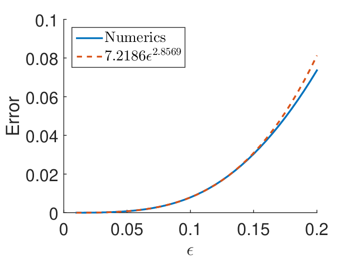
We have performed similar computations for several different values of $\epsilon\to 0$ . Taking $\tau_{0}=1$ , we record sup ${}_{t\in[0,2\tau_{0}/\epsilon]}\lVert y(t)\rVert$ for each $\epsilon$ . We plot in Fig. 1 the maximum error within the time interval as a function of $\epsilon$ . We also plot in the same panel the best power fit in the nonlinear least squares sense, showing that the error is approximately of order $\mathcal{O}(\epsilon^{3/2})$ in agreement with Theorem 1.

4.2 Discrete solitons vs. discrete breathers

Our simulations in Fig. 1 indicate that discrete solitons of the Schrödinger equation shall approximate breathers, i.e., solutions that are periodic in time but localised in space, of the discrete Klein-Gordon equation. Yet, how close are the actual discrete breathers from the solitons? If they are quite close, do they share the same stability characteristics?

To answer the questions, we need to look for breathers of (1). Due to the temporal periodicity of the solutions, we can write $u_{j}(t)$ in trigonometric series:

u_{j}(t)=\sum_{k=1}^{K}a_{j,k}\cos\left(\left(k-1\right)\Omega t\right)+b_{j,k}\sin\left(k\Omega t\right),\,j=1,2,\dots,N,

(33)

where $a_{j,k}$ and $b_{j,k}$ are the Fourier coefficients and $K$ is the number of Fourier modes we will use in our numerics. Herein, we use $K=3$ and $N=50$ , even though larger numbers have been used as well to make sure that the results are independent of the lattice size and the number of modes.

Substituting the series (33) into Eq. (1) and integrating the resulting equation over the time-period $2\pi/\Omega$ , one will obtain coupled nonlinear equations for the coefficients $a_{j,k}$ and $b_{j,k}$ . We then use Newton’s method to solve the resulting equations. Breathers will be obtained by properly choosing the initial guess for the coefficients.

Once a solution, e.g., $\hat{u}_{j}(t)$ , is obtained, we determine its linear stability using Floquet theory. Defining $u_{j}(t)=\hat{u}_{j}(t)+\delta Y_{j}(t),$ substituting it into Eq. (1), and linearising about $\delta=0$ , we obtain the linear second-order differential-difference equation

\begin{array}[]{ccl}\dot{Y}_{j}&=&Z_{j},\\ \dot{Z}_{j}&=&-Y_{j}-3\xi\hat{u}_{j}^{2}Y_{j}+\epsilon\Delta_{2}Y_{j}-\alpha{Z}_{j}.\end{array}

(34)

By integrating the system of linear equations until $t={2\pi}/{\Omega}$ , and using a standard basis in $\mathbb{R}^{2N}$ , i.e., $\left\{e^{0}_{1},e^{0}_{2},...,e^{0}_{2N}\right\}$ as the initial condition at $t=0$ , we obtain a collection of solutions at $t={2\pi}/{\Omega}$ :

M=\left\{E_{1},E_{2},...,E_{2N}\right\}\in\mathbb{R}^{2N\times 2N},

(35)

as a monodromy matrix. The solution $\hat{u}_{j}(t)$ is said to be linearly stable when all the eigenvalues $\lambda$ of the monodromy matrix lies inside or on the unit circle and unstable when there exists at least one $\lambda$ that is outside the unit circle.

As for discrete solitons of the Schrödinger equation (4), after a standing wave solution $\tilde{A}_{j}=(\tilde{x}_{j}+i\tilde{y}_{j})$ is obtained, its linear stability can also be determined from solving the linear eigenvalue problem

\lambda\left(\begin{array}[]{c}\hat{x}_{j}\\ \hat{y}_{j}\end{array}\right)=\left(\begin{array}[]{cc}-6\xi{x}_{j}{y}_{j}-\alpha&\Delta-\omega-3\xi\left({x}_{j}^{2}+3{y}_{j}^{2}\right)\\ \omega-\Delta+3\xi\left(3{x}_{j}^{2}+{y}_{j}^{2}\right)&6\xi{x}_{j}{y}_{j}-\alpha\end{array}\right)\left(\begin{array}[]{c}\hat{x}_{j}\\ \hat{y}_{j}\end{array}\right),

(36)

that is derived straightforwardly as above from substituting $A_{j}=\tilde{A}_{j}+\delta(\hat{x}_{j}+i\hat{y}_{j})e^{\lambda\tau}$ into Eq. (4) and linearising the equation about $\delta=0$ . Solution $\tilde{A}_{j}$ is said to be linearly stable when all of the eigenvalues have Re $(\lambda)\leq 0$ and unstable when there is an eigenvalue with Re $(\lambda)>0$ .

We present in Fig. 2 a breather solution and its time-dynamics in one period for $\epsilon=0.05$ . We also compare in Fig. 2 the breather in panel (a) and the approximation (3) where $A_{j}$ is the discrete soliton solution obtained from solving Eq. (4). One can see the good agreement between them.

By defining the error between breathers of (1) and the approximation (3) using discrete solitons of (4) as

\mathcal{E}=\sup_{0\leq t<2\pi/\Omega}\lVert y(t)\rVert_{\ell^{2}(\mathbb{Z}_{N})},

we plot the error in Fig. 3 for varying $\epsilon$ . We also depict in the same picture, the best power fit, which interestingly shows an algebraic power that follows the estimated error in Theorem 1, i.e., $\sim\epsilon^{3/2}$ .

For the sake of completeness, we show in Fig. 4 the Floquet multipliers of the solution in Fig. 2 for $\epsilon=0.05$ , that are obtained from solving the linear equations (34). Because all the eigenvalues are inside the unit circle, the breather is stable. We plot the eigenvalues of the corresponding discrete soliton in Fig. 4, also showing stability. Because both solutions are stable, the error between them, that is initially of order $\mathcal{O}(\epsilon^{3/2})$ , will stay the same as time evolves until at least $t=2\tau_{0}/\epsilon,$ for some $\tau_{0}>0$ .

When $\epsilon$ is taken to be larger, we observe that breathers of Eq. (1) can become unstable. Shown in Fig. 4 are the Floquet multipliers of the breather when $\epsilon=0.1$ . Because there is an eigenvalue outside the unit circle, the localised solution is unstable. The unstable eigenvalue bifurcates from the collision of an eigenvalue with the continuous spectrum. Note that the corresponding localised solution of the approximating Schrödinger equation (4) is still the same as that shown in Fig. 2, i.e., it is a stable solution.

We show in Fig. 4 the dynamics of the unstable solution. One can observe that it maintains its shape in the form of periodic oscillations for a while, i.e., $t\sim 2\tau_{0}/\epsilon$ . After that, the breather starts to deform and break up. Eventually the solution will collapse, i.e. unbounded blow-up, which is typical for the Klein-Gordon equation (1), even when it is undriven [2] (see also a related work [8]).

Acknowledgements

YM thanks MoRA (Ministry of Religious Affairs) Scholarship of the Republic of Indoesia for a financial support. The research of FTA and BEG are supported by Riset P3MI ITB 2019. RK gratefully acknowledges financial support from Lembaga Pengelolaan Dana Pendidikan (Indonesia Endowment Fund for Education) (Grant No. - Ref: S-34/LPDP.3/2017).

References

[1] F.K. Abdullaev, V.V. Konotop, Nonlinear Waves: Classical and Quantum Aspects, NATO Science Series II: Mathematics, Physics and Chemistry 153 (2005).
[2] V. Achilleos, A. Álvarez, J. Cuevas, D.J. Frantzeskakis, N.I. Karachalios, P.G. Kevrekidis, and B. Sánchez-Rey, Escape dynamics in the discrete repulsive $\phi^{4}$ model, Physica D: Nonlinear Phenomena 244, no. 1 (2013): 1-24.
[3] A. Ali, H. Susanto, and J.A.D. Wattis, Decay of bound states in a sine-Gordon equation with double-well potentials, Journal of Mathematical Physics 56, no. 5 (2015): 051502.
[4] D. Bambusi, S Paleari, and T. Penati, Existence and continuous approximation of small amplitude breathers in 1D and 2D Klein-Gordon lattices, Applicable Analysis 89, no. 9 (2010): 1313-1334.
[5] I.V. Barashenkov, and Y.S. Smirnov, Existence and stability chart for the ac-driven, damped nonlinear Schrödinger solitons, Physical Review E 54, no. 5 (1996): 5707.
[6] O.M.Braun, and Y.S Kivshar, The Frenkel-Kontorova model: concepts, methods, and applications. Springer Science & Business Media, 2004.
[7] I. Daumont, T. Dauxois, and M. Peyrard, Modulational instability: first step towards energy localization in nonlinear lattices, Nonlinearity 10, no. 3 (1997): 617.
[8] J. Diblík, M. Fečkan, M. Pospíšil, V.M. Rothos, and H. Susanto, Travelling waves in nonlinear magnetic metamaterials, In Localized Excitations in Nonlinear Complex Systems, pp. 335-358. Springer, Cham, 2014.
[9] W. Dörfler, A. Lechleiter, M. Plum, G. Schneider, and C. Wieners, Photonic crystals: Mathematical analysis and numerical approximation. Vol. 42, Springer Science & Business Media, 2011.
[10] L.Q. English, F. Palmero, P. Candiani, J. Cuevas, R. Carretero-González, P.G. Kevrekidis, and A.J. Sievers, Generation of localized modes in an electrical lattice using subharmonic driving, Physical review letters 108, no. 8 (2012): 084101.
[11] S. Flach, and C.R. Willis, Discrete breathers, Physics reports 295, no. 5 (1998): 181-264.
[12] M. Johansson, Discrete nonlinear Schrödinger approximation of a mixed Klein–Gordon/Fermi–Pasta–Ulam chain: Modulational instability and a statistical condition for creation of thermodynamic breathers, Physica D: Nonlinear Phenomena 216, no. 1 (2006): 62-70.
[13] E. Kenig, B.A. Malomed, M.C. Cross, and R. Lifshitz, Intrinsic localized modes in parametrically driven arrays of nonlinear resonators, Physical Review E 80, no. 4 (2009): 046202.
[14] P. Kirrmann, G. Schneider, and A. Mielke, The validity of modulation equations for extended systems with cubic nonlinearities, Proceedings of the Royal Society of Edinburgh Section A: Mathematics 122, no. 1-2 (1992): 85-91.
[15] Y.S. Kivshar, Localized modes in a chain with nonlinear on-site potential, Physics Letters A 173, no. 2 (1993): 172-178.
[16] Y.S. Kivshar, and M. Peyrard, Modulational instabilities in discrete lattices, Physical Review A 46, no. 6 (1992): 3198.
[17] P. Kramer, The Method of Multiple Scales for nonlinear Klein-Gordon and Schrödinger Equations, PhD diss., Karlsruhe Institute of Technology, 2013.
[18] R. Lifshitz, and M.C. Cross, Nonlinear dynamics of nanomechanical and micromechanical resonators, Review of nonlinear dynamics and complexity 1 (2008): 1-52.
[19] A.M. Morgante, M. Johansson, G. Kopidakis, and S. Aubry, Standing wave instabilities in a chain of nonlinear coupled oscillators, Physica D: Nonlinear Phenomena 162, no. 1-2 (2002): 53-94
[20] G.M. N’Guérékata, and A. Pankov, Global well-posedness for discrete non-linear Schrödinger equation, Applicable Analysis 89, no. 9 (2010): 1513-1521.
[21] P. Pacciani, V.V. Konotop, and G.P. Menzala, On localized solutions of discrete nonlinear Schrödinger equation: An exact result, Physica D: Nonlinear Phenomena 204, no. 1-2 (2005): 122-133.
[22] D. Pelinovsky, T. Penati, and S. Paleari, Approximation of small-amplitude weakly coupled oscillators by discrete nonlinear Schrödinger equations, Reviews in Mathematical Physics 28, no. 07 (2016): 1650015.
[23] M. Syafwan, H. Susanto, and S.M. Cox, Discrete solitons in electromechanical resonators, Physical Review E 81, no. 2 (2010): 026207.
[24] G. Terrones, D.W. McLaughlin, E.A. Overman, and A.J. Pearlstein, SIAM (Soc. Ind. Appl. Math.) J. Appl. Math. 50, 791 (1990), SIAM (Soc. Ind. Appl. Math.) J. Appl. Math. 50 (1990): 791.