跳到论文正文
W Papers独立论文阅读器 arXiv:1911.01536 论文正文 计算阅读时间 · 0%
引用这篇论文根据当前论文元数据生成,正式投稿前建议核对。


License: arXiv.org perpetual non-exclusive license
arXiv:1911.01536v1 [eess.SY] 04 Nov 2019

Spectral Representations of Graphons in Very Large Network Systems Control

Shuang Gao    Peter E. Caines Thanks: *This work is supported by NSERC (Canada) and the U.S. ARL grant W911NF1910110. Thanks: Shuang Gao and Peter E. Caines are with the Department of Electrical and Computer Engineering, McGill University, Montreal, QC, Canada      ${$sgao,peterc$}$@cim.mcgill.ca.
Abstract

Graphon-based control has recently been proposed and developed to solve control problems for dynamical systems on networks which are very large or growing without bound (see Gao and Caines, CDC 2017, CDC 2018). In this paper, spectral representations, eigenfunctions and approximations of graphons, and their applications to graphon-based control are studied. First, spectral properties of graphons are presented and then approximations based on Fourier approximated eigenfunctions are analyzed. Within this framework, two classes of graphons with simple spectral representations are given. Applications to graphon-based control analysis are next presented; in particular, the controllability of systems distributed over very large networks is expressed in terms of the properties of the corresponding graphon dynamical systems. Moreover, spectral analysis based upon real-world network data is presented, which demonstrates that low-dimensional spectral approximations of networks are possible. Finally, an initial, exploratory investigation of the utility of the spectral analysis methodology in graphon systems control to study the control of epidemic spread is presented.

I Introduction

Graphon theory has been developed to study large networks and graph limits [1, 2, 3]. Recently it has been applied to study dynamical systems such as the heat equation [4], coupled oscillators [5] and power network synchronization [6], to analyze network centrality [7], to investigate static and dynamic games [8, 9], and to control large networks of dynamical systems [10, 11, 12, 13, 9]. Graphon theory provides a theoretical tool for the study of arbitrarily large and, in the limit, infinite network systems, and thus enables low-complexity approximate solutions to control problems on such systems [10, 11, 12, 13, 9].

Among these applications, graphon spectral properties are very significant [14]. In fact, the spectral analysis of large-scale systems has been studied since the late 1960s [15] and it plays a key role to the low-complexity control synthesis of such systems [16, 17, 15]. This leads us to the study of spectral representations and approximations of graphons in this paper.

As operators, graphons are Hilbert-Schmidt integral operators and hence are compact. Moreover, the symmetry property of graphons ensures that the Spectral Theorem [18] applies to graphon operators. Topics on Hilbert-Schmidt integral operators and self-adjoint compact operators have been extensively studied in the literature (see e.g. [19, 20, 18]), and the spectral properties of graphons, for instance, are investigated in [21].

This paper studies the control and analysis of graphon systems and their associated networks via the exploitation of their spectral properties. The contributions of this paper include 1) the presentation of the spectral representations of two types of graphons, 2) an analysis of the exact controllability of a class of graphon dynamical systems based on spectral decompositions, 3) the study of network spectral properties based on real-world network data which demonstrates that low-dimensional spectral approximations of networks are possible, and 4) the initial, exploratory investigation of the utility of the spectral analysis methodology in graphon systems control to study the controlled epidemic spread process

Notation

ℝ\mathds{R}, ℝ+\mathds{R}_{+} and ℤ+\mathds{Z}_{+} represent respectively the sets of all real numbers, all positive real numbers and all positive integers. ⟨⋅,⋅⟩\langle\cdot,\cdot\rangle and ∥⋅∥\|\cdot\| denote respectively inner product and norm. Bold face letters (e.g. 𝐀\mathbf{A}, 𝐁\mathbf{B}, 𝐮\mathbf{u}) are used to represent graphons and functions. Blackboard bold letters (e.g. 𝕀\mathbb{I}, 𝔸\mathbb{A}, 𝔹\mathbb{B}, 𝕎\mathbb{W}) are used to denote linear operators which are not necessarily compact; in particular, 𝕀\mathbb{I} denotes the identity operator.

II Graphs and Graphons

Network structures can be modeled as graphs. A graph G=(V,E)G=(V,E) is specified by an node set VV and an edge set E⊂V×VE\subset V\times V. It has a representation by the corresponding adjacency matrix A=[ai​j]A=[a_{ij}] where the element ai​ja_{ij} is one when there is an edge from node ii to node jj, and zero otherwise. For a weighted graph, the elements of its adjacency matrix represent the corresponding edge weights. Furthermore, if one embeds the adjacency matrix on [0,1]2[0,1]^{2} as a pixel picture where each pixel has a side length 1|V|\frac{1}{|V|} with |V||V| representing the cardinality of VV, then it gives a function 𝐀:[0,1]2→[0,1]\mathbf{A}:[0,1]^{2}\rightarrow[0,1].

Formally, graphons are defined as bounded symmetric Lebesgue measurable functions 𝐀:[0,1]2→[0,1]\mathbf{A}:[0,1]^{2}\rightarrow[0,1], which can be interpreted as weighted graphs on the node set [0,1][0,1]. A meaningful convergence with respect to the cut metric (see e.g. [3]) is defined for sequences of dense and finite graphs. Graphons are then the limit objects of converging graph sequences. Moreover, graphons can be used as generative models for exchangeable random graphs [22]. These properties make graphons suitable to model extremely large-scale networks. We note that in some papers, for instance [23], the word “graphon” refers to symmetric, integrable functions from [0,1]2[0,1]^{2} to ℝ\mathds{R}. In this paper, unless stated otherwise, the term “graphon” refers to a bounded symmetric Lebesgue measurable function 𝐀1:[0,1]2→[−1,1]{\mathbf{A}_{1}}:[0,1]^{2}\rightarrow[-1,1], so as to include networks with possibly negative weights, and 𝒲1\mathcal{W}_{1} denotes the set of all graphons. Let 𝒲0\mathcal{W}_{0} represent the set of all graphons satisfying 𝐀0:[0,1]2→[0,1]{\mathbf{A}_{0}}:[0,1]^{2}\rightarrow[0,1]. 𝒲0\mathcal{W}_{0} and 𝒲1\mathcal{W}_{1} are both compact under the cut metric (after identifying points of zero distance) [3].

III Graphon Operators

III-A Graphon Operators

Let L2​(Ω)L^{2}(\Omega) be the standard Lebesgue space defined on Ω\Omega endowed with the 22-norm ‖x‖2=(∫Ωx​(α)2​𝑑α)12\|x\|_{2}=({\int_{\Omega}x(\alpha)^{2}d\alpha})^{\frac{1}{2}}. L2​[0,1]L^{2}[0,1] and L2​[0,1]2L^{2}[0,1]^{2} are defined by specializing Ω\Omega to be [0,1][0,1] and [0,1]2[0,1]^{2}, respectively.

Definition 1

A linear map 𝕋:L2​[0,1]→L2​[0,1]\mathbb{T}:L^{2}[0,1]\rightarrow L^{2}[0,1] is said to be compact if 𝕋\mathbb{T} maps the open unit ball in L2​[0,1]L^{2}[0,1] to a set in L2​[0,1]L^{2}[0,1] that has compact closure.

□

Definition 2 ([3])

A graphon operator 𝕋𝐀:L2​[0,1]→L2​[0,1]\mathbb{T}_{\mathbf{A}}:L^{2}[0,1]\rightarrow L^{2}[0,1] is defined by a graphon 𝐀∈𝒲1\mathbf{A}\in\mathcal{W}_{1} as follows:

[𝕋𝐀​𝐟]​(x)=∫01𝐀⁡(x,y)​𝐟​(y)​𝑑y,𝐟⁡(⋅)∈L2​[0,1].[\mathbb{T}_{\mathbf{A}}\mathbf{f}](x)=\int_{0}^{1}\mathbf{A}(x,y)\mathbf{f}(y)dy,\quad\mathbf{f}(\cdot)\in L^{2}[0,1]. (1)

□

Clearly, the operator 𝕋𝐀\mathbb{T}_{\mathbf{A}} is Hermitian (or self-adjoint), since for any x,yx,y in L2​[0,1]L^{2}[0,1], ⟨x,𝕋𝐀​y⟩=⟨𝕋𝐀​x,y⟩\langle x,\mathbb{T}_{\mathbf{A}}y\rangle=\langle\mathbb{T}_{\mathbf{A}}x,y\rangle. Moreover, the graphon operator 𝕋𝐀\mathbb{T}_{\mathbf{A}} is a linear operator that is bounded, (hence) continuous, and compact [24].

For simplicity of notation we henceforth use the bold face letter (e.g. 𝐀\mathbf{A}, 𝐁\mathbf{B}) to represent both a graphon and its corresponding graphon operator. Let 𝐀𝐟\mathbf{A}\mathbf{f} denote the function defined by (1).

The graphon operator product is then defined by

[𝐀𝐁]​(x,y)=∫01𝐀⁡(x,z)​𝐁​(z,y)​𝑑z,[{\mathbf{A}\mathbf{B}}](x,y)=\int_{0}^{1}\mathbf{A}(x,z)\mathbf{B}(z,y)dz, (2)

where 𝐀,𝐁∈𝒲1.{\mathbf{A},\mathbf{B}}\in\mathcal{W}_{1}. Let 𝐀𝐁\mathbf{A}\mathbf{B} denote the graphon given by the convolution in (2). Consequently, the power 𝐀n{\mathbf{A}}^{n} of an operator 𝐀∈𝒲1{\mathbf{A}}\in\mathcal{W}_{1} is given by

𝐀n(x,y)=∫[0,1]n𝐀(x,α1)⋯𝐀(αn−1,y)dα1⋯dαn−1{\mathbf{A}}^{n}(x,y)=\int_{[0,1]^{n}}{\mathbf{A}}(x,\alpha_{1})\cdots{\mathbf{A}}(\alpha_{n-1},y)d\alpha_{1}\cdots d\alpha_{n-1}

with 𝐀n∈𝒲1,n∈ℤ+{\mathbf{A}}^{n}\in\mathcal{W}_{1},n\in\mathds{Z}_{+}. 𝐀0{\mathbf{A}^{0}} is formally defined as the identity operator 𝕀\mathbb{I} on functions in L2​[0,1]L^{2}{[0,1]}, and hence 𝐀0{\mathbf{A}^{0}} is neither a graphon nor a compact operator. Furthermore, e𝐀:=∑k=0∞1k!​𝐀ke^{\mathbf{A}}:=\sum_{k=0}^{\infty}\frac{1}{k!}\mathbf{A}^{k} of a graphon operator 𝐀\mathbf{A} is a bounded linear operator from L2​[0,1]L^{2}[0,1] to L2​[0,1]L^{2}[0,1].

III-B Spectral Representations

Denote the operator norm for a linear operator 𝕋\mathbb{T} on L2​[0,1]L^{2}[0,1] as

‖𝕋‖op=sup𝐟∈L2​[0,1],‖𝐟‖2=1‖𝕋​𝐟‖2.\|\mathbb{T}\|_{\text{{op}}}=\sup_{\mathbf{f}\in L^{2}[0,1],\|\mathbf{f}\|_{2}=1}\|\mathbb{T}\mathbf{f}\|_{2}. (3)

Following [19], we define kernel space, spectrum, eigenvalue and eigenfunction below.

Definition 3

Define the kernel space (or null space) for a linear operator 𝕋\mathbb{T} on L2​[0,1]L^{2}[0,1] as :

Ker​(𝕋):={x∈L2​[0,1]:𝕋​x=0}.\text{Ker}(\mathbb{T}):=\{x\in L^{2}[0,1]:\mathbb{T}x=0\}.

□

Definition 4

The spectrum σ⁡(𝕋)\sigma(\mathbb{T}) of a linear bounded operator 𝕋\mathbb{T} on L2​[0,1]L^{2}[0,1] is the set of all (complex or real) scalars λ\lambda such that 𝕋−λ​𝕀\mathbb{T}-\lambda\mathbb{I} is not invertible, where 𝕀\mathbb{I} is the identity operator. Thus λ∈σ⁡(𝕋)\lambda\in\sigma(\mathbb{T}) if and only if at least one of the following two statements is true:

  1. (i)

    The range of 𝕋−λ​𝕀\mathbb{T}-\lambda\mathbb{I} is not all of L2​[0,1]L^{2}[0,1], i.e., 𝕋−λ​𝕀\mathbb{T}-\lambda\mathbb{I} is not onto.

  2. (ii)

    𝕋−λ​𝕀\mathbb{T}-\lambda\mathbb{I} is not one-to-one.

If (ii) holds, λ\lambda is said to be an eigenvalue of 𝕋\mathbb{T}; the corresponding eigenspace is Ker​(𝕋−λ​𝕀)\text{Ker}(\mathbb{T}-\lambda\mathbb{I}); each x∈Ker​(𝕋−λ​𝕀)x\in\text{Ker}(\mathbb{T}-\lambda\mathbb{I}) (except x=0x=0) is an eigenfunction of 𝕋\mathbb{T}; it satisfies the equation 𝕋​x=λ​x\mathbb{T}x=\lambda x. □

Lemma 1 ([12])

For any graphon 𝐀\mathbf{A} or any function 𝐀\mathbf{A} in L2​[0,1]2L^{2}[0,1]^{2},

‖𝐀‖op≤‖𝐀‖2,\|\mathbf{A}\|_{\text{{op}}}\leq\|\mathbf{A}\|_{2},

where ‖𝐀‖2=(∫01∫01(𝐀⁡(x,y))2​𝑑x​𝑑y)12\|\mathbf{A}\|_{2}=\big(\int_{0}^{1}\int_{0}^{1}(\mathbf{A}(x,y))^{2}dxdy\big)^{\frac{1}{2}}. □

Hence a graphon sequence convergences under ∥⋅∥2\|\cdot\|_{2} implies it convergences under ∥⋅∥op\|\cdot\|_{\text{{op}}}. Furthermore, the following inequalities hold [25, 8]:

‖𝐀‖□≤‖𝐀‖op≤8​‖𝐀‖□,\|\mathbf{A}\|_{\Box}\leq\|\mathbf{A}\|_{\text{\text{{op}}}}\leq\sqrt{8\|\mathbf{A}\|_{\Box}}, (4)

where the cut norm of a graphon 𝐀∈𝒲1\mathbf{A}\in\mathcal{W}_{1} is defined as

‖𝐀‖□=supM,T⊂[0,1]|∫M×T𝐀⁡(x,y)​𝑑x​𝑑y|.\|\mathbf{A}\|_{\Box}=\sup_{M,T\subset[0,1]}|\int_{M\times T}\mathbf{A}(x,y)dxdy|. (5)

The cut metric between two graphons 𝐕\mathbf{V} and 𝐖\mathbf{W} is then given by

δ□​(𝐖,𝐕)=infϕ∈S[0,1]‖𝐖ϕ−𝐕‖□,\delta_{\Box}(\mathbf{W,V})=\inf_{\phi\in S_{[0,1]}}\|\mathbf{W}^{\phi}-\mathbf{V}\|_{\Box}, (6)

where 𝐖ϕ​(x,y)=𝐖⁡(ϕ⁡(x),ϕ⁡(y))\mathbf{W}^{\phi}(x,y)=\mathbf{W}(\phi(x),\phi(y)) and S[0,1]S_{[0,1]} denotes the set of measure preserving bijections from [0,1][0,1] to [0,1][0,1]. See [3, 25] for more details on different norms.

Proposition 1

Consider the graphon operator 𝐀\mathbf{A} corresponding to a graphon 𝐀∈𝒲1\mathbf{A}\in\mathcal{W}_{1}. Then there is a set {𝐟ℓ}\{\mathbf{f}_{\ell}\} consisting of a countable number of orthonormal elements in L2​[0,1]L^{2}[0,1] such that the elements 𝐟ℓ\mathbf{f}_{\ell} are eigenfunctions to the eigenvalues λℓ∈ℝ\lambda_{\ell}\in\mathds{R} ordered as follows:

‖𝐀‖op=|λ1|≥|λ2|≥|λ3|≥…≥0,\|\mathbf{A}\|_{\text{{op}}}=|\lambda_{1}|\geq|\lambda_{2}|\geq|\lambda_{3}|\geq...\geq 0,

If the set {𝐟ℓ}\{\mathbf{f}_{\ell}\} is infinite, we have the asymptotic behavior limℓ→∞λℓ=0.\lim_{\ell\rightarrow\infty}\lambda_{\ell}=0. Furthermore, for any 𝐮∈L2​[0,1]\mathbf{u}\in L^{2}[0,1], 𝐀𝐮\mathbf{A}\mathbf{u} has representations as:

𝐀𝐮=∑ℓ=1∞λℓ​⟨𝐟ℓ,𝐮⟩​𝐟ℓ​ and ​⟨𝐮,𝐀𝐮⟩=∑ℓ=1∞λℓ​|⟨𝐟ℓ,𝐮⟩|2.\mathbf{A}\mathbf{u}=\sum_{\ell=1}^{\infty}\lambda_{\ell}\langle\mathbf{f}_{\ell},\mathbf{u}\rangle\mathbf{f}_{\ell}\text{ and }\langle\mathbf{u},\mathbf{A}\mathbf{u}\rangle=\sum_{\ell=1}^{\infty}\lambda_{\ell}|\langle\mathbf{f}_{\ell},\mathbf{u}\rangle|^{2}.

□

This result is a special case of [18, Theorem 7.3], where the compact Hermitian operators there are specialized to graphon operators.

III-C Convergence of Eigenvalues

For a graphon 𝐀\mathbf{A}, the eigenvalues form two sequences μ1​(𝐀)≥μ2​(𝐀)≥…≥0\mu_{1}(\mathbf{A})\geq\mu_{2}(\mathbf{A})\geq...\geq 0 and μ1′​(𝐀)≤μ2′​(𝐀)≤…≤0\mu^{\prime}_{1}(\mathbf{A})\leq\mu^{\prime}_{2}(\mathbf{A})\leq...\leq 0 converging to zero, where μi​(𝐀)\mu_{i}{(\mathbf{A})} and μi′​(𝐀)\mu_{i}^{\prime}{(\mathbf{A})} denote respectively the it​hi^{th} non-negative eigenvalue and the it​hi^{th} non-positive eigenvalue.

Theorem 1 ([2])

Let {𝐀i}i=1∞\{\mathbf{A}_{i}\}_{i=1}^{\infty} be a sequence of uniformly bounded graphons, converging in the cut metric to a graphon 𝐀\mathbf{A}. Then for every i≥1i\geq 1,

μi​(𝐀n)→μi​(𝐀)andμi′​(𝐀n)→μi′​(𝐀) as ​n→∞.\mu_{i}(\mathbf{A}_{n})\rightarrow\mu_{i}(\mathbf{A})\quad\text{and}\quad{\mu}^{\prime}_{i}(\mathbf{A}_{n})\rightarrow{\mu}^{\prime}_{i}(\mathbf{A})\quad\text{ as }n\rightarrow\infty.

□

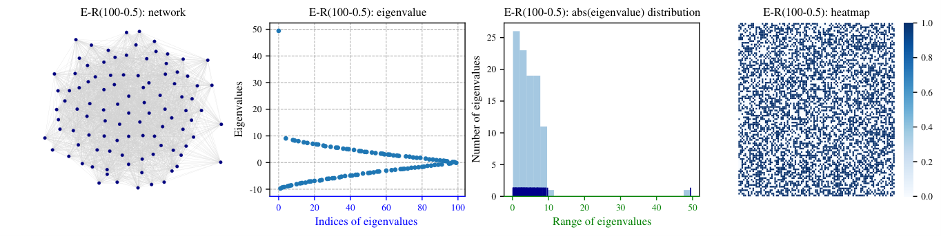
This implies that if a sequence of graphs converges in the cut metric [3] to a graphon limit with a simple spectral characterization by a few non-zero eigenvalues, then the sequence of graphs admits simple low-dimensional spectral approximations. Furthermore, if the graphs in the sequence are increasing in size, then the low-dimensional approximations perform better as the networks increase in size. This can be illustrated by the sequence of random graphs generated by the Erdös-Rényi model in Fig. 1. For general random graphs generated by dense low-rank models, reasonable low-rank approximations exist [26].
Refer to caption
Fig. 1: The eigenvalue distribution of a graph with 100 nodes in a convergent sequence of random graphs to the graphon limit W⁡(x,y)=0.5W(x,y)=0.5. Notice that the eigenvalues accumulate at 00 and 0.5×1000.5\times 100 which correspond to the eigenvalues of the graphon W⁡(x,y)=0.5W(x,y)=0.5. This feature makes it possible to approximate certain large random networks by low dimensional spectral characterizations.

IV Approximation of Graphons

If the eigenvalues and the corresponding eigenfunctions of a graphon are known, one can approximate the graphon by a finite spectral sum. Consider the approximation of a graphon 𝐀\mathbf{A} by 𝐀m​(x,y)=∑ℓ=1mλℓ​𝐟ℓ​(x)​𝐟ℓ​(y)\mathbf{A}_{m}(x,y)=\sum_{\ell=1}^{m}\lambda_{\ell}\mathbf{f}_{\ell}(x)\mathbf{f}_{\ell}(y). Then the mean square error is given as follows:

‖𝐀−𝐀m‖2=‖𝐀‖22−∑ℓ=1mλℓ2.\displaystyle\|\mathbf{A}-\mathbf{A}_{m}\|_{2}=\sqrt{\|\mathbf{A}\|_{2}^{2}-\sum_{\ell=1}^{m}\lambda_{\ell}^{2}}. (7)

Denote pℓ​(⋅)p_{\ell}(\cdot) as a polynomial function and pℓ(e2πi⋅)p_{\ell}(e^{2\pi i\cdot}) is used to approximate the ℓt​h\ell^{th} eigenfunction 𝐟ℓ​(⋅)\mathbf{f}_{\ell}(\cdot) of 𝐀\mathbf{A} with 𝐀⁡(x,y)=∑ℓ=1∞λℓ​𝐟ℓ​(x)​𝐟ℓ​(y)\mathbf{A}(x,y)=\sum_{\ell=1}^{\infty}\lambda_{\ell}\mathbf{f}_{\ell}(x)\mathbf{f}_{\ell}(y). Note that if the polynomial pℓ​(⋅)p_{\ell}(\cdot) permits terms up to infinite order, pℓ(e2πi⋅)p_{\ell}(e^{2\pi i\cdot}) is simply the Fourier representation of 𝐟ℓ​(⋅)\mathbf{f}_{\ell}(\cdot). Denote the spectral sum with Fourier approximated eigenfunctions as

𝐀p​m​(ϑ,ψ)=∑ℓ=1mλℓ​pℓ​(e2​π​i​ϑ)​pℓ​(e2​π​i​ψ)\mathbf{A}_{pm}(\vartheta,\psi)=\sum_{\ell=1}^{m}\lambda_{\ell}p_{\ell}(e^{2\pi i\vartheta})p_{\ell}(e^{2\pi i\psi}) (8)

There are two levels of approximations: (a) Fourier approximation of eigenfunctions; (b) spectral decomposition approximation of the graphon operator. Hence the approximation error is bounded as follows:

‖𝐀−𝐀p​m‖2≤‖𝐀−𝐀m‖2+‖𝐀m−𝐀p​m‖2.\|\mathbf{A}-\mathbf{A}_{pm}\|_{2}\leq\|\mathbf{A}-\mathbf{A}_{m}\|_{2}+\|\mathbf{A}_{m}-\mathbf{A}_{pm}\|_{2}.

Moreover, the approximation error for functions of operators is given in the following.

Proposition 2 ([13])

If there exists c>0c>0 such that ‖𝐀‖2≤c\|\mathbf{A}\|_{2}\leq c and ‖𝐀p​m‖2≤c\|\mathbf{A}_{pm}\|_{2}\leq c, then

‖𝐀n−(𝐀p​m)n‖2≤n​cn​‖𝐀−𝐀p​m‖2,\displaystyle\|\mathbf{A}^{n}-(\mathbf{A}_{pm})^{n}\|_{2}\leq nc^{n}\|\mathbf{A}-\mathbf{A}_{pm}\|_{2}, (9)
‖e𝐀−e𝐀p​m‖op≤c​ec​‖𝐀−𝐀p​m‖2.\displaystyle\|e^{\mathbf{A}}-e^{\mathbf{A}_{pm}}\|_{\text{{op}}}\leq ce^{c}\|\mathbf{A}-\mathbf{A}_{pm}\|_{2}. (10)

□

Consider a polynomial pℓ(e2πi⋅)p_{\ell}(e^{2\pi i\cdot}) with highest order 2​n2n, then there exists a matrix Tℓ∈ℝn×nT_{\ell}\in\mathds{R}^{n\times n} such that

pℓ(e2πi⋅)=(e1,e2,…en)Tℓ(e1,e2,…en)Tp_{\ell}(e^{2\pi i\cdot})=(e_{1},e_{2},...e_{n})T_{\ell}(e_{1},e_{2},...e_{n})^{T}

with ek=e2πki⋅e_{k}=e^{2\pi ki\cdot}. Since Fourier basis forms a complete basis for L2​[0,1]L^{2}[0,1] (see e.g. [27]), any function 𝐟∈L2​[0,1]\mathbf{f}\in L^{2}[0,1] can be approximated by finite Fourier series and hence by polynomial functions of e2πi⋅e^{2\pi i\cdot}.

V Graphons with Simple Spectral Representations

V-A Sinusoidal Graphons

A sinusoidal graphon is defined as any graphon that can be represented by

𝐀⁡(φ,ϑ)=a0+∑k=1∞bk​cos⁡(2​π​k​(φ−ϑ)),(φ,ϑ)∈[0,1]2.\mathbf{A}(\varphi,\vartheta)=a_{0}+\sum_{k=1}^{\infty}b_{k}\cos(2\pi k(\varphi-\vartheta)),\quad(\varphi,\vartheta)\in[0,1]^{2}. (11)

Clearly sinusoidal graphons are symmetric and diagonally constant and hence they are suitable to fit Toeplitz matrices [28].

Sinusoidal graphons have simple spectral characterizations. The eigenfunctions of the graphon in (11) are L2​[0,1]L^{2}[0,1] functions as follows:

1,{2​cos⁡2​π​k​(⋅):k∈ℤ+},{2​sin⁡2​π​k​(⋅):k∈ℤ+}.1,\{\sqrt{2}\cos 2\pi k(\cdot):k\in\mathds{Z}_{+}\},\{\sqrt{2}\sin 2\pi k(\cdot):k\in\mathds{Z}_{+}\}.

The corresponding eigenvalues are: a0,{bk2:k∈ℤ+},{bk2:k∈ℤ+}.a_{0},\{\frac{b_{k}}{2}:k\in\mathds{Z}_{+}\},\{\frac{b_{k}}{2}:k\in\mathds{Z}_{+}\}. Moreover, the eigenfunctions form a complete orthonormal basis for L2​[0,1]L^{2}[0,1] (see [27]).

V-A1 Operation on L2​[0,1]L^{2}[0,1] functions

Consider a function 𝐱∈L2​[0,1]\mathbf{x}\in L^{2}[0,1] represented by Fourier series as

𝐱⁡(ϑ)=K0+∑k=1∞(αk​sin⁡(ϑ)+βk​cos⁡(ϑ)),ϑ∈[0,1].\mathbf{x}({\vartheta})=K_{0}+\sum_{k=1}^{\infty}(\alpha_{k}\sin(\vartheta)+\beta_{k}\cos(\vartheta)),\quad\vartheta\in[0,1].

Then operating a sinusoidal graphon 𝐀\mathbf{A} on 𝐱\mathbf{x} yields

[𝐀𝐱]​(ϑ)=a0​K0+∑k=1∞bk2​(αk​sin⁡(ϑ)+βk​cos⁡(ϑ)),ϑ∈[0,1].[\mathbf{A}\mathbf{x}](\vartheta)=a_{0}K_{0}+\sum_{k=1}^{\infty}\frac{b_{k}}{2}(\alpha_{k}\sin(\vartheta)+\beta_{k}\cos(\vartheta)),~\vartheta\in[0,1].

Similarly, for m∈ℤ+m\in\mathds{Z}_{+} and ϑ∈[0,1],\vartheta\in[0,1],

[𝐀m​𝐱]​(ϑ)=a0m​K0+∑k=1∞(bk2)m​(αk​sin⁡(ϑ)+βk​cos⁡(ϑ)),\displaystyle[\mathbf{A}^{m}\mathbf{x}](\vartheta)=a_{0}^{m}K_{0}+\sum_{k=1}^{\infty}\left(\frac{b_{k}}{2}\right)^{m}(\alpha_{k}\sin(\vartheta)+\beta_{k}\cos(\vartheta)),
[e𝐀​𝐱]​(ϑ)=ea0​K0+∑k=1∞ebk2​(αk​sin⁡(ϑ)+βk​cos⁡(ϑ)).\displaystyle[e^{\mathbf{A}}\mathbf{x}](\vartheta)=e^{a_{0}}K_{0}+\sum_{k=1}^{\infty}e^{\frac{b_{k}}{2}}(\alpha_{k}\sin(\vartheta)+\beta_{k}\cos(\vartheta)).

V-A2 Functions of sinusoidal graphons

Power functions of a sinusoidal graphon 𝐀\mathbf{A} are given by

𝐀m​(φ,ϑ)=a0m+∑k=1∞(bk2)m−1⋅bk​cos⁡(2​π​k​(φ−ϑ)),\displaystyle\mathbf{A}^{m}(\varphi,\vartheta)=a_{0}^{m}+\sum_{k=1}^{\infty}(\frac{b_{k}}{2})^{m-1}\cdot b_{k}\cos(2\pi k(\varphi-\vartheta)),

where (φ,ϑ)∈[0,1]2,m∈ℤ+(\varphi,\vartheta)\in[0,1]^{2},m\in\mathds{Z}_{+}. Moreover, the time-varying exponential function of a sinusoidal graphon is given by e𝐀​t=𝕀+𝐔t,t∈ℝ,e^{\mathbf{A}t}=\mathbb{I}+{\mathbf{U}}_{t},~t\in\mathds{R}, where 𝐔t\mathbf{U}_{t} is defined as follows: for all (φ,ϑ)∈[0,1]2(\varphi,\vartheta)\in[0,1]^{2}

𝐔t​(φ,ϑ)=(ea0​t−1)+2​∑k=1∞(ebk2​t−1)​cos⁡2​π​k​(φ−ϑ).\begin{split}&\mathbf{U}_{t}(\varphi,\vartheta)=\left(e^{a_{0}t}-1\right)+2\sum_{k=1}^{\infty}\left(e^{\frac{b_{k}}{2}t}-1\right)\cos 2\pi k(\varphi-\vartheta).\\ \end{split}

We note that, for any t∈ℝ,t\in\mathds{R}, e𝐀​te^{\mathbf{A}t} is an element of the graphon unitary operator algebra [11].

V-B Step Function Graphons

A graphon 𝐀∈𝒲1{\mathbf{A}}\in\mathcal{W}_{1} is a step function if there is a partition Q={Q1,…,QN}Q=\{Q_{1},...,Q_{N}\} of [0,1][0,1] into measurable sets such that 𝐀{\mathbf{A}} is constant on every product set Qi×QjQ_{i}\times Q_{j}. A uniform partition PN={P1,P2,…,PN}P^{N}=\{P_{1},P_{2},...,P_{N}\} of [0,1][0,1] is given by setting Pk=[k−1N,kN),k∈{1,N−1}P_{k}=[\frac{k-1}{N},\frac{k}{N}),k\in\{1,N-1\} and PN=[N−1N,1]P_{N}=[\frac{N-1}{N},1]. In this paper, we focus on step functions with uniform partitions. For general step functions, see [3].

The piece-wise constant function 𝕊u\mathds{S}_{u} in L2​[0,1]L^{2}[0,1] corresponding to u∈ℝNu\in\mathds{R}^{N} is defined as

𝕊u(x)=∑i=1N𝟙Pi(x)ui,∀x∈[0,1]\mathds{S}_{u}(x)=\sum_{i=1}^{N}{\mathds{1}}_{{}_{P_{i}}}(x)u_{i},\quad\forall x\in[0,1] (12)

where 𝟙Pi(⋅)\mathds{1}_{{}_{P_{i}}}(\cdot) denotes the indicator function, that is, 𝟙Pi(x)=1\mathds{1}_{{}_{P_{i}}}(x)=1 if x∈Pix\in P_{i} and 𝟙Pi(x)=0\mathds{1}_{{}_{P_{i}}}(x)=0 if x∉Pix\notin P_{i}. Let 𝕊u⋅𝕊vT\mathds{S}_{u}\cdot\mathds{S}_{v}^{T} be given as follows:

(x,y)\displaystyle(x,y) :=∑i=1N𝟙Pi(x)ui∑i=1N𝟙Pj(y)vj\displaystyle:=\sum_{i=1}^{N}{\mathds{1}}_{{}_{P_{i}}}(x)u_{i}\sum_{i=1}^{N}{\mathds{1}}_{{}_{P_{j}}}(y)v_{j} (13)

where 𝕊u\mathds{S}_{u} and 𝕊vT\mathds{S}_{v}^{T} share the same uniform partition PN={P1,…,PN}P^{N}=\{P_{1},...,P_{N}\}.

Proposition 3

If the matrix A=[ai​j]A=[a_{ij}] has a spectral decomposition A=V​Λd​V⊺A=V\Lambda_{d}V^{\mathchoice{\raisebox{0.0pt}{$\displaystyle\intercal$}}{\raisebox{0.0pt}{$\textstyle\intercal$}}{\raisebox{0.0pt}{$\scriptstyle\intercal$}}{\raisebox{0.0pt}{$\scriptscriptstyle\intercal$}}}, where Λd=diag​(λ1,…,λd)\Lambda_{d}=\text{diag}(\lambda_{1},...,\lambda_{d}) and V=(v1,….,vd)V=(v_{1},....,v_{d}) with vℓv_{\ell} representing the normalized eigenvector of λℓ\lambda_{\ell}, then the step function graphon 𝐀\mathbf{A} defined by

𝐀(x,y)=∑i=1N∑j=1N𝟙Pi(x)𝟙Pj(y)ai​j,(x,y)∈[0,1]2\mathbf{A}(x,y)=\sum_{i=1}^{N}\sum_{j=1}^{N}\mathds{1}_{{}_{P_{i}}}(x)\mathds{1}_{{}_{P_{j}}}(y)a_{ij},~~(x,y)\in[0,1]^{2} (14)

has a spectral representation given by

𝐀⁡(x,y)\displaystyle\mathbf{A}(x,y) =∑ℓ=1dλℓ[𝕊vℓ⋅𝕊vℓ⊺](x,y),(x,y)∈[0,1]2,\displaystyle=\sum_{\ell=1}^{d}\lambda_{\ell}[\mathds{S}_{v_{\ell}}\cdot\mathds{S}_{v_{\ell}}^{\mathchoice{\raisebox{0.0pt}{$\displaystyle\intercal$}}{\raisebox{0.0pt}{$\textstyle\intercal$}}{\raisebox{0.0pt}{$\scriptstyle\intercal$}}{\raisebox{0.0pt}{$\scriptscriptstyle\intercal$}}}](x,y),~~(x,y)\in[0,1]^{2}, (15)

where the underlying partition {P1,…,PN}\{P_{1},...,P_{N}\} of [0,1][0,1] is uniform. □

Proof

For all (x,y)∈[0,1]2(x,y)\in[0,1]^{2},

𝐀⁡(x,y)\displaystyle\mathbf{A}(x,y) =∑i=1N∑j=1N𝟙Pi(x)𝟙Pi(y)∑ℓ=1dλℓvl(i)vl(j)\displaystyle=\sum_{i=1}^{N}\sum_{j=1}^{N}\mathds{1}_{{}_{P_{i}}}(x)\mathds{1}_{{}_{P_{i}}}(y)\sum_{\ell=1}^{d}\lambda_{\ell}v_{l}(i)v_{l}(j)
=∑ℓ=1dλℓ∑i=1N𝟙Pi(x)vℓ(i)∑j=1N𝟙Pj(y)vℓ(j)\displaystyle=\sum_{\ell=1}^{d}\lambda_{\ell}\sum_{i=1}^{N}\mathds{1}_{{}_{P_{i}}}(x)v_{\ell}(i)\sum_{j=1}^{N}\mathds{1}_{{}_{P_{j}}}(y)v_{\ell}(j)
=∑ℓ=1dλℓ​[𝕊vℓ⋅𝕊vℓT]​(x,y),\displaystyle=\sum_{\ell=1}^{d}\lambda_{\ell}[\mathds{S}_{v_{\ell}}\cdot\mathds{S}_{v_{\ell}}^{T}](x,y),

where vℓ​(i)v_{\ell}(i) denotes the it​hi^{th} element of vℓv_{\ell}. ■

We note that ⟨𝕊vℓ,𝕊vk⟩=0, if ​ℓ≠k;⟨𝕊vℓ,𝕊vk⟩=1N, if ​ℓ=k\langle\mathds{S}_{v_{\ell}},\mathds{S}_{v_{k}}\rangle=0,\text{ if }\ell\neq k;~\langle\mathds{S}_{v_{\ell}},\mathds{S}_{v_{k}}\rangle=\frac{1}{N},\text{ if }\ell=k and hence the corresponding eigenvalues for 𝐀\mathbf{A} are given by {1N​λℓ}ℓ=1d\{\frac{1}{N}\lambda_{\ell}\}_{\ell=1}^{d}.

Piece-wise constant functions in L2​[0,1]L^{2}[0,1] form eigenfunctions of step function graphons. Since piece-wise constant functions in L2​[0,1]L^{2}[0,1] form a dense subset of L2​[0,1]L^{2}[0,1] space, they can also be used to approximate eigenfunctions of general graphons.

VI Graphon Dynamical Systems

Consider a group of linear dynamical subsystems {SiN;1≤i≤N}\{S_{i}^{N};1\leq i\leq N\} coupled over an undirected graph GNG_{N}. The subsystem SiNS_{i}^{N} at the node ii of GNG_{N} has interactions with SjN,1≤j≤N,S_{j}^{N},1\leq j\leq N, specified as below:

x˙it=α0xti+1N∑j=1Nai​jxjt+β0uti+1N∑j=1Nbi​jujt,\displaystyle\dot{x}^{i}_{t}=\alpha_{0}x_{t}^{i}+\frac{1}{N}\sum_{j=1}^{N}{a}_{ij}x^{j}_{t}+\beta_{0}u_{t}^{i}+\frac{1}{N}\sum_{j=1}^{N}{b}{{}_{ij}}u^{j}_{t},\quad (16)
t∈[0,T],α0,β0∈ℝ,xti,uti∈ℝ,\displaystyle t\in[0,T],\quad\alpha_{0},\beta_{0}\in\mathds{R},\quad x^{i}_{t},u^{i}_{t}\in\mathds{R},

with AN=[ai​j]{A}_{N}=[{a}_{ij}] and BN=[bi​j]∈ℝN×N{B}_{N}=[{b}_{ij}]\in\mathds{R}^{N\times N} as the symmetric adjacency matrices of GNG_{N} and of the input graph. Let xt=[x1,…,xN]⊺x_{t}=[x_{1},\dots,x_{N}]^{\mathchoice{\raisebox{0.0pt}{$\displaystyle\intercal$}}{\raisebox{0.0pt}{$\textstyle\intercal$}}{\raisebox{0.0pt}{$\scriptstyle\intercal$}}{\raisebox{0.0pt}{$\scriptscriptstyle\intercal$}}} and ut=[u1,…,uN]⊺u_{t}=[u_{1},\dots,u_{N}]^{\mathchoice{\raisebox{0.0pt}{$\displaystyle\intercal$}}{\raisebox{0.0pt}{$\textstyle\intercal$}}{\raisebox{0.0pt}{$\scriptstyle\intercal$}}{\raisebox{0.0pt}{$\scriptscriptstyle\intercal$}}}.

Define the graphon step functions 𝐀[𝐍]\mathbf{A^{[N]}} and 𝐁[𝐍]\mathbf{B^{[N]}} that correspond to ANA_{N} and BNB_{N} according to (14), respectively. Next, define the piece-wise constant functions 𝐱𝐭[𝐍]\mathbf{x^{[N]}_{t}} and 𝐮𝐭[𝐍]\mathbf{u^{[N]}_{t}} that correspond respectively to xtx_{t} and utu_{t} according to (12). Then the corresponding graphon dynamical system is given by

\displaystyle 𝐱˙[𝐍]𝐭=(α0𝕀+𝐀[𝐍])𝐱[𝐍]𝐭+(β0𝕀+𝐁[𝐍])𝐮[𝐍]𝐭,t∈[0,T],\displaystyle\mathbf{\dot{x}^{[N]}_{t}}=(\alpha_{0}\mathbb{I}+\mathbf{A^{[N]}})\mathbf{x^{[N]}_{t}}+(\beta_{0}\mathbb{I}+\mathbf{B^{[N]}})\mathbf{u^{[N]}_{t}},\quad t\in[0,T], (17)
α0,β0∈ℝ,𝐱𝐭[𝐍],𝐮𝐭[𝐍]∈Lp​w​c2​[0,1],𝐀[𝐍],𝐁[𝐍]∈𝒲1\displaystyle\alpha_{0},\beta_{0}\in\mathds{R},\quad\mathbf{x^{[N]}_{t}},\mathbf{u^{[N]}_{t}}\in L_{pwc}^{2}[0,1],\quad\mathbf{A^{[N]}},\mathbf{B^{[N]}}\in\mathcal{W}_{1}

where Lp​w​c2​[0,1]L^{2}_{pwc}[0,1] represents the set of all piece-wise constant functions in L2​[0,1]L^{2}[0,1]. The trajectories of the system in (16) correspond one-to-one to the trajectories of the system (17).

We formulate the infinite dimensional graphon linear system as follows:

𝐱˙t=\displaystyle\mathbf{\dot{x}}_{t}= (α0​𝕀+𝐀)​𝐱t+(β0​𝕀+𝐁)​𝐮t,t∈[0,T],\displaystyle(\alpha_{0}\mathbb{I}+\mathbf{A})\mathbf{x}_{t}+(\beta_{0}\mathbb{I}+\mathbf{B})\mathbf{u}_{t},\quad t\in[0,T], (18)

where α0,β0∈ℝ~\alpha_{0},\beta_{0}\in\mathds{R}, 𝐀,𝐁∈𝒲1\mathbf{A},\mathbf{B}\in\mathcal{W}_{1}, and 𝐱t,𝐮t∈L2​[0,1]\mathbf{x}_{t},\mathbf{u}_{t}\in L^{2}[0,1]. 𝐱t{\mathbf{x}_{t}} and 𝐮t{\mathbf{u}_{t}} represent respectively the system state and the control input at time tt. The space of admissible control is taken to be L2​([0,T],L2​[0,1])L^{2}([0,T];L^{2}{[0,1]}), that is, the Banach space of equivalence classes of strongly measurable mappings 𝐱:[0,T]→L2​[0,1]\mathbf{x}:[0,T]\rightarrow L^{2}{[0,1]} that are integrable with the norm ‖𝐱‖L2​([0,T],L2​[0,1])=(∫0T∫01𝐱τ​(α)2​𝑑α​𝑑τ)12\|\mathbf{x}\|_{L^{2}([0,T];L^{2}{[0,1]})}=(\int_{0}^{T}\int_{0}^{1}\mathbf{x}_{\tau}(\alpha)^{2}d\alpha d\tau)^{\frac{1}{2}}.

Evidently, α0​𝕀+𝐀\alpha_{0}\mathbb{I}+\mathbf{A} and β0​𝕀+𝐁\beta_{0}\mathbb{I}+\mathbf{B} are bounded linear operators on L2​[0,1]L^{2}[0,1]. Therefore the system model is well defined and has a unique mild solution following [29]. For simplicity, let 𝔸=(α0​𝕀+𝐀)\mathbb{A}=(\alpha_{0}\mathbb{I}+\mathbf{A}) and 𝔹=(β0​𝕀+𝐁)\mathbb{B}=(\beta_{0}\mathbb{I}+\mathbf{B}). Hence 𝔸\mathbb{A} and 𝔹\mathbb{B} lie in the graphon unitary operator algebra [12]. Denote the graphon dynamical system in (18) by (𝔸;𝔹)(\mathbb{A};\mathbb{B}).

The system in (18) can represent the limit system for (17) when the underlying step function graphons convergence in the operator sense or the L2​[0,1]2L^{2}[0,1]^{2} sense [12].

VII Controllability Analysis based on Spectral Representations

A graphon 𝐀\mathbf{A} is a compact operator, and hence it has a discrete spectrum. Its spectral decomposition is given as follows 𝐀⁡(x,y)=∑ℓ∈Iλλℓ​𝐟ℓ​(x)​𝐟ℓ​(y)\mathbf{A}(x,y)=\sum_{\ell\in I_{\lambda}}\lambda_{\ell}\mathbf{f}_{\ell}(x)\mathbf{f}_{\ell}(y) for all (x,y)∈[0,1]2(x,y)\in[0,1]^{2}. where 𝐟ℓ\mathbf{f}_{\ell} is the normalized eigenfunction corresponding to the non-zero eigenvalues λℓ\lambda_{\ell} and IλI_{\lambda} is the index set for non-zero eigenvalues of 𝐀\mathbf{A}, which contains a countable number of elements [3].

For infinite dimensional systems there are two notions of controllability: approximate controllability and exact controllability [30]. We only discuss exact controllability in this paper.

Definition 5

A graphon dynamical system (𝔸;𝔹)(\mathbb{A};\mathbb{B}) in (18) is exactly controllable in L2​[0,1]L^{2}[0,1] over the time horizon [0,T][0,T] if the system state can be driven to the origin at time TT from any initial state 𝐱0∈L2​[0,1]\mathbf{x}_{0}\in L^{2}[0,1]. □

We define the controllability Gramian operator as 𝕎T=∫0Te𝔸​τ​𝔹​𝔹⊺​e𝔸⊺​τ​𝑑τ.\mathbb{W}_{T}=\int_{0}^{T}e^{\mathbb{A}\tau}\mathbb{B}\mathbb{B}^{\mathchoice{\raisebox{0.0pt}{$\displaystyle\intercal$}}{\raisebox{0.0pt}{$\textstyle\intercal$}}{\raisebox{0.0pt}{$\scriptstyle\intercal$}}{\raisebox{0.0pt}{$\scriptscriptstyle\intercal$}}}e^{\mathbb{A}^{\mathchoice{\raisebox{0.0pt}{$\displaystyle\intercal$}}{\raisebox{0.0pt}{$\textstyle\intercal$}}{\raisebox{0.0pt}{$\scriptstyle\intercal$}}{\raisebox{0.0pt}{$\scriptscriptstyle\intercal$}}}\tau}d\tau. If there exists c>0c>0 such that, for every λ∈σ⁡(𝕎T)\lambda\in\sigma(\mathbb{W}_{T}), |λ|≥c|\lambda|\geq c holds, then the system is exactly controllable [12] and the minimum control energy J=∫0T‖𝐮t‖22​𝑑tJ=\int_{0}^{T}\|\mathbf{u}_{t}\|_{2}^{2}dt (see. e.g. [10]) required to drive the system from state 𝐱0∈L2​[0,1]\mathbf{x}_{0}\in L^{2}[0,1] to the origin at time TT is given by J⁡(𝐱0)=⟨e𝔸​T​𝐱0,𝕎T−1​e𝔸​T​𝐱0⟩.J(\mathbf{x}_{0})=\langle e^{\mathbb{A}T}\mathbf{x}_{0},\mathbb{W}_{T}^{-1}e^{\mathbb{A}T}\mathbf{x}_{0}\rangle.

For any graphon system (𝔸;𝔹)(\mathbb{A};\mathbb{B}) with a compact operator 𝔹\mathbb{B}, exact controllability cannot be achieved over a finite horizon [31]. If 𝔹\mathbb{B} lies in the graphon unitary operator algebra [12], then exact controllability of (𝔸;𝔹)(\mathbb{A};\mathbb{B}) in (18) over [0,T][0,T] implies β0≠0\beta_{0}\neq 0.

In general, it is not obvious how to find the explicit forms of the controllability Gramian operator. However, when 𝐀\mathbf{A} and 𝐁\mathbf{B} share the same structure, explicit forms are possible.

Proposition 4

Assume 𝐀∈𝒲1\mathbf{A}\in\mathcal{W}_{1} and 𝐁=∑k=1dβk​𝐀k\mathbf{B}=\sum_{k=1}^{d}\beta_{k}\mathbf{A}^{k}. Denote ηℓ=∑k=0dβk​λℓk\eta_{\ell}=\sum_{k=0}^{d}\beta_{k}\lambda_{\ell}^{k}. Then the controllability Gramian operator for the system (𝔸,𝔹)(\mathbb{A},\mathbb{B}) in (18) is explicitly given by

𝕎T\displaystyle\mathbb{W}_{T} =∫0Teα0​t​𝕕t​β02​𝕀\displaystyle=\int_{0}^{T}e^{\alpha_{0}t}dt\beta_{0}^{2}\mathbb{I} (19)
+∑ℓ∈Iλ((ηℓ)2∫0Te2​(α0+λℓ)​tdt−∫0Teα0​tdtβ02)𝐟ℓ𝐟⊺ℓ;\displaystyle+\sum_{\ell\in I_{\lambda}}\left((\eta_{\ell})^{2}\int_{0}^{T}e^{2(\alpha_{0}+\lambda_{\ell})t}dt-\int_{0}^{T}e^{\alpha_{0}t}dt\beta_{0}^{2}\right)\mathbf{f}_{\ell}\mathbf{f}^{\mathchoice{\raisebox{0.0pt}{$\displaystyle\intercal$}}{\raisebox{0.0pt}{$\textstyle\intercal$}}{\raisebox{0.0pt}{$\scriptstyle\intercal$}}{\raisebox{0.0pt}{$\scriptscriptstyle\intercal$}}}_{\ell};

furthermore, if β0≠0\beta_{0}\neq 0, then the inverse of the controllability Gramian operator for (𝔸;𝔹)(\mathbb{A};\mathbb{B}) in (18) is explicitly given by

𝕎T−1\displaystyle\mathbb{W}_{T}^{-1} =1∫0Teα0​t​𝑑t​β02​𝕀\displaystyle=\frac{1}{\int_{0}^{T}e^{\alpha_{0}t}dt\beta_{0}^{2}}\mathbb{I} (20)
−1∫0Teα0​t​𝑑t​β02∑ℓ∈Iλ(ηℓ)2​∫0Te2​λℓ​t​𝑑t−T​β02(ηℓ)2​∫0Te2​λℓ​t​𝑑t𝐟ℓ𝐟ℓ⊺.\displaystyle-\frac{1}{\int_{0}^{T}e^{\alpha_{0}t}dt\beta_{0}^{2}}\sum_{\ell\in I_{\lambda}}\frac{(\eta_{\ell})^{2}\int_{0}^{T}e^{2\lambda_{\ell}t}dt-T\beta_{0}^{2}}{(\eta_{\ell})^{2}\int_{0}^{T}e^{2\lambda_{\ell}t}dt}\mathbf{f}_{\ell}\mathbf{f}_{\ell}^{{\mathchoice{\raisebox{0.0pt}{$\displaystyle\intercal$}}{\raisebox{0.0pt}{$\textstyle\intercal$}}{\raisebox{0.0pt}{$\scriptstyle\intercal$}}{\raisebox{0.0pt}{$\scriptscriptstyle\intercal$}}}}.

□

Proof

Consider any 𝐳∈L2​[0,1]\mathbf{z}\in L^{2}[0,1]. Let 𝐳˘=𝐳−∑ℓ∈Iλ⟨𝐳,𝐟ℓ⟩​𝐟ℓ.\breve{\mathbf{z}}=\mathbf{z}-\sum_{\ell\in I_{\lambda}}\langle\mathbf{z},\mathbf{f}_{\ell}\rangle\mathbf{f}_{\ell}. Then

𝕎T​𝐳=∫0Te𝔸​t​𝔹​𝔹⊺​e𝔸⊺​t​dt​(𝐳˘+∑ℓ∈Iλ⟨𝐳,𝐟ℓ⟩​𝐟ℓ)\displaystyle\mathbb{W}_{T}\mathbf{z}=\int_{0}^{T}e^{\mathbb{A}t}\mathbb{B}\mathbb{B}^{\mathchoice{\raisebox{0.0pt}{$\displaystyle\intercal$}}{\raisebox{0.0pt}{$\textstyle\intercal$}}{\raisebox{0.0pt}{$\scriptstyle\intercal$}}{\raisebox{0.0pt}{$\scriptscriptstyle\intercal$}}}e^{\mathbb{A}^{\mathchoice{\raisebox{0.0pt}{$\displaystyle\intercal$}}{\raisebox{0.0pt}{$\textstyle\intercal$}}{\raisebox{0.0pt}{$\scriptstyle\intercal$}}{\raisebox{0.0pt}{$\scriptscriptstyle\intercal$}}}t}dt\left(\breve{\mathbf{z}}+\sum_{\ell\in I_{\lambda}}\langle\mathbf{z},\mathbf{f}_{\ell}\rangle\mathbf{f}_{\ell}\right) (21)
=∫0Te𝔸​t​𝔹​𝔹⊺​e𝔸⊺​t​dt​𝐳˘+∑ℓ∈Iλ∫0Te𝔸​t​𝔹​𝔹⊺​e𝔸⊺​t​dt​⟨𝐳,𝐟ℓ⟩​𝐟ℓ\displaystyle=\int_{0}^{T}e^{\mathbb{A}t}\mathbb{B}\mathbb{B}^{\mathchoice{\raisebox{0.0pt}{$\displaystyle\intercal$}}{\raisebox{0.0pt}{$\textstyle\intercal$}}{\raisebox{0.0pt}{$\scriptstyle\intercal$}}{\raisebox{0.0pt}{$\scriptscriptstyle\intercal$}}}e^{\mathbb{A}^{\mathchoice{\raisebox{0.0pt}{$\displaystyle\intercal$}}{\raisebox{0.0pt}{$\textstyle\intercal$}}{\raisebox{0.0pt}{$\scriptstyle\intercal$}}{\raisebox{0.0pt}{$\scriptscriptstyle\intercal$}}}t}dt\breve{\mathbf{z}}+\sum_{\ell\in I_{\lambda}}\int_{0}^{T}e^{\mathbb{A}t}\mathbb{B}\mathbb{B}^{\mathchoice{\raisebox{0.0pt}{$\displaystyle\intercal$}}{\raisebox{0.0pt}{$\textstyle\intercal$}}{\raisebox{0.0pt}{$\scriptstyle\intercal$}}{\raisebox{0.0pt}{$\scriptscriptstyle\intercal$}}}e^{\mathbb{A}^{\mathchoice{\raisebox{0.0pt}{$\displaystyle\intercal$}}{\raisebox{0.0pt}{$\textstyle\intercal$}}{\raisebox{0.0pt}{$\scriptstyle\intercal$}}{\raisebox{0.0pt}{$\scriptscriptstyle\intercal$}}}t}dt\langle\mathbf{z},\mathbf{f}_{\ell}\rangle\mathbf{f}_{\ell}
=∫0Te2​α0​t​dt​β02​𝐳˘+∑ℓ∈Iλ∫0Te2​(α0+λℓ)​t​ηℓ2​dt​⟨𝐳,𝐟ℓ⟩​𝐟ℓ\displaystyle=\int_{0}^{T}e^{2\alpha_{0}t}dt\beta_{0}^{2}\breve{\mathbf{z}}+\sum_{\ell\in I_{\lambda}}\int_{0}^{T}e^{2(\alpha_{0}+\lambda_{\ell})t}\eta_{\ell}^{2}dt\langle\mathbf{z},\mathbf{f}_{\ell}\rangle\mathbf{f}_{\ell}
=∫0Te2​α0​t​𝐝t​β02​𝐳\displaystyle=\int_{0}^{T}e^{2\alpha_{0}t}dt\beta_{0}^{2}\mathbf{z}
+∑ℓ∈Iλ(ηℓ2∫0Te2​(α0+λℓ)​tdt−∫0Te2​α0​tdtβ02)⟨𝐳,𝐟ℓ⟩𝐟ℓ.\displaystyle+\sum_{\ell\in I_{\lambda}}\left(\eta_{\ell}^{2}\int_{0}^{T}e^{2(\alpha_{0}+\lambda_{\ell})t}dt-\int_{0}^{T}e^{2\alpha_{0}t}dt\beta_{0}^{2}\right)\langle\mathbf{z},\mathbf{f}_{\ell}\rangle\mathbf{f}_{\ell}.

This yields the equivalent representation in (19).

If β0≠0\beta_{0}\neq 0, 𝕎T\mathbb{W}_{T} is invertible [12]. Suppose 𝐮=𝕎T​𝐳\mathbf{u}=\mathbb{W}_{T}\mathbf{z}. To find 𝕎T−1\mathbb{W}_{T}^{-1}, we need to find the operator that maps 𝐮\mathbf{u} back to 𝐳\mathbf{z}. Taking the inner product with 𝐟ℓ\mathbf{f}_{\ell} on both sides of (21) yields:

⟨𝐮,𝐟ℓ⟩\displaystyle\langle\mathbf{u},\mathbf{f}_{\ell}\rangle =∑ℓ∈Iλ(ηℓ2​∫0Te2​(α0+λℓ)​t​dt)​⟨𝐳,𝐟ℓ⟩.\displaystyle=\sum_{\ell\in I_{\lambda}}\left(\eta_{\ell}^{2}\int_{0}^{T}e^{2(\alpha_{0}+\lambda_{\ell})t}dt\right)\langle\mathbf{z},\mathbf{f}_{\ell}\rangle. (22)

Then by replacing ⟨𝐳,𝐟ℓ⟩\langle\mathbf{z},\mathbf{f}_{\ell}\rangle in (21) based on (22), we obtain

𝐳\displaystyle\mathbf{z} =1∫0Teα0​t​𝑑t​β02​𝐮\displaystyle=\frac{1}{\int_{0}^{T}e^{\alpha_{0}t}dt\beta_{0}^{2}}\mathbf{u} (23)
−1∫0Teα0​t​𝑑t​β02∑ℓ∈Iλ(ηℓ)2​∫0Te2​λℓ​t​𝑑t−T​β02(ηℓ)2​∫0Te2​λℓ​t​𝑑t⟨𝐮,𝐟ℓ⟩𝐟ℓ⊺,\displaystyle-\frac{1}{\int_{0}^{T}e^{\alpha_{0}t}dt\beta_{0}^{2}}\sum_{\ell\in I_{\lambda}}\frac{(\eta_{\ell})^{2}\int_{0}^{T}e^{2\lambda_{\ell}t}dt-T\beta_{0}^{2}}{(\eta_{\ell})^{2}\int_{0}^{T}e^{2\lambda_{\ell}t}dt}\langle\mathbf{u},\mathbf{f}_{\ell}\rangle\mathbf{f}_{\ell}^{{\mathchoice{\raisebox{0.0pt}{$\displaystyle\intercal$}}{\raisebox{0.0pt}{$\textstyle\intercal$}}{\raisebox{0.0pt}{$\scriptstyle\intercal$}}{\raisebox{0.0pt}{$\scriptscriptstyle\intercal$}}}},

and hence (20) holds. ■

If α0=0\alpha_{0}=0, then the controllability Gramian operator for the system (𝔸,𝔹)(\mathbb{A},\mathbb{B}) in (18) is given by

𝕎T=T​β02​𝕀+∑ℓ∈Iλ((ηℓ)2​∫0Te2​λℓ​t​𝑑t−T​β02)​𝐟ℓ​𝐟ℓ⊺;\mathbb{W}_{T}=T\beta_{0}^{2}\mathbb{I}+\sum_{\ell\in I_{\lambda}}\left((\eta_{\ell})^{2}\int_{0}^{T}e^{2\lambda_{\ell}t}dt-T\beta_{0}^{2}\right)\mathbf{f}_{\ell}\mathbf{f}^{\mathchoice{\raisebox{0.0pt}{$\displaystyle\intercal$}}{\raisebox{0.0pt}{$\textstyle\intercal$}}{\raisebox{0.0pt}{$\scriptstyle\intercal$}}{\raisebox{0.0pt}{$\scriptscriptstyle\intercal$}}}_{\ell}; (24)

furthermore, if β0≠0\beta_{0}\neq 0, then the inverse of the controllability Gramian operator for (𝔸;𝔹)(\mathbb{A};\mathbb{B}) in (18) is explicitly given by

𝕎T−1=1T​β02​𝕀−1T​β02​∑ℓ∈Iλ(ηℓ)2​∫0Te2​λℓ​t​𝑑t−T​β02(ηℓ)2​∫0Te2​λℓ​t​𝑑t​𝐟ℓ​𝐟ℓ⊺.\mathbb{W}_{T}^{-1}=\frac{1}{T\beta_{0}^{2}}\mathbb{I}-\frac{1}{T\beta_{0}^{2}}\sum_{\ell\in I_{\lambda}}\frac{(\eta_{\ell})^{2}\int_{0}^{T}e^{2\lambda_{\ell}t}dt-T\beta_{0}^{2}}{(\eta_{\ell})^{2}\int_{0}^{T}e^{2\lambda_{\ell}t}dt}\mathbf{f}_{\ell}\mathbf{f}_{\ell}^{{\mathchoice{\raisebox{0.0pt}{$\displaystyle\intercal$}}{\raisebox{0.0pt}{$\textstyle\intercal$}}{\raisebox{0.0pt}{$\scriptstyle\intercal$}}{\raisebox{0.0pt}{$\scriptscriptstyle\intercal$}}}}.

These then recover the result on exact controllability in [12].

Refer to caption
(a) C-elegans metabolic network where edges represent metabolic reactions between substrates [32].
Refer to caption
(b) Infectious contact network [33].
Refer to caption
(c) Zachary karate club network [34].
Fig. 2: Structures, eigenvalues, distributions of the absolute values of eigenvalues, and the corresponding step function graphons for networks and their spectral approximations by 10% of the most significant eigendirections.

VIII Spectral Analysis of Network Data

Real world networks are finite in size and can be represented by step function graphons. The corresponding eigenfunctions for non-zero eigenvalues are necessarily Lp​w​c2​[0,1]L^{2}_{pwc}[0,1] functions. By analyzing these finite networks, we infer possible properties of the limits if such limits exist. In this section, numerical properties of the low-rank approximations to finite networks are analyzed.

The spectral properties of real-world network structures based on an open data set available on-line [35] are shown in Fig. 2. It is observed that most of the eigenvalues of many symmetric networks are distributed around zero and a few eigenvalues are large. This implies that low dimensional approximations of these networks are possible. Notice that for these networks the data set only characterizes interactions among different nodes and hence there are no self-loops in the network structures. This means that the diagonal elements of the corresponding adjacency matrices are zeros and hence the trace (i.e. sum of all eigenvalues) of each is zero. Note that only connection structures are captured in the data sets and the underlying dynamical systems need to be investigated in the future.

The spectral approximation by 10% of the most significant eigendirections is given for each network data. As shown in Fig. 2, this approximation preserves the patterns of the corresponding graphon. In practice, the threshold for selecting the eigenvalues in this approximation depends on the tolerance of the approximation error. The spectral approximations of these sparsely connected graphs typically give rise to graphs with dense structures since the eigenvectors corresponding to the removed eigenvalues contain many non-zero elements.

IX Controlling Epidemic Processes on Networks Based on Spectral Decomposition

Consider the process of an infectious disease spreading over contact networks where controls via vaccinations and medications are possible. Each node on the network has a state representing the infection level and each node can have a control action to receive medications or vaccinations to reduce the level of the infection. The nodes affect each other through the underlying contact network and their actions influence each other. The objective is to optimally reduce the level of the infection in the whole network with some cost constrains.

(a) Network structure and spectral properties
Refer to caption
(b) State and control trajectories for the controlled disease process
Fig. 3: The simulation of the controlled disease process with couplings represented by the contact network corresponding to USAir97 [36]. In (b), the eigenstates and eigencontrols in only the two most significant eigendirections are shown due to space limitations.

Based on the meta-population model for the epidemic process [37], the dynamics of the spread over a network is described by:

p˙ti=−α​pti+η​∑j=1Nai​j​ptj​(1−pti),t∈ℝ+,\dot{p}^{i}_{t}=-\alpha p^{i}_{t}+\eta\sum_{j=1}^{N}a_{ij}p^{j}_{t}(1-p_{t}^{i}),\quad t\in\mathds{R}_{+}, (25)

where pti∈[0,1]p^{i}_{t}\in[0,1] is interpreted as the fraction of the it​hi^{th} subpopulation that is infected, α\alpha is the recovering rate, η\eta is the infection strength and NN is the number of subpopulations (i.e. communities, cities). The origin is a global asymptotic stable equilibrium if and only if α≥η​λmax​(A)\alpha\geq\eta\lambda_{\max}(A) [37]. If the underlying networks grows (i.e. more nodes are connected to the networks), the limit spectral properties of the networks would be useful to estimate the λmax​(A)\lambda_{\max}(A). It is also important to recognize the network eigendirections with significant eigenvalues and act in those directions.

Notice (1−pti)≤1(1-p^{i}_{t})\leq 1 is close to 11 when ptip^{i}_{t} is close to zero. Under normal conditions pti∈[0,1]p^{i}_{t}\in[0,1] should be small. We linearized the model around the origin and study the problem of regulating the state of the following system to the origin:

p˙ti=−α0​pti+η¯​1N​∑j=1Nai​j​ptj+β0​uti,t∈[0,T]\dot{p}^{i}_{t}=-\alpha_{0}p^{i}_{t}+\bar{\eta}\frac{1}{N}\sum_{j=1}^{N}a_{ij}p^{j}_{t}+\beta_{0}u^{i}_{t},\quad t\in[0,T] (26)

where utiu^{i}_{t} represents the control actions (via vaccinations or medications) at each node and η¯=η​N\bar{\eta}=\eta N.

For finite networks this scaling by 1N\frac{1}{N} makes no difference since it can be absorbed into ai​ja_{ij} or η\eta. Since the averaged strength of the connection between any given group and the other groups in the network will adjust as new groups join the network, and since the model must retain the relative strengths of the various groups, the infection strength η\eta is decreased at a rate 1/N1/N as the model size increases.

Let the quadratic cost associated with this problem be given by

J⁡(u)=∑i=1N∫0T(qt​(pti)2+(uti)2+(uti−1N​∑j=1Nai​j​utj)2)​𝑑t\displaystyle J(u)=\sum_{i=1}^{N}\int_{0}^{T}\big(q_{t}(p^{i}_{t})^{2}+(u^{i}_{t})^{2}+(u^{i}_{t}-\frac{1}{N}\sum_{j=1}^{N}a_{ij}u^{j}_{t})^{2}\big)dt (27)
+qT​(pTi)2,\displaystyle+q_{T}(p^{i}_{T})^{2},

where qt,qT≥0q_{t},q_{T}\geq 0. We want to reduce the infection level, limit the actions cost and make sure that subpopulations on the network receive almost the same amount of resources as their weighted neighbors for equity purposes. This forms a good example to illustrate the polynomial structures appearing in the cost functions in [38, 14].

The adjacency matrix A=[ai​j]A=[a_{ij}] of an undirected contact network has a spectral decomposition A=∑ℓ=1Lμℓ​vℓ​vℓ⊺A=\sum_{\ell=1}^{L}\mu_{\ell}v_{\ell}v_{\ell}^{\mathchoice{\raisebox{0.0pt}{$\displaystyle\intercal$}}{\raisebox{0.0pt}{$\textstyle\intercal$}}{\raisebox{0.0pt}{$\scriptstyle\intercal$}}{\raisebox{0.0pt}{$\scriptscriptstyle\intercal$}}}, with vℓv_{\ell} representing the normalized eigenvector of the non-zero eigenvalue μℓ\mu_{\ell}. The number LL of non-zero eigenvalues can be much smaller than NN. The optimal solution [38] to be executed at community ii is given by

uti=β02​Π˘t​pti+∑ℓ=1L(β0​Πtℓ(μℓN)2−2​μℓN+2−β0​Π˘t2)​pt⊺​vℓ​vℓ​(i),u_{t}^{i}=\frac{\beta_{0}}{2}\breve{\Pi}_{t}p_{t}^{i}+\sum_{\ell=1}^{L}\Big(\frac{\beta_{0}\Pi_{t}^{\ell}}{(\frac{\mu_{\ell}}{N})^{2}-2\frac{\mu_{\ell}}{N}+2}-\frac{\beta_{0}\breve{\Pi}_{t}}{2}\Big)p_{t}^{\mathchoice{\raisebox{0.0pt}{$\displaystyle\intercal$}}{\raisebox{0.0pt}{$\textstyle\intercal$}}{\raisebox{0.0pt}{$\scriptstyle\intercal$}}{\raisebox{0.0pt}{$\scriptscriptstyle\intercal$}}}v_{\ell}v_{\ell}(i),

where Π˘t\breve{\Pi}_{t} and Πtℓ\Pi_{t}^{\ell} are given by

−Π˘˙t\displaystyle-\dot{\breve{\Pi}}_{t} =−2​α0​Π˘t−β02​(Π˘t)22+qt,\displaystyle=-2\alpha_{0}\breve{\Pi}_{t}-\frac{\beta_{0}^{2}(\breve{\Pi}_{t})^{2}}{2}+q_{t}, (28)
−Π˙tℓ\displaystyle-\dot{\Pi}^{\ell}_{t} =−2​(α0−η¯​μℓN)​Πtℓ−β02​(Πtℓ)2(μℓN)2−2​μℓN+2+qt,\displaystyle=-2(\alpha_{0}-\frac{\bar{\eta}\mu_{\ell}}{N})\Pi^{\ell}_{t}-\frac{\beta_{0}^{2}(\Pi_{t}^{\ell})^{2}}{(\frac{\mu_{\ell}}{N})^{2}-2\frac{\mu_{\ell}}{N}+2}+q_{t},

with Π˘T=ΠTℓ=qT\breve{\Pi}_{T}=\Pi^{\ell}_{T}=q_{T}, and pt=[pt1,…,ptN]⊺p_{t}=[p_{t}^{1},\ldots,p_{t}^{N}]^{\mathchoice{\raisebox{0.0pt}{$\displaystyle\intercal$}}{\raisebox{0.0pt}{$\textstyle\intercal$}}{\raisebox{0.0pt}{$\scriptstyle\intercal$}}{\raisebox{0.0pt}{$\scriptscriptstyle\intercal$}}}.

If the graphon limit 𝐀\mathbf{A} exists, then the corresponding regulation problem for the graphon dynamical system, is given as follows: for a representative node γ∈[γ¯,γ¯]⊂[0,1]\gamma\in[\underline{\gamma},\overline{\gamma}]\subset[0,1] on the graphon

𝐩˙t​(γ)=−α0​𝐩t​(γ)+η¯​∫01𝐀⁡(γ,ρ)​𝐩t​(ρ)​dρ+β0​𝐮t​(γ),\displaystyle\dot{\mathbf{p}}_{t}(\gamma)=-\alpha_{0}\mathbf{p}_{t}(\gamma)+\bar{\eta}\int_{0}^{1}\mathbf{A}(\gamma,\rho)\mathbf{p}_{t}(\rho)d\rho+\beta_{0}\mathbf{u}_{t}(\gamma), (29)
J⁡(𝐮)=∫0T(‖𝐩t‖22+‖𝐮t‖22+‖(𝕀−𝐀)​𝐮t‖22)​dt+‖𝐩T‖22\displaystyle J(\mathbf{u})=\int_{0}^{T}(\|\mathbf{p}_{t}\|^{2}_{2}+\|\mathbf{u}_{t}\|_{2}^{2}+\|(\mathbb{I}-\mathbf{A})\mathbf{u}_{t}\|_{2}^{2})dt+\|\mathbf{p}_{T}\|_{2}^{2}

where 𝐩t,𝐮t∈L2​[0,1]\mathbf{p}_{t},\mathbf{u}_{t}\in L^{2}[0,1]. Let 𝐀=∑ℓ=1∞λℓ​𝐟ℓ​𝐟ℓ⊺\mathbf{A}=\sum_{\ell=1}^{\infty}\lambda_{\ell}\mathbf{f}_{\ell}\mathbf{f}_{\ell}^{\mathchoice{\raisebox{0.0pt}{$\displaystyle\intercal$}}{\raisebox{0.0pt}{$\textstyle\intercal$}}{\raisebox{0.0pt}{$\scriptstyle\intercal$}}{\raisebox{0.0pt}{$\scriptscriptstyle\intercal$}}}. Then the optimal solution [14] is given by

𝐮t​(γ)\displaystyle\mathbf{u}_{t}(\gamma) =β02​Π˘t​𝐩t​(γ)\displaystyle=\frac{\beta_{0}}{2}\breve{\Pi}_{t}\mathbf{p}_{t}(\gamma) (30)
+∑ℓ=1∞(β0​Πtℓ2−2​λℓ+λℓ2−β02Π˘t)⟨𝐩t,𝐟ℓ⟩𝐟ℓ(γ)\displaystyle+\sum_{\ell=1}^{\infty}\big(\frac{\beta_{0}\Pi_{t}^{\ell}}{2-2\lambda_{\ell}+\lambda_{\ell}^{2}}-\frac{\beta_{0}}{2}\breve{\Pi}_{t}\big)\langle\mathbf{p}_{t},\mathbf{f}_{\ell}\rangle\mathbf{f}_{\ell}(\gamma)

where

−Π˘˙t\displaystyle-\dot{\breve{\Pi}}_{t} =−2​α0​Π˘t−β02​(Π˘t)22+qt,\displaystyle=-2\alpha_{0}\breve{\Pi}_{t}-\frac{\beta_{0}^{2}(\breve{\Pi}_{t})^{2}}{2}+q_{t}, (31)
−Π˙tℓ\displaystyle-\dot{\Pi}^{\ell}_{t} =−2​(α0−η¯​λℓ)​Πtℓ−β02​(Πtℓ)2(λℓ)2−2​λℓ+2+qt,\displaystyle=-2(\alpha_{0}-{\bar{\eta}\lambda_{\ell}})\Pi^{\ell}_{t}-\frac{\beta_{0}^{2}(\Pi_{t}^{\ell})^{2}}{({\lambda_{\ell}})^{2}-2{\lambda_{\ell}}+2}+q_{t},

with Π˘T=ΠTℓ=qT\breve{\Pi}_{T}=\Pi^{\ell}_{T}=q_{T}.

Note that the only difference between (28) and (31) lies in the eigenvalues μℓ/N\mu_{\ell}/N and λℓ\lambda_{\ell}. This is consistent with the discussion on the eigenvalues of step function graphons following Proposition 3.

The global state aggregates (i.e. projections of states in different eigendirections) instead of local neighboring states are used in the local control of each subsystem. If 𝐀\mathbf{A} is an approximation of the underlying network, then the corresponding approximate control can be applied. See [12, 14] for more related discussions.

X Numerical Illustration

A numerical simulation is carried out for the controlled epidemic process with results shown in Fig. 3. Each node represents a city. The contact network among cities is represented by the air traffic frequencies among the corresponding city airports. The network data set USAir97 in [36] is used in the simulation, which represents a network of 332 American airports in 1997. Note that this example is only for the purpose of illustration, and many other network factors and population sizes should be included to have a better representation of coupling strength among cities. The parameters for the numerical example are: α0=−0.5,β0=1,η=1.5,qt=2,qT=4\alpha_{0}=-0.5,\beta_{0}=1,\eta=1.5,q_{t}=2,q_{T}=4, T=1T=1 time unit. In Fig. 3, the eigenstate and the eigencontrol in the vℓv_{\ell} direction (i.e. the projections of states and controls into the vℓv_{\ell} eigendirection) are given by pt⊺​vℓ​vℓp_{t}^{\mathchoice{\raisebox{0.0pt}{$\displaystyle\intercal$}}{\raisebox{0.0pt}{$\textstyle\intercal$}}{\raisebox{0.0pt}{$\scriptstyle\intercal$}}{\raisebox{0.0pt}{$\scriptscriptstyle\intercal$}}}v_{\ell}v_{\ell} and ut⊺​vl​vlu_{t}^{\mathchoice{\raisebox{0.0pt}{$\displaystyle\intercal$}}{\raisebox{0.0pt}{$\textstyle\intercal$}}{\raisebox{0.0pt}{$\scriptstyle\intercal$}}{\raisebox{0.0pt}{$\scriptscriptstyle\intercal$}}}v_{l}v_{l}, respectively; the auxiliary states and controls are given by p˘t=pt−∑ℓ=1Lpt⊺​vℓ​vℓ\breve{p}_{t}=p_{t}-\sum_{\ell=1}^{L}p_{t}^{\mathchoice{\raisebox{0.0pt}{$\displaystyle\intercal$}}{\raisebox{0.0pt}{$\textstyle\intercal$}}{\raisebox{0.0pt}{$\scriptstyle\intercal$}}{\raisebox{0.0pt}{$\scriptscriptstyle\intercal$}}}v_{\ell}v_{\ell} and u˘t=ut−∑ℓ=1Lut⊺​vℓ​vℓ\breve{u}_{t}=u_{t}-\sum_{\ell=1}^{L}u_{t}^{\mathchoice{\raisebox{0.0pt}{$\displaystyle\intercal$}}{\raisebox{0.0pt}{$\textstyle\intercal$}}{\raisebox{0.0pt}{$\scriptstyle\intercal$}}{\raisebox{0.0pt}{$\scriptscriptstyle\intercal$}}}v_{\ell}v_{\ell}, respectively.

XI Conclusion

For controlling infinite dimensional systems and large-scale network systems, spectral properties are extremely useful in both control analysis and synthesis. Many important topics in the control of graphon dynamical systems still require further investigation. First, systematic procedures for specifying graphon labellings and relabellings (in general, measure preserving transformations, see [3]) need to be investigated. Furthermore, it is of great interest to develop low-complexity control solutions to control large-scale networks with nonlinear local dynamics. We note that the study of controllability in this work is limited to the class of graphon systems where 𝔸\mathbb{A} and 𝔹\mathbb{B} share the same spectral structure. Hence further investigation is required to extend this study more general graphon dynamical systems. Finally, future investigations need to include the control analysis and synthesis of network systems coupled over exchangeable random graphs.

References

  • [1] C. Borgs, J. T. Chayes, L. Lovász, V. T. Sós, and K. Vesztergombi, “Convergent sequences of dense graphs i: Subgraph frequencies, metric properties and testing,” Advances in Mathematics, vol. 219, no. 6, pp. 1801–1851, 2008.
  • [2] ——, “Convergent sequences of dense graphs ii. multiway cuts and statistical physics,” Annals of Mathematics, vol. 176, no. 1, pp. 151–219, 2012.
  • [3] L. Lovász, Large Networks and Graph Limits. American Mathematical Soc., 2012, vol. 60.
  • [4] G. S. Medvedev, “The nonlinear heat equation on dense graphs and graph limits,” SIAM Journal on Mathematical Analysis, vol. 46, no. 4, pp. 2743–2766, 2014.
  • [5] H. Chiba and G. S. Medvedev, “The mean field analysis of the Kuramoto model on graphs I. the mean field equation and transition point formulas,” Discrete and Continuous Dynamical Systems-Series A, vol. 39, no. 1, pp. 131–155, 2019.
  • [6] C. Kuehn and S. Throm, “Power network dynamics on graphons,” arXiv preprint arXiv:1807.03573, 2018.
  • [7] M. Avella-Medina, F. Parise, M. Schaub, and S. Segarra, “Centrality measures for graphons: Accounting for uncertainty in networks,” IEEE Trans. Netw. Sci. Eng., 2018.
  • [8] F. Parise and A. Ozdaglar, “Graphon games,” arXiv preprint arXiv:1802.00080, 2018.
  • [9] P. E. Caines and M. Huang, “Graphon mean field games and the GMFG equations,” in Proc. Conf. Decision and Control, December 2018, pp. 4129–4134.
  • [10] S. Gao and P. E. Caines, “The control of arbitrary size networks of linear systems via graphon limits: An initial investigation,” in Proc. Conf. Decision and Control, Melbourne, Australia, December 2017, pp. 1052–1057.
  • [11] ——, “Graphon linear quadratic regulation of large-scale networks of linear systems,” in Proc. Conf. Decision and Control, Miami Beach, FL, USA, December 2018, pp. 5892–5897.
  • [12] ——, “Graphon control of large-scale networks of linear systems,” arXiv preprint arXiv:1807.03412, 2018.
  • [13] S. Gao, “Graphon control theory for linear systems on complex networks and related topics,” Ph.D. dissertation, McGill University, 2019.
  • [14] S. Gao and P. E. Caines, “Optimal and approximate solutions to linear quadratic regulation of a class of graphon dynamical systems,” Accepted by the 58th IEEE Conference on Decision and Control (CDC), December 2019.
  • [15] M. Aoki, “Control of large-scale dynamic systems by aggregation,” IEEE Trans. Autom. Control, vol. 13, no. 3, pp. 246–253, 1968.
  • [16] J. Swigart and S. Lall, “Optimal controller synthesis for decentralized systems over graphs via spectral factorization,” IEEE Trans. Autom. Control, vol. 59, no. 9, pp. 2311–2323, 2014.
  • [17] F. M. Callier and J. Winkin, “LQ-optimal control of infinite-dimensional systems by spectral factorization,” Automatica, vol. 28, no. 4, pp. 757–770, 1992.
  • [18] F. Sauvigny, Partial Differential Equations 2: Functional Analytic Methods. Springer Science & Business Media, 2012.
  • [19] W. Rudin, Functional Analysis, ser. International Series in Pure and Applied Mathematics. McGraw-Hill, Inc., New York, 1991.
  • [20] B. J Mercer, “Functions of positive and negative type, and their connection the theory of integral equations,” Phil. Trans. R. Soc. Lond. A, vol. 209, no. 441-458, pp. 415–446, 1909.
  • [21] B. Szegedy, “Limits of kernel operators and the spectral regularity lemma,” European Journal of Combinatorics, vol. 32, no. 7, pp. 1156–1167, 2011.
  • [22] P. Orbanz and D. M. Roy, “Bayesian models of graphs, arrays and other exchangeable random structures,” IEEE Trans. Pattern Anal. Mach. Intell., vol. 37, no. 2, pp. 437–461, 2015.
  • [23] C. Borgs, J. T. Chayes, H. Cohn, and Y. Zhao, “An Lp{L}^{p} theory of sparse graph convergence I: limits, sparse random graph models, and power law distributions,” arXiv preprint arXiv:1401.2906, 2014.
  • [24] J. B. Conway, A Course in Functional Analysis, 2nd ed. Springer-Verlag New York, 1990, vol. 96.
  • [25] S. Janson, “Graphons, cut norm and distance, couplings and rearrangements,” arXiv preprint arXiv: 1009.2376, 2010.
  • [26] F. Chung and M. Radcliffe, “On the spectra of general random graphs,” the electronic journal of combinatorics, vol. 18, no. 1, p. 215, 2011.
  • [27] K. Saxe, Beginning Functional Analysis. Springer Science & Business Media, 2013.
  • [28] R. M. Gray et al., “Toeplitz and circulant matrices: A review,” Foundations and Trends in Communications and Information Theory, vol. 2, no. 3, pp. 155–239, 2006.
  • [29] A. Bensoussan, G. Da Prato, M. C. Delfour, and S. Mitter, Representation and Control of Infinite Dimensional Systems. Springer Science & Business Media, 2007.
  • [30] M. Vidyasagar, “On the controllability of infinite-dimensional linear systems,” Journal of Optimization Theory and Applications, vol. 6, no. 2, pp. 171–173, 1970.
  • [31] R. Triggiani, “On the lack of exact controllability for mild solutions in banach spaces,” Journal of Mathematical Analysis and Applications, vol. 50, no. 2, pp. 438–446, 1975.
  • [32] H. Jeong, B. Tombor, R. Albert, Z. N. Oltvai, and A.-L. Barabási, “The large-scale organization of metabolic networks,” Nature, vol. 407, no. 6804, p. 651, 2000.
  • [33] SocioPatterns, “Infectious contact networks,” http://www.sociopatterns.org/datasets/. Accessed 09/12/12.
  • [34] W. W. Zachary, “An information flow model for conflict and fission in small groups,” Journal of Anthropological Research, vol. 33, no. 4, pp. 452–473, 1977.
  • [35] R. A. Rossi and N. K. Ahmed, “The network data repository with interactive graph analytics and visualization,” in Proceedings of the 29th AAAI Conference on Artificial Intelligence, 2015. [Online]. Available: http://networkrepository.com
  • [36] V. Batagelj and A. Mrvar, “Pajek datasets,” 2006, http://vlado.fmf.uni-lj.si/pub/networks/data.
  • [37] C. Nowzari, V. M. Preciado, and G. J. Pappas, “Analysis and control of epidemics: A survey of spreading processes on complex networks,” IEEE Control Syst. Mag., vol. 36, no. 1, pp. 26–46, 2016.
  • [38] S. Gao and A. Mahajan, “Networked control of coupled subsystems: Spectral decomposition and low-dimensional solutions,” Accepted by the 58th IEEE Conference on Decision and Control (CDC), December 2019.