跳到论文正文
W Papers独立论文阅读器 arXiv:1911.01525 论文正文 计算阅读时间 · 0%
引用这篇论文根据当前论文元数据生成,正式投稿前建议核对。


License: arXiv.org perpetual non-exclusive license
arXiv:1911.01525v1 [math.ST] 04 Nov 2019

Statistical Inference in Mean-field Variational Bayes

Wei Han Thanks: weih2@illinois.edu Affiliation: Department of Statistics, University of Illinois Urbana-Champaign    Yun Yang Thanks: yy84@illinois.edu Affiliation: Department of Statistics, University of Illinois Urbana-Champaign
Abstract

We conduct non-asymptotic analysis on the mean-field variational inference for approximating posterior distributions in complex Bayesian models that may involve latent variables. We show that the mean-field approximation to the posterior can be well-approximated relative to the Kullback-Leibler divergence discrepancy measure by a normal distribution whose center is the maximum likelihood estimator (MLE). In particular, our results imply that the center of the mean-field approximation matches the MLE up to higher-order terms and there is essentially no loss of efficiency in using it as a point estimator for the parameter in any regular parametric model with latent variables. We also propose a new class of variational weighted likelihood bootstrap (VWLB) methods for quantifying the uncertainty in the mean-field variational inference. The proposed VWLB can be viewed as a new sampling scheme that produces independent samples for approximating the posterior. Comparing with traditional sampling algorithms such Markov Chain Monte Carlo, VWLB can be implemented in parallel and is free of tuning.

Key words:

Bootstrap; Mean-field approximation; Sampling algorithm; Uncertainty quantification; Variational inference.

1 Introduction

Variational inference [19] is a popular computational approach for approximating complicated probability densities that often involve intractable integrals and many latent variables arising in complex Bayesian hierarchical models. In variational inference, the complicated target is approximated by a closest member relative to the Kullback-Leibler (KL) divergence in a pre-specified family of tractable densities. In many large-scale machine learning applications including clustering problems [11, 32], image classification [25, 27] and topic models [21, 7], variational inference can be orders of magnitude faster than the traditional sampling based approaches such as Markov Chain Monte Carlo (MCMC). In particular, by turning the integration, or sampling, problem into an optimization problem, variational inference can take advantage of modern optimization tools such as stochastic optimization techniques [20, 17] and distributed optimization architecture [1, 8] for further improving its efficiency.

Among various approximating schemes, mean-field approximation is the most common type of variational inference that is conceptually simple, implementation-wise easy and particularly suitable for problems involving large numbers of latent variables. The word “mean-field” is originated from the mean-field theory in physics where despite complex interactions among many particles in a many (infinite) body system, all interactions to any one particle can be approximated by a single averaged effect from a “mean-field”. In variational inference, by restricting the approximating family of the mean-field to be all density functions that are fully factorized over (blocks of) unknown variables, the associated optimization problem of finding a closest density can be efficiently solved via the (block) coordinate ascent algorithm [5]. However, the ease of computation comes at a price of poor approximation as these fully factorized densities in the mean-field family fail to capture any dependence structure among the variables. As noticed in earlier studies [35, 38], this disregard of dependence structure may lead to undesirable consequences such as under-estimating the uncertainties if the resulting mean-field densities are blindly used for constructing credible intervals for the parameters. Therefore, variational inference, including the mean-field approximation, are primarily used for rapidly obtaining point estimates in complex Bayesian hierarchical models where traditional methods such as EM algorithms and MCMC are either mathematically intractable (E\rm E-step in the EM) or computationally inefficient (slow mixing in the MCMC).

Despite the great empirical success achieved by variational inference over the past decades, researchers have not developed much general theory explaining why variational approximation, in particular the mean-field approximation, works so well until recently. Some earlier threads of research characterize their statistical properties in specific problems such as Bayesian linear models [43, 24], Poisson mixed effect models [15, 16], stochastic block models [10, 4, 44] and normal mixture models [36], among others. Many of these studies prove estimation consistency and derive convergence rate of a point estimator based on the variational proxy by explicitly analyzing the fixed point equation of the variational optimization problem, or directly analyzing the iterative algorithm for solving the optimization problem. In addition, these analyses require the strong conjugacy assumption on the priors of their models.

More recently, Wang and Blei [37] prove that the KL minimizer in variational Bayes asymptotically approaches a normal limit in regular parametric models. Their proof uses the Γ\Gamma convergence technique, and is based on a crucial local asymptotic normality (LAN) assumption on the variational objective. This LAN assumption implicitly assumes the estimation consistency and may require a case-by-case verification. Three groups [2, 45, 42] provide general conditions for deriving the contraction rate of variational approximation as a probability distribution towards the δ\delta-measure at the true parameter of the data generating model, which includes both regular parametric models and infinite-dimensional nonparametric models and implies estimation consistency. Specifically, [2, 45] focus on models that contain no latent variables, while the theory in [42] can be applied to latent variable models such as normal mixture models. All these results justify the use of variational inference as a valid approach for rapidly obtaining rate-optimal point estimators in complex Bayesian models. However, it remains unclear how good the variational point estimator is when compared to some benchmark, such as the maximum likelihood estimator (MLE) and the posterior mean in regular parametric models—at least theoretically, since the MLE (posterior mean) may be computationally expensive to calculate when the E\rm E-step (full conditional distributions) does not admit a closed form expression when applying the EM algorithm (Gibbs sampler). In addition, there is little work on how to conduct statistical inference, such as creating credible intervals and performing hypothesis testing in variational procedures.

In this work, we develop a new framework for studying theoretical properties of the mean-field variational approximation and for conducting statistical inference on the model parameters based on the mean-field estimator in parametric models involving latent variables. First, we prove a non-asymptotic result that provides an explicit upper bound on the KL divergence between the mean-field approximation to the marginal posterior of the model parameter and its normal approximation, where the center of the normal is precisely the MLE and the covariance matrix is the diagonal of the inverse of the observed data information matrix (which is the asymptotic covariance of the MLE) plus an extra latent variable information matrix (c.f. Section 2.3). The covaraince structure of the approximating normal limit implies that due to the neglect of the dependence between model parameters and latent variables in the mean-field approximation, the uncertainty under-estimation phenomenon is more severe in models with latent variables than models without (latent variable information is zero). As a direct consequence of the normal approximation, we show that the mean-field variational estimator, defined as the expectation of the model parameter under the mean-field approximation to the posterior distribution, matches the MLE (or posterior mean) up to a higher-order term relative to the root-nn convergence rate. In other words, there is no loss of efficiency (at least asymptotically) in terms of the mean squared error criterion in using the mean-field inference for point estimation. Second, we propose a new class of variational weighted likelihood Bootstrap (VWLB) methods for conducting statistical inference on the model parameter via perturbing with random weights the (joint) likelihood function in the mean-field inference in the same spirit as bootstrapping. Interestingly, the VWLB can also be viewed as a new sampling scheme that produces independent samples approximating the marginal posterior of the model parameter. In terms of methodology, VWLB extends the classical ideas of weighted likelihood bootstrap [22] and Bayesian bootstrap [28] to complex Bayesian latent variable models. In terms of computation, the VWLB does not suffer from the slowing mixing issue in MCMC due to the independence of the generated samples and is free of tuning. In addition, unlike the sequential nature of MCMC, sampling via VWLB can be conducted in an embarrassingly parallel manner that has the same time complexity as solving a single variational optimization problem via any distributed learning architecture.

A key ingredient in our proof is a relaxed “triangle inequality” around the projection of the limiting normal approximation to the posterior for the KL divergence when restricted to the mean-field family (c.f. Lemma 5). In particular, the mean-field family is not a convex family of distributions, and a strict triangle inequality around the projection of a distribution onto this family with leading factor one (e.g. Theorem 11.6.1 in [12]) is no longer true. In addition, previous results [2, 45] only show a slow polynomial decay on the tail probability of the variational approximation to the posterior (when away from the true parameter), while in order to control the KL-divergence between the variational approximation and its normal approximation, we prove a stronger sub-Gaussian type tail bound (square exponential decay) that uses essential structures of the mean-field family via a variational type analysis (c.f. Proof of Lemma 2 in Section 6.1).

Overall, our results reveal that despite uncertainty under-estimation, point estimators from the mean-field variational inference have essentially no loss of efficiency as the maximum likelihood estimator and also attains the Cramér-Rao lower bound in parametric models involving latent variables. In addition, by combining variational inference with bootstrap, the resulting VWLB has the potential of providing a principled and more efficient algorithm for sampling from the posterior in complicated Bayesian hierarchical models.

The rest of the paper is organized as follows. In Section 2, we briefly review the mean-field variational inference for approximating the posterior in a general class of Bayesian latent variable models, and present our theoretical results on the non-asymptotic properties of the mean-field approximation. Motivated by these theoretical developments, we propose in Section 3 a new class of variational weighted likelihood Bootstrap methods for statistical inference via the mean-field approximation, and show in Section 4 the estimation consistency in terms of approximating the target posterior of the model parameter. In Section 5, we provide two simulations studies, one with latent variable and one without for validating the theory and illustrating the method. Proofs of some selected results are provided in Section 6. Further details about the simulation and other proofs are deferred to appendices in the supplement material.

1.1 Notation

We begin with the notation. As a convention, random variables will be denoted by capital letters, and their realizations by small letters if not otherwise specified. In addition, for each probability measure denoted by a capital letter such as PP or QQ, we use the corresponding small letter pp or qq to denote its density function as the Radon–Nikodym derivative, depending on the context, either relative to a counting measure when the relevant random variable is discrete, or to the Lebesgue measure when continuous. Depending on whether the density function pp is relative to the counting measure or the Lebesgue measure, the integral ∫f⁡(x)​p​(x)​dx\int f(x)p(x)\differential x either means a sum ∑f⁡(x)​p​(x)\sum f(x)p(x) or the usual Lebesgue integral of f⁡(x)​p​(x)f(x)p(x). Throughout the paper, ∥⋅∥2\|\cdot\|_{2} denotes the usual ℓ2\ell_{2} norm in the functional space L2​(ℝ)L^{2}(\mathbb{R}) relative to the Lebesgue measure. Let D(P∥Q)=∫dPlog⁡(dP/dQ)D(P\,\|\,Q)=\int\differential P\log(\dd P/\dd Q) denote the Kullback–Leibler (KL) divergence, H⁡(P,Q)=(∫(dP/dQ−1)2​dQ)1/2H(P,\,Q)=\big(\int(\sqrt{\differential P/\differential Q}-1)^{2}\,\differential Q\big)^{1/2} the Hellinger distance, and dT​V​(P,Q)=∫|dP/dQ−1|​dQd_{TV}(P,\,Q)=\int|\differential P/\differential Q-1|\,\differential Q the total variation distance between two probability measures PP and QQ. We use the notation N⁡(μ,Σ)N(\mu,\Sigma) to denote a (multivariate) normal distribution with mean μ∈ℝk\mu\in\mathbb{R}^{k} and variance-covariance matrix Σ∈ℝk×k\Sigma\in\mathbb{R}^{k\times k}. Also, we use N⁡(a,μ,Σ)N(a;\mu,\Sigma) to denote the cumulative distribution function (cdf) for the above normal distribution at a∈ℝa\in\mathbb{R} when the dimension kk is one, and ϕ⁡(a,μ,Σ)\phi(a;\mu,\Sigma) the probability density function (pdf) at a∈ℝka\in\mathbb{R}^{k}. We use diag​(Γ)\text{diag}(\Gamma) to denote the diagonal matrix that has the same diagonal elements as the square matrix Γ\Gamma. For an arbitrary square matrix Γ\Gamma, |Γ||\Gamma| stands for its determinant. For a vector a∈ℝda\in\mathbb{R}^{d}, ‖a‖\|a\| denotes its Euclidean ℓ2\ell_{2} norm, and for a matrix A∈ℝd×dA\in\mathbb{R}^{d\times d}, ‖|A|‖|\!|\!|A|\!|\!| denotes its matrix operator norm relative to ∥⋅∥\|\cdot\|.

2 Non-asymptotic analysis of mean-field variational approximation

In this section, we begin with a brief review on the mean-field variational inference for a class of Bayesian latent variable models. Then we provide two perspectives for explaining the mechanism behind the mean-field approximation. After that, we state our main results in this section providing non-asymptotic analysis of the mean-field variational procedure. Our results imply the estimation consistency, and characterize the center and shape of the variational approximation to the exact posterior. In particular, our results reveal that although the mean-field approximation fails to capture the uncertainty, a point estimator obtained as the expectation with respect to the variational distribution matches that of the exact posterior up to high-order terms. This favorable property on the variational mean provides the basis of our inference procedure proposed in the next section.

2.1 Mean-field variantional inference for Bayesian latent variable models

Let Xn=(X1,X2,…,Xn)X^{n}=(X_{1},X_{2},\ldots,X_{n}) be composed of independent and identically distributed random variables taking values in 𝒳\mathcal{X} from a parametric family 𝒫={Pθ,θ∈Θ}\mathcal{P}=\{P_{\theta},\,\theta\in\Theta\}, with nn denoting the sample size and Θ\Theta the parameter space as a subset of ℝd\mathbb{R}^{d}. In cases such as mixture models, the joint probability distribution of the observations XnX^{n} admits a simplified representation by introducing local latent variables Sn=(S1,S2,…,Sn)∈𝒮nS^{n}=(S_{1},S_{2},\ldots,S_{n})\in\mathcal{S}^{n}, one per observation, as

θ\thetasis_{i}XiX_{i}
Figure 1: Graphical representation of the Bayesian latent variable model.
p⁡(Xn|θ)=∫𝒮np⁡(Xn|θ,sn)​p​(sn|θ)​dsn,p(X^{n}|\,\theta)=\int_{\mathcal{S}^{n}}p(X^{n}|\,\theta,s^{n})p(s^{n}|\,\theta)\,\differential s^{n}, (1)

where p⁡(Xn|θ,Sn)p(X^{n}|\,\theta,\,S^{n}) is the conditional density function of XnX^{n} given SnS^{n}, and the joint density p⁡(Xn|θ)p(X^{n}\,|\,\theta) of SnS^{n} is also parametrized by (a subset of) θ\theta under PθnP_{\theta}^{n}. In other cases, a complex probability model, including the latent Dirichlet allocation and Bayesian hierarchical models, may itself be defined in a hierarchical fashion by first specifying the distribution of the data given latent variables and parameters, and then the latent variable distribution given parameters, as formulated in (1). Due to the negative result on the inconsistency of mean-field variatioanl approximation [34] for general state-space models with non-independent observations with non-independent latent variables, we assume the observation latent variable pair (Xi,Si)(X_{i},S_{i}) to be mutually independent, that is,

p⁡(Xn|θ,Sn)=∏i=1np⁡(Xi|θ,Si)andp⁡(Sn|θ)=∏i=1np⁡(Si|θ),p(X^{n}|\,\theta,S^{n})=\prod_{i=1}^{n}p(X_{i}|\,\theta,S_{i})\quad\mbox{and}\quad p(S^{n}|\,\theta)=\prod_{i=1}^{n}p(S_{i}|\,\theta), (2)

where p⁡(Si|θ)p(S_{i}|\,\theta) denotes the marginal density function of SiS_{i} parametrized by parameter θ\theta under PθnP_{\theta}^{n}.

In the Bayesian paradigm, we impose a prior distribution, denoted by Π⁡(⋅)\Pi(\cdot), on the model parameter θ\theta over Θ\Theta, whose density function is denoted by π⁡(⋅)\pi(\cdot). Figure 1 provides a graphical representation of this Bayesian latent variable model considered in the paper. In this framework, all inference is based on the posterior probability p⁡(Zn|Xn)p(Z^{n}|\,X^{n}) of the collection of latent variables Zn=(θ,Sn)Z^{n}=(\theta,\,S^{n}) given visible variables XnX^{n}. According to Bayes’ theorem, this posterior probability has the following form:

p⁡(Sn,θ|Xn)=p⁡(Xn,Sn|θ)​π​(θ)p⁡(Xn),\displaystyle p(S^{n},\theta\,|\,X^{n})=\frac{p(X^{n},S^{n}\,|\,\theta)\pi(\theta)}{p(X^{n})}, (3)
withp⁡(Xn)=∫𝒮np⁡(Xn,sn|θ)​π​(θ)​dθ​dsn,\displaystyle\mbox{with}\quad p(X^{n})=\int_{\mathcal{S}^{n}}p(X^{n},s^{n}\,|\,\theta)\pi(\theta)\,\differential\theta\differential s^{n},
and (joint) likelihoodp⁡(Xn,Sn|θ)=∏i=1np⁡(Xi|Si,θ)​p​(Si|θ).\displaystyle\mbox{and (joint) likelihood}\quad p(X^{n},S^{n}\,|\,\theta)=\prod_{i=1}^{n}p(X_{i}\,|\,S_{i},\theta)p(S_{i}\,|\,\theta).

In particular, we are interested in the marginal posterior distribution Πn\Pi_{n} of the parameter θ\theta by integrating out SnS^{n} in the joint posterior,

Πn​(A):=Π⁡(θ∈A|Xn)=∫AL⁡(θ,Xn)​dΠ⁡(θ)∫ΘL⁡(θ,Xn)​dΠ⁡(θ),for all measurable set A⊂Θ,\Pi_{n}(A):\,=\Pi(\theta\in A\,|\,X^{n})=\frac{\int_{A}L(\theta;\,X^{n})\,\differential\Pi(\theta)}{\int_{\Theta}L(\theta;\,X^{n})\,\differential\Pi(\theta)},\quad\mbox{for all measurable set $A\subset\Theta$}, (4)

where the marginal likelihood L⁡(θ,Xn)L(\theta;\,X^{n}), as a function of θ\theta, is

L⁡(θ,Xn):=p⁡(Xn|θ)=∫𝒮np⁡(Xn,sn|θ)​dsn.L(\theta;\,X^{n}):\,=p(X^{n}|\,\theta)=\int_{\mathcal{S}^{n}}p(X^{n},s^{n}|\,\theta)\,\differential s^{n}. (5)

Unfortunately, in most cases p⁡(Sn,θ|Xn)p(S^{n},\theta\,|\,X^{n}) and Πn​(⋅)\Pi_{n}(\cdot) in equations (3) and (4) can be inconvenient to use for direct analysis due to the intractable normalization constant p⁡(Xn)p(X^{n}) involving multi-dimensional integration. Sampling based procedures such as MCMC algorithms could be computationally inefficient due to the high computational cost and slow mixing. Alternatively, variational inference turns the integration problem into an optimization problem by approximating the target distribution p⁡(Zn|Xn)p(Z^{n}|\,X^{n}) with a closest member q^Zn\widehat{q}_{Z^{n}} in a pre-specified family Γ\Gamma. Formally, the variational approximation q^Zn\widehat{q}_{Z^{n}} to p⁡(Zn|Xn)p(Z^{n}|\,X^{n}) is obtained by solving the following optimization problem,

q^Zn=argminqZn∈ΓD(qZn(⋅)∥p(⋅|Xn))=argminqZn∈Γ∫Θ×𝒮nqZn(zn)logqZn​(zn)p⁡(zn|Xn)dzn.\widehat{q}_{Z^{n}}=\underset{q_{Z^{n}}\in\Gamma}{\mathop{\rm argmin~}}\,D\big(q_{Z^{n}}(\cdot)\,\|\,p(\cdot\,|X^{n})\big)=\underset{q_{Z^{n}}\in\Gamma}{\mathop{\rm argmin~}}\int_{\Theta\times\mathcal{S}^{n}}q_{Z^{n}}(z^{n})\log\frac{q_{Z^{n}}(z^{n})}{p(z^{n}|X^{n})}\,\differential z^{n}. (6)

In particular, we focus on the mean-field approximation where the variational family Γ\Gamma is composed of all fully factorized distributions as

qZn​(zn)=qθ​(θ)​qSn​(sn)=∏j=1dqθj​(θj)​∏i=1nqSi​(si),zn=(θ,sn)∈ℝd×𝒮n.q_{Z^{n}}(z^{n})=q_{\theta}(\theta)\,q_{S^{n}}(s^{n})=\prod_{j=1}^{d}q_{\theta_{j}}(\theta_{j})\,\prod_{i=1}^{n}q_{S^{i}}(s_{i}),\quad z^{n}=(\theta,\,s^{n})\in\mathbb{R}^{d}\times\mathcal{S}^{n}. (7)

Alternatively, one can apply a block mean-field approximation that preserves dependence structures within some multidimensional components, such as the dd-dim θ=(θ1,…,θd)\theta=(\theta_{1},\ldots,\theta_{d}) block, in ZnZ^{n}, and our results can be readily applied to this less stringent scheme.

2.2 Two perspectives of the mean-field approximation

The following decomposition of the KL divergence in (6) reveals the interplay between the parameter θ\theta and latent variables SnS^{n} pertaining to the mean-field approximation,

D(qθ⊗qSn∥pθ,Sn(⋅|Xn))=D(qθ∥πn)+∫ΘD(qSn∥pSn(⋅|θ,Xn))qθ(θ)dθ,\displaystyle D\big(q_{\theta}\otimes q_{S^{n}}\,\|\,p_{\theta,S^{n}}(\cdot\,|X^{n})\big)=D\big(q_{\theta}\,\|\,\pi_{n}\big)+\int_{\Theta}D\big(q_{S^{n}}\,\|\,p_{S^{n}}(\cdot\,|\,\theta,\,X^{n})\big)\,q_{\theta}(\theta)\,\differential\theta, (8)

where pθ,Sn(⋅|Xn)p_{\theta,S^{n}}(\cdot\,|X^{n}) stands for the joint posterior density of (θ,Sn)(\theta,\,S^{n}), πn\pi_{n} the density function induced from the marginal posterior distribution Πn\Pi_{n} of θ\theta as in (4), and pSn(⋅|θ,Xn)p_{S^{n}}(\cdot\,|\,\theta,\,X^{n}) the conditional posterior density of SnS^{n} given θ\theta. Therefore, jointly minimizing the KL-divergence over (qθ,qSn)(q_{\theta},q_{S^{n}}) is equivalent to first profiling out the nuisance part qSnq_{S^{n}} by minimizing the second term for a fixed qθq_{\theta}, and then finding the primary quantity of interest qθq_{\theta} that minimizes the resulting “profile divergence”. In particular, this semiparametric profiling perspective plays a crucial role in identifying the limiting center and shape of the variational approximation q^θ\widehat{q}_{\theta} in its normal approximation presented in the following subsection. The lemma below provides an explicit expression for this profile divergence, whose proof is provided in Section B.1. Recall that πn\pi_{n} is the marginal posterior density of θ\theta.

Lemma 1.

For each fixed density qθq_{\theta} over Θ\Theta, the profile divergence takes the following form:

minqSn=⨂i=1nqSiD(qθ⊗qSn∥pθ,Sn(⋅|Xn))=D(qθ∥πn)−∑i=1nlog⁡(∫𝒮exp⁡{ri​(si)}​dsi),\displaystyle\min_{q_{S^{n}}=\bigotimes_{i=1}^{n}q_{S_{i}}}D\big(q_{\theta}\otimes q_{S^{n}}\,\|\,p_{\theta,S^{n}}(\cdot\,|X^{n})\big)=D(q_{\theta}\,\|\,\pi_{n})-\sum_{i=1}^{n}\log\Big(\int_{\m S} \exp\{r_i(s_i)\}\,\dd s_i\Big),

where ri​(s)=∫Θlog⁡p⁡(s|θ,Xi)​qθ​(θ)​dθr_{i}(s)=\int_{\Theta}\log p(s\,|\,\theta,\,X_{i})\,q_{\theta}(\theta)\,\differential\theta for all s∈𝒮s\in\mathcal{S}.

Roughly speaking, as qθq_{\theta} approaches the δ\delta-measure at θ∗\theta^{\ast}, ri​(s)r_{i}(s) tends to log⁡p⁡(s|θ∗,Xi)\log p(s\,|\,\theta^{\ast},X_{i}) and the second term in the preceding display vanishes. Consequently, minimizing the KL-divergence between the joint distributions over (θ,Sn)(\theta,S^{n}) boils down to minimizing D(qθ∥πn)D(q_{\theta}\,\|\,\pi_{n}). However, the second term still contributes to the limiting shape of q^θ\widehat{q}_{\theta} as we will see in the next subsection.

The original derivation of the variance inference [19] provides an alternative interpretation via Jensen’s inequality. Precisely, using the concavity of log⁡(x)\log(x), we can obtain an manageable lower bound to the log normalization constant (called evidence) as,

logp(Xn)=log∫Θp⁡(Xn,zn)qZn​(zn)qZn(zn)dzn≥∫Θlogp⁡(Xn,zn)qZn​(zn)qZn(zn)dzn:=L(qZn),\displaystyle\log p(X^{n})=\log\int_{\Theta}\frac{p(X^{n},\,z^{n})}{q_{Z^{n}}(z^{n})}\,q_{Z^{n}}(z^{n})\,\differential z^{n}\geq\int_{\Theta}\log\frac{p(X^{n},\,z^{n})}{q_{Z^{n}}(z^{n})}\,q_{Z^{n}}(z^{n})\,\differential z^{n}:\,=L(q_{Z^{n}}), (9)

where L⁡(qZn)L(q_{Z^{n}}) is called the evidence lower bound (ELBO, [6]). In particular, the KL divergence

D(qZn(⋅)∥p(⋅|Xn))=logp(Xn)−L(qZn),\displaystyle D\big(q_{Z^{n}}(\cdot)\,\|\,p(\cdot\,|X^{n})\big)=\log p(X^{n})-L(q_{Z^{n}}),

quantifies the discrepancy between the evidence log⁡p⁡(Xn)\log p(X^{n}) and its lower bound approximation L⁡(qZn)L(q_{Z^{n}}). Consequently, minimizing the KL divergence in optimization problem (6) is equivalent to finding a best qZnq_{Z^{n}} to maximize the ELBO. The KL minimization formulation (6) is convenient for our theoretical analysis, while the ELBO formulation leads to various computational algorithms for implementing the variational inference.

In this paper, our attention toward the model is inference on θ\theta, the model parameter, where our theory and methodology is centered on. Towards this goal, it is helpful to inspect a finer decomposition of the ELBO from [42],

L⁡(qZn)\displaystyle L(q_{Z^{n}}) =∫Θlogp(Xn|θ)Qθ(dθ)−ΔJ(qθ,qSn)−D(qθ||πθ),with\displaystyle=\int_{\Theta}\log p(X^{n}|\,\theta)\,Q_{\theta}(\differential\theta)-\Delta_{J}(q_{\theta},\,q_{S^{n}})-D(q_{\theta}\,||\,\pi_{\theta}),\quad\mbox{with} (10)
ΔJ​(qθ,qSn)\displaystyle\Delta_{J}(q_{\theta},\,q_{S^{n}}) =∫Θ[log⁡p⁡(Xn|θ)−∫𝒮nlog⁡p⁡(Xn,sn|θ)qSn​(sn)​qSn​(sn)​dsn⏟log⁡p⁡(Xn|θ)^]​Qθ​(dθ)≥0,\displaystyle=\int_{\Theta}\bigg[\log p(X^{n}|\,\theta)-\underbrace{\int_{\mathcal{S}^{n}}\log\frac{p(X^{n},\,s^{n}|\theta)}{q_{S^{n}}(s^{n})}\,q_{S^{n}}(s^{n})\,\differential s^{n}}_{\widehat{\log p(X^{n}|\,\theta)}}\bigg]\,Q_{\theta}(\differential\theta)\geq 0,

which consists of three terms: an integrated (relative to the variational distribution of θ\theta) log-marginal likelihood, the Jensen gap ΔJ\Delta_{J} due to the mean-field decomposition on latent variables {Si}i=1n\{S_{i}\}_{i=1}^{n} in approximating the marginal likelihood p⁡(Xn|θ)p(X^{n}|\,\theta) with p⁡(Xn|θ)^\widehat{p(X^{n}|\,\theta)}, and the KL divergence between the variational distribution qθq_{\theta} and the prior π⁡(θ)\pi(\theta). When there is no likelihood approximation with latent variables, the Jensen gap ΔJ\Delta_{J} term vanishes, and maximizing of the ELBO value in decomposition (10) resembles a regularized MM-estimation problem of minimizing an objective function composed of a goodness of fit term ∫Θ−logp(Xn|θ)Qθ(dθ)\int_{\Theta}-\log p(X^{n}|\,\theta)\,Q_{\theta}(\differential\theta) plus a regularizing term D(qθ||πθ)D(q_{\theta}\,||\,\pi_{\theta}) over all distributions in the variational family Γ\Gamma. This perspective is useful in proving the consistency and characterizing the contraction rate of the variational approximation q^θ\widehat{q}_{\theta} towards the true parameter θ∗\theta^{\ast}, as describe in the next subsection.

2.3 Contraction of mean-field variational approximation and normal approximation

In this subsection, we introduce our non-asymptotic results characterizing the contraction rate and shape of q^θ\widehat{q}_{\theta} in the mean-field variational inference. Our analysis is under the frequentist perspective by assuming the observations {Xi}i=1n\{X_{i}\}_{i=1}^{n} as i.i.d. copies from a data generating model Pθ∗P_{\theta^{\ast}}, where θ∗∈Θ⊂ℝd\theta^{\ast}\in\Theta\subset\mathbb{R}^{d} is referred to as the truth parameter, or simply truth. We make following assumptions.

Assumption A1 (Prior continuity and growth): The prior density satisfies π⁡(θ∗)>0\pi(\theta^{\ast})>0. In addition, log⁡π⁡(θ)\log\pi(\theta) is differentiable in a neighborhood of θ∗\theta^{\ast}, and satisfies

|logπ(θ)−logπ(θ∗)|≤C(1+∥θ−θ∗∥L),∀θ∈Θ for some constant L>0.\displaystyle|\log\pi(\theta)-\log\pi(\theta^{\ast})|\leq C(1+\|\theta-\theta^{\ast}\|^{L}),\quad\forall\theta\in\Theta\ \ \mbox{ for some constant $L>0$}.

We define the following quantity of Hellinger bracketing entropy that provides a measure on the model space complexity.

Definition (Hellinger bracketing entropy): For a set ℱ\mathcal{F} of functions over 𝒳\mathcal{X} and any ε>0\varepsilon>0, we call a set (of pairs of functions) {(fjL,fjU,j=1,…,N)}\{(f_{j}^{L},f_{j}^{U},j=1,\ldots,N)\} a (Hellinger) ε\varepsilon-bracketing of ℱ\mathcal{F}, if ∫𝒳[(fjL)1/2​(x)−(fjU)1/2​(x)]2​dx≤ε2\int_{\mathcal{X}}\big[(f_{j}^{L})^{1/2}(x)-(f_{j}^{U})^{1/2}(x)\big]^{2}\differential x\leq\varepsilon^{2} for j=1,2,…,Nj=1,2,\ldots,N and for any f∈ℱf\in\mathcal{F}, there is a jj such that fjL≤f≤fjUf_{j}^{L}\leq f\leq f_{j}^{U}. The (Hellinger) ε\varepsilon-bracketing metric entropy, denote by HB​(ε,ℱ)H_{B}(\varepsilon,\mathcal{F}), is defined as the logarithm of the smallest cardinality of such an ε\varepsilon-bracketing of ℱ\mathcal{F}.

Assumption A2 (Marginal likelihood regularity):

  1. 1.

    (Smoothness) The log-marginal likelihood function l⁡(θ,x)=log⁡p⁡(x|θ)l(\theta;x)=\log p(x\,|\,\theta) is thrice continuously differentiable with respect to θ\theta.

  2. 2.

    (Finite moments) In a neighborhood ℬ⁡(θ∗,δ)={θ∈ℝd:‖θ−θ∗‖≤δ}\mathcal{B}(\theta^{\ast};\delta)=\{\theta\in\mathbb{R}^{d}:\,\|\theta-\theta^{\ast}\|\leq\delta\} of θ∗\theta^{\ast} the fourth moments of the derivatives at θ∗\theta^{\ast} up to order three exist under Pθ∗P_{\theta^{\ast}}. Moreover, there exists a measurable function M:𝒳→ℝ+M:\,\mathcal{X}\to\mathbb{R}_{+} satisfying Eθ∗​M2​(X)<∞E_{\theta^{\ast}}M^{2}(X)<\infty, such that the third order derivatives of l⁡(θ,x)l(\theta;x) satisfies

    maxj,k,l∈[d]⁡|∂3l⁡(θ,x)∂θj​∂θk​∂θl|≤M⁡(x)​(1+‖θ−θ∗‖L),for all x∈𝒳 and θ∈Θ.\displaystyle\max_{j,k,l\in[d]}\Big|\frac{\partial^{3}l(\theta;x)}{\partial\theta_{j}\partial\theta_{k}\partial\theta_{l}}\Big|\leq M(x)(1+\|\theta-\theta^{\ast}\|^{L}),\quad\mbox{for all $x\in\mathcal{X}$ and $\theta\in\Theta$}.
  3. 3.

    (Information matrix non-degeneracy) In addition, the order of taking expectation with respect to Pθ∗P_{\theta^{\ast}} and differentiation at θ∗\theta^{\ast} is valid so that

    Eθ∗[∇l(θ∗;X)∇l(θ∗;X)T]=−Eθ∗∇2l(θ∗;X).\displaystyle E_{\theta^{\ast}}\big[\nabla l(\theta^{\ast};\,X)\nabla l(\theta^{\ast};\,X)^{T}\big]=-E_{\theta^{\ast}}\nabla^{2}l(\theta^{\ast};\,X).

    The d×dd\times d Fisher information matrix in this display, denoted by I⁡(θ∗)I(\theta^{\ast}), is positive definite.

  4. 4.

    (Euclidean metric equivalence) The squared Hellinger distance satisfies that for some constants (c1,c2)(c_{1},c_{2}),

    c1​‖θ−θ∗‖2≤H2​(Pθ,Pθ∗)≤c2​‖θ−θ∗‖2,for all ​θ∈Θ.\displaystyle c_{1}\,\|\theta-\theta^{\ast}\|^{2}\leq H^{2}\big(P_{\theta},\,P_{\theta^{\ast}}\big)\leq c_{2}\,\|\theta-\theta^{\ast}\|^{2},\quad\mbox{for all }\theta\in\Theta.
  5. 5.

    (Local metric entropy growth) There exists a constant c3c_{3}, such that the Hellinger entropy satisfies

    HB(u,{pθ,θ∈Θ:H(Pθ,Pθ∗)≤s})≤c3log⁡(su),∀u∈(0,s)ands∈[0,1].H_{B}\big(u,\big\{p_{\theta},\,\theta\in\Theta:\,H(P_{\theta},\,P_{\theta^{\ast}})\leq s\big\}\big)\leq c_{3}\log\Big(\frac{s}{u}\Big),\quad\forall u\in(0,s)\ \ \mbox{and}\ \ s\in[0,1].

The first three assumptions in A2 are standard regularity conditions for parametric models (c.f. Chapter 1.4 in [14]). The Euclidean metric equivalence assumption is also made in Theorem 5.1 in [13] as one of their sufficient conditions for proving posterior contraction in parametric models. The last assumption on the local metric entropy assumption is adopted from [29], and often holds for parametric models (c.f. [29] for examples).

Assumption A3 (Latent conditional density regularity): The log-conditional density ls​(θ,s,x)=log⁡p⁡(s|θ,x)l_{s}(\theta;s,x)=\log p(s\,|\,\theta,\,x) of the latent variable SS given XX is thrice differentiable with respect to θ\theta in the neighborhood ℬ⁡(θ∗,δ)\mathcal{B}(\theta^{\ast};\delta) of θ∗\theta^{\ast}, and the fourth moments of the derivatives at θ∗\theta^{\ast} up to order three exist under Pθ∗P_{\theta^{\ast}}. Moreover, there exists a measurable function Ms:(𝒮,𝒳)→ℝ+M_{s}:\,(\mathcal{S},\mathcal{X})\to\mathbb{R}_{+} satisfying Eθ∗​Ms2​(S,X)<∞E_{\theta^{\ast}}M_{s}^{2}(S,X)<\infty such that the third order derivatives of ls​(θ,s,x)l_{s}(\theta;s,x) satisfies

maxj,k,l∈[d]⁡|∂3ls​(θ,s,x)∂θj​∂θk​∂θl|≤M⁡(s,x),for all s∈𝒮, x∈𝒳 and θ∈ℬ⁡(θ∗,δ).\displaystyle\max_{j,k,l\in[d]}\Big|\frac{\partial^{3}l_{s}(\theta;s,x)}{\partial\theta_{j}\partial\theta_{k}\partial\theta_{l}}\Big|\leq M(s,x),\quad\mbox{for all $s\in\mathcal{S}$, $x\in\mathcal{X}$ and $\theta\in\mathcal{B}(\theta^{\ast};\delta)$.}

In addition, the d×dd\times d latent (variable) information matrix Is​(θ)=Eθ∗​[∇2ls​(θ,S,X)]I_{s}(\theta)=E_{\theta^{\ast}}[\nabla^{2}l_{s}(\theta;S,X)] is locally Lipschitz in the neighborhood ℬ⁡(θ∗,δ)\mathcal{B}(\theta^{\ast};\delta) of θ∗\theta^{\ast}, that is,

‖|Is​(θ)−Is​(θ∗)|‖≤Ls​‖θ−θ∗‖for all θ∈ℬ⁡(θ∗,δ).\displaystyle|\!|\!|I_{s}(\theta)-I_{s}(\theta^{\ast})|\!|\!|\leq L_{s}\|\theta-\theta^{\ast}\|\quad\mbox{for all $\theta\in\mathcal{B}(\theta^{\ast};\delta)$.}

Assumption A3 includes regularity conditions on the conditional distribution of latent variables. In particular, by viewing the latent variable SS as missing data, and interpreting Is​(θ∗)I_{s}(\theta^{\ast}) as the missing data information matrix and I⁡(θ∗)I(\theta^{\ast}) as the observed data information matrix [40], we can define the complete data information matrix as Ic​(θ∗)=I⁡(θ∗)+Is​(θ∗)I_{c}(\theta^{\ast})=I(\theta^{\ast})+I_{s}(\theta^{\ast}). As we will see, the inverse of diag⁡(Ic​(θ∗)){\rm diag}(I_{c}(\theta^{\ast})) characterizes the limiting shape of the variational approximation q^θ\widehat{q}_{\theta}, where the second term Is​(θ∗)I_{s}(\theta^{\ast}) causes the extra variance reduction due to the neglect of the posterior dependence between θ\theta and SnS^{n}.

The following lemma shows that with high probability, the marginal distribution Q^θ\widehat{Q}_{\theta} obtained from the mean-field variational approximation (6) has a sub-Gaussian tail probability outside an ε\varepsilon-ball centered at the truth θ∗\theta^{\ast}, for all ε≥log⁡n/n\varepsilon\geq\sqrt{\log n/n}. This exponentially decaying tail behavior is essential for controlling the tail integrals in the proof of our next result that approximates Q^θ\widehat{Q}_{\theta} with a normal distribution. A proof is provided in Section 6.1.

Lemma 2.

Under Assumptions A1, A2 and A3, there exist constants (C0,C1,C2,C3)(C_{0},C_{1},C_{2},C_{3}) such that for any M≥1M\geq 1 and εn=C0​log⁡nn\varepsilon_{n}=C_{0}\sqrt{\frac{\log n}{n}} it holds with probability at least 1−C1​M−21-C_{1}M^{-2} that the mean-field approximation Q^θ\widehat{Q}_{\theta} satisfies

Q^θ​(‖θ−θ∗‖≥C2​ε)≤e−C3​n​ε2,for all ​ε≥M​εn.\displaystyle\widehat{Q}_{\theta}\big(\|\theta-\theta^{\ast}\|\geq C_{2}\varepsilon\big)\leq e^{-C_{3}n\varepsilon^{2}},\quad\mbox{for all }\ \varepsilon\geq M\varepsilon_{n}.

Although we focus on the finite-dimensional parametric model PθP_{\theta}, the proof of this lemma is based on a general treatment under a similar setting as [29, 13, 42]. Therefore, this result can also be extended to mean-field approximations for infinite-dimensional models, for which the same sub-Gaussian tail bound holds for all ε\varepsilon greater than a benchmark contraction rate εn\varepsilon_{n} slower than the parametric root-nn rate pertaining to the model by making certain assumptions (c.f. conditions (2.2)–(2.4) in [13]) on the prior thickness and the complexity of model space. In comparison, earlier results on the consistency and convergence rates of variational approximations, such as [42, 45], only show a polynomially decay C3​εn2/ε2C_{3}\varepsilon_{n}^{2}/\varepsilon^{2} on the tail probability Q^θ​(‖θ−θ∗‖≥C2​ε)\widehat{Q}_{\theta}\big(\|\theta-\theta^{\ast}\|\geq C_{2}\varepsilon\big). The proof of our exponentially decaying bound utilizes the factorization structure (7) of the mean-field approximation, and it is still an interesting open problem whether similar sub-Gaussian type tail bounds hold for a broader class of variational approximations beyond the mean-field.

Let θ^MLE\widehat{\theta}_{\mbox{\tiny MLE}} denote the maximum likelihood estimator of θ\theta,

θ^MLE=argmaxθ∈Θ∑i=1nlog⁡p⁡(Xi|θ).\displaystyle\widehat{\theta}_{\mbox{\tiny MLE}}=\mathop{\rm argmax~}_{\theta\in\Theta}\sum_{i=1}^{n}\log p(X_{i}\,|\,\theta).

The classical Bernstein von-Mises (BvM) theorem [33, 14] states that the marginal posterior distribution Πn\Pi_{n} of θ\theta approaches in the total variation metric to N⁡(θ^MLE,[n​I​(θ∗)]−1)N\big(\widehat{\theta}_{\mbox{\tiny MLE}},\,[nI(\theta^{\ast})]^{-1}\big) as n→∞n\to\infty (our Lemma 7 with Qθ=ΠnQ_{\theta}=\Pi_{n} gives a stronger KL divergence version of the BvM theorem). Our next theorem shows that the marginal variational distribution Q^θ\widehat{Q}_{\theta} can also be approximated by a normal distribution with the same center as θ^MLE\widehat{\theta}_{\mbox{\tiny MLE}}, but a different variance-covariance matrix, under the stronger KL-divergence. A proof is deferred to Section 6.2. Recall that Ic​(θ∗)=I⁡(θ∗)+Is​(θ∗)I_{c}(\theta^{\ast})=I(\theta^{\ast})+I_{s}(\theta^{\ast}) is the complete data information matrix.

Theorem 1.

Under Assumptions A1, A2 and A3, there exist constants (C4,C5)(C_{4},C_{5}) such that for any M≥1M\geq 1 it holds with probability at least 1−C4​M−21-C_{4}M^{-2} that

D(Q^θ∥QV​B∗)≤C5​M3​(log⁡n)d+3n,D(\widehat{Q}_{\theta}\,\|\,Q^{\ast}_{VB})\leq\frac{C_{5}M^{3}(\log n)^{d+3}}{\sqrt{n}},

where QV​B∗=N⁡(θ^MLE,[n​IV​B]−1)Q^{\ast}_{VB}=N\big(\widehat{\theta}_{\mbox{\tiny MLE}},\,[nI_{VB}]^{-1}\big), and IV​B=Diag​(Ic​(θ∗))I_{VB}=\mbox{Diag}\big(I_{c}(\theta^{\ast})\big).

Theorem 1 is a non-asymptotic result that applies to any sample size n≥1n\geq 1. The complementary probability C4​M−2C_{4}M^{-2} decays polynomially in MM because we simply apply the Markov inequality with the second order moment assumption on the derivatives of the log-likelihood function. If we instead make a sub-Gaussian type assumption as in [31], then this remainder probability will be exponentially small in M2M^{2} as exp⁡{−C4​M2}\exp\{-C_{4}M^{2}\}. As a special when there is no latent variables (Is​(θ∗)=0I_{s}(\theta^{\ast})=0), Theorem 1 shows that the mean-field approximation Q^θ\widehat{Q}_{\theta} tends to the normal distribution N⁡(θ^MLE,[n​IV​B​(θ∗)]−1)N\big(\widehat{\theta}_{\mbox{\tiny MLE}},\,[nI_{VB}(\theta^{\ast})]^{-1}\big) whose covariance matrix simply removes all off-diagonal components in I⁡(θ∗)I(\theta^{\ast}), which is consistent with earlier results such as [37] and explains the overly small variances exhibited by the mean-field approximation [35, 38] due to the neglect of the dependence among components of θ\theta. In the general case of Bayesian latent variable models, Theorem 1 shows that the overly small variances phenomenon is even more severe due to the neglect of the dependence between θ\theta and SnS^{n}.

In practice, although this mismatch on the covariance structures between the variational approximation and the exact posterior is not a serious issue when doing point estimation, erroneous characterization of uncertainty can be produced. As a consequence, variational inference is widely used for rapidly obtaining a point estimator for the model parameter θ\theta. Let θ^V​B\widehat{\theta}_{VB} to denote the variational posterior mean θ^V​B=∫Θθ​q^θ​(θ)​dθ\widehat{\theta}_{VB}=\int_{\Theta}\theta\,\widehat{q}_{\theta}(\theta)\,\differential\theta. The following corollary, as a direct consequence of the normal approximation in Theorem 1, shows that although the shape of the exact posterior Πn\Pi_{n} is not properly captured by Q^θ\widehat{Q}_{\theta}, their centers θ^MLE\widehat{\theta}_{\mbox{\tiny MLE}} and θ^V​B\widehat{\theta}_{VB} match up to 𝒪(n−3/4)\mathcal{O}(n^{-3/4}).

Corollary 1.

Under the conditions and the high-probability event of Theorem 1, there exists a constant C6C_{6} such that

‖n​(θ^V​B−θ^MLE)‖≤C6​M3/2​(log⁡n)d/2+3/2n1/4.\displaystyle\|\sqrt{n}\,(\widehat{\theta}_{VB}-\widehat{\theta}_{\mbox{\tiny MLE}})\|\leq\frac{C_{6}M^{3/2}(\log n)^{d/2+3/2}}{n^{1/4}}.

This corollary implies that there is essentially no loss of efficiency in using the mean-field approximation as a fast approach for obtaining a point estimator in low-dimensional parametric models. Moreover, this interesting finding suggests that we can also conduct statistical inference in mean-field approximation by Bootstrapping the point estimator θ^V​B\widehat{\theta}_{VB}.

3 Statistical inference in mean-field approximation

Motivated by results in the previous section, we propose an inferential framework for mean-field variational Bayes in Bayesian models with latent variables by borrowing the classical idea of weighted likelihood Bootstrap (WLB, [22]) for approximate Bayesian computation. We begin this section with a brief review on the original WLB as a way to simulate approximately from a posterior distribution when there is no latent variables. After that, we extend the WLB to incorporate latent variables, which further leads to our variational weighted likelihood Bootstrap (VWLB) for approximating the marginal posterior distribution of θ\theta in the mean-field variational Bayes.

3.1 Weighted likelihood Bootstrap

WLB is an extension of the Bayesian Bootstrap [28] from nonparametric models to parametric and semiparametric models by approximating the exact posterior via a random sample of parameter values, each maximizing a weighted likelihood function with random weights. The original WLB proposed in [22] directly operates on the marginal density function p(⋅|θ)p(\cdot\,|\,\theta) of the i.i.d. observations {Xi}i=1n\{X_{i}\}_{i=1}^{n} without introducing the latent variables {Si}i=1n\{S_{i}\}_{i=1}^{n}. More specifically, in WLB the bbth random sample θ~(b)\widetilde{\theta}^{(b)} of the parameter θ\theta, for b=1,2,…,Bb=1,2,\ldots,B, is produced by maximizing the following weighted likelihood function obtained from tilting the likelihood function L⁡(θ,Xn)L(\theta;\,X^{n}):

L~(b)​(θ,Xn)=∏i=1n[p⁡(Xi|θ)]Wi(b),for all ​θ∈Θ,\displaystyle\widetilde{L}^{(b)}(\theta;\,X^{n})=\prod_{i=1}^{n}\big[p(X_{i}\,|\,\theta)\big]^{W_{i}^{(b)}},\quad\mbox{for all }\theta\in\Theta, (11)

where the weights Wn,(b)=(W1(b),W2(b)​…,Wn(b))W^{n,(b)}=(W_{1}^{(b)},W_{2}^{(b)}\ldots,W_{n}^{(b)}) satisfy the following assumption.

Assumption W (Weight randomness): The weights {Wi(b):i=1,2,…,n,b=1,2,…,B}\{W_{i}^{(b)}:\,i=1,2,\ldots,n,\,b=1,2,\ldots,B\} are i.i.d. copies of a nonnegative random variable WW with E​[W]=Var​(W)=1E[W]=\mbox{Var}(W)=1. In addition, WW is sub-exponential, that is, there exist some constants (c0,c1)(c_{0},c_{1}) such that E⁡[eλ⁡(W−1)]≤ec0​λ2/2E[e^{\lambda(W-1)}]\leq e^{c_{0}\lambda^{2}/2} holds for all |λ|≤c1|\lambda|\leq c_{1}.

Unlike other commonly used sampling schemes such as MCMC, the random samples {θ~(b)}b=1B\{\widetilde{\theta}^{(b)}\}_{b=1}^{B} from WLB are conditionally independent given the data XnX^{n}, where the extra randomness in θ~(b)\widetilde{\theta}^{(b)} is induced by the distribution of the random weights. Under some mild conditions on the model, one can show that the conditional distribution of θ~(b)\widetilde{\theta}^{(b)} given data XnX^{n} approaches the exact posterior distribution p⁡(θ|Xn)p(\theta\,|\,X^{n}) of θ\theta as n→∞n\to\infty (readers may refer to [22] for more details on the WLB and its accompanied theory). To accommodate this WLB idea to variational inference, it is helpful to also associate the weighted likelihood function L~(b)​(θ,Xn)\widetilde{L}^{(b)}(\theta;\,X^{n}) with a weighted posterior distribution

Π~n(b)​(A):=Π~(b)​(A|Xn)=∫AL~(b)​(θ,Xn)​dΠ⁡(θ)∫ΘL~(b)​(θ,Xn)​dΠ⁡(θ),for all measureable set ​A⊂Θ.\widetilde{\Pi}^{(b)}_{n}(A):\,=\widetilde{\Pi}^{(b)}(A\,|\,X^{n})=\frac{\int_{A}\widetilde{L}^{(b)}(\theta;\,X^{n})\,\differential\Pi(\theta)}{\int_{\Theta}\widetilde{L}^{(b)}(\theta;\,X^{n})\,\differential\Pi(\theta)},\quad\mbox{for all measureable set }A\subset\Theta. (12)

This weighted posterior can be viewed as a generalization of the fractional posterior [23, 3] by raising the probability density p⁡(Xi|θ)p(X_{i}\,|\,\theta) of XiX_{i} in the likelihood to a sample specific power Wi(b)W_{i}^{(b)}. Similar to the classical BvM theorem, the following proposition shows that the mean θ~B(b)\widetilde{\theta}^{(b)}_{B} of the weighted posterior distribution Π~n(b)\widetilde{\Pi}^{(b)}_{n} based on the marginal likelihood matches the maximum weighted likelihood estimator θ~(b)\widetilde{\theta}^{(b)} up to a higher-order remainder term.

Proposition 1.

Under Assumptions A1, A2 and W, there exist constants (C7,C8)(C_{7},C_{8}), such that for any M≥1M\geq 1, it holds with probability at least 1−C7​M−21-C_{7}M^{-2} that

‖n​(θ~B(b)−θ~(b))‖≤C8​M​log⁡nn.\displaystyle\|\sqrt{n}\,(\widetilde{\theta}^{(b)}_{B}-\widetilde{\theta}^{(b)})\|\leq C_{8}\frac{M\log n}{\sqrt{n}}.

3.2 Variational weighted likelihood Bootstrap

In this subsection, we propose variational weighed likelihood Bootstrap (VWLB) as a variational approximation method for simulating random samples from the marginal posterior distribution Πn\Pi_{n} of θ\theta in the Bayesian latent variable model (2), thereby facilitating statistical inference on parameter θ\theta. Motivated by the MLB method described in the previous subsection, we define the weighted joint likelihood function p~​(Xn,Sn|θ)\widetilde{p}(X^{n},S^{n}|\,\theta) and weighted joint posterior density p~​(Sn,θ|Xn)\widetilde{p}(S^{n},\theta\,|\,X^{n}) that incorporate latent variables SnS^{n} as,

p~(b)​(Xn,Sn|θ)\displaystyle\widetilde{p}^{(b)}(X^{n},S^{n}|\,\theta) =∏i=1n[p⁡(Xi|Si,θ)​p​(Si|θ)]Wi(b),\displaystyle=\prod_{i=1}^{n}\big[p(X_{i}\,|\,S_{i},\theta)\,p(S_{i}\,|\,\theta)\big]^{W_{i}^{(b)}}, (13)
p~(b)​(Sn,θ|Xn)\displaystyle\widetilde{p}^{(b)}(S^{n},\theta\,|\,X^{n}) =p~(b)​(Xn,Sn|θ)​π​(θ)∫ΘL~(b)​(θ,Xn)​π​(θ)​dθ,for all ​θ∈Θ,\displaystyle=\frac{\widetilde{p}^{(b)}(X^{n},S^{n}|\,\theta)\,\pi(\theta)}{\int_{\Theta}\widetilde{L}^{(b)}(\theta;\,X^{n})\,\pi(\theta)\,\differential\theta},\quad\mbox{for all }\theta\in\Theta, (14)

where recall that L~(b)​(θ,Xn)\widetilde{L}^{(b)}(\theta;\,X^{n}) is the weighted (marginal) likelihood function defined in (11). Note that the “marginalization” of SiS^{i} in the denominator of (14) is before raising to the power Wi(b)W^{(b)}_{i}. Therefore, the weighted joint posterior density is not properly normalized and strictly speaking, not a real density function. Similar to the optimization problem (6) of variational approximation, we define the weighted variational approximation q~Zn(b)=q~θ(b)⊗⨂i=1nq~Si(b)∈Γ\widetilde{q}^{(b)}_{Z^{n}}=\widetilde{q}_{\theta}^{(b)}\otimes\bigotimes_{i=1}^{n}\widetilde{q}^{(b)}_{S_{i}}\in\Gamma to p~(b)​(Zn|Xn)\widetilde{p}^{(b)}(Z^{n}|\,X^{n}) as

q~Zn(b)=\displaystyle\widetilde{q}^{(b)}_{Z^{n}}= argminqZn∈ΓD~(b)(qZn(⋅)||p~(b)(⋅|Xn))\displaystyle\underset{q_{Z^{n}}\in\Gamma}{\mathop{\rm argmin~}}\widetilde{D}^{(b)}\big(q_{Z^{n}}(\cdot)\,||\,\widetilde{p}^{(b)}(\cdot\,|\,X^{n})\big) (15)
:=argminqZn∈Γ​∫Θ×𝒮nqZn​(zn)​log⁡qθ​(θ)​∏i=1n[qSi​(si)]Wi(b)p~(b)​(zn|Xn)​dzn,\displaystyle:\,=\underset{q_{Z^{n}}\in\Gamma}{\mathop{\rm argmin~}}\int_{\Theta\times\mathcal{S}^{n}}q_{Z^{n}}(z^{n})\log\frac{q_{\theta}(\theta)\prod_{i=1}^{n}\big[q_{S_{i}}(s_{i})\big]^{W_{i}^{(b)}}}{\widetilde{p}^{(b)}(z^{n}|X^{n})}\,\differential z^{n},

where D~(b)(qZn(⋅)||p~(b)(⋅|Xn))\widetilde{D}^{(b)}\big(q_{Z^{n}}(\cdot)\,||\,\widetilde{p}^{(b)}(\cdot\,|\,X^{n})\big) calculates the expectation with respect to qZnq_{Z^{n}} of the log-ratio between the tilted qZnq_{Z^{n}} and p~(b)​(Zn|Xn)\widetilde{p}^{(b)}(Z^{n}\,|\,X^{n}). It is worthy noticing that in practical implementations, the denominator p~(b)​(zn|Xn)\widetilde{p}^{(b)}(z^{n}|X^{n}) in the preceding display simply contributes a constant independent of qZnq_{Z^{n}} in above objective function, and there is no need to explicitly compute this quantity. We include this term mainly for theoretical purposes—the D~(b)(⋅||⋅)\widetilde{D}^{(b)}(\cdot\,||\,\cdot) with this term reduces to the usual KL divergence when Wi(b)≡1W_{i}^{(b)}\equiv 1. In addition, the weighted variational approximation leads to the following decomposition that generalizes the unweighted KL decomposition formula (8) and plays an essential role in our theoretical analysis,

D~(b)(qZn(⋅)||p~(b)(⋅|Xn))=D(qθ∥π~n(b))+∑i=1nWi(b)∫ΘD(qSi∥pSi(⋅|θ,Xn))qθ(θ)dθ.\displaystyle\widetilde{D}^{(b)}\big(q_{Z^{n}}(\cdot)\,||\,\widetilde{p}^{(b)}(\cdot\,|\,X^{n})\big)=D\big(q_{\theta}\,\|\,\widetilde{\pi}^{(b)}_{n}\big)+\sum_{i=1}^{n}W_{i}^{(b)}\int_{\Theta}D\big(q_{S_{i}}\,\|\,p_{S_{i}}(\cdot\,|\,\theta,\,X^{n})\big)\,q_{\theta}(\theta)\,\differential\theta. (16)

This identity implies the weighted variational objective function to be nonnegative. Accordingly, this decomposition formula enables us to divide the joint minimization problem (15) into two steps—first profiling out the nuisance part qSnq_{S^{n}} by minimizing the second term for a fixed qθq_{\theta}, and then minimizing the resulting “weighted profile divergence” as a function of qθq_{\theta}. In particular, the first step of minimizing over qSnq_{S^{n}} admits a convenient closed form expression for the theoretical analysis, as summarized in the following lemma.

Lemma 3.

For each fixed density qθq_{\theta} over Θ\Theta, the weighted profile divergence takes the form as:

minqSn=⨂i=1nqSiD~(b)(qZn(⋅)||p~(b)(⋅|Xn))=D(qθ∥π~n(b))−∑i=1nWi(b)log⁡(∫𝒮exp⁡{ri​(si)}​dsi),\displaystyle\min_{q_{S^{n}}=\bigotimes_{i=1}^{n}q_{S_{i}}}\widetilde{D}^{(b)}\big(q_{Z^{n}}(\cdot)\,||\,\widetilde{p}^{(b)}(\cdot\,|\,X^{n})\big)=D(q_{\theta}\,\|\,\widetilde{\pi}^{(b)}_{n})-\sum_{i=1}^{n}W_{i}^{(b)}\log\Big(\int_{\m S} \exp\{r_i(s_i)\}\,\dd s_i\Big),

where functions {ri​(⋅)}i=1n\{r_{i}(\cdot)\}_{i=1}^{n} are defined in Lemma 1.

The same remark after Lemma 1 regarding the limiting behavior of rir_{i} and its implications as qθq_{\theta} approaches to the δ\delta-measure at θ∗\theta^{\ast} applies to the weighted case. Note that the decomposition formula in the lemma is convenient for deriving a normal approximation to q~θ(b)\widetilde{q}^{(b)}_{\theta} and cannot be directly used for practical computation since the weighted marginal posterior π~n(b)\widetilde{\pi}^{(b)}_{n}in the first term is computationally intractable. In addition, it is worthy mentioning that a similar weighted ELBO decomposition generalizing (10) holds by replacing the first goodness of fit term and the second Jensen gap term with their weighted counterparts. This weighed ELBO decomposition would be useful for deriving the contraction rate of the weighted variational approximation q~θ(b)\widetilde{q}^{(b)}_{\theta} beyond parametric models by adapting the proof techniques in [42].

Having obtained the weighted variational approximation q~θ(b)\widetilde{q}^{(b)}_{\theta} to the weighted posterior π~n\widetilde{\pi}_{n} of θ\theta with the bbth random weights Wn,(b)W^{n,(b)}, we can then proceed as in the usual variational inference by using the variational mean θ~V​B(b)=∫Θθ​q~θ(b)​(θ)​dθ\widetilde{\theta}^{(b)}_{VB}=\int_{\Theta}\theta\,\widetilde{q}^{(b)}_{\theta}(\theta)\,\differential\theta as the bbth random sample approximately drawn from the marginal posterior πn\pi_{n}, for b=1,2,…,Bb=1,2,\ldots,B. Unlike MCMC sampling algorithms, the random samples {θ~V​B(b)}b=1B\{\widetilde{\theta}^{(b)}_{VB}\}_{b=1}^{B} from the variational WLB are i.i.d. draws approximately from πn\pi_{n} given data XnX^{n}. These random samples can be used for statistical inference, such as constructing credible sets and conducting hypothesis testing. Algorithm 1 below summarizes the pseudo-code for implementing the variational WLB.

Input: Number BB of random draws
Data: X1,X2,…,XnX_{1},X_{2},\ldots,X_{n}
for b←1b\leftarrow 1 to BB do
Generate random weights W1(b),W2(b),…,Wn(b)W_{1}^{(b)},W_{2}^{(b)},\ldots,W_{n}^{(b)} ;
    Solve optimization problem (15) to obtain variational density q~θ(b)\widetilde{q}^{(b)}_{\theta}, for example, via the weighted CAVI in Algorithm 2;
    Compute weighted variational mean θ~V​B(b)=∫Θθ​q~θ(b)​(θ)​dθ\widetilde{\theta}^{(b)}_{VB}=\int_{\Theta}\theta\,\widetilde{q}^{(b)}_{\theta}(\theta)\,\differential\theta;
    end for
Output: Random samples {θ~V​B(b)}b=1B\{\widetilde{\theta}^{(b)}_{VB}\}_{b=1}^{B} for approximating posterior πn\pi_{n} of θ\theta
Algorithm 1 Variational Weighted Likelihood Bootstrap

3.3 Coordinate ascent algorithm for computation

In this subsection, we discuss computational aspects of the optimization problem (15) in the inner loop of Algorithm 1 via a weighted variant of the coordinate ascent. Coordinate ascent variational inference (CAVI, [5]) is a popular optimization algorithm tailored for solving (6) in the usual mean-field approximation that is scalable to large datasets. CAVI, as an optimization counterpart of Gibbs sampling, utilizes the special structure of the mean-field solution q^Zn\widehat{q}_{Z^{n}} to (6) that based upon the optimality, each factor in the decomposition (7) should be proportional to the exponential of the expected log of the joint posterior with respect to the rest factors, which under our notation, simplifies to

q^θj​(θj)\displaystyle\widehat{q}_{\theta_{j}}(\theta_{j}) ∝exp{Eq^−θj[logπ(θ)+logp(Sn,Xn|θ)]},θ∈Θ,for j=1,2,…,d, and\displaystyle\propto\exp\{E_{\widehat{q}_{-\theta_{j}}}\big[\log\pi(\theta)+\log p(S^{n},X^{n}|\,\theta)\big]\Big\},\quad\theta\in\Theta,\quad\mbox{for $j=1,2,\ldots,d$,\quad and} (17)
q^Si​(si)\displaystyle\widehat{q}_{S_{i}}(s_{i}) ∝exp{Eq^θ[logp(si|θ,Xi)]},si∈𝒮,for i=1,2,…,n,\displaystyle\propto\exp\{E_{\widehat{q}_{\theta}}\big[\log p(s_{i}\,|\,\theta,X_{i})\big]\Big\},\quad s_{i}\in\mathcal{S},\quad\mbox{for $i=1,2,\ldots,n$,}

where the notation Eq^−θjE_{\widehat{q}_{-\theta_{j}}} stands for taking expectation with respect to all factors in (7) except for q^θj\widehat{q}_{\theta_{j}} (similar notation convention applies to the weighted case below). CAVI iteratively updates each factor qθjq_{\theta_{j}} or qZiq_{Z_{i}} until convergence. Since the ELBO value is non-decreasing along the iterations, CAVI is guaranteed to converge to a local minimum. In practice, the convergence of the CAVI can be assessed by monitoring the ELBO value, and multiple random initializations can be deployed for finding the global minimum by picking one that yields the highest ELBO value.

Now we generalize the CAVI to its weighted counterpart for solving optimization (15). More specifically, the optimality condition of the optimization problem (15) with random weights Wn,(b)=(Wi(b))W^{n,(b)}=(W^{(b)}_{i}) is

q~θj(b)​(θj)\displaystyle\widetilde{q}^{(b)}_{\theta_{j}}(\theta_{j}) ∝exp{Eq~−θj(b)[logπ(θ)+logp~(Sn,Xn|θ)]},θ∈Θ,for j=1,2,…,d, and\displaystyle\propto\exp\{E_{\widetilde{q}_{-\theta_{j}}^{(b)}}\big[\log\pi(\theta)+\log\widetilde{p}(S^{n},X^{n}|\,\theta)\big]\Big\},\quad\theta\in\Theta,\quad\mbox{for $j=1,2,\ldots,d$,\quad and} (18)
q~Si(b)​(si)\displaystyle\widetilde{q}_{S_{i}}^{(b)}(s_{i}) ∝exp{Eq~θ(b)[logp(si|θ,Xi)]},si∈𝒮,for i=1,2,…,n,\displaystyle\propto\exp\{E_{\widetilde{q}_{\theta}^{(b)}}\big[\log p(s_{i}\,|\,\theta,X_{i})\big]\Big\},\quad s_{i}\in\mathcal{S},\quad\mbox{for $i=1,2,\ldots,n$,} (19)

which only differs from the optimality condition (17) of the usual mean-field optimization in replacing the joint likelihood function p⁡(Xn,Sn|θ)p(X^{n},S^{n}|\,\theta) with its weighted version p~​(Xn,Sn|θ)\widetilde{p}(X^{n},S^{n}|\,\theta). Similarly to the CAVI, we can repeatedly update each qθjq_{\theta_{j}} and qSiq_{S_{i}} until convergence, and a stopping criterion can be based on the change in the weighted ELBO. Again, the weighted CAVI reduces the the CAVI when are weights are identically one. Due to the similarity between (17) and the preceding display, only minor changes are needed in order to implement the weighted CAVI based on existing statistical softwares for the CAVI. Algorithm 2 below summarizes the pseudo-code for the weighted CAVI.

Input: Random weights W1(b),W2(b),…,Wn(b)W^{(b)}_{1},W^{(b)}_{2},\ldots,W^{(b)}_{n}
Data: X1,X2,…,XnX_{1},X_{2},\ldots,X_{n}
Initialize qZn=⨂j=1dqθj⊗⨂i=1nqSiq_{Z^{n}}=\bigotimes_{j=1}^{d}q_{\theta_{j}}\otimes\bigotimes_{i=1}^{n}q_{S_{i}};
while not converged do
for j←1j\leftarrow 1 to dd do
    Update qθjq_{\theta_{j}} as in equation (18) ;
       end for
   for i←1i\leftarrow 1 to nn do
    Update qSiq_{S_{i}} as in Equation (19) ;
       end for
    end while
Output: Variational approximation q~θ(b)=⨂j=1dqθj\widetilde{q}_{\theta}^{(b)}=\bigotimes_{j=1}^{d}q_{\theta_{j}} for the weighted posterior π~n(b)\widetilde{\pi}_{n}^{(b)} of θ\theta
Algorithm 2 Weighted CAVI Algorithm

4 Non-asymptotic analysis of variational weighted likelihood Bootstrap

In this section, we develop theoretical justifications for the statistical inference procedure developed in Section 3. Our results show that unlike the mean-field variational approximation q^θ\widehat{q}_{\theta} to the marginal posterior πn\pi_{n} of θ\theta that generally underestimates the variance (c.f. Theorem 1), the variational weighted likelihood Bootstrap generates independent random samples of θ\theta given the data whose distribution approaches πn\pi_{n} as n→∞n\to\infty. As a consequence, credible intervals constructed from these random samples of θ\theta has frequentist coverage approaching to their nominal levels as n→∞n\to\infty. Our analysis is non-asymptotic and leads to explicit high probability error bounds on the discrepancies.

4.1 Contraction of weighted posterior distribution and its normal approximation

In this subsection, we investigate the theoretical properties of the weighted variational approximation q~θ(b)\widetilde{q}^{(b)}_{\theta} as the optimum of the weighted variational optimization (15). Similar to the study of the mean-field approximation q^θ\widehat{q}_{\theta} in Section 2.3, we begin with he contraction property of the weighted posterior distribution π~n(b)\widetilde{\pi}_{n}^{(b)} defined in (12) that leads to the contraction of q~θ(b)\widetilde{q}^{(b)}_{\theta} with a sub-Gaussian type tail bound. It proof is provided in Section B.4.

Theorem 2.

Under Assumptions A1, A2 and W, there exist constants (C0′,C1′,C2′,C3′)(C^{\prime}_{0},C^{\prime}_{1},C^{\prime}_{2},C^{\prime}_{3}) such that for any M≥1M\geq 1 and ε~n=C0′​log⁡nn\widetilde{\varepsilon}_{n}=C^{\prime}_{0}\frac{\log n}{\sqrt{n}} it holds with probability at least 1−C1′​M−21-C^{\prime}_{1}M^{-2} that the weighted posterior Π~n(b)\widetilde{\Pi}^{(b)}_{n} satisfies

Π~n(b)​(‖θ−θ∗‖≥C2′​ε)≤e−C3′​n​ε2,for all ​ε≥M​ε~n.\displaystyle\widetilde{\Pi}^{(b)}_{n}\big(\|\theta-\theta^{\ast}\|\geq C^{\prime}_{2}\varepsilon\big)\leq e^{-C^{\prime}_{3}n\varepsilon^{2}},\quad\mbox{for all }\ \varepsilon\geq M\widetilde{\varepsilon}_{n}. (20)

In addition, if Assumption A3 is also true, then there exist some constants (C2′′,C3′′)(C^{\prime\prime}_{2},C^{\prime\prime}_{3}) such that under the same high probability event, the mean-field approximation Q^θ\widehat{Q}_{\theta} satisfies

Q~θ(b)​(‖θ−θ∗‖≥C2′′​ε)≤e−C3′′​n​ε2,for all ​ε≥M​ε~n.\displaystyle\widetilde{Q}_{\theta}^{(b)}\big(\|\theta-\theta^{\ast}\|\geq C^{\prime\prime}_{2}\varepsilon\big)\leq e^{-C^{\prime\prime}_{3}n\varepsilon^{2}},\quad\mbox{for all }\ \varepsilon\geq M\widetilde{\varepsilon}_{n}.

The proof of (20) involves a uniform control on the weighted likelihood ratio via the bracket entropy, and uses the proof technique of Theorem 2 in [29]. Similar to Lemma 2, the proof of Theorem 2 is not specific to parametric models where ε~n≍log⁡n/n\widetilde{\varepsilon}_{n}\asymp\sqrt{\log n/n} and can be extended to general cases such as infinite-dimensional models as long as the bracket entropy of the model space is properly controlled.

Recall that θ~(b)\widetilde{\theta}^{(b)} is the maximizer of the weighted likelihood function,

θ~(b)=argmaxθ∈ΘL~(b)​(θ,Xn)=argmaxθ∈Θ∑i=1nWi(b)​log⁡p⁡(Xi|θ).\displaystyle\widetilde{\theta}^{(b)}=\mathop{\rm argmax~}_{\theta\in\Theta}\widetilde{L}^{(b)}(\theta;\,X^{n})=\mathop{\rm argmax~}_{\theta\in\Theta}\sum_{i=1}^{n}W_{i}^{(b)}\log p(X_{i}\,|\,\theta).

Let Q~∗(b)\widetilde{Q}^{\ast(b)} denote the normal distribution N⁡(θ~(b),[n​I​(θ∗)]−1)N\big(\widetilde{\theta}^{(b)},\,[nI(\theta^{\ast})]^{-1}\big). The next theorem extends the classical BvM theorem to the normal approximation Q~∗(b)\widetilde{Q}^{\ast(b)} of the weighted posterior distribution Π~n(b)\widetilde{\Pi}_{n}^{(b)} of θ\theta.

Theorem 3.

Under Assumptions A1, A2 and W, there exist constants (C4′,C5′)(C^{\prime}_{4},C^{\prime}_{5}) such that for any M≥1M\geq 1, it holds with probability at least 1−C4′​M−21-C^{\prime}_{4}M^{-2} that

max{dT​V(Π~n(b)(A),Q~∗(b)(A)),D(Π~n(b)||Q~∗(b))}≤C5′​M​(log⁡n)d+4n.\displaystyle\max\bigg\{d_{TV}\big(\widetilde{\Pi}_{n}^{(b)}(A),\widetilde{Q}^{\ast(b)}(A)\big),\ D\big(\widetilde{\Pi}_{n}^{(b)}\,||\,\widetilde{Q}^{\ast(b)}\big)\bigg\}\leq\frac{C^{\prime}_{5}M(\log n)^{d+4}}{\sqrt{n}}.

Theorem 3 is a non-asymptotic result providing an explicit upper bound to certain discrepancy measures between Π~n(b)\widetilde{\Pi}_{n}^{(b)} and its normal approximation Q~∗(b)\widetilde{Q}^{\ast(b)}. This theorem also extends the classical BvM type results from the total variational metric to the stronger KL-divergence, due to the strong sub-Gaussian tail bound (20) for controlling the expectation of the log-density ratio log⁡(π~n(b)/q~∗(b))\log(\wt\pi_n^{(b)}/\wt q^{\ast(b)}) relative to Π~n(b)\widetilde{\Pi}_{n}^{(b)} outside a log⁡n/n\sqrt{\log n/n}-neighborhood of θ~(b)\widetilde{\theta}^{(b)}.

4.2 Consistency of variational weighted likelihood Bootstrap

In this subsection, we discuss the consistency of variational weighted likelihood Bootstrap summarized in Algorithm 1 as a new sampling scheme for approximating the marginal posterior distribution Πn\Pi_{n} of θ\theta. First, we present a result on the normal approximation of the weighted mean-field approximation Q~θ(b)\widetilde{Q}^{(b)}_{\theta}.

Theorem 4.

Under Assumptions A1, A2, A3 and W, there exist constants (C6′,C7′)(C^{\prime}_{6},C^{\prime}_{7}) such that for any M≥1M\geq 1, it holds with probability at least 1−C6′​M−21-C^{\prime}_{6}M^{-2} that

D(Q~θ(b)||Q~V​B∗(b))≤C7′​M3​(log⁡n)d+4n,D(\widetilde{Q}^{(b)}_{\theta}\,||\,\widetilde{Q}^{\ast{(b)}}_{VB})\leq\frac{C^{\prime}_{7}M^{3}(\log n)^{d+4}}{\sqrt{n}},

where Q~V​B∗(b)=N⁡(θ~(b),[n​IV​B]−1)\widetilde{Q}^{\ast{(b)}}_{VB}=N(\widetilde{\theta}^{(b)},[nI_{VB}]^{-1}), with the matrix IV​B∈ℝd×dI_{VB}\in\mathbb{R}^{d\times d} defined in Theorem 1.

This result shows that the weighted version Q~V​B∗(b)\widetilde{Q}^{\ast{(b)}}_{VB} shares the same covariance structure as Q~V​B∗\widetilde{Q}^{\ast}_{VB} in Theorem 1, but the center changes from the MLE θ^\widehat{\theta} to the weighted MLE θ~(b)\widetilde{\theta}^{(b)}. Since the diagonal matrix IV​BI_{VB} not only ignores all off-diagonal entries in the information matrix I⁡(θ∗)I(\theta^{\ast}) but also inflates the diagonals by an extra additive term Is​(θ∗)I_{s}(\theta^{\ast}) due to the mean-field approximation on the latent variables, statistical inference based on Q~θ(b)\widetilde{Q}^{(b)}_{\theta} will be erroneous. Fortunately, as the center of Q~θ(b)\widetilde{Q}^{(b)}_{\theta} approximates the weighted MLE θ~(b)\widetilde{\theta}^{(b)}, we may instead conduct inference based on this quantity. Formally, recall that θ~V​B(b)=∫Θθ​q~θ(b)​(θ)​dθ\widetilde{\theta}^{(b)}_{VB}=\int_{\Theta}\theta\,\widetilde{q}_{\theta}^{(b)}(\theta)\,\differential\theta is the weighted variational mean of Qθ(b)Q_{\theta}^{(b)} in the bbth replicate of Algorithm 1.

Corollary 2.

Under the conditions and the high-probability event of Theorem 4, there exists a constant C8′C^{\prime}_{8} such that

‖n​(θ~V​B(b)−θ~(b))‖≤C6​M3/2​(log⁡n)d/2+2n1/4.\displaystyle\|\sqrt{n}\,(\widetilde{\theta}^{(b)}_{VB}-\widetilde{\theta}^{(b)})\|\leq\frac{C_{6}M^{3/2}(\log n)^{d/2+2}}{n^{1/4}}.

This corollary is the weighted version of Corollary 1 that indicates the closeness between the weighted variational mean of Qθ(b)Q_{\theta}^{(b)} and the weighted MLE θ~(b)\widetilde{\theta}^{(b)}, whose conditional distribution given XnX^{n} approximates the sampling distribution of the MLE θ^MLE\widehat{\theta}_{\mbox{\tiny MLE}}.

As a consequence of Corollary 2, the following theorem provides a theoretical justification of using the random samples {θ~V​B(b)}b=1B\{\widetilde{\theta}^{(b)}_{VB}\}_{b=1}^{B} for approximating the posterior Πn\Pi_{n} of θ\theta. For two vectors u,v∈ℝdu,v\in\mathbb{R}^{d}, we use u≤vu\leq v to mean that uu is element-wise less than or equal to vv. We use U1/2U^{1/2} to denote the matrix square root of a positive definite matrix U∈ℝd×dU\in\mathbb{R}^{d\times d}.

Theorem 5.

Under the assumptions of Theorem 4, there exist constants (C9′,C10′,C11′)(C^{\prime}_{9},C^{\prime}_{10},C^{\prime}_{11}) such that for any M≥1M\geq 1, it holds with probability at least 1−C9′​M−21-C^{\prime}_{9}M^{-2} that

supu∈ℝd|P⁡(n​[I⁡(θ∗)]1/2​(θ~V​B(b)−θ^MLE)≤u|Xn)−P⁡(Z≤u)|\displaystyle\sup_{u\in\mathbb{R}^{d}}\Big|P\big(\sqrt{n}\,[I(\theta^{\ast})]^{1/2}\big(\widetilde{\theta}^{(b)}_{VB}-\widehat{\theta}_{\mbox{\tiny MLE}}\,\big)\leq u\,\big|\,X^{n}\big)-P(Z\leq u)\Big| ≤C10′​M3/2​(log⁡n)d/2+2n1/4,\displaystyle\leq\frac{C^{\prime}_{10}M^{3/2}(\log n)^{d/2+2}}{n^{1/4}},
andsupu∈ℝd|P⁡(θ~V​B(b)≤u|Xn)−Π⁡(θ≤u|Xn)|\displaystyle\quad\mbox{and}\qquad\sup_{u\in\mathbb{R}^{d}}\Big|P\big(\widetilde{\theta}^{(b)}_{VB}\leq u\,\big|\,X^{n}\big)-\Pi\big(\theta\leq u\,\big|\,X^{n}\big)\Big| ≤C11′​M3/2​(log⁡n)d/2+2n1/4,\displaystyle\leq\frac{C^{\prime}_{11}M^{3/2}(\log n)^{d/2+2}}{n^{1/4}},

where Z∼N⁡(0,Id)Z\sim N(0,I_{d}) is the dd-variate standard normal distribution, and the randomness of conditional probability P(⋅|Xn)P(\cdot\,|\,X^{n}) is on the random weights (W1(b),W2(b),…,Wn(b))(W^{(b)}_{1},W^{(b)}_{2},\ldots,W^{(b)}_{n}).

The first display in Theorem 5 implies that the conditional cdf of n​[I⁡(θ∗)]1/2​(θ~V​B(b)−θ^MLE)\sqrt{n}\,[I(\theta^{\ast})]^{1/2}\big(\widetilde{\theta}^{(b)}_{VB}-\widehat{\theta}_{\mbox{\tiny MLE}}\,\big) given XnX^{n} uniformly converges to that of N⁡(0,Id)N(0,I_{d}) as n→∞n\to\infty, and the second display implies the uniform convergence of the conditional cdf of θ~V​B(b)\widetilde{\theta}^{(b)}_{VB} to that of the marginal posterior distribution Π(⋅|Xn)\Pi(\cdot\,|\,X^{n}) of θ\theta. As a direct consequence of Theorem 5 and the classical BvM result on the posterior Π(⋅|Xn)\Pi(\cdot\,|\,X^{n}), we may use sample quantiles of {θ~V​B(b)}b=1B\{\widetilde{\theta}^{(b)}_{VB}\}_{b=1}^{B} to construct a credible interval, whose frequentist coverage is at most 𝒪⁡(log⁡n/n1/4)\mathcal{O}(\sqrt{\log n}/{n^{1/4}}) away from its nominal level for sufficiently large BB.

5 Numerical study

In this section, we provide two numerical examples, the Gaussian mixture model and the Bayesian linear regression, to evaluate the performance of the variational weighted likelihood Bootstrap for credible interval constructions. We will compare four types of credible intervals with level α=95%\alpha=95\%. The first interval is based on the sample quantiles of the draws from the Gibbs sampler for sampling from the posterior Πn\Pi_{n}. The second interval is based on the quantile of the mean-field variational approximation Q^θ\widehat{Q}_{\theta}. The third interval is based on the sample quantile of the draws {θ~V​B(b)}b=1B\{\widetilde{\theta}_{VB}^{(b)}\}_{b=1}^{B} from our VWLB procedure (Algorithm 1). The last interval is the usual bootstrap interval based on the sample quantile of {2​θ~V​B(b)−θ^V​B}b=1B\{2\widetilde{\theta}_{VB}^{(b)}-\widehat{\theta}_{VB}\}_{b=1}^{B}, since by Corollary 1 and Theorem 5, the conditional distribution of n​(θ~V​B(b)−θ^V​B)\sqrt{n}(\widetilde{\theta}_{VB}^{(b)}-\widehat{\theta}_{VB}) given XnX^{n} provides a good approximation to the sampling distribution of n​(θ^V​B−θ∗)\sqrt{n}(\widehat{\theta}_{VB}-\theta^{\ast}). Note that the last two types of intervals are asymptotically equivalent since the limiting distribution of n​(θ^V​B−θ∗)\sqrt{n}(\widehat{\theta}_{VB}-\theta^{\ast}) is symmetric.

5.1 Gaussian Mixture Model

Gaussian Mixture Model(GMM) is a classical example of latent variable models. We consider the following one-dimensional GMM in this simulation. Assume (X1,X2,…,Xn)(X_{1},X_{2},\ldots,X_{n}) as i.i.d. sample from the data generating model Pθ=∑k=1K1K​N​(μk,1)P_{\theta}=\sum_{k=1}^{K}\frac{1}{K}N(\mu_{k},1), with K=3K=3, where the parameter is the centers θ=μ=(μ1,…,μK)\theta=\mu=(\mu_{1},\ldots,\mu_{K}). This model has a latent variable representation by associating each XiX_{i} with a latent assignment (variable) cic_{i} that follows the categorical distribution: ci∼Categorical​(1/K,…,1/K)c_{i}\sim\text{Categorical}(1/K,\ldots,1/K). Conditioning on cic_{i} and μ\mu, the observation XiX_{i} follows the normal distribution N⁡(ciT​μ,1)N(c_{i}^{T}\mu,1). We specify the prior distribution of the parameter μ=(μ1,μ2,μ3)\mu=(\mu_{1},\mu_{2},\mu_{3}) as i.i.d. μk∼N⁡(0,σ2)\mu_{k}\sim N(0,\sigma^{2}) with σ=5\sigma=5. The true parameter μ∗=(−Δ,0,Δ)\mu^{\ast}=(-\Delta,0,\Delta), with Δ\Delta ranging from 00 to 88.

We apply the mean-field approximation that approximates the joint posterior distribution p⁡({ci}i=1n,μ|Xn)p(\{c_{i}\}_{i=1}^{n},\mu\,|\,X^{n}) with a fully factorized distribution qZn=⨂k=1Kqμk⊗⨂i=1nqciq_{Z^{n}}=\bigotimes_{k=1}^{K}q_{\mu_{k}}\otimes\bigotimes_{i=1}^{n}q_{c_{i}}. It turns out that the normal prior of μ\mu is “conjugate” in the sense that the KL minimizer q^Zn=⨂k=1Kq^μk⊗⨂i=1nq^ci\widehat{q}_{Z^{n}}=\bigotimes_{k=1}^{K}\widehat{q}_{\mu_{k}}\otimes\bigotimes_{i=1}^{n}\widehat{q}_{c_{i}} as in the optimization problem (6) must be from the same distribution family: each q^μk\widehat{q}_{\mu_{k}} is a normal distribution, and each q^ci\widehat{q}_{c_{i}} is a categorical distribution. Therefore, we can parametrize them by

Qμk=N⁡(μk,mk,sk2),andQci=Categorical​(ϕi​1,…,ϕi​K),\displaystyle Q_{\mu_{k}}=N(\mu_{k};m_{k},s_{k}^{2}),\ \ \mbox{and}\ \ Q_{c_{i}}=\text{Categorical}(\phi_{i1},\ldots,\phi_{iK}), (21)

for k=1,2,3k=1,2,3 and i=1,…,ni=1,\ldots,n. Solving the infinite-dimensional optimization problem (6) boils down to optimizing the objective function over these parameters {mk,sk}k=13\{m_{k},s_{k}\}_{k=1}^{3} and {(ϕi​1,…,ϕi​K)}i=1n\{(\phi_{i1},\ldots,\phi_{iK})\}_{i=1}^{n}. Implementation details of the algorithm is provided in Appendix A.1.

We compare the numeric performance of the four credible intervals. In the Gibbs sampler, we take out the first 10,00010,000 iterations as the burn-in, and fetch 500500 samples every 2020 iterations to reduce the auto-correlation. In our VWLB, we set the number of draws to be B=500B=500. Figure 2 reports the averaged coverage probability over three parameters (μ1,μ2,μ3}(\mu_{1},\mu_{2},\mu_{3}\} in each type of intervals, under sample size n=100n=100, 200200, 500500 and 10001000 respectively, and Table 1 reports the credible interval lengths under Δ∈{0,1,3,5}\Delta\in\{0,1,3,5\} and n=500n=500 (clusters 11 and 33 are symmetric, so we only report clusters 11 and 22). In Appendix A.1, we provide more details about the individual coverage probability for each of the three normal centers, and the respectively estimated posterior density curves. Interestingly, when Δ\Delta is near 00, all methods except for the VWLB have degeneracy problem, as the three clusters are no longer distinguishable (our regularity Assumptions A2 and A3 are violated). As we can see, the degeneracy window width decreases as the sample size grows. In the good region where the cluster gap Δ\Delta is sufficiently large so that the normal components are statistically distinguishable and our theory applies, the two credible intervals based on VWLB tends to attain the nominal 95%95\% level as the Gibbs sampler. Moreover, the lengths of the credible intervals based on Gibbs and VWLB are similar. In contrast, the credible intervals directly constructed from the mean-field approximation Q^θ\widehat{Q}_{\theta} are shorter than those from the Gibbs sampling, and tend to under-estimate the uncertainty until the gap Δ\Delta exceeds 5 where the three normal components become nearly disjoint across all sample sizes.

Refer to caption
Refer to caption
Figure 2: Coverage probabilities of four credible intervals (CI) in the GMM under n∈{100,200,500,1000}n\in\{100,200,500,1000\}. Gibbs sampler: CI based on Gibbs sampling; VB posterior: CI based on the mean-field approximation Q^θ\widehat{Q}_{\theta}; VWLB CI: CI based on the VWLB samples {θ~V​B(b)}b=1B\{\widetilde{\theta}_{VB}^{(b)}\}_{b=1}^{B}; VWLB CI2: bootstrap type CI based on {2​θ~V​B(b)−θ^V​B}b=1B\{2\widetilde{\theta}_{VB}^{(b)}-\widehat{\theta}_{VB}\}_{b=1}^{B}.
cluster 11 cluster 22 cluster 11 cluster 22 cluster 11 cluster 22 cluster 11 cluster 22
Gibbs Sampler 0.490​(0.053)0.490(0.053) 0.427​(0.068)0.427(0.068) 0.537​(0.056)0.537(0.056) 0.848​(0.104)0.848(0.104) 0.372​(0.019)0.372(0.019) 0.490​(0.044)0.490(0.044) 0.312​(0.014)0.312(0.014) 0.325​(0.016)0.325(0.016)
VB Posterior 0.303​(7×10⁻⁵)0.303(7\times 10^{-5}) 0.303​(4×10⁻⁵)0.303(4\times 10^{-5}) 0.303​(0.001)0.303(0.001) 0.304​(0.001)0.304(0.001) 0.303​(0.007)0.303(0.007) 0.303​(0.007)0.303(0.007) 0.303​(0.009)0.303(0.009) 0.303​(0.009)0.303(0.009)
VWLB Sampler 0.472​(0.132)0.472(0.132) 0.354​(0.118)0.354(0.118) 0.581​(0.040)0.581(0.040) 0.857​(0.117)0.857(0.117) 0.375​(0.039)0.375(0.039) 0.499​(0.088)0.499(0.088) 0.310​(0.024)0.310(0.024) 0.322​(0.027)0.322(0.027)
Table 1: Credible interval lengths for μ1\mu_{1} and μ2\mu_{2} under n=500n=500 and Δ∈{0,1,3,5}\Delta\in\{0,1,3,5\}.

A direct calculation indicates that the mean-field information matrix IVB​(θ∗)I_{\mathrm{VB}}(\theta^{\ast}) appeared in the normal approximation in Theorem 1 is simply the diagonal matrix with each diagonal component being equal to 1/K1/K, regardless the relative positions between the components of μ\mu. Therefore, Theorem 1 implies that the limiting variational variance of each μk\mu_{k} is K/nK/n. Figure 3(a) shows the Monte Carlo estimation of the rescaled variance (multiply by nn) of μ1\mu_{1} in the mean-field approximation Q^θ\widehat{Q}_{\theta} under Δ=3\Delta=3, which empirically justified our theoretical prediction. In addition, the second row in Table 1 shows that the length of the credible interval from the variational approximation Q^θ\widehat{Q}_{\theta} remains 0.3030.303 across all Δ\Delta, where 0.303≈2×1.96×K/n0.303\approx 2\times 1.96\times\sqrt{K/n} under K=3K=3 and n=500n=500, which is consistent with our theoretical prediction. When Δ\Delta is near 00, the Fisher information matrix I⁡(θ∗)≈I⁡(0)=(1/K2)​1K​1KTI(\theta^{\ast})\approx I(0)=(1/K^{2})1_{K}1_{K}^{T} becomes degenerate, which explains the under-covering issue associated with the mean-field credible interval. As Δ\Delta increases, (μ1,μ2,μ3)(\mu_{1},\mu_{2},\mu_{3}) tends to become independent in the joint posterior Πn\Pi_{n}, and the credible intervals from the mean-field Q^θ\widehat{Q}_{\theta} approaches the nominal level 95%95\% since I⁡(θ∗)I(\theta^{\ast}) converges to IVB​(θ∗)I_{\mathrm{VB}}(\theta^{\ast}) (c.f.Table 1).

We also verify our theoretical finding in Theorem 1 that due to the presence of latent variables, the mean-field information matrix IVB​(θ∗)=Diag​(I⁡(θ∗)+Is​(θ∗))I_{\mathrm{VB}}(\theta^{\ast})=\mbox{Diag}(I(\theta^{\ast})+I_{s}(\theta^{\ast})) has an extra term caused by the missing data information matrix Is​(θ∗)I_{s}(\theta^{\ast}). For each k=1,2,3k=1,2,3, according to the classical Bernstein von-Mises theorem, we can estimate the kk-th diagonal element of the Fisher information matrix I⁡(θ∗)I(\theta^{\ast}) as n−1n^{-1} times the inverse of σ^k2=[(Σ^)−1]k​k\hat{\sigma}^{2}_{k}=[(\hat{\Sigma})^{-1}]_{kk}, where Σ^\hat{\Sigma} denotes the sample covariance matrix of the draws from the posterior distribution Πn\Pi_{n} via Gibbs sampling. The diagonal of IV​B​(θ∗)I_{VB}(\theta^{\ast}) can be approximated by n−1n^{-1} times the inverse of the variance sk2s_{k}^{2} in the variational approximation (21). Therefore, σ^k2/sk2\hat{\sigma}^{2}_{k}/s_{k}^{2} serves as an estimate of the ratio [IVB​(θ∗)]k​k/[I⁡(θ∗)]k​k[I_{\mathrm{VB}}(\theta^{\ast})]_{kk}/[I(\theta^{\ast})]_{kk} for k=1,2,3k=1,2,3. Figure 3(b) plots the σ^k2/sk2\hat{\sigma}^{2}_{k}/s_{k}^{2} versus the sample size for the three clusters k=1,2,3k=1,2,3 under Δ=5\Delta=5, as well as their respective theoretical value calculated from Theorem 1. As we can see, the numerical results closely conform to our theoretical prediction, where all these three ratios are greater than one due to the latent variables.
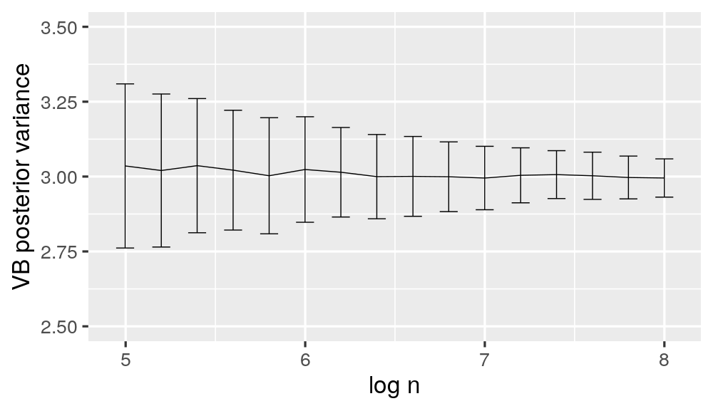
Refer to caption
(a) Variational variance of μ1\mu_{1} (with error bars).
Refer to caption
(b) Ratio of variances
Figure 3: Characterizations of the limiting variances in the mean-field approximation.

5.2 Bayesian Linear Regression

In this example we consider the Bayesian linear regression of the following form:

Yn=X​β+ε,ε∼N⁡(0,σ2​In).Y^{n}=X\beta+\varepsilon,\quad\varepsilon\sim N(0,\sigma^{2}I_{n}).

where YnY^{n} is the response vector in ℝn\mathbb{R}^{n}, and X=(X1,…,Xp)X=(X_{1},\ldots,X_{p}) is the design matrix of dimension n×pn\times p. We target at making inference on β=(β1,…,βp)∈ℝp\beta=(\beta_{1},\ldots,\beta_{p})\in\mathbb{R}^{p}, the regression coefficient vector. To facilitate variable selection, we impose independent point mass mixture priors for {βj}j=1p\{\beta_{j}\}_{j=1}^{p} by introducing pp latent binary variables {γj}j=1p\{\gamma_{j}\}_{j=1}^{p}, where γj\gamma_{j} indicates whether XjX_{j} is included in the model (or βj=0\beta_{j}=0 or not), that is,

βj|(γj=0,σ2)∼δ0andβj|(γj=1,σ2)∼N⁡(0,v1​σ2),\displaystyle\beta_{j}\,|\,(\gamma_{j}=0,\sigma^{2})\sim\delta_{0}\quad\mbox{and}\quad\beta_{j}|(\gamma_{j}=1,\sigma^{2})\sim N(0,v_{1}\sigma^{2}),

where δa\delta_{a} denotes the point mass measure at point aa. The prior for γj\gamma_{j}’s is specified as i.i.d. Bernoulli(ξ)(\xi), where ξ\xi follows the Beta prior distribution as Beta(a0,b0)(a_{0},b_{0}), and the prior for the noise variance σ2\sigma^{2} is the inverse Gamma distribution as IG(ν/2,ν​λ/2)(\nu/2,\nu\lambda/2). In our simulation, we take v1=2v_{1}=2, a0=1a_{0}=1, b0=1b_{0}=1, ν=0.002\nu=0.002 and λ=1\lambda=1 for the hyperparameters. In this example, there is no latent variable and the parameter is θ=({(γj,βj)}j=1p,σ2)\theta=(\{(\gamma_{j},\beta_{j})\}_{j=1}^{p},\sigma^{2}).

We apply the following block mean-field approximation [9] for approximating the joint posterior distribution p⁡({(γj,βj)}j=1p,σ2|Yn)p(\{(\gamma_{j},\beta_{j})\}_{j=1}^{p},\sigma^{2}\,|\,Y^{n}) using the blockwise-factorized family qθ=⨂j=1pqγj,βj⊗qσ2q_{\theta}=\bigotimes_{j=1}^{p}q_{\gamma_{j},\beta_{j}}\otimes q_{\sigma^{2}}. It again turns out that the point mass mixture priors on β\beta and inverse gamma prior on σ\sigma is the “conjugate” prior in the sense that in the KL minimizer q^θ=⨂j=1pq^γj,βj⊗q^σ2\widehat{q}_{\theta}=\bigotimes_{j=1}^{p}\widehat{q}_{\gamma_{j},\beta_{j}}\otimes\widehat{q}_{\sigma^{2}}, each q^γj,βj\widehat{q}_{\gamma_{j},\beta_{j}} is a point mass mixture and q^σ2\widehat{q}_{\sigma^{2}} is an inverse Gamma. Therefore, we can parametrize them by

Qγj,βj=(1−ϕj)​δ0​(γj)⊗δ0​(βj)+ϕj​δ1​(γj)⊗N⁡(μj,σj2),andQσ2=IG​(c,d),\displaystyle Q_{\gamma_{j},\beta_{j}}=(1-\phi_{j})\delta_{0}(\gamma_{j})\otimes\delta_{0}(\beta_{j})+\phi_{j}\delta_{1}(\gamma_{j})\otimes N(\mu_{j},\sigma_{j}^{2}),\ \ \mbox{and}\ \ Q_{\sigma^{2}}=\mbox{IG}(c,d), (22)

for j=1,…,pj=1,\ldots,p. Therefore, finding Q^θ\widehat{Q}_{\theta} amounts to optimizing the objective function (6) over these parameters {ϕj,μj,σj2)}j=1p\{\phi_{j},\mu_{j},\sigma_{j}^{2})\}_{j=1}^{p} and {c,d}\{c,d\} via the coordinate descent algorithm. Implementation details of the algorithm is provided in Appendix A.2, where we have adopted a slightly different but more efficient algorithm [18].

We generate the data in our simulation as follows. The number of observations is n=1,000n=1,000 and number of covariates p=10p=10, with ground truth parameter β∗=(2,3,2,4,1,2,1,0,0,2)T\beta^{\ast}=(2,3,2,4,1,2,1,0,0,2)^{T}. We generate XX conforming to an AR(1) process associated with a unit variance white noise process as below: for each i=1,…,ni=1,\ldots,n,

Xi​j=ρXi⁡(j−1)+εj,εj∼N(0,1)for j=2,…,p, andXi​1∼N(0,(1−ρ2)−1),X_{ij}=\rho X_{i(j-1)}+\varepsilon_{j},\ \ \varepsilon_{j}\sim N(0,1)\ \ \mbox{for $j=2,\ldots,p$, \ \ and}\ \ X_{i1}\sim N(0,(1-\rho^{2})^{-1}),

where ρ∈[0,1)\rho\in[0,1) is the auto-correlation, and each Xi​jX_{ij} has the same marginal distribution as N⁡(0,(1−ρ2)−1)N(0,(1-\rho^{2})^{-1}). In the simulation, we consider different settings of the auto-correlation as ρ=0,0.05,…,0.95\rho=0,0.05,\ldots,0.95. We draw B=1000B=1000 samples from the Gibbs sampler and the VWLB sampler (Algorithm 1). When evaluating four credible intervals, we compute the coverage probability based on 1,0001,000 replicates for each setting. Figure 4 reports the trends of coverage probabilities for two coefficients β1\beta_{1} and β4\beta_{4} using the four aforementioned types of credible intervals.

Refer to caption
(a) β1\beta_{1}
Refer to caption
(b) β4\beta_{4}
Figure 4: Coverage probabilities based on four types of credible intervals versus design correlation ρ\rho.

As we can expect, the coverage probabilities of the credible intervals based on the mean-field approximation Q^θ\widehat{Q}_{\theta} rapidly fall below the nominal level 95%95\% when the auto-correlation is large, as Q^θ\widehat{Q}_{\theta} completely ignores the (high) correlations among {βj}j=1p\{\beta_{j}\}_{j=1}^{p} in the joint posterior distribution Πn\Pi_{n}. In comparison, the rest three methods exhibit similar patterns and nearly attain the nominal level (horizontal dotted line) across all ρ\rho values. We also report the lengths of the intervals reflecting the estimated uncertainty magnitudes in Table 2.

β1\beta_{1} β4\beta_{4} β1\beta_{1} β4\beta_{4} β1\beta_{1} β4\beta_{4}
Gibbs Sampler 0.1245​(0.0066)0.1245(0.0066) 0.1243​(0.0064)0.1243(0.0064) 0.1243​(0.0064)0.1243(0.0064) 0.1388​(0.0071)0.1388(0.0071) 0.1222​(0.0099)0.1222(0.0099) 0.1675​(0.0174)0.1675(0.0174)
VB Posterior 0.1241​(0.0028)0.1241(0.0028) 0.1241​(0.0029)0.1241(0.0029) 0.1074​(0.0025)0.1074(0.0025) 0.1075​(0.0025)0.1075(0.0025) 0.0387​(0.0010)0.0387(0.0010) 0.0388​(0.0010)0.0388(0.0010)
VWLB Sampler 0.1223​(0.0070)0.1223(0.0070) 0.1226​(0.0070)0.1226(0.0070) 0.1223​(0.0071)0.1223(0.0071) 0.1368​(0.0077)0.1368(0.0077) 0.1218​(0.0071)0.1218(0.0071) 0.1680​(0.0097)0.1680(0.0097)
Table 2: Credible interval lengths for β1\beta_{1} and β4\beta_{4} under n=1,000n=1,000 and ρ∈{0,0.5,0.95}\rho\in\{0,0.5,0.95\}.

As we can infer from this table, the degree of uncertainty underestimation in the mean-field approximation Q^θ\widehat{Q}_{\theta} increases as the correlation among {βj}j=1p\{\beta_{j}\}_{j=1}^{p} in their joint posterior increases, as the posterior covariance matrix of the regression coefficient vector β\beta is approximately proportional to the auto-covariance matrix of the AR(1) process with auto-correlation ρ\rho. For example, when ρ=0\rho=0, there is no visible uncertainty underestimation, while when ρ=0.95\rho=0.95, the variational standard deviation of β4\beta_{4} reduces to roughly one quarter of the true (marginal) posterior standard deviation. In comparison, the lengths from Gibbs sampler and our VWLB sampler are always close.

6 Proofs of the main results

In this section, we provide a selective proofs of the main results in the paper, and leave the rest and some technique results to the supplement. To simplify the presentation, we use letter CC to denote a generic constant whose value may change from one line to another throughout the proof.

6.1 Proof of Lemma 2

Before showing that the variational approximation Q^θ\widehat{Q}_{\theta} has the desired sub-Gaussian type tail bound, we first show that the marginal posterior distribution Πn\Pi_{n} of θ\theta has a similar type bound. In fact, Assumption A2 implies Eθ∗​log⁡p⁡(X|θ∗)p⁡(X|θ)≤C​‖θ−θ∗‖2E_{\theta^{\ast}}\log\frac{p(X\,|\,\theta^{\ast})}{p(X\,|\,\theta)}\leq C\|\theta-\theta^{\ast}\|^{2} and Eθ∗​[log⁡p⁡(X|θ∗)p⁡(X|θ)]2≤C​‖θ−θ∗‖2E_{\theta^{\ast}}\big[\log\frac{p(X\,|\,\theta^{\ast})}{p(X\,|\,\theta)}\big]^{2}\leq C\|\theta-\theta^{\ast}\|^{2}. Therefore, we can apply Theorem 5.1 in [13] to obtain that for any M≥1M\geq 1, it holds with probability at least 1−C​M−21-CM^{-2} that the posterior Πn\Pi_{n} of θ\theta satisfies

Πn​(‖θ−θ∗‖≥C​ε)≤e−C​n​ε2,for all ε≥M​εn,\displaystyle\Pi_{n}\big(\|\theta-\theta^{\ast}\|\geq C\varepsilon\big)\leq e^{-Cn\varepsilon^{2}},\quad\mbox{for all $\varepsilon\geq M\varepsilon_{n}$}, (23)

where we slightly strengthen their result by providing the explicit posterior tail bound and by extending it from a single ε=M​εn\varepsilon=M\varepsilon_{n} to all ε≥M​εn\varepsilon\geq M\varepsilon_{n} simultaneously, due to the same argument as the proof of equation (6.10) in [41].

We will use the optimality of Q^=Q^Zn=Q^θ⊗Q^Sn\widehat{Q}=\widehat{Q}_{Z^{n}}=\widehat{Q}_{\theta}\otimes\widehat{Q}_{S^{n}} for optimization problem (6) to prove the desired result. Let Q|AQ|_{A} denote the restriction of a probability measure QQ onto a set A⊂Θ×𝒮nA\subset\Theta\times\mathcal{S}^{n}, that is, Q|A​(B)=Q⁡(A∩B)/Q⁡(A)Q|_{A}(B)=Q(A\cap B)/Q(A) for all B⊂Θ×𝒮nB\subset\Theta\times\mathcal{S}^{n}. For a fixed ε≥M​εn\varepsilon\geq M\varepsilon_{n} and each j=1,2,…,dj=1,2,\ldots,d, we construct a sequence 𝒬={Qλ†:λ∈[0,1]}\mathcal{Q}=\{Q^{\dagger}_{\lambda}:\,\lambda\in[0,1]\} of distributions as

Qλ†=(1−λ)​Q^|An,jc+λ​Q^|An,j,for all λ∈[0,1],\displaystyle Q^{\dagger}_{\lambda}=(1-\lambda)\,\widehat{Q}|_{A_{n,j}^{c}}+\lambda\,\widehat{Q}|_{A_{n,j}},\quad\mbox{for all $\lambda\in[0,1]$,}

where An,j={θ:|θj−θj∗|≥D​ε}×𝒮nA_{n,j}=\{\theta:\,|\theta_{j}-\theta^{\ast}_{j}|\geq D\varepsilon\}\times\mathcal{S}^{n} for some sufficiently large constant D≥CD\geq C. It is easy to verify that Qλ†Q^{\dagger}_{\lambda} is a valid distribution belonging to the mean-field family Γ\Gamma for any λ∈[0,1]\lambda\in[0,1]. Let λ^=Q^​(An,j)\widehat{\lambda}=\widehat{Q}(A_{n,j}), so that Q^=Qλ^†\widehat{Q}=Q^{\dagger}_{\widehat{\lambda}}. Due to the optimality of Q^\widehat{Q} for minimizing D(Q||P(⋅|Xn))D\big(Q\,||\,P(\cdot\,|\,X^{n})\big) when restricting to the smaller family 𝒬\mathcal{Q}, we obtain λ^=argminλ∈[0,1]D(Qλ†||P(⋅|Xn))\widehat{\lambda}=\mathop{\rm argmin~}_{\lambda\in[0,1]}D\big(Q^{\dagger}_{\lambda}\,||\,P(\cdot\,|\,X^{n})\big), where we can express

D(Qλ†∥P(⋅|Xn))=∫Θ×𝒮nlog⁡(Qλ†​(dZn)P⁡(dZn|Xn))[(1−λ)Q^|An,jc(dZn)+λQ^|An,j(dZn)]\displaystyle D\big(Q_{\lambda}^{\dagger}\,\|\,P(\cdot\,|\,X^{n})\big)=\int_{\Theta\times\mathcal{S}^{n}}\log(\frac{Q^\dagger_{\lambda}(\dd Z^n)}{ P(\dd Z^n\,|\,X^n)})\,\big[(1-\lambda)\,\widehat{Q}|_{A_{n,j}^{c}}(\differential Z^{n})+\lambda\,\widehat{Q}|_{A_{n,j}}(\differential Z^{n})\big]
=(1−λ)​∫An,jclog⁡((1−λ)​Q^|An,jc​(dZn)P⁡(dZn|Xn))​Q^|An,jc​(dZn)+λ​∫An,jlog⁡(λ​Q^|An,j​(dZn)P⁡(dZn|Xn))​Q^|An,j​(dZn),\displaystyle\quad=(1-\lambda)\int_{A_{n,j}^{c}}\log(\frac{(1 - \lambda)\,\wht{Q}|_{A_{n,j}^c}(\dd Z^n)}{P(\dd Z^n\,|\,X^n)})\,\widehat{Q}|_{A_{n,j}^{c}}(\differential Z^{n})+\lambda\int_{A_{n,j}}\log(\frac{\lambda\,\wht{Q}|_{A_{n,j}}(\dd Z^n)}{P(\dd Z^n\,|\,X^n)})\,\widehat{Q}|_{A_{n,j}}(\differential Z^{n}),

where the second equality is due to mutual orthogonality of Q^|An,j\widehat{Q}|_{A_{n,j}} and Q^|An,jc\widehat{Q}|_{A_{n,j}^{c}}. Due to a similar decomposition P⁡(dZn|Xn)=P|An,j​(dZn|Xn)​P​(An,j|Xn)+P|An,jc​(dZn|Xn)​P​(An,jc|Xn)P(\differential Z^{n}\,|\,X^{n})=P|_{A_{n,j}}(\differential Z^{n}\,|\,X^{n})\,P(A_{n,j}\,|\,X^{n})+P|_{A_{n,j}^{c}}(\differential Z^{n}\,|\,X^{n})\,P(A_{n,j}^{c}\,|\,X^{n}) for P⁡(dZ|Xn)P(\differential Z\,|\,X^{n}), the preceding display can be further decomposed into

(1−λ)​∫An,jclog⁡(Q^|An,jc​(dZn)P|An,jc​(dZn|Xn))​Q^|An,jc​(dZn)+λ​∫An,jlog⁡(Q^|An,j​(dZn)PAn,j​(dZn|Xn))​Q^|An,j​(dZn)\displaystyle(1-\lambda)\int_{A_{n,j}^{c}}\log(\frac{\wht{Q}|_{A_{n,j}^c}(\dd Z^n)}{P|_{A_{n,j}^c}(\dd Z^n\,|\,X^n)})\,\widehat{Q}|_{A_{n,j}^{c}}(\differential Z^{n})+\lambda\int_{A_{n,j}}\log(\frac{\wht{Q}|_{A_{n,j}}(\dd Z^n)}{P_{A_{n,j}}(\dd Z^n\,|\,X^n)})\,\widehat{Q}|_{A_{n,j}}(\differential Z^{n})
+(1−λ)​log⁡(1−λP⁡(An,jc|Xn))+λ​log⁡(λP⁡(An,j|Xn))\displaystyle\qquad\qquad\qquad\qquad\qquad\qquad\qquad+(1-\lambda)\log(\frac{1-\lambda}{P(A_{n,j}^c\,|\,X^n)})+\lambda\log(\frac{\lambda}{P(A_{n,j}\,|\,X^n)})
=\displaystyle= (1−λ)dn​2+λdn​1+D(Ber(λ)∥Ber(βn)),\displaystyle(1-\lambda)\,d_{n2}+\lambda\,d_{n1}+D\big(\text{Ber}(\lambda)\,\|\,\text{Ber}(\beta_{n})\big), (24)

where βn=P⁡(An,j|Xn)=Πn​(|θj−θj∗|≥D​ε)\beta_{n}=P(A_{n,j}\,|\,X^{n})=\Pi_{n}(|\theta_{j}-\theta^{\ast}_{j}|\geq D\varepsilon), Ber​(λ)\text{Ber}(\lambda) denotes a Bernoulli distribution with success probability λ\lambda, and two constants (dn​1,dn​2)(d_{n1},d_{n2}) independent of λ\lambda are

dn​1=D(Q^|An,j∥P|An,j(⋅|Xn))anddn​2=D(Q^|An,jc∥P|An,jc(⋅|Xn)).\displaystyle d_{n1}=D\big(\widehat{Q}|_{A_{n,j}}\,\|P|_{A_{n,j}}(\cdot\,|\,X^{n})\big)\quad\mbox{and}\quad d_{n2}=D\big(\widehat{Q}|_{A_{n,j}^{c}}\,\|P|_{A_{n,j}^{c}}(\cdot\,|\,X^{n})\big).

Since λ^\widehat{\lambda} minimizes D(Qλ†∥P(⋅|Xn))D\big(Q_{\lambda}^{\dagger}\,\|\,P(\cdot\,|\,X^{n})\big), by setting the derivative of (24) as a function of λ\lambda to be zero, we obtain

λ^=\displaystyle\widehat{\lambda}= βn​exp⁡(−dn​1)βn​exp⁡(−dn​1)+(1−βn)​exp⁡(−dn​2)≤βn​exp⁡(−dn​1)(1−βn)​exp⁡(−dn​2)≤βn1−βn​exp⁡(dn​2),\displaystyle\,\frac{\beta_{n}\,\exp(-d_{n1})}{\beta_{n}\,\exp(-d_{n1})+(1-\beta_{n})\,\exp(-d_{n2})}\leq\frac{\beta_{n}\,\exp(-d_{n1})}{(1-\beta_{n})\,\exp(-d_{n2})}\leq\frac{\beta_{n}}{1-\beta_{n}}\exp(d_{n2}),

where we have used the fact that dn​1≥0d_{n1}\geq 0 in the last step. On the other hand, from the fact that (24) is equal to D(Qλ†∥P(⋅|Xn))D\big(Q_{\lambda}^{\dagger}\,\|\,P(\cdot\,|\,X^{n})\big) at λ=λ^\lambda=\widehat{\lambda} and the non-negativeness of the three terms therein, we obtain D(Q^||P(⋅|Xn))≥(1−λ^)dn​2+D(Ber(λ^)∥Ber(βn))D\big(\widehat{Q}\,||\,P(\cdot\,|\,X^{n})\big)\geq(1-\widehat{\lambda})\,d_{n2}+D\big(\text{Ber}(\widehat{\lambda})\,\|\,\text{Ber}(\beta_{n})\big). Combining this with the preceding display, we can reach

λ^≤2βnexp⁡(D(Q^∥P(⋅|Xn))1−λ^)andD(Ber(λ^)∥Ber(βn))≤D(Q^∥P(⋅|Xn)),\displaystyle\widehat{\lambda}\leq 2\beta_{n}\exp(\frac{D\big(\wht{Q}\, \| \,P(\cdot\,|\,X^n))}{1 - \wht{\lambda}})\quad\mbox{and}\quad D\big(\text{Ber}(\widehat{\lambda})\,\|\,\text{Ber}(\beta_{n})\big)\leq D\big(\widehat{Q}\,\|\,P(\cdot\,|\,X^{n})), (25)

where we have used inequality (23) so that βn≤Πn​(‖θ−θ∗‖≥D​ε)≤e−C​D2​n​ε2≤n−C​D2≤1/2\beta_{n}\leq\Pi_{n}(\|\theta-\theta^{\ast}\|\geq D\varepsilon)\leq e^{-CD^{2}n\varepsilon^{2}}\leq n^{-CD^{2}}\leq 1/2 for a sufficiently large DD.

Now we invoke the following lemma for bounding D(Q^∥Πn)D\big(\widehat{Q}\,\|\,\Pi_{n}) from above. Its proof is deferred to Appendix B.9 in the supplement.

Lemma 4.

Under Assumptions A1, A2 and A3, it holds with probability at least 1−C​M−21-CM^{-2} that

D(Q^∥P(⋅|Xn))≤CnM2εn2.\displaystyle D\big(\widehat{Q}\,\|\,P(\cdot\,|\,X^{n}))\leq CnM^{2}\varepsilon_{n}^{2}.

Using this lemma, the second display in inequality (25), the bound in inequality (23) on βn\beta_{n}, and the fact that λ​log⁡λ+(1−λ)​log⁡(1−λ)≥−log⁡2\lambda\log\lambda+(1-\lambda)\log(1-\lambda)\geq-\log 2 for any λ∈[0,1]\lambda\in[0,1], we can obtain that λ^≤C/D2≤1/2\widehat{\lambda}\leq C/D^{2}\leq 1/2 by choosing a sufficiently large DD. Then a combination of the same Lemma 4, the inequality (23) on βn\beta_{n}, and the first display in inequality (25) on λ^\widehat{\lambda} implies

Q^θ​(|θj−θj∗|≥D​ε)=λ^≤2​exp⁡(−C​D2​n​ε2+2​C​n​M2​εn2)≤exp(−CD2nε2/2),\displaystyle\widehat{Q}_{\theta}(|\theta_{j}-\theta^{\ast}_{j}|\geq D\varepsilon)=\widehat{\lambda}\leq 2\exp(-CD^2 n\,\varepsilon^2 + 2CnM^2\varepsilon_n^2)\leq\exp(-CD^2n\varepsilon^2/2),

for a sufficiently large constant DD, which yields the claimed result on the tail probability of Q^θ\widehat{Q}_{\theta} via a union bound over j=1,…,dj=1,\ldots,d (since d−1/2∥θ−θ∗∥≤maxj|θj−θj∗|d^{-1/2}\|\theta-\theta^{\ast}\|\leq\max_{j}|\theta_{j}-\theta_{j}^{\ast}|).

6.2 Proof of Theorem 1

We focus on illustrating the key proof idea of Theorem 1 in this subsection, and leave the proofs of technical lemmas to the appendix. In addition, the proof of Theorem 4 (weighted version of Theorem 1) will follow the same strategy, and details are also deferred to Appendix B.6.

One main difficulty of the proof lies in the fact that the KL divergence does not satisfy the triangle inequality (unless the approximate family is convex, which is not true in the mean-field case), when specialized to our problem, taking the form as

D(Q^θ||QV​B∗)≤D(Q^θ||N(θ^MLE,[nIc(θ∗)]−1))−D(QV​B∗||N(θ^MLE,[nIc(θ∗)]−1)),\displaystyle D(\widehat{Q}_{\theta}\,||\,Q^{\ast}_{VB})\leq D\big(\widehat{Q}_{\theta}\,||\,N(\widehat{\theta}_{\mbox{\tiny MLE}},\,[nI_{c}(\theta^{\ast})]^{-1})\big)-D\big(Q^{\ast}_{VB}\,||\,N(\widehat{\theta}_{\mbox{\tiny MLE}},\,[nI_{c}(\theta^{\ast})]^{-1})\big),

where recall that QV​B∗Q^{\ast}_{VB} shares the same center θ^MLE\widehat{\theta}_{\mbox{\tiny MLE}} as N⁡(θ^MLE,[n​Ic​(θ∗)]−1)N(\widehat{\theta}_{\mbox{\tiny MLE}},\,[nI_{c}(\theta^{\ast})]^{-1}), but the precision matrix (inverse of covariance matrix) of the former is the diagonal part of the latter. This triangle inequality, if true, would imply the desired bound on D(Q^θ||QV​B∗)D(\widehat{Q}_{\theta}\,||\,Q^{\ast}_{VB}). In fact, according to Lemma 5 below, QV​B∗Q^{\ast}_{VB} minimizes D(Qθ||N(θ^MLE,[nIc(θ∗)]−1)D\big(Q_{\theta}\,||\,N(\widehat{\theta}_{\mbox{\tiny MLE}},\,[nI_{c}(\theta^{\ast})]^{-1}\big) over all QθQ_{\theta} within the mean-field family (QθQ_{\theta} factorizes into ⨂j=1dQθj\bigotimes_{j=1}^{d}Q_{\theta_{j}}). Moreover, the variational optimum Q^θ\widehat{Q}_{\theta} also approximately minimizes this divergence since according to Lemma 6, the KL divergence D(Qθ||N(θ^MLE,[nIc(θ∗)]−1))D\big(Q_{\theta}\,||\,N(\widehat{\theta}_{\mbox{\tiny MLE}},\,[nI_{c}(\theta^{\ast})]^{-1})\big) is, for all QθQ_{\theta} with a similar sub-Gaussian tail as in Lemma 2, close to the “profile divergence” defined in Lemma 1, for which Q^θ\widehat{Q}_{\theta} is the minimizer since by definition (Q^θ,Q^Sn)(\widehat{Q}_{\theta},\widehat{Q}_{S^{n}}) jointly minimizes the variational objective function (7). In other words, the preceding triangle inequality reveals the local strongly convexity structure of the profile variational objective function (after profiling out QSnQ_{S^{n}}) around the populational level minimizer QV​B∗Q^{\ast}_{VB}. Unfortunately, such a triangle inequality for KL divergence is not true in general. Therefore, our first step of the proof is to establish a similar “triangle inequality” restricted on the mean-field family with respect to the KL-divergence around the populational level minimizer QV​B∗Q^{\ast}_{VB}. After that, we will formalize the above intuition that Q^θ\widehat{Q}_{\theta} effectively minimizes D(Qθ||N(θ^MLE,[nIc(θ∗)]−1))D\big(Q_{\theta}\,||\,N(\widehat{\theta}_{\mbox{\tiny MLE}},\,[nI_{c}(\theta^{\ast})]^{-1})\big).

Step one: In this step, we build a “triangle inequality” for the KL-divergence restricting to the mean-field family. We will repeatedly use the following decomposition of the KL-divergence D(Q||P)D(Q\,||\,P) when the first probability measure QQ belongs to the mean-field family and the second probability measure PP is a normal distribution. Here we use the notation μQθ\mu_{Q_{\theta}} to denote the expectation of any probability measure QQ over a space Θ\Theta, and for any vector u∈Θu\in\Theta, use QuQ_{u} to denote the translation of QQ whose expectation is uu, that is, Q⁡(A+μQθ)=Q(u)​(A+u)Q(A+\mu_{Q_{\theta}})=Q_{(u)}(A+u) for any measurable set A⊂ΘA\subset\Theta. Let λmin​(Γ)\lambda_{\min}(\Gamma) denote the smallest eigenvalue of a positive definite matrix Γ\Gamma.

Lemma 5.

Let QQ be a probability measure on ℝd\mathbb{R}^{d} that factorizes as Q=⨂j=1dQjQ=\bigotimes_{j=1}^{d}Q_{j}, μ∈ℝd\mu\in\mathbb{R}^{d} be a dd-dim vector and Γ∈ℝd×d\Gamma\in\mathbb{R}^{d\times d} a dd-by-dd positive definite matrix. Let 𝑂𝑃𝐸𝑁Q∗=N⁡(μ,(diag​(Γ))−1))=⨂j=1dQj∗Q^{\ast}=N(\mu,(\text{diag}(\Gamma))^{-1}))=\bigotimes_{j=1}^{d}Q^{\ast}_{j}, where Qj∗Q^{\ast}_{j} is the univariate normal distribution N⁡(μj,Γj​j−1)N(\mu_{j},\Gamma_{jj}^{-1}) for j=1,…,dj=1,\ldots,d. Then we have the decomposition

D(Q||N(μ,Γ−1))−D(Q∗||N(μ,Γ−1))=∑j=1dD(Q(μj),j||Qj∗)+12(μQθ−μ)TΓ(μQθ−μ),\displaystyle D\big(Q\,||\,N(\mu,\,\Gamma^{-1})\big)-D\big(Q^{\ast}\,||\,N(\mu,\,\Gamma^{-1})\big)=\sum_{j=1}^{d}D\big(Q_{(\mu_{j}),j}\,||\,Q^{\ast}_{j}\big)+\frac{1}{2}(\mu_{Q_{\theta}}-\mu)^{T}\Gamma\,(\mu_{Q_{\theta}}-\mu),

where μQθ∈ℝd\mu_{Q_{\theta}}\in\mathbb{R}^{d} denotes the expectation of QQ. Furthermore, we have

D(Q∥Q∗)≤maxj⁡Γj​jλmin​(Γ)[D(Q∥N(μ,Γ−1))−D(Q∗∥N(μ,Γ−1))].\displaystyle D(Q\,\|\,Q^{\ast})\leq\frac{\max_{j}\Gamma_{jj}}{\lambda_{\min}(\Gamma)}\,\bigl[D(Q\,\|\,N(\mu,\Gamma^{-1}))-D(Q^{\ast}\,\|\,N(\mu,\Gamma^{-1}))\bigr].

Our proof based on direct calculation is provided in Appendix B.10. As a direct consequence, the first identity in the lemma implies that Q∗Q^{\ast} minimizes D(Q||N(μ,Γ−1))D\big(Q\,||\,N(\mu,\,\Gamma^{-1})\big) over all QQ within the mean-field family. When the covariance matrix Γ\Gamma is a multiple of the identity matrix, the second inequality in the lemma has leading factor 11 and becomes the triangle inequality for the KL divergence at Q∗Q^{\ast}. We will apply this result with Q∗Q^{\ast} as QV​B∗Q^{\ast}_{VB} and N⁡(μ,Γ−1)=N⁡(θ^MLE,[n​Ic​(θ∗)]−1)N(\mu,\Gamma^{-1})=N\big(\widehat{\theta}_{\mbox{\tiny MLE}},[nI_{c}(\theta^{\ast})]^{-1}\big) below in the proof.

Step two: In this step, we study the profile divergence defined in Lemma 1. Specifically, let Fn(Qθ)=minQSn=⨂i=1nQSiD(Qθ⊗QSn∥P(⋅|Xn))F_{n}(Q_{\theta})=\min_{Q_{S^{n}}=\bigotimes_{i=1}^{n}Q_{S_{i}}}D\big(Q_{\theta}\otimes Q_{S^{n}}\,\|\,P(\cdot\,|\,X^{n})\big) be the profile divergence. The following lemma provides an approximation formula for Fn​(Qθ)F_{n}(Q_{\theta}) for all QθQ_{\theta} with a suitable tail decay property. Here, for any probability measure QQ, we use ΣQ\Sigma_{Q} to denote the dd-by-dd covariance matrix of QQ. In particular, ΣQ\Sigma_{Q} becomes diagonal when QQ belongs to the mean-field family.

Lemma 6.

Suppose Assumption A3 holds. Then for any M≥1M\geq 1, it holds with probability at least 1−C​M−21-CM^{-2} that for any probability measure Q=⨂j=1dQjQ=\bigotimes_{j=1}^{d}Q_{j} satisfying the same sub-Gaussian tail decay as in Lemma 2, we have

|Fn(Qθ)−D(Qθ||Πn)−n2tr(ΣQθIs(θ∗))|≤C​M3​(log⁡n)3/2n,\displaystyle\Big|F_{n}(Q_{\theta})-D\big(Q_{\theta}\,||\,\Pi_{n}\big)-\frac{n}{2}\,\text{tr}\big(\Sigma_{Q_{\theta}}\,I_{s}(\theta^{\ast})\big)\Big|\leq\frac{CM^{3}(\log n)^{3/2}}{\sqrt{n}},

where Is​(θ∗)I_{s}(\theta^{\ast}) is defined in Assumption A3.

The proof is deferred to Appendix B.11 based on Taylor expansions. When there is no latent variable, Fn​(Qθ)F_{n}(Q_{\theta}) is exactly D(Qθ||Πn)D\big(Q_{\theta}\,||\,\Pi_{n}\big). This means that the third extra term n2​tr​(ΣQθ​Is​(θ∗))\frac{n}{2}\,\text{tr}\big(\Sigma_{Q_{\theta}}\,I_{s}(\theta^{\ast})\big) is due to the mean-field approximation between the parameter θ\theta and latent variables SnS^{n}. This third term is not negligible since it will contribute to the precision matrix n​IV​BnI_{VB} of the normal approximation QV​B∗Q^{\ast}_{VB} to Q^θ\widehat{Q}_{\theta}, as we will show in the following steps.

Step three: The marginal posterior distribution Πn\Pi_{n} of θ\theta in the approximation of Fn​(Qθ)F_{n}(Q_{\theta}) in Lemma 6 is not convenient for our analysis. However, from the classical Bernstein von-Mises theorem, Πn\Pi_{n} should be well approximated by a normal distribution N⁡(θ^MLE,[n​I​(θ∗)]−1)N\big(\widehat{\theta}_{\mbox{\tiny MLE}},\,[nI(\theta^{\ast})]^{-1}\big). The following lemma shows that for any QθQ_{\theta} with a suitable tail decay property, D(Qθ||N(θ^MLE,[nI(θ∗)]−1))D\big(Q_{\theta}\,||\,N\big(\widehat{\theta}_{\mbox{\tiny MLE}},\,[nI(\theta^{\ast})]^{-1}\big)\big) provides a good approximation to D(Qθ||Πn)D\big(Q_{\theta}\,||\,\Pi_{n}\big). Note that this lemma only assumes a sub-Gaussian type tail but not the mean-field structure (therefore it implies a KL divergence version of the BvM theorem). Then we may apply the first identity in Lemma 5 to analyze this KL divergence term.

Lemma 7.

Suppose Assumptions A1 and A2 hold. Then for any M≥1M\geq 1, it holds with probability at least 1−C​M−21-CM^{-2} that for any probability measure QθQ_{\theta} satisfying the same sub-Gaussian tail decay as in Lemma 2, we have

|D(Qθ||Πn)−D(Qθ||N(θ^MLE,[nI(θ∗)]−1))|≤C​M3​(log⁡n)d+3n,\displaystyle\Big|D\big(Q_{\theta}\,||\,\Pi_{n}\big)-D\big(Q_{\theta}\,||\,N\big(\widehat{\theta}_{\mbox{\tiny MLE}},\,[nI(\theta^{\ast})]^{-1}\big)\big)\Big|\leq\frac{CM^{3}(\log n)^{d+3}}{\sqrt{n}},

where I⁡(θ∗)I(\theta^{\ast}) is the information matrix defined in Assumption A2.

The proof of this lemma is provided in Appendix B.12. In particular, we will apply this lemma with QθQ_{\theta} as Q^θ\widehat{Q}_{\theta} and QV​B∗Q^{\ast}_{VB} that both satisfy the sub-Gaussian tail decay property in Lemma 2.

Step four: Let αn=C​M3​(log⁡n)d+3n\alpha_{n}=\frac{CM^{3}(\log n)^{d+3}}{\sqrt{n}} denote the error upper bound in Lemmas 6 and 7. In this step, we will formalize the intuition that Q^θ\widehat{Q}_{\theta} effectively minimizes D(Qθ||N(θ^MLE,[nIc(θ∗)]−1))D\big(Q_{\theta}\,||\,N(\widehat{\theta}_{\mbox{\tiny MLE}},\,[nI_{c}(\theta^{\ast})]^{-1})\big). For any Q=⨂j=1dQjQ=\bigotimes_{j=1}^{d}Q_{j} satisfying the same sub-Gaussian tail decay as in Lemma 2, we have by Lemmas 6 and 7 that

|Fn(Qθ)−D(Qθ||N(θ^MLE,[nI(θ∗)]−1))−n2tr(ΣQθIs(θ∗))|\displaystyle\Big|\,F_{n}(Q_{\theta})-D\big(Q_{\theta}\,||\,N\big(\widehat{\theta}_{\mbox{\tiny MLE}},\,[nI(\theta^{\ast})]^{-1}\big)\big)-\frac{n}{2}\,\text{tr}\big(\Sigma_{Q_{\theta}}\,I_{s}(\theta^{\ast})\big)\Big| ≤2​αn.\displaystyle\leq 2\alpha_{n}. (26)

This inequality indicates that Q^θ\widehat{Q}_{\theta} is effectively minimizing the (negative) sum of the second and third terms in it, since Q^θ\widehat{Q}_{\theta} minimizes Fn​(Qθ)F_{n}(Q_{\theta}). Next we will relate this approximate objective function with D(Qθ||N(θ^MLE,[nIc(θ∗)]−1))D\big(Q_{\theta}\,||\,N(\widehat{\theta}_{\mbox{\tiny MLE}},\,[nI_{c}(\theta^{\ast})]^{-1})\big).

Using equation (44) twice in the proof of Lemma 5 in Appendix B.10 with (μ,Γ)=(θ^MLE,n​Ic​(θ∗))(\mu,\Gamma)=(\widehat{\theta}_{\mbox{\tiny MLE}},nI_{c}(\theta^{\ast})) and with (μ,Γ)=(θ^MLE,n​I​(θ∗))(\mu,\Gamma)=(\widehat{\theta}_{\mbox{\tiny MLE}},nI(\theta^{\ast})), respectively, we obtain

D(Qθ||N(θ^MLE,[nIc(θ∗)]−1))=∑j=1d∫ℝqj(θj)logqj(θj)dθj+12log⁡((2​π)d​|n​Ic​(θ∗)|−1)\displaystyle D\big(Q_{\theta}\,||\,N\big(\widehat{\theta}_{\mbox{\tiny MLE}},\,[nI_{c}(\theta^{\ast})]^{-1}\big)\big)=\sum_{j=1}^{d}\int_{\mathbb{R}}q_{j}(\theta_{j})\log q_{j}(\theta_{j})\,\differential\theta_{j}+\frac{1}{2}\log\big((2\pi)^{d} |n I_c(\theta^\ast)|^{-1}\big)
+n2​tr​(ΣQθ​Ic​(θ∗))+n2​(μQθ−θ^MLE)T​Ic​(θ∗)​(μQθ−θ^MLE),\displaystyle\qquad\qquad\qquad\qquad\qquad\qquad\qquad\qquad+\frac{n}{2}\,\text{tr}\big(\Sigma_{Q_{\theta}}\,I_{c}(\theta^{\ast})\big)+\frac{n}{2}(\mu_{Q_{\theta}}-\widehat{\theta}_{\mbox{\tiny MLE}})^{T}I_{c}(\theta^{\ast})\,(\mu_{Q_{\theta}}-\widehat{\theta}_{\mbox{\tiny MLE}}),
D(Qθ||N(θ^MLE,[nI(θ∗)]−1))=∑j=1d∫ℝqj(θj)logqj(θj)dθj+12log⁡((2​π)d​|n​I​(θ∗)|−1)\displaystyle D\big(Q_{\theta}\,||\,N\big(\widehat{\theta}_{\mbox{\tiny MLE}},\,[nI(\theta^{\ast})]^{-1}\big)\big)=\sum_{j=1}^{d}\int_{\mathbb{R}}q_{j}(\theta_{j})\log q_{j}(\theta_{j})\,\differential\theta_{j}+\frac{1}{2}\log\big((2\pi)^{d} |n I(\theta^\ast)|^{-1}\big)
+n2​tr​(ΣQθ​I​(θ∗))+n2​(μQθ−θ^MLE)T​I​(θ∗)​(μQθ−θ^MLE),\displaystyle\qquad\qquad\qquad\qquad\qquad\qquad\qquad\qquad+\frac{n}{2}\,\text{tr}\big(\Sigma_{Q_{\theta}}\,I(\theta^{\ast})\big)+\frac{n}{2}(\mu_{Q_{\theta}}-\widehat{\theta}_{\mbox{\tiny MLE}})^{T}I(\theta^{\ast})\,(\mu_{Q_{\theta}}-\widehat{\theta}_{\mbox{\tiny MLE}}),

where we have used the fact that ΣQθ\Sigma_{Q_{\theta}} is a diagonal matrix, so that we can express the sum as the trace. Taking the difference between two and using the fact that Ic​(θ∗)=I⁡(θ∗)+Is​(θ∗)I_{c}(\theta^{\ast})=I(\theta^{\ast})+I_{s}(\theta^{\ast}), we can further obtain by rearranging the terms that

D(Qθ||N(θ^MLE,[nI(θ∗)]−1))+n2tr(ΣQθIs(θ∗))\displaystyle D\big(Q_{\theta}\,||\,N\big(\widehat{\theta}_{\mbox{\tiny MLE}},\,[nI(\theta^{\ast})]^{-1}\big)\big)+\frac{n}{2}\,\text{tr}\big(\Sigma_{Q_{\theta}}\,I_{s}(\theta^{\ast})\big) (27)
=\displaystyle= D(Qθ||N(θ^MLE,[nIc(θ∗)]−1))−n2(μQθ−θ^MLE)TIs(θ∗)(μQθ−θ^MLE)+Rc,\displaystyle D\big(Q_{\theta}\,||\,N\big(\widehat{\theta}_{\mbox{\tiny MLE}},\,[nI_{c}(\theta^{\ast})]^{-1}\big)\big)-\frac{n}{2}(\mu_{Q_{\theta}}-\widehat{\theta}_{\mbox{\tiny MLE}})^{T}I_{s}(\theta^{\ast})\,(\mu_{Q_{\theta}}-\widehat{\theta}_{\mbox{\tiny MLE}})+R_{c},

where Rc=12​log⁡(|Ic​(θ∗)|⋅|I⁡(θ∗)|−1)R_{c}=\frac{1}{2}\log\big( |I_c(\theta^\ast)|\cdot|I(\theta^\ast)|^{-1}\big) is a constant independent of QθQ_{\theta}. A combination of this identity with inequality (26) indicates that up to a translation, Q^θ\widehat{Q}_{\theta} minimizes D(Qθ||N(θ^MLE,[nIc(θ∗)]−1))D\big(Q_{\theta}\,||\,N(\widehat{\theta}_{\mbox{\tiny MLE}},\,[nI_{c}(\theta^{\ast})]^{-1})\big). Moreover, the first identity in Lemma 5 indicates that the KL-divergence also contains a translation related term (second term) that strictly dominates −n2​(μQθ−θ^MLE)T​Is​(θ∗)​(μQθ−θ^MLE)-\frac{n}{2}(\mu_{Q_{\theta}}-\widehat{\theta}_{\mbox{\tiny MLE}})^{T}I_{s}(\theta^{\ast})\,(\mu_{Q_{\theta}}-\widehat{\theta}_{\mbox{\tiny MLE}}), so that the center can still be captured by minimizing Fn​(Qθ)F_{n}(Q_{\theta}), as we will show in the next step below.

Step five: This is the last step where we will use the optimality of Q^\widehat{Q} to prove the claimed bound. More specifically, by the optimaility of Q^θ\widehat{Q}_{\theta} and the feasibility of QV​B∗Q^{\ast}_{VB} for the optimization problem minQθ=⨂Qθj⁡Fn​(Qθ)\min_{Q_{\theta}=\bigotimes Q_{\theta_{j}}}F_{n}(Q_{\theta}), we obtain

Fn​(Q^)≤Fn​(QV​B∗).\displaystyle F_{n}(\widehat{Q})\leq F_{n}(Q^{\ast}_{VB}). (28)

Combining this inequality with (26) and (27) and using the fact that both Q^θ\widehat{Q}_{\theta} (by Lemma 2) and QV​B∗Q^{\ast}_{VB} satisfy the sub-Gaussian tail condition therein, we can reach

D(Q^θ||N(θ^MLE,[nIc(θ∗)]−1))−n2(μQ^θ−θ^MLE)TIs(θ∗)(μQ^θ−θ^MLE)\displaystyle D\big(\widehat{Q}_{\theta}\,||\,N\big(\widehat{\theta}_{\mbox{\tiny MLE}},\,[nI_{c}(\theta^{\ast})]^{-1}\big)\big)-\frac{n}{2}(\mu_{\widehat{Q}_{\theta}}-\widehat{\theta}_{\mbox{\tiny MLE}})^{T}I_{s}(\theta^{\ast})\,(\mu_{\widehat{Q}_{\theta}}-\widehat{\theta}_{\mbox{\tiny MLE}}) (29)
≤D(Q∗V​B||N(θ^MLE,[nIc(θ∗)]−1))+4αn,\displaystyle\leq D\big(Q^{\ast}_{VB}\,||\,N\big(\widehat{\theta}_{\mbox{\tiny MLE}},\,[nI_{c}(\theta^{\ast})]^{-1}\big)\big)+4\alpha_{n},

where we have used the fact that the mean of QV​B∗Q^{\ast}_{VB} is θ^MLE\widehat{\theta}_{\mbox{\tiny MLE}}. Now we combine the above with the first identity in Lemma 5 with (μ,Γ)=(θ^MLE,n​Ic​(θ∗))(\mu,\Gamma)=(\widehat{\theta}_{\mbox{\tiny MLE}},nI_{c}(\theta^{\ast})) so that Q∗=QV​B∗Q^{\ast}=Q^{\ast}_{VB} to obtain,

n2​(μQ^θ−θ^MLE)T​I​(θ∗)​(μQ^θ−θ^MLE)≤4​αn,\displaystyle\frac{n}{2}(\mu_{\widehat{Q}_{\theta}}-\widehat{\theta}_{\mbox{\tiny MLE}})^{T}I(\theta^{\ast})\,(\mu_{\widehat{Q}_{\theta}}-\widehat{\theta}_{\mbox{\tiny MLE}})\leq 4\alpha_{n}, (30)

where we have used the nonnegativeness of KL divergence. Since I⁡(θ∗)I(\theta^{\ast}) is positive definite by Assumption A2, we have from the above that for some constant C>0C>0,

n2​(μQ^θ−θ^MLE)T​Is​(θ∗)​(μQ^θ−θ^MLE)≤C​αn,\displaystyle\frac{n}{2}(\mu_{\widehat{Q}_{\theta}}-\widehat{\theta}_{\mbox{\tiny MLE}})^{T}I_{s}(\theta^{\ast})\,(\mu_{\widehat{Q}_{\theta}}-\widehat{\theta}_{\mbox{\tiny MLE}})\leq C\alpha_{n},

Finally, by combining the preceding display, inequality (29) and the second inequality in Lemma 5, we obtain

D(Q^θ||QV​B∗)\displaystyle D\big(\widehat{Q}_{\theta}\,||\,Q^{\ast}_{VB}\big) ≤C[D(Q^θ||N(θ^MLE,[nIc(θ∗)]−1))−D(QV​B∗||N(θ^MLE,[nIc(θ∗)]−1))]\displaystyle\leq C\,\Big[D\big(\widehat{Q}_{\theta}\,||\,N\big(\widehat{\theta}_{\mbox{\tiny MLE}},\,[nI_{c}(\theta^{\ast})]^{-1}\big)\big)-D\big(Q^{\ast}_{VB}\,||\,N\big(\widehat{\theta}_{\mbox{\tiny MLE}},\,[nI_{c}(\theta^{\ast})]^{-1}\big)\big)\Big]
≤C​αn+n2​(μQ^θ−θ^MLE)T​Is​(θ∗)​(μQ^θ−θ^MLE)≤C′​αn,\displaystyle\leq C\alpha_{n}+\frac{n}{2}(\mu_{\widehat{Q}_{\theta}}-\widehat{\theta}_{\mbox{\tiny MLE}})^{T}I_{s}(\theta^{\ast})\,(\mu_{\widehat{Q}_{\theta}}-\widehat{\theta}_{\mbox{\tiny MLE}})\leq C^{\prime}\alpha_{n},

which concludes the proof.

6.3 Proof of Corollary 1

The claimed bound is a direct consequence of inequality (30) in the proof of Theorem 1.

References

  • [1] Amr Ahmed, Moahmed Aly, Joseph Gonzalez, Shravan Narayanamurthy, and Alexander J Smola. Scalable inference in latent variable models. In Proceedings of the fifth ACM international conference on Web search and data mining, pages 123–132. ACM, 2012.
  • [2] Pierre Alquier and James Ridgway. Concentration of tempered posteriors and of their variational approximations. arXiv preprint arXiv:1706.09293, 2017.
  • [3] Anirban Bhattacharya, Debdeep Pati, Yun Yang, et al. Bayesian fractional posteriors. The Annals of Statistics, 47(1):39–66, 2019.
  • [4] Peter Bickel, David Choi, Xiangyu Chang, Hai Zhang, et al. Asymptotic normality of maximum likelihood and its variational approximation for stochastic blockmodels. The Annals of Statistics, 41(4):1922–1943, 2013.
  • [5] Christopher M Bishop. Pattern recognition and machine learning. springer, 2006.
  • [6] David M Blei, Alp Kucukelbir, and Jon D McAuliffe. Variational inference: A review for statisticians. Journal of the American Statistical Association, 112(518):859–877, 2017.
  • [7] David M Blei, Andrew Y Ng, and Michael I Jordan. Latent dirichlet allocation. Journal of machine Learning research, 3(Jan):993–1022, 2003.
  • [8] Stephen Boyd, Neal Parikh, Eric Chu, Borja Peleato, Jonathan Eckstein, et al. Distributed optimization and statistical learning via the alternating direction method of multipliers. Foundations and Trends® in Machine learning, 3:1–122, 2011.
  • [9] Peter Carbonetto, Matthew Stephens, et al. Scalable variational inference for bayesian variable selection in regression, and its accuracy in genetic association studies. Bayesian analysis, 7(1):73–108, 2012.
  • [10] Alain Celisse, Jean-Jacques Daudin, Laurent Pierre, et al. Consistency of maximum-likelihood and variational estimators in the stochastic block model. Electronic Journal of Statistics, 6:1847–1899, 2012.
  • [11] Adrian Corduneanu and Christopher M Bishop. Variational bayesian model selection for mixture distributions. In Artificial intelligence and Statistics, volume 2001, pages 27–34. Morgan Kaufmann Waltham, MA, 2001.
  • [12] Thomas M Cover and Joy A Thomas. Elements of information theory. John Wiley & Sons, 2012.
  • [13] Subhashis Ghosal, Jayanta K Ghosh, Aad W Van Der Vaart, et al. Convergence rates of posterior distributions. Annals of Statistics, 28(2):500–531, 2000.
  • [14] JK Ghosh and RV Ramamoorthi. Bayesian Nonparametrics. Springer-Verlag New York, 2003.
  • [15] Peter Hall, John T Ormerod, and Matt P Wand. Theory of gaussian variational approximation for a poisson mixed model. Statistica Sinica, pages 369–389, 2011.
  • [16] Peter Hall, Tung Pham, Matt P Wand, Shen SJ Wang, et al. Asymptotic normality and valid inference for gaussian variational approximation. The Annals of Statistics, 39(5):2502–2532, 2011.
  • [17] Matthew D Hoffman, David M Blei, Chong Wang, and John Paisley. Stochastic variational inference. The Journal of Machine Learning Research, 14(1):1303–1347, 2013.
  • [18] Xichen Huang, Jin Wang, and Feng Liang. A variational algorithm for bayesian variable selection. arXiv preprint arXiv:1602.07640, 2016.
  • [19] Michael I Jordan, Zoubin Ghahramani, Tommi S Jaakkola, and Lawrence K Saul. An introduction to variational methods for graphical models. Machine learning, 37(2):183–233, 1999.
  • [20] Harold Kushner and G George Yin. Stochastic approximation and recursive algorithms and applications, volume 35. Springer Science & Business Media, 2003.
  • [21] Yishu Miao, Edward Grefenstette, and Phil Blunsom. Discovering discrete latent topics with neural variational inference. In Proceedings of the 34th International Conference on Machine Learning-Volume 70, pages 2410–2419, 2017.
  • [22] Michael A Newton and Adrian E Raftery. Approximate bayesian inference with the weighted likelihood bootstrap. Journal of the Royal Statistical Society: Series B (Methodological), 56(1):3–26, 1994.
  • [23] Anthony O’Hagan. Fractional bayes factors for model comparison. Journal of the Royal Statistical Society: Series B (Methodological), 57(1):99–118, 1995.
  • [24] John T Ormerod, Chong You, Samuel Müller, et al. A variational bayes approach to variable selection. Electronic Journal of Statistics, 11(2):3549–3594, 2017.
  • [25] Yunchen Pu, Zhe Gan, Ricardo Henao, Xin Yuan, Chunyuan Li, Andrew Stevens, and Lawrence Carin. Variational autoencoder for deep learning of images, labels and captions. In Advances in neural information processing systems, pages 2352–2360, 2016.
  • [26] Martin Raič et al. A multivariate berry–esseen theorem with explicit constants. Bernoulli, 25(4A):2824–2853, 2019.
  • [27] Danilo Jimenez Rezende and Shakir Mohamed. Variational inference with normalizing flows. arXiv preprint arXiv:1505.05770, 2015.
  • [28] Donald B Rubin. The bayesian bootstrap. The annals of statistics, pages 130–134, 1981.
  • [29] Xiaotong Shen, Larry Wasserman, et al. Rates of convergence of posterior distributions. The Annals of Statistics, 29(3):687–714, 2001.
  • [30] Xiaotong Shen and Wing Hung Wong. Convergence rate of sieve estimates. The Annals of Statistics, pages 580–615, 1994.
  • [31] Vladimir Spokoiny et al. Parametric estimation. finite sample theory. The Annals of Statistics, 40(6):2877–2909, 2012.
  • [32] Andrew E Teschendorff, Yanzhong Wang, Nuno L Barbosa-Morais, James D Brenton, and Carlos Caldas. A variational bayesian mixture modelling framework for cluster analysis of gene-expression data. Bioinformatics, 21(13):3025–3033, 2005.
  • [33] Aad W Van der Vaart. Asymptotic statistics, volume 3. Cambridge university press, 2000.
  • [34] Bo Wang and DM Titterington. Lack of consistency of mean field and variational bayes approximations for state space models. Neural Processing Letters, 20(3):151–170, 2004.
  • [35] Bo Wang and DM Titterington. Inadequacy of interval estimates corresponding to variational bayesian approximations. In AISTATS. Barbados, 2005.
  • [36] Bo Wang, DM Titterington, et al. Convergence properties of a general algorithm for calculating variational bayesian estimates for a normal mixture model. Bayesian Analysis, 1(3):625–650, 2006.
  • [37] Yixin Wang and David M Blei. Frequentist consistency of variational bayes. Journal of the American Statistical Association, pages 1–15, 2018.
  • [38] Ted Westling and Tyler H McCormick. Establishing consistency and improving uncertainty estimates of variational inference through m-estimation. arXiv preprint arXiv:1510.08151, 1, 2015.
  • [39] Wing Hung Wong, Xiaotong Shen, et al. Probability inequalities for likelihood ratios and convergence rates of sieve mles. The Annals of Statistics, 23(2):339–362, 1995.
  • [40] Max A Woodbury. A missing information principle: theory and applications. Technical report, Duke University Medical Center Durham United States, 1970.
  • [41] Yun Yang, David B Dunson, et al. Bayesian manifold regression. The Annals of Statistics, 44(2):876–905, 2016.
  • [42] Yun Yang, Debdeep Pati, and Anirban Bhattacharya. α\alpha-variational inference with statistical guarantees. arXiv preprint arXiv:1710.03266, 2017.
  • [43] Chong You, John T Ormerod, and Samuel Mueller. On variational bayes estimation and variational information criteria for linear regression models. Australian & New Zealand Journal of Statistics, 56(1):73–87, 2014.
  • [44] Anderson Y Zhang and Harrison H Zhou. Theoretical and computational guarantees of mean field variational inference for community detection. arXiv preprint arXiv:1710.11268, 2017.
  • [45] Fengshuo Zhang and Chao Gao. Convergence rates of variational posterior distributions. arXiv preprint arXiv:1712.02519, 2017.
  • [46] Tong Zhang et al. From ε\varepsilon-entropy to kl-entropy: Analysis of minimum information complexity density estimation. The Annals of Statistics, 34(5):2180–2210, 2006.

Supplement to Statistical Inference in Mean-field Variational Bayes

Appendix A Computational details in the numerical study

A.1 Gaussian mixture model

Computation details: Using the notation in Section 5.1, the evidence lower bound (ELBO, equation (21)(21) of paper [6]) has the following explicit form,

L⁡(qZn)=\displaystyle L(q_{Z^{n}})= EqZn​[log⁡(p⁡(Xn,Zn))−log⁡(qZn​(Zn))]\displaystyle E_{q_{Z^{n}}}\big[\log\big(p(X^n, Z^n))-\log\big(q_{Z^n}(Z^n)\big)\big] (31)
∝\displaystyle\propto EqZn​[−μT​μ2​σ2−12​∑i(xi−ciT​μ)2−∑ilog⁡(ciT​ϕi)+∑klog⁡(sk2)]\displaystyle E_{q_{Z_{n}}}\Big[-\frac{\mu^{T}\mu}{2\sigma^{2}}-\frac{1}{2}\sum_{i}(x_{i}-c_{i}^{T}\mu)^{2}-\sum_{i}\log(c_i^T \phi_i)+\sum_{k}\log(s_k^2)\Big]
=\displaystyle= −12​σ2∑k(sk2+mk2)−12∑i,kϕi​k((xi−mk)2+sk2)−∑i,kϕi​klog⁡(ϕi​k)+12∑klog⁡(sk2),\displaystyle-\frac{1}{2\sigma^{2}}\sum_{k}(s_{k}^{2}+m_{k}^{2})-\frac{1}{2}\sum_{i,k}\phi_{ik}((x_{i}-m_{k})^{2}+s_{k}^{2})-\sum_{i,k}\phi_{ik}\log(\phi_{ik})+\frac{1}{2}\sum_{k}\log(s_k^2),

where in the second line we have omitted a constant term independent of the variational posterior qZnq_{Z^{n}}. Since QZnQ_{Z^{n}} is parametrized by {(mk,sk2}k=1K\{(m_{k},s_{k}^{2}\}_{k=1}^{K} and {(ϕi​1,…,ϕi​K)}i=1n\{(\phi_{i1},\ldots,\phi_{iK})\}_{i=1}^{n}, the tt-th step inside the while loop in Algorithm 2 (with unit weights) can be summarized as follows,

ϕi​k(t)\displaystyle{\phi}_{ik}^{(t)} ∝exp⁡{xi​mk(t−1)−12​(sk(t−1))2+(mk(t−1))2},(normalized over k=1,…,K)\displaystyle\propto\exp\{x_{i}m_{k}^{(t-1)}-\frac{1}{2}(s_{k}^{(t-1)})^{2}+(m_{k}^{(t-1)})^{2}\Big\},\quad\text{(normalized over $k=1,\ldots,K$)}
mk(t)\displaystyle{m}_{k}^{(t)} =∑ixi​ϕi​k(t)1/σ2+∑iϕi​k(t),and(sk(t))2=11/σ2+∑iϕi​k(t),k=1,…,K,i=1,…,n,\displaystyle=\frac{\sum_{i}x_{i}\phi_{ik}^{(t)}}{1/\sigma^{2}+\sum_{i}\phi_{ik}^{(t)}},\ \ \mbox{and}\ \ ({s}_{k}^{(t)})^{2}=\frac{1}{1/\sigma^{2}+\sum_{i}\phi_{ik}^{(t)}},\ \ k=1,\ldots,K,\ \ i=1,\ldots,n,

where iteration proceeds until L⁡(qZn)L(q_{Z^{n}}) stabilizes.
In our VWLB methods, the weighted CAVI algorithm can be updated in a similar fashion, where in the tt-th step, we use the following updates:

ϕi​k(t)\displaystyle{\phi}_{ik}^{(t)} ∝exp⁡{xi​mk(t−1)−12​(sk(t−1))2+(mk(t−1))2},(normalized over k=1,…,K)\displaystyle\propto\exp\{x_{i}m_{k}^{(t-1)}-\frac{1}{2}(s_{k}^{(t-1)})^{2}+(m_{k}^{(t-1)})^{2}\Big\},\quad\text{(normalized over $k=1,\ldots,K$)}
mk(t)\displaystyle{m}_{k}^{(t)} =∑iwb​i​xi​ϕi​k(t)1/σ2+∑iwb​i​ϕi​k(t),and(sk(t))2=11/σ2+∑iwb​i​ϕi​k(t),k=1,…,K,i=1,…,n.\displaystyle=\frac{\sum_{i}w_{bi}x_{i}\phi_{ik}^{(t)}}{1/\sigma^{2}+\sum_{i}w_{bi}\phi_{ik}^{(t)}},\ \ \mbox{and}\ \ ({s}_{k}^{(t)})^{2}=\frac{1}{1/\sigma^{2}+\sum_{i}w_{bi}\phi_{ik}^{(t)}},\ \ k=1,\ldots,K,\ \ i=1,\ldots,n.

Detailed simulation results: We provide more detailed analysis on GMM when n=500n=500, and explain different behaviors between the two credible interval construction schemes based on our VWLB methods. Firgure 5 displays the individual coverage probabilities for each cluster center μk\mu_{k}, k=1,2,3k=1,2,3, of four credible intervals versus the separation gap Δ\Delta. From these results, it appears that the credible intervals based on samplers {θ~V​B(b)}b=1B\{\widetilde{\theta}^{(b)}_{VB}\}_{b=1}^{B} directly drawn from VWLB achieve the nominal level even when the model becomes degenerate (Δ→0+\Delta\to 0_{+}), while those based on Gibbs sampler (or true posterior) go from under-covering, to over-covering, and finally become stabilized at the nominal level. In contrast, then other two methods exhibit more drastic under-covering issues at small Δ\Delta values. Figure 6 shows the empirical distributions of the credible intervals centers for μ1\mu_{1} at Δ∈{0,1,3,5}\Delta\in\{0,1,3,5\}, which explains the discrepancy between the two methods based on the VWLB. From this plot, we can see that the second one (VWLB CI2) based on the reverting idea in bootstrap of using quantiles of {2​θ~V​B(b)−θ^V​B}b=1B\{2\widetilde{\theta}_{VB}^{(b)}-\widehat{\theta}_{VB}\}_{b=1}^{B} further suffers from the extra variability due to the variational posterior mean θ^V​B\widehat{\theta}_{VB} that causes the bimodal distribution for the interval centers at small Δ\Delta values. In contrast, the first one (VWLB CI) does not use θ^V​B\widehat{\theta}_{VB} for correcting the center, and therefore is able to avoid introducing the extra systematic bias in θ^V​B\widehat{\theta}_{VB} due to the model degeneracy. Finally, we provide the approximated posterior distribution corresponding to the four types of credible intervals in Figure 7. As we can expect, the mean-field approximation (VB) always underestimates the dispersion of the posterior distribution (which is well-approximated by the Gibbs sampler), especially at small Δ\Delta values. In contrast, the posterior approximations from the two VWLB samplers become close to the true posterior as Δ\Delta exceeds value 11.

Refer to caption
(a) Gibbs Sampler
Refer to caption
(b) VB posterior
Refer to caption
(c) VWLB CI
Refer to caption
(d) VWLB CI2
Figure 5: Coverage probabilities for each cluster center μk\mu_{k}, k=1,2,3k=1,2,3, versus Δ\Delta.
Refer to caption
(a) Δ=0\Delta=0
Refer to caption
(b) Δ=1\Delta=1
Refer to caption
(c) Δ=3\Delta=3
Refer to caption
(d) Δ=5\Delta=5
Figure 6: Empirical distribution of the centers of four credible intervals for μ1\mu_{1}.
Refer to caption
(a) Δ=0\Delta=0
Refer to caption
(b) Δ=1\Delta=1
Refer to caption
(c) Δ=3\Delta=3
Refer to caption
(d) Δ=5\Delta=5
Figure 7: Approximated posteriors corresponding to four types of credible intervals.

A.2 Bayesian linear regression

Computation details: Recall that X=(X1,…,Xp)X=(X_{1},\ldots,X_{p}) is the n×pn\times p design matrix. For each j=1,…,pj=1,\ldots,p, let Rj=Yn−∑j′≠jXj′​βj′R_{j}=Y^{n}-\sum_{j^{\prime}\neq j}X_{j^{\prime}}\beta_{j^{\prime}} denote the vector of residuals without the jj-th covariate XjX_{j}. The Gibbs sampler based on the point mass mixture prior for β\beta consists of cycling through sampling from the following full conditionals (⋅|−\cdot\,|\,- stands for conditioning on the rest parameters): for j=1,2,…,pj=1,2,\ldots,p,

[γj|−]∼Ber(θj),withθj=ξξ+1−ξ1+ν1​‖Xj‖2​exp⁡(⟨Rj,Xj⟩22​σ2​(1/ν1+‖Xj‖2)−‖β‖2−βj22​ν1​σ2),[βj|−]∼1​(γj=0)​δ0+1​(γj=1)​N​(⟨Rj,Xj⟩1/ν1+‖Xj‖2,σ21/ν1+‖Xj‖2),\begin{split}[\gamma_{j}\,|\,-]&\,\sim\mathrm{Ber}(\theta_{j}),\ \text{with}\ \theta_{j}=\frac{\xi}{\xi+\frac{1-\xi}{\sqrt{1+\nu_{1}\|X_{j}\|^{2}}}\exp{ \frac{\langle R_j, X_j \rangle^2 }{2 \sigma^2 (1/\nu_1 + \|X_j \|^2)} - \frac{\|\beta\|^2 - \beta_j^2}{2\nu_1 \sigma^2} }},\\ [\beta_{j}\,|\,-]&\,\sim 1(\gamma_{j}=0)\,\delta_{0}+1(\gamma_{j}=1)\,N\left(\frac{\langle R_{j},X_{j}\rangle}{1/\nu_{1}+\|X_{j}\|^{2}},\ \frac{\sigma^{2}}{1/\nu_{1}+\|X_{j}\|^{2}}\right),\end{split} (32)
[σ2|−]∼IG⁡(ν/2+n/2+∑i(1−γi)/2,ν​λ/2+‖Yn−X​β‖2/2+‖β‖2/(2​ν1))[ξ|−]∼Beta⁡(a0+∑iγi,b0+∑i(1−γi))\begin{split}[\sigma^{2}\,|\,-]&\,\sim\mathrm{IG}\Big(\nu/2+n/2+\sum_{i}(1-\gamma_{i})/2,\,\nu\lambda/2+\|Y^{n}-X\beta\|^{2}/2+\|\beta\|^{2}/(2\nu_{1})\Big)\\ [\xi\,|\,-]&\,\sim\mathrm{Beta}\Big(a_{0}+\sum_{i}\gamma_{i},b_{0}+\sum_{i}(1-\gamma_{i})\Big)\end{split} (33)

Since β\beta and γ={γj}j=1p\gamma=\{\gamma_{j}\}_{j=1}^{p} are our primary parameters of interest, we adopt the same strategy as in [18] by estimating σ2\sigma^{2} and ξ\xi by their respective maximum a posterior (MAP) estimators, while still using the block mean-field approximation as in (22) on (γ,β)={(γj,βj)}j=1p(\gamma,\beta)=\{(\gamma_{j},\beta_{j})\}_{j=1}^{p} to facilitate fast computation. According to the derivation in [18], under this setup the evidence lower bound takes the form as

L⁡(qZn)=\displaystyle L(q_{Z^{n}})= Eqβ,γ​[log⁡(p⁡(Yn,β,γ,σ2,ξ))−log⁡(qβ,γ​(β,γ))]\displaystyle\,E_{q_{\beta,\gamma}}\Bigl[\log\big(p(Y^n,\beta,\gamma,\sigma^2,\xi)\big)-\log(q_{\beta,\gamma}(\beta, \gamma))\Bigr]
=\displaystyle= −n2​log⁡(σ2)−12​σ2​Eqβ,γ​[(Yn−X​β)T​(Yn−X​β)]+(a0−1)​log⁡(ξ)\displaystyle\,-\frac{n}{2}\log(\sigma^2)-\frac{1}{2\sigma^{2}}E_{q_{\beta,\gamma}}\Bigl[(Y^{n}-X\beta)^{T}(Y^{n}-X\beta)\Bigr]+(a_{0}-1)\log(\xi)
+(b0−1)​log⁡(1−ξ)−(ν2+1)​log⁡(σ2)−ν​λ2​σ2+∑j=1pEqβ,γ​[log⁡(π⁡(βj|γj)​π​(γj|ξ)qβj,γj​(βj,γj))].\displaystyle\,+(b_{0}-1)\log(1 - \xi)-\Big(\frac{\nu}{2}+1\Big)\log(\sigma^2)-\frac{\nu\lambda}{2\sigma^{2}}+\sum_{j=1}^{p}E_{q_{\beta,\gamma}}\Bigl[\log(\frac{\pi(\beta_j \,|\, \gamma_j)\, \pi(\gamma_j \,|\, \xi)}{q_{\beta_j,\gamma_j}(\beta_j,\gamma_j)})\Bigr].

The detailed steps of the coordinate ascent algorithm for optimizing L⁡(qZn)L(q_{Z^{n}}) jointly over qZnq_{Z^{n}} and (σ2,ξ)(\sigma^{2},\xi) can be found in paper [18].
The weighted CAVI Algorithm 2 in our VWLB sampler can proceed in a similar way, where the only difference is in replacing the sum of square (Yn−X​β)T​(Yn−X​β)(Y^{n}-X\beta)^{T}(Y^{n}-X\beta) by its weighted version (Yn−X​β)T​Wn​(Yn−X​β)(Y^{n}-X\beta)^{T}W^{n}(Y^{n}-X\beta) in the above ELBO L⁡(qZn)L(q_{Z^{n}}), where WnW^{n} is the n×nn\times n diagonal matrix whose ii-th diagonal component is Wi(b)W_{i}^{(b)}.

Appendix B Proofs of results in the main paper

In this section, we provide the remaining proofs of the results in the paper.

B.1 Proof of Lemma 1

By explicitly writing out the integral in the KL-divergence, we obtain that for any qZn=qθ⊗qSnq_{Z^{n}}=q_{\theta}\otimes q_{S^{n}},

D(qθ⊗qSn∥p(⋅|Xn))\displaystyle D(q_{\theta}\otimes q_{S^{n}}\|p(\cdot\,|\,X^{n})) =D(qθ∥Πn)+∫qθ(θ)D(qSn∥pSn(⋅|Xn,θ))dθ\displaystyle=D(q_{\theta}\,\|\,\Pi_{n})+\int q_{\theta}(\theta)\,D\big(q_{S^{n}}\,\|\,p_{S^{n}}(\cdot\,|\,X^{n},\theta)\big)\,\differential\theta
=D(qθ∥Πn)+∑i=1n∫qθ(θ)D(qSi∥pSi(⋅|Xi,θ))dθ,\displaystyle=D(q_{\theta}\,\|\,\Pi_{n})+\sum_{i=1}^{n}\int q_{\theta}(\theta)\,D\big(q_{S_{i}}\,\|\,p_{S_{i}}(\cdot\,|\,X_{i},\theta)\big)\,\differential\theta, (34)

where recall that Πn\Pi_{n} is the marginal posterior distribution of θ\theta given XnX^{n}. By the definition of the ri​(s)r_{i}(s) function in the lemma, we have

qSi​(si)=exp⁡(ri​(si))∫𝒮exp⁡(ri​(si′))​dsi′.q_{S_{i}}(s_{i})=\frac{\exp(r_i(s_i))}{\int_{\mathcal{S}}\exp(r_i(s'_i))\,\differential s^{\prime}_{i}}.

By substituting the above into the second term of equation (34), we obtain

∫qθ(θ)D(qSi∥pSi(⋅|Xi,θ))dθ\displaystyle\int q_{\theta}(\theta)\,D\big(q_{S_{i}}\,\|\,p_{S_{i}}(\cdot\,|\,X_{i},\theta)\big)\,\differential\theta
=\displaystyle= ∫qθ​(θ)​∫𝒮qSi​(si)​(log⁡(qSi​(si))−log⁡(p⁡(si|Xi,θ)))​dsi​dθ\displaystyle\,\int q_{\theta}(\theta)\,\int_{\mathcal{S}}q_{S_{i}}(s_{i})\,\Big(\log\big(q_{S_i}(s_i)\big)-\log\big(p(s_i\, |\, X_i, \theta)\big)\Big)\,\differential s_{i}\differential\theta
=\displaystyle= ∫𝒮qSi​(si)​(log⁡(qSi​(si))−∫qθ​(θ)​log⁡(p⁡(si|Xi,θ))​dθ)​dsi\displaystyle\,\int_{\mathcal{S}}q_{S_{i}}(s_{i})\,\Big(\log\big(q_{S_i}(s_i)\big)-\int q_{\theta}(\theta)\,\log\big(p(s_i\,| \, X_i, \theta)\big)\,\differential\theta\Big)\,\differential s_{i}
=\displaystyle= ∫𝒮qSi​(si)​[ri​(si)−log⁡(∫𝒮exp⁡(ri​(si′))​dsi′)−ri​(si)]​dsi\displaystyle\,\int_{\mathcal{S}}q_{S_{i}}(s_{i})\,\Big[r_{i}(s_{i})-\log\Big(\int_{\mathcal{S}} \exp\big(r_i(s'_i)\big)\,\dd s'_i\Big)-r_{i}(s_{i})\Big]\,\differential s_{i}
=\displaystyle= −log⁡(∫𝒮exp⁡(ri​(si′))​dsi′).\displaystyle\,-\log\Big(\int_{\mathcal{S}} \exp\big(r_i(s'_i)\big)\,\dd s'_i\Big).

A combination of the above with equation (34) leads to the claimed identity.

B.2 Proof of Proposition 1

The proof of this proposition is similar to the proof of Lemma 10 in Appendix C.1 for the unweighted posterior. We just need to point out the difference.

In fact, the approximation bound (47) of Lemma 10 can be rewritten as

∫π⁡(θ)​exp⁡{l⁡(θ,Xn)−l⁡(θ^MLE,Xn)}​dθ\displaystyle\int\pi(\theta)\,\exp\{l(\theta;X^{n})-l(\widehat{\theta}_{\mbox{\tiny MLE}};X^{n})\big\}\,\differential\theta (35)
=(1+𝒪⁡(C​M3​(log⁡n)d+3n))⋅∫π⁡(θ∗)​exp⁡{−n2​(θ−θ^MLE)T​I​(θ∗)​(θ−θ^MLE)}​dθ.\displaystyle=\bigg(1+\mathcal{O}\Big(\frac{CM^{3}(\log n)^{d+3}}{\sqrt{n}}\Big)\bigg)\cdot\int\pi(\theta^{\ast})\,\exp\{-\frac{n}{2}\,(\theta-\widehat{\theta}_{\mbox{\tiny MLE}})^{T}I(\theta^{\ast})\,(\theta-\widehat{\theta}_{\mbox{\tiny MLE}})\big\}\,\differential\theta.

An almost same line-by-line derivation can be used to prove

∫|θ−θ^MLE|π⁡(θ)​exp⁡{l⁡(θ,Xn)−l⁡(θ^MLE,Xn)}​dθ\displaystyle\int\|\theta-\widehat{\theta}_{\mbox{\tiny MLE}}\|\,\pi(\theta)\,\exp\{l(\theta;X^{n})-l(\widehat{\theta}_{\mbox{\tiny MLE}};X^{n})\big\}\,\differential\theta (36)
=(1+𝒪⁡(C​M3​(log⁡n)d+3n))⋅∫‖θ−θ^MLE‖​π​(θ∗)​exp⁡{−n2​(θ−θ^MLE)T​I​(θ∗)​(θ−θ^MLE)}​dθ,\displaystyle=\bigg(1+\mathcal{O}\Big(\frac{CM^{3}(\log n)^{d+3}}{\sqrt{n}}\Big)\bigg)\cdot\int\|\theta-\widehat{\theta}_{\mbox{\tiny MLE}}\|\,\pi(\theta^{\ast})\,\exp\{-\frac{n}{2}\,(\theta-\widehat{\theta}_{\mbox{\tiny MLE}})^{T}I(\theta^{\ast})\,(\theta-\widehat{\theta}_{\mbox{\tiny MLE}})\big\}\,\differential\theta,

by instead analyzing the integration of the difference between

i1′​(θ)\displaystyle i^{\prime}_{1}(\theta) =‖θ−θ^MLE‖​π​(θ)​exp⁡{l⁡(θ,Xn)−l⁡(θ^MLE,Xn)},and\displaystyle=\|\theta-\widehat{\theta}_{\mbox{\tiny MLE}}\|\,\pi(\theta)\,\exp\{l(\theta;X^{n})-l(\widehat{\theta}_{\mbox{\tiny MLE}};X^{n})\big\},\quad\mbox{and}
i2′​(θ)\displaystyle i^{\prime}_{2}(\theta) =‖θ−θ^MLE‖​π​(θ∗)​exp⁡{−n2​(θ−θ^MLE)T​I​(θ∗)​(θ−θ^MLE)},\displaystyle=\|\theta-\widehat{\theta}_{\mbox{\tiny MLE}}\|\,\pi(\theta^{\ast})\,\exp\{-\frac{n}{2}\,(\theta-\widehat{\theta}_{\mbox{\tiny MLE}})^{T}I(\theta^{\ast})\,(\theta-\widehat{\theta}_{\mbox{\tiny MLE}})\big\},

via the same strategy of dividing ℝd\mathbb{R}^{d} into A1A_{1} and A2A_{2}. The integral over A1A_{1} can be handled by exactly the same way of a local Taylor expansion to the exponent in the exponential, and the integral over A2A_{2} by using the sub-Gaussian tail bound of Πn\Pi_{n} guaranteed by Lemma 2. Note that inequalities (35) and (36) together imply ‖∫θ​πn​(θ)​dθ−θ^MLE‖≤C​M3​(log⁡n)d+3n\|\int\theta\,\pi_{n}(\theta)\,\differential\theta-\widehat{\theta}_{\mbox{\tiny MLE}}\|\leq\frac{CM^{3}(\log n)^{d+3}}{\sqrt{n}}, a bound between the posterior mean and the MLE.

Return to the current weighted posterior scenario. Similarly, the claimed bound is implied by a weighted version of (35) and (36) as

∫‖θ−θ~(b)‖k​π​(θ)​exp⁡{l~(b)​(θ,Xn)−l~(b)​(θ~(b),Xn)}​dθ\displaystyle\int\|\theta-\widetilde{\theta}^{(b)}\|^{k}\,\pi(\theta)\,\exp\{\widetilde{l}^{(b)}(\theta;X^{n})-\widetilde{l}^{(b)}(\widetilde{\theta}^{(b)};X^{n})\big\}\,\differential\theta
=(1+𝒪⁡(C​M3​(log⁡n)d+3n))⋅∫‖θ−θ~(b)‖k​π​(θ∗)​exp⁡{−n2​(θ−θ~(b))T​I​(θ∗)​(θ−θ~(b))}​dθ,\displaystyle=\bigg(1+\mathcal{O}\Big(\frac{CM^{3}(\log n)^{d+3}}{\sqrt{n}}\Big)\bigg)\cdot\int\|\theta-\widetilde{\theta}^{(b)}\|^{k}\,\pi(\theta^{\ast})\,\exp\{-\frac{n}{2}\,(\theta-\widetilde{\theta}^{(b)})^{T}I(\theta^{\ast})\,(\theta-\widetilde{\theta}^{(b)})\big\}\,\differential\theta,

for k=0,1k=0,1, where θ~(b)\widetilde{\theta}^{(b)} maximizes the log-weighted likelihood l~(b)​(θ,Xn)=log⁡[L~(b)​(θ,Xn)]\widetilde{l}^{(b)}(\theta;X^{n})=\log[\widetilde{L}^{(b)}(\theta;\,X^{n})\big], and plays the role of the MLE θ^MLE\widehat{\theta}_{\mbox{\tiny MLE}} in the unweighted case. The integral over A1A_{1} can be handled by the same way of a local Taylor expansion at θ~(n)\widetilde{\theta}^{(n)}, and the integral over A2A_{2} by using the sub-Gaussian tail bound of Π~n(b)\widetilde{\Pi}_{n}^{(b)} guaranteed by inequality (20) of Theorem 2 for the weighted posterior distribution.

B.3 Proof of Lemma 3

The proof is almost the same as that of Lemma 1 by explicitly writing out the integral in the KL divergence decomposition (16), where the only difference is in keeping track of the weights.

B.4 Proof of Theorem 2

For the first inequality (20), we generalize the contraction result (23) to the weighted posterior via the adapting the proof strategy (for the usual posterior) in [29]. In particular, a key ingredient of our proof is based on an extension of the probability inequality developed in [39] from controlling the likelihood ratio empirical process to controlling the weighted likelihood ratio process, as in Lemma 12. Following the notation of [29], we let m~n(A)=∫AL~(b)(θ;Xn)/L~(b)(θ0;Xn)dΠ(θ)\widetilde{m}_{n}(A)=\int_{A}\widetilde{L}^{(b)}(\theta;\,X^{n})/\widetilde{L}^{(b)}(\theta_{0};\,X^{n})\,\differential\Pi(\theta) for any measurable set A⊂ΘA\subset\Theta. Then the weighted likelihood posterior (12) can be rewritten as:

Π~n(b)​(A)=∫AL~(b)​(θ,Xn)​dΠ⁡(θ)∫ΘL~(b)​(θ,Xn)​dΠ⁡(θ)=m~n​(A)m~n​(Θ),for any measureable set A⊂Θ,\widetilde{\Pi}^{(b)}_{n}(A)=\frac{\int_{A}\widetilde{L}^{(b)}(\theta;\,X^{n})\,\differential\Pi(\theta)}{\int_{\Theta}\widetilde{L}^{(b)}(\theta;\,X^{n})\,\differential\Pi(\theta)}=\frac{\widetilde{m}_{n}(A)}{\widetilde{m}_{n}(\Theta)},\quad\mbox{for any measureable set $A\subset\Theta$,}

where we have used the fact that L~(b)​(θ0,Xn)\widetilde{L}^{(b)}(\theta_{0};\,X^{n}) is free of θ\theta. Let An:={θ∈Θ:‖θ−θ∗‖≤C2′​ε}A_{n}:=\{\theta\in\Theta:\|\theta-\theta^{\ast}\|\leq C_{2}^{\prime}\varepsilon\}. Then the desired inequality (20) is equivalent to m~n​(Anc)m~n​(Θ)≤e−C3′​n​ε2\frac{\widetilde{m}_{n}(A_{n}^{c})}{\widetilde{m}_{n}(\Theta)}\leq e^{-C_{3}^{\prime}n\varepsilon^{2}}. We analyze the denominator and numerator separately by using the following two lemmas, whose proofs are deferred to Appendix C.2 and C.3 respectively.

Lemma 8 (Denominator lower bound).

Under Assumptions A2, W, for every δ>0\delta>0 and any C>0C>0, it holds with probability at least 1−2C2​n​δ21-\frac{2}{C^{2}n\delta^{2}} that

m~n(Θ)≥Π(θ∈Θ:∥θ−θ∗∥2≤C0δ2)e−(1+C)​n​δ2,for some C′>0.\widetilde{m}_{n}(\Theta)\geq\Pi(\theta\in\Theta:\|\theta-\theta^{\ast}\|^{2}\leq C_{0}\,\delta^{2})e^{-(1+C)\,n\delta^{2}},\quad\mbox{for some $C^{\prime}>0$}. (37)
Lemma 9.

Under Assumptions A2 and W, for any M≥1M\geq 1, it holds with probability at least 1−C​M−21-CM^{-2} that

sup‖θ−θ∗‖≥C2′​εL~(b)​(θ,Xn)L~(b)​(θ∗,Xn)≤exp(−nε2/24),for any ε≥M​ε~n.\sup_{\|\theta-\theta^{\ast}\|\geq C_{2}^{\prime}\varepsilon}\frac{\widetilde{L}^{(b)}(\theta;\,X^{n})}{\widetilde{L}^{(b)}(\theta^{\ast};\,X^{n})}\leq\exp(-n\varepsilon^2/24),\quad\mbox{for any $\varepsilon\geq M\widetilde{\varepsilon}_{n}$.} (38)

The uniform bound (38) on the weight likelihood ratio immediately implies m~n​(Anc)≤exp(−nε2/24)\widetilde{m}_{n}(A_{n}^{c})\leq\exp(-n\varepsilon^2/24). By combining this with the denominator bound (37)(with C=1C=1, and δ=ε/16\delta=\varepsilon/16), we obtain

Π~n(b)​(Anc)=m~n​(Anc)m~n​(Θ)≤exp⁡(−C3′′​n​ε2)holds for any ε≥M​ε~n,\widetilde{\Pi}^{(b)}_{n}(A_{n}^{c})=\frac{\widetilde{m}_{n}(A_{n}^{c})}{\widetilde{m}_{n}(\Theta)}\leq\exp(-C_3''n\varepsilon^2)\quad\mbox{holds for any $\varepsilon\geq M\widetilde{\varepsilon}_{n}$,}

with probability at least 1−C​M−21-CM^{-2}.

The second part concerning the sub-Gaussian tail of Q~θ(b)=Q~θ(b)⊗Q~Sn(b)\widetilde{Q}^{(b)}_{\theta}=\widetilde{Q}_{\theta}^{(b)}\otimes\widetilde{Q}_{S^{n}}^{(b)} follows a similar argument as the proof of Lemma 2 in Section 4 by considering for each coordinate index j=1,…,dj=1,\ldots,d the same distribution family indexed by λ∈[0,1]\lambda\in[0,1] as

Q~λ†=(1−λ)​Q~(b)|An,jc+λ​Q~(b)|An,j,\displaystyle\widetilde{Q}_{\lambda}^{\dagger}=(1-\lambda)\,\widetilde{Q}^{(b)}|_{A_{n,j}^{c}}+\lambda\,\widetilde{Q}^{(b)}|_{A_{n,j}},

where An,j={θ:|θj−θj∗|≥D​ε}×𝒮nA_{n,j}=\{\theta:\,|\theta_{j}-\theta^{\ast}_{j}|\geq D\varepsilon\}\times\mathcal{S}^{n}. In particular, by the optimality, λ~=Q~(b)​(An,j)=Q~θ(b)​(|θj−θj∗|≥D​ε)\widetilde{\lambda}=\widetilde{Q}^{(b)}(A_{n,j})=\widetilde{Q}^{(b)}_{\theta}(|\theta_{j}-\theta^{\ast}_{j}|\geq D\varepsilon) minimizes the weighted variational objective function D~(b)(Q~λ†||P~(b)(⋅|Xn))\widetilde{D}^{(b)}\big(\widetilde{Q}_{\lambda}^{\dagger}\,||\,\widetilde{P}^{(b)}(\cdot\,|\,X^{n})\big) defined in (15) as a function of λ\lambda. In addition, we have a similar decomposition as

D~(b)(Q~λ†||P~(b)(⋅|Xn))=(1−λ)d~n​2+λd~n​1+D(Ber(λ)∥Ber(β~n)),\displaystyle\widetilde{D}^{(b)}\big(\widetilde{Q}_{\lambda}^{\dagger}\,||\,\widetilde{P}^{(b)}(\cdot\,|\,X^{n})\big)=(1-\lambda)\,\widetilde{d}_{n2}+\lambda\,\widetilde{d}_{n1}+D\big(\text{Ber}(\lambda)\,\|\,\text{Ber}(\widetilde{\beta}_{n})\big),

where β~n=P~(b)​(An,j|Xn)≤Π~n(b)​(‖θ−θ∗‖≥D​ε)\widetilde{\beta}_{n}=\widetilde{P}^{(b)}(A_{n,j}\,|\,X^{n})\leq\widetilde{\Pi}_{n}^{(b)}(\|\theta-\theta^{\ast}\|\geq D\varepsilon), Ber​(λ~)\text{Ber}(\widetilde{\lambda}) denotes a Bernoulli distribution with success probability λ~\widetilde{\lambda}, and two constants (dn​1,dn​2)(d_{n1},d_{n2}) independent of λ~\widetilde{\lambda} are

d~n​1=D~(b)(Q~(b)|An,j∥P~(b)|An,j(⋅|Xn))andd~n​2=D~(b)(Q~(b)|An,jc∥P~(b)|An,jc(⋅|Xn)),\displaystyle\widetilde{d}_{n1}=\widetilde{D}^{(b)}\big(\widetilde{Q}^{(b)}|_{A_{n,j}}\,\|\widetilde{P}^{(b)}|_{A_{n,j}}(\cdot\,|\,X^{n})\big)\quad\mbox{and}\quad\widetilde{d}_{n2}=\widetilde{D}^{(b)}\big(\widetilde{Q}^{(b)}|_{A_{n,j}^{c}}\,\|\widetilde{P}^{(b)}|_{A_{n,j}^{c}}(\cdot\,|\,X^{n})\big),

where for any set A⊂Θ×𝒮nA\subset\Theta\times\mathcal{S}^{n}, p~(b)|A\widetilde{p}^{(b)}|_{A} (not a valid density function) is defined as

p~(b)|A​(θ,Sn|Xn)=p~(b)​(Xn,Sn|θ)​π​(θ)∫AL~(b)​(θ,Xn)​π​(θ)​dθ,for all (θ,Sn)∈A.\displaystyle\widetilde{p}^{(b)}|_{A}(\theta,\,S^{n}|\,X^{n})=\frac{\widetilde{p}^{(b)}(X^{n},S^{n}|\,\theta)\,\pi(\theta)}{\int_{A}\widetilde{L}^{(b)}(\theta;\,X^{n})\,\pi(\theta)\,\differential\theta},\quad\mbox{for all $(\theta,S^{n})\in A$.}

Due to the decomposition (16), each term in the decomposition remains nonnegative. Consequently, the rest steps in the proof of Lemma 2 still apply and it remains to prove a weighted version of Lemma 2 as D~(b)(Q~(b)||P~(b)(⋅|Xn))≤CnMε~n2\widetilde{D}^{(b)}\big(\widetilde{Q}^{(b)}\,||\,\widetilde{P}^{(b)}(\cdot\,|\,X^{n})\big)\leq CnM\widetilde{\varepsilon}_{n}^{2} holds with probability at least 1−C​M−21-CM^{-2}. A proof for this again is almost the same as that of Lemma 2 by utilizing Lemma 3, the first inequality (20) Theorem 2 and the fact that the random weights Wi(b)W_{i}^{(b)} has unit mean (when bounding the expectation as in (43)).

B.5 Proof of Theorem 3

We just sketch the proof about the bound on the KL divergence D(Π~n(b)||Q~∗(b))D(\widetilde{\Pi}_{n}^{(b)}\,||\,\widetilde{Q}^{\ast(b)}), and the bound on the total variational distance can be proceeded in a similar way (for a proof on the total variational distance in the unweighted case, which is the classical BvM theorem, c.f. Chapter 1.4 of [14]). In fact, the proof is simply a weighted extension of the proof of Lemma 7 with QθQ_{\theta} chosen as the Π~n(b)\widetilde{\Pi}_{n}^{(b)} (by Theorem 2 it satisfies the sub-Gaussian tail condition therein) and Πn\Pi_{n} being replaced with the weighted posterior Π~n(b)\widetilde{\Pi}_{n}^{(b)}. The only difference in the proof is the Taylor expansion as (51) and (48), which in the weighted case they should be expanded at the weighed MLE θ~(b)\widetilde{\theta}^{(b)} rather than the MLE θ^MLE\widehat{\theta}_{\mbox{\tiny MLE}}, as now θ~(b)\widetilde{\theta}^{(b)} maximizes the log-weighted likelihood function l~(b)​(θ,Xn)=log⁡L~(b)​(θ,Xn)\widetilde{l}^{(b)}(\theta;\,X^{n})=\log\widetilde{L}^{(b)}(\theta;\,X^{n}), whose gradient vanishes at θ~(b)\widetilde{\theta}^{(b)}, and the rest of the proofs are the same.

B.6 Proof of Theorem 4

With Theorem 2, the proof of this theorem is again similar to that of Theorem 1 by adapting to the weighted case. We just need to point out the difference. Lemma 5 in step one remains unchanged. In step two, based on almost same lines of the proof (using the fact that the random weights have unit expectation in the last step of applying Markov inequality), the conclusion of Lemma 6 becomes

|F~n(b)(Qθ)−D(Qθ||Π~n(b))−n2tr(ΣQθIs(θ∗))|≤C​M3​(log⁡n)3n,\displaystyle\Big|\widetilde{F}_{n}^{(b)}(Q_{\theta})-D\big(Q_{\theta}\,||\,\widetilde{\Pi}^{(b)}_{n}\big)-\frac{n}{2}\,\text{tr}\big(\Sigma_{Q_{\theta}}\,I_{s}(\theta^{\ast})\big)\Big|\leq\frac{CM^{3}(\log n)^{3}}{\sqrt{n}},

where F~n(b)​(Qθ)\widetilde{F}_{n}^{(b)}(Q_{\theta}) denotes the weighted “profile divergence” defined as as the right hand side of the identity in Lemma 3, and the exponent 33 of the log⁡n\log n term is due to the fact that ε~n\widetilde{\varepsilon}_{n} in Theorem 2 is up to a constant log⁡n\sqrt{\log n} times larger than εn\varepsilon_{n} in Lemma 2. In step three, the approximation result in Lemma 7 becomes

|D(Qθ||Π~n(b))−D(Qθ||N(θ~(b),[nI(θ∗)]−1))|≤C​M3​(log⁡n)d+4n,\displaystyle\Big|D\big(Q_{\theta}\,||\,\widetilde{\Pi}^{(b)}_{n}\big)-D\big(Q_{\theta}\,||\,N\big(\widetilde{\theta}^{(b)},\,[nI(\theta^{\ast})]^{-1}\big)\big)\Big|\leq\frac{CM^{3}(\log n)^{d+4}}{\sqrt{n}},

since now θ~(b)\widetilde{\theta}^{(b)} plays the role of the MLE θ^MLE\widehat{\theta}_{\mbox{\tiny MLE}} in the unweighted posterior case. Its proof is also almost the same as the proof of Lemma 7 plus the proof of Lemma 10 (a similar situation as the proof of Lemma B.5). Steps four and five remain valid for the weighted case as well, and we omit the details.

B.7 Proof of Corollary 2

The claimed bound is due to Theorem 4 and the last identity in the proof of Lemma 5.

B.8 Proof of Theorem 5

We only need to prove the first inequality, since the second can be obtained by combining the first with the classical BvM theorem under the total variation metric (c.f. Chapter 1.4 of [14]). An asymptotic version of the first inequality was proved in [22] (Theorem 2), we provide a proof for our non-asymptotic version, which proceeds as follows.

Let s⁡(θ,Xn):=∇l​(θ,Xn)=∑i=1n∇log⁡p​(Xi|θ)s(\theta;X^{n}):=\nabla l(\theta;\,X^{n})=\sum_{i=1}^{n}\nabla\log p(X_{i}\,|\,\theta) be the (unweighted) score function. By the optimality of the MLE θ^MLE\widehat{\theta}_{\mbox{\tiny MLE}}, we have s⁡(θ^MLE,Xn)=0s(\widehat{\theta}_{\mbox{\tiny MLE}};X^{n})=0. The classical analysis of the MLE (for example, Chapter 1.4 of [14]) implies that under Assumption A2

n​(θ^MLE−θ∗)=[I⁡(θ∗)]−1​1n​s​(θ∗,Xn)+Rn,\sqrt{n}(\widehat{\theta}_{\mbox{\tiny MLE}}-\theta^{\ast})=[I(\theta^{\ast})]^{-1}\frac{1}{\sqrt{n}}\,s(\theta^{\ast};X^{n})+R_{n}, (39)

where the remainder term RnR_{n} satisfies P⁡(|Rn|≥C0​M​(log⁡n)3/2/n)≤1−C​M−2P(|R_{n}|\geq C_{0}M(\log n)^{3/2}/\sqrt{n})\leq 1-CM^{-2} for any M≥1M\geq 1. A similar argument based on Taylor expansion can be applied to the weighted MLE, yielding that under Assumptions A2 and W,

n​(θ~(b)−θ∗)=[I⁡(θ∗)]−1​1n​s~​(θ∗,Xn)+R~n.\sqrt{n}(\widetilde{\theta}^{(b)}-\theta^{\ast})=[I(\theta^{\ast})]^{-1}\frac{1}{\sqrt{n}}\,\widetilde{s}(\theta^{\ast};X^{n})+\widetilde{R}_{n}. (40)

where s~(θ;Xn):=∇l~(b)(θ;Xn)=∑i=1nWi(b)∇logp(Xi|θ)\widetilde{s}(\theta;X^{n}):=\nabla\widetilde{l}^{(b)}(\theta;\,X^{n})=\sum_{i=1}^{n}W_{i}^{(b)}\nabla\log p(X_{i}\,|\,\theta) is the weighted score function and R~n\widetilde{R}_{n} is a remainder term also satisfies P⁡(|R~n|≥C0​M​(log⁡n)3/2/n)≤1−C​M−2P(|\widetilde{R}_{n}|\geq C_{0}M(\log n)^{3/2}/\sqrt{n})\leq 1-CM^{-2} for any M≥1M\geq 1. By taking the difference between these two, we reach

n(θ~(b)−θ^MLE)=[I(θ∗)]−11n∑i=1n(Wi(b)−1)∇logp(Xi|θ)+Rn−R~n.\displaystyle\sqrt{n}(\widetilde{\theta}^{(b)}-\widehat{\theta}_{\mbox{\tiny MLE}})=[I(\theta^{\ast})]^{-1}\frac{1}{\sqrt{n}}\,\sum_{i=1}^{n}(W_{i}^{(b)}-1)\,\nabla\log p(X_{i}\,|\,\theta)+R_{n}-\widetilde{R}_{n}.

By combining this with Corollary 2, we can get

n(θ~V​B(b)−θ^MLE)=[I(θ∗)]−11n∑i=1n(Wi(b)−1)∇logp(Xi|θ)+R~V​B,\displaystyle\sqrt{n}(\widetilde{\theta}^{(b)}_{VB}-\widehat{\theta}_{\mbox{\tiny MLE}})=[I(\theta^{\ast})]^{-1}\frac{1}{\sqrt{n}}\,\sum_{i=1}^{n}(W_{i}^{(b)}-1)\,\nabla\log p(X_{i}\,|\,\theta)+\widetilde{R}_{VB}, (41)

where the remainder term R~V​B\widetilde{R}_{VB} satisfies P(|R~V​B|≥C′M3/2(logn)d/2+2n−1/4)≤1−CM−2P(|\widetilde{R}_{VB}|\geq C^{\prime}M^{3/2}(\log n)^{d/2+2}n^{-1/4})\leq 1-CM^{-2}. We use the shorthand ζn=[I(θ∗)]−11n∑i=1n(Wi(b)−1)∇logp(Xi|θ)∈ℝd\zeta_{n}=[I(\theta^{\ast})]^{-1}\frac{1}{\sqrt{n}}\,\sum_{i=1}^{n}(W_{i}^{(b)}-1)\,\nabla\log p(X_{i}\,|\,\theta)\in\mathbb{R}^{d}. Under Assumptions A2 and W, by elementwisely applying the Markov inequality and a union bound argument, we obtain

Pθ∗​(‖|CovW​[ζn|Xn]−[I⁡(θ∗)]−1|‖≤C​Mn)≥1−C​M−2,\displaystyle P_{\theta^{\ast}}\Big(|\!|\!|\mbox{Cov}_{W}[\zeta_{n}\,|\,X^{n}]-[I(\theta^{\ast})]^{-1}|\!|\!|\leq\frac{CM}{\sqrt{n}}\Big)\geq 1-CM^{-2}, (42)

where CovW​[ζn|Xn]\mbox{Cov}_{W}[\zeta_{n}\,|\,X^{n}] denotes the conditional covariance matrix of ζn\zeta_{n} given XnX^{n}, and we have used the fact that the matrix Frobenius norm is at most d\sqrt{d} times larger than the matrix operator norm (the constant CC may depend on the dimension dd). Therefore, under this high probability event, CovW​[ζn|Xn]\mbox{Cov}_{W}[\zeta_{n}\,|\,X^{n}] is non-singular. In the rest of the proof we always work under this event. By combining (41), (42), Assumption A2 and a Markov inequality for the sum ζn\zeta_{n}, we can get that

∥n[I(θ∗)]1/2(θ~V​B(b)−θ^MLE)−{CovW[ζn|Xn]}−1/2ζn∥∞≤CM3/2(logn)d/2+2n−1/4=:κn,\displaystyle\big\|\sqrt{n}[I(\theta^{\ast})]^{1/2}(\widetilde{\theta}^{(b)}_{VB}-\widehat{\theta}_{\mbox{\tiny MLE}})-\big\{\mbox{Cov}_{W}[\zeta_{n}\,|\,X^{n}]\big\}^{-1/2}\zeta_{n}\big\|_{\infty}\leq CM^{3/2}(\log n)^{d/2+2}n^{-1/4}=:\kappa_{n},

holds with probability at least 1−C​M−21-CM^{-2}. This inequality can also be written as (recall that the notation a≤ba\leq b for two vectors aa and bb means element-wise less than or equal to)

{CovW[ζn|Xn]}−1/2ζn−κned≤n[I(θ∗)]1/2(θ~V​B(b)−θ^MLE)≤{CovW[ζn|Xn]}−1/2ζn+κned\displaystyle\big\{\mbox{Cov}_{W}[\zeta_{n}\,|\,X^{n}]\big\}^{-1/2}\zeta_{n}-\kappa_{n}e_{d}\leq\sqrt{n}[I(\theta^{\ast})]^{1/2}(\widetilde{\theta}^{(b)}_{VB}-\widehat{\theta}_{\mbox{\tiny MLE}})\leq\big\{\mbox{Cov}_{W}[\zeta_{n}\,|\,X^{n}]\big\}^{-1/2}\zeta_{n}+\kappa_{n}e_{d}

where ede_{d} denotes the all one vector in ℝd\mathbb{R}^{d}.

By applying the multivariate Berry-Esseen theorem (for example, Theorem 1 in [26]) with set AA therein restricted to all convex sets of the form {x∈ℝd:x≤u}\{x\in\mathbb{R}^{d}:\,x\leq u\} over all u∈ℝdu\in\mathbb{R}^{d}, we obtain

supu∈ℝd|P(n{CovW[ζn|Xn]}−1/2ζn≤u|Xn)−P(Z≤u)|\displaystyle\sup_{u\in\mathbb{R}^{d}}\Big|P\big(\sqrt{n}\,\big\{\mbox{Cov}_{W}[\zeta_{n}\,|\,X^{n}]\big\}^{-1/2}\zeta_{n}\leq u\,\big|\,X^{n}\big)-P(Z\leq u)\Big| ≤Cn3/2​∑i=1n‖∇log⁡p​(Xi|θ)‖3,\displaystyle\leq\frac{C}{n^{3/2}}\sum_{i=1}^{n}\|\nabla\log p(X_{i}\,|\,\theta)\|^{3},

where Z∼N⁡(0,Id)Z\sim N(0,I_{d}). Note that by applying Markov inequality and Assumption A2, the right hand side is upper bounded by C​M/nCM/\sqrt{n} with probability at least 1−C​M−21-CM^{-2}. Since the pdf of Z∼N⁡(0,Id)Z\sim N(0,I_{d}) is uniformly bounded from above, we have

supu∈ℝd|P⁡(Z≤u+κn​e)−P⁡(Z≤u)|≤C​κn,supu∈ℝd|P⁡(Z≤u−κn​e)−P⁡(Z≤u)|≤C​κn.\displaystyle\sup_{u\in\mathbb{R}^{d}}\big|P(Z\leq u+\kappa_{n}e)-P(Z\leq u)\big|\leq C\kappa_{n},\quad\sup_{u\in\mathbb{R}^{d}}\big|P(Z\leq u-\kappa_{n}e)-P(Z\leq u)\big|\leq C\kappa_{n}.

Finally, by combining the last three displays and the fact that P⁡(Z≤u+t​ed)P(Z\leq u+te_{d}) is monotonically increasing in t>0t>0, we obtain that

supu∈ℝd|P⁡(n​[I⁡(θ∗)]1/2​(θ~V​B(b)−θ^MLE)≤u|Xn)−P⁡(Z≤u)|\displaystyle\sup_{u\in\mathbb{R}^{d}}\Big|P\big(\sqrt{n}[I(\theta^{\ast})]^{1/2}(\widetilde{\theta}^{(b)}_{VB}-\widehat{\theta}_{\mbox{\tiny MLE}})\leq u\,\big|\,X^{n}\big)-P(Z\leq u)\Big| ≤C⁡(κn+M/n)\displaystyle\leq C(\kappa_{n}+M/\sqrt{n})

holds with probability at least 1−C​M−21-CM^{-2}, which completes the proof.

B.9 Proof of Lemma 4

To provide the claimed bound, we will use the optimality of Q^θ\widehat{Q}_{\theta} for minimzing the profile divergence Fn​(Qθ)F_{n}(Q_{\theta}) defined in step two in the proof of Theorem 1 in Section 6.2, and compare it with \macc@depth​Δ​\macc@set@skewchar​\macc@nested@a​111​Qθ\macc@depth\char 1\relax\macc@set@skewchar\macc@nested@a 111{Q}_{\theta}, the minimizer of the KL-divergence to the marginal posterior Πn\Pi_{n} in the mean-field family, or

\macc@depthΔ\macc@set@skewchar\macc@nested@a111Qθ=argminQθ=⨂j=1kQθjD(Qθ||Πn).\displaystyle\macc@depth\char 1\relax\macc@set@skewchar\macc@nested@a 111{Q}_{\theta}=\mathop{\rm argmin~}_{Q_{\theta}=\bigotimes_{j=1}^{k}Q_{\theta_{j}}}D\big(Q_{\theta}\,||\,\Pi_{n}\big).

More specifically, by the definition of FnF_{n} and the optimality of Q^θ\widehat{Q}_{\theta}, we have

D(Q^||P(⋅||Xn))=Fn(Q^θ)≤Fn(\macc@depthΔ\macc@set@skewchar\macc@nested@a111Qθ).\displaystyle D\big(\,\widehat{Q}\,||\,P(\cdot\,||\,X^{n})\big)=F_{n}(\widehat{Q}_{\theta})\leq F_{n}(\macc@depth\char 1\relax\macc@set@skewchar\macc@nested@a 111{Q}_{\theta}).

Step one: First, we show that \macc@depth​Δ​\macc@set@skewchar​\macc@nested@a​111​Qθ\macc@depth\char 1\relax\macc@set@skewchar\macc@nested@a 111{Q}_{\theta} satisfies the sub-Gaussian tail decay as in Lemma 2, so that we can apply Lemma 6 to bound Fn​(\macc@depth​Δ​\macc@set@skewchar​\macc@nested@a​111​Qθ)F_{n}(\macc@depth\char 1\relax\macc@set@skewchar\macc@nested@a 111{Q}_{\theta}) in step two below. In fact, the same variational argument as in the proof of Lemma 2 in Section 6.1 leads to (by using the optimality of Q¯θ\bar{Q}_{\theta} as the minimizer of D(Qθ||Πn)D\big(Q_{\theta}\,||\,\Pi_{n}\big))

\macc@depthΔ\macc@set@skewchar\macc@nested@a111Qθ(∥θ−θ∗∥≥Dε)=\macc@depthΔ\macc@set@skewchar\macc@nested@a111λ≤2βnexp⁡(D(\macc@depthΔ\macc@set@skewchar\macc@nested@a111Qθ∥Πn)1−\macc@depth​Δ​\macc@set@skewchar​\macc@nested@a​111​λ)andD(Ber(\macc@depthΔ\macc@set@skewchar\macc@nested@a111λ)∥Ber(βn))≤D(\macc@depthΔ\macc@set@skewchar\macc@nested@a111Qθ∥Πn),\displaystyle\macc@depth\char 1\relax\macc@set@skewchar\macc@nested@a 111{Q}_{\theta}(\|\theta-\theta^{\ast}\|\geq D\varepsilon)=\macc@depth\char 1\relax\macc@set@skewchar\macc@nested@a 111{\lambda}\leq 2\beta_{n}\exp(\frac{D\big(\widebar Q_\theta\, \| \,\Pi_n)}{1 - \widebar{\lambda}})\quad\mbox{and}\quad D\big(\text{Ber}(\macc@depth\char 1\relax\macc@set@skewchar\macc@nested@a 111{\lambda})\,\|\,\text{Ber}(\beta_{n})\big)\leq D\big(\macc@depth\char 1\relax\macc@set@skewchar\macc@nested@a 111{Q}_{\theta}\,\|\,\Pi_{n}),

where recall that βn=Πn​(‖θ−θ∗‖≥D​ε)≤e−C​D2​n​ε2≤1/2\beta_{n}=\Pi_{n}(\|\theta-\theta^{\ast}\|\geq D\varepsilon)\leq e^{-CD^{2}n\varepsilon^{2}}\leq 1/2. Similar to the argument in the last paragraph in Section 6.1, in order to prove the sub-Gaussian tail bound as \macc@depth​Δ​\macc@set@skewchar​\macc@nested@a​111​Qθ​(‖θ−θ∗‖≥D​ε)≤exp(−CD2nε2/2)\macc@depth\char 1\relax\macc@set@skewchar\macc@nested@a 111{Q}_{\theta}(\|\theta-\theta^{\ast}\|\geq D\varepsilon)\leq\exp\big(-CD^2n\varepsilon^2/2\big), it suffices to show that D(\macc@depthΔ\macc@set@skewchar\macc@nested@a111Qθ∥Πn)≤CnM2εn2D\big(\macc@depth\char 1\relax\macc@set@skewchar\macc@nested@a 111{Q}_{\theta}\,\|\,\Pi_{n})\leq CnM^{2}\varepsilon_{n}^{2}. The rest of step one devotes to the proof of this bound. We make use of the following identity for any QθQ_{\theta} from [46, 45],

Eθ∗[D(Qθ||Πn)]\displaystyle E_{\theta^{\ast}}\big[D\big(Q_{\theta}\,||\,\Pi_{n}\big)\big] =D(Qθ||Π)+EQθ[DXn(p(Xn|θ∗)||p(Xn|θ))−DXn(p(Xn|θ∗)||p(Xn))]\displaystyle=D\big(Q_{\theta}\,||\,\Pi\big)+E_{Q_{\theta}}\Big[D_{X^{n}}\big(p(X^{n}|\,\theta^{\ast})\,||\,p(X^{n}|\,\theta)\big)-D_{X^{n}}\big(p(X^{n}|\,\theta^{\ast})\,||\,p(X^{n})\big)\Big]
≤D(Qθ||Π)+EQθ[DXn(p(Xn|θ∗)||p(Xn|θ))],\displaystyle\leq D\big(Q_{\theta}\,||\,\Pi\big)+E_{Q_{\theta}}\Big[D_{X^{n}}\big(p(X^{n}|\,\theta^{\ast})\,||\,p(X^{n}|\,\theta)\big)\Big],

where we use DXnD_{X^{n}} to denote (indicate) the KL divergence whose integral is with respect to XnX^{n}, not θ\theta, and recall p⁡(Xn)=∫Θp⁡(Xn|θ)​π​(θ)​dθp(X^{n})=\int_{\Theta}p(X^{n}|\,\theta)\,\pi(\theta)\,\differential\theta is the normalization constant (viewed as a function of XnX^{n}) in the posterior Πn\Pi_{n}. Due to the optimality of \macc@depth​Δ​\macc@set@skewchar​\macc@nested@a​111​Qθ\macc@depth\char 1\relax\macc@set@skewchar\macc@nested@a 111{Q}_{\theta}, we can bound Eθ∗[D(\macc@depthΔ\macc@set@skewchar\macc@nested@a111Qθ∥Πn)]E_{\theta^{\ast}}\big[D\big(\macc@depth\char 1\relax\macc@set@skewchar\macc@nested@a 111{Q}_{\theta}\,\|\,\Pi_{n})\big] by the above with any QθQ_{\theta} in the mean-field family. In particular, we choose Qθ=Qθ⋄Q_{\theta}=Q^{\diamond}_{\theta}, where Qθ⋄Q^{\diamond}_{\theta} is the uniform distribution over the εn\varepsilon_{n}-ℓ∞\ell_{\infty} ball B∞​(θ∗,εn)B_{\infty}(\theta^{\ast};\,\varepsilon_{n}) at θ∗\theta^{\ast}, whose density function is

qθ⋄={[Vol​(B∞​(θ∗,εn))]−1if ‖θ−θ∗‖∞≤εn,0otherwise.\displaystyle q^{\diamond}_{\theta}=\begin{cases}\big[\mbox{Vol}(B_{\infty}(\theta^{\ast};\,\varepsilon_{n}))\big]^{-1}&\mbox{if $\|\theta-\theta^{\ast}\|_{\infty}\leq\varepsilon_{n}$},\\ 0&\mbox{otherwise}.\end{cases}

It is straightforward to see that Qθ⋄Q^{\diamond}_{\theta} belongs to the mean-field family. Due to the continuity of log⁡π⁡(θ)\log\pi(\theta) around θ∗\theta^{\ast} by Assumption A1, we have

D(Qθ⋄||Π)\displaystyle D\big(Q_{\theta}^{\diamond}\,||\,\Pi\big) =[Vol​(B∞​(θ∗,εn))]−1​∫B∞​(θ∗,εn)(−𝑑log⁡(2​εn)−log⁡π⁡(θ))​dθ\displaystyle=\big[\mbox{Vol}(B_{\infty}(\theta^{\ast};\,\varepsilon_{n}))\big]^{-1}\int_{B_{\infty}(\theta^{\ast};\,\varepsilon_{n})}\big(-d\log(2\varepsilon_n)-\log\pi(\theta)\big)\,\differential\theta
≤supθ∈B∞​(θ∗,εn)|d​log⁡(2​εn)+log⁡π⁡(θ)|≤C​log⁡n.\displaystyle\leq\sup_{\theta\in B_{\infty}(\theta^{\ast};\,\varepsilon_{n})}\big|\,d\log(2\varepsilon_n)+\log\pi(\theta)\big|\leq C\log n.

By Assumption A2 on the derivatives of log-likelihood function, we have

EQθ⋄[DXn(p(Xn|θ∗)||p(Xn|θ))]\displaystyle E_{Q_{\theta}^{\diamond}}\Big[D_{X^{n}}\big(p(X^{n}|\,\theta^{\ast})\,||\,p(X^{n}|\,\theta)\big)\Big] =nEQθ⋄[DX1(p(X1|θ∗)||p(X1|θ))]\displaystyle=n\,E_{Q_{\theta}^{\diamond}}\Big[D_{X_{1}}\big(p(X_{1}|\,\theta^{\ast})\,||\,p(X_{1}|\,\theta)\big)\Big]
≤C​n​EQθ⋄​[‖θ−θ∗‖2]≤C​d​n​εn2,\displaystyle\leq Cn\,E_{Q_{\theta}^{\diamond}}\big[\|\theta-\theta^{\ast}\|^{2}\big]\leq Cd\,n\,\varepsilon_{n}^{2},

where we have used the conditional independence of {Xi}i=1n\{X_{i}\}_{i=1}^{n} given θ\theta and the last step is due to the inequality ‖θ−θ∗‖≤d​‖θ−θ∗‖∞\|\theta-\theta^{\ast}\|\leq\sqrt{d}\,\|\theta-\theta^{\ast}\|_{\infty}. Putting pieces together, we can reach

Eθ∗[D(\macc@depthΔ\macc@set@skewchar\macc@nested@a111Qθ∥Πn)]≤D(Qθ⋄||Π)+EQθ⋄[DXn(p(Xn|θ∗)||p(Xn|θ))]≤Clogn+Cnεn2=C′nεn2.\displaystyle E_{\theta^{\ast}}\big[D\big(\macc@depth\char 1\relax\macc@set@skewchar\macc@nested@a 111{Q}_{\theta}\,\|\,\Pi_{n})\big]\leq D\big(Q_{\theta}^{\diamond}\,||\,\Pi\big)+E_{Q_{\theta}^{\diamond}}\Big[D_{X^{n}}\big(p(X^{n}|\,\theta^{\ast})\,||\,p(X^{n}|\,\theta)\big)\Big]\leq C\log n+C\,n\varepsilon_{n}^{2}=C^{\prime}n\varepsilon_{n}^{2}. (43)

Finally, an application of the Markov inequality implies the following to hold with probability at least 1−C​M−21-CM^{-2},

D(\macc@depthΔ\macc@set@skewchar\macc@nested@a111Qθ∥Πn)≤CnM2εn2,\displaystyle D\big(\macc@depth\char 1\relax\macc@set@skewchar\macc@nested@a 111{Q}_{\theta}\,\|\,\Pi_{n})\leq CnM^{2}\varepsilon_{n}^{2},

which finished the proof of the sub-Gaussian tail bound for \macc@depth​Δ​\macc@set@skewchar​\macc@nested@a​111​Qθ\macc@depth\char 1\relax\macc@set@skewchar\macc@nested@a 111{Q}_{\theta}.

Step two: Due to the sub-Gaussian tail bound of \macc@depth​Δ​\macc@set@skewchar​\macc@nested@a​111​Qθ\macc@depth\char 1\relax\macc@set@skewchar\macc@nested@a 111{Q}_{\theta} and the preceding display, we may apply Lemma 6 to conclude that

D(Q^||P(⋅||Xn))=Fn(Q^θ)≤Fn(\macc@depthΔ\macc@set@skewchar\macc@nested@a111Qθ)\displaystyle D\big(\,\widehat{Q}\,||\,P(\cdot\,||\,X^{n})\big)=F_{n}(\widehat{Q}_{\theta})\leq F_{n}(\macc@depth\char 1\relax\macc@set@skewchar\macc@nested@a 111{Q}_{\theta})
≤D(\macc@depthΔ\macc@set@skewchar\macc@nested@a111Qθ∥Πn)+n2tr(Σ\macc@depth​Δ​\macc@set@skewchar​\macc@nested@a​111​QθIs(θ∗))+C​M3​(log⁡n)3/2n≤CnM2εn2\displaystyle\qquad\leq D\big(\macc@depth\char 1\relax\macc@set@skewchar\macc@nested@a 111{Q}_{\theta}\,\|\,\Pi_{n})+\frac{n}{2}\mbox{tr}\big(\Sigma_{\macc@depth\char 1\relax\macc@set@skewchar\macc@nested@a 111{Q}_{\theta}}I_{s}(\theta^{\ast})\big)+\frac{CM^{3}(\log n)^{3/2}}{\sqrt{n}}\leq CnM^{2}\varepsilon_{n}^{2}

where the last step is due to the bound as E\macc@depth​Δ​\macc@set@skewchar​\macc@nested@a​111​Qθ​[‖θ−θ∗‖2]≤C​M2​εn2E_{\macc@depth\char 1\relax\macc@set@skewchar\macc@nested@a 111{Q}_{\theta}}\big[\|\theta-\theta^{\ast}\|^{2}\big]\leq CM^{2}\varepsilon_{n}^{2} (due to the sub-Gaussian tail, c.f. inequality (45) with k=2k=2 for a proof) for the middle term.

B.10 Proof of Lemma 5

Without loss of generality, we may assume QQ to admit a density function, denoted by qq, with respect to the dd-dim Lebesgue measure (otherwise both sides are equal to infinity and the claimed results hold). By direct calculation and using the pdf of a multivariate normal distribution, we have

D(Q||N(μ,Γ−1))=∫ℝdq(θ)logq(θ)dθ+12log⁡((2​π)d​|Γ|−1)\displaystyle D\big(Q\,||\,N(\mu,\,\Gamma^{-1})\big)=\int_{\mathbb{R}^{d}}q(\theta)\log q(\theta)\,\differential\theta+\frac{1}{2}\log\big((2\pi)^{d} |\Gamma|^{-1}\big) (44)
+12∫ℝdq(θ)(∑j=1dΓj​j(θj−μj)2+∑j≠kΓj​k(θj−μj)(θk−μk))dθ\displaystyle+\frac{1}{2}\int_{\mathbb{R}^{d}}q(\theta)\Big(\sum_{j=1}^{d}\Gamma_{jj}(\theta_{j}-\mu_{j})^{2}+\sum_{j\neq k}\Gamma_{jk}(\theta_{j}-\mu_{j})(\theta_{k}-\mu_{k})\Big)\,\differential\theta
=∑j=1d∫ℝqj​(θj)​log⁡qj​(θj)​dθj+12​log⁡((2​π)d​|Γ|−1)+12​∑j=1dΓj​j​VarQj​[θj]+12​(μQθ−μ)T​Γ​(μQθ−μ).\displaystyle=\sum_{j=1}^{d}\int_{\mathbb{R}}q_{j}(\theta_{j})\log q_{j}(\theta_{j})\,\differential\theta_{j}+\frac{1}{2}\log\big((2\pi)^{d} |\Gamma|^{-1}\big)+\frac{1}{2}\sum_{j=1}^{d}\Gamma_{jj}\text{Var}_{Q_{j}}[\theta_{j}]+\frac{1}{2}(\mu_{Q_{\theta}}-\mu)^{T}\Gamma\,(\mu_{Q_{\theta}}-\mu).

By substituting QQ with Q∗=N⁡(μ,(diag​(Γ))−1)Q^{\ast}=N\big(\mu,(\text{diag}(\Gamma))^{-1}\big) in this display, we obtain

D(Q∗||N(μ,Γ−1))\displaystyle D\big(Q^{\ast}\,||\,N(\mu,\,\Gamma^{-1})\big) =∑j=1d∫ℝqj∗​(θj)​log⁡qj∗​(θj)​dθj+12​log⁡((2​π)d​|Γ|−1)+12​∑j=1dΓj​j​VarQj∗​[θj]\displaystyle=\sum_{j=1}^{d}\int_{\mathbb{R}}q^{\ast}_{j}(\theta_{j})\log q^{\ast}_{j}(\theta_{j})\,\differential\theta_{j}+\frac{1}{2}\log\big((2\pi)^{d} |\Gamma|^{-1}\big)+\frac{1}{2}\sum_{j=1}^{d}\Gamma_{jj}\text{Var}_{Q^{\ast}_{j}}[\theta_{j}]
=12​log⁡((2​π)d​|Γ|−1)−12​log⁡((2​π)d​|diag​(Γ)|−1)\displaystyle=\frac{1}{2}\log\big((2\pi)^{d} |\Gamma|^{-1}\big)-\frac{1}{2}\log\big((2\pi)^{d} |\text{diag}(\Gamma)|^{-1}\big)

Taking the difference between the two preceding displays and using the translation invariance of ∫qj​(θ)​log⁡qj​(θj)​dθj\int q_{j}(\theta)\log q_{j}(\theta_{j})\,\differential\theta_{j} for each jj, we can reach

D(Q||N(μ,Γ−1))−D(Q∗||N(μ,Γ−1))=∑j=1d∫ℝq(μj),j(θj)logq(μj),j(θj)dθj\displaystyle D\big(Q\,||\,N(\mu,\,\Gamma^{-1})\big)-D\big(Q^{\ast}\,||\,N(\mu,\,\Gamma^{-1})\big)=\sum_{j=1}^{d}\int_{\mathbb{R}}q_{(\mu_{j}),j}(\theta_{j})\log q_{(\mu_{j}),j}(\theta_{j})\,\differential\theta_{j}
+12∑j=1dlog⁡(2​π​Γj​j−1)+12∑j=1dΓj​jVarQj[θj]+12(μQθ−μ)TΓ(μQθ−μ)\displaystyle\qquad\qquad\qquad\qquad\qquad+\frac{1}{2}\sum_{j=1}^{d}\log(2\pi\Gamma_{jj}^{-1})+\frac{1}{2}\sum_{j=1}^{d}\Gamma_{jj}\text{Var}_{Q_{j}}[\theta_{j}]+\frac{1}{2}(\mu_{Q_{\theta}}-\mu)^{T}\Gamma\,(\mu_{Q_{\theta}}-\mu)
=∑j=1dD(Q(μj),j||Qj∗)+12(μQθ−μ)TΓ(μQθ−μ),\displaystyle\qquad\qquad\qquad\qquad\qquad\qquad\qquad=\sum_{j=1}^{d}D\big(Q_{(\mu_{j}),j}\,||\,Q^{\ast}_{j}\big)+\frac{1}{2}(\mu_{Q_{\theta}}-\mu)^{T}\Gamma\,(\mu_{Q_{\theta}}-\mu),

where the last step is due to an application of (44) to each D(Q(μj),j||N(μj,Γj​j−1))D\big(Q_{(\mu_{j}),j}\,||\,N(\mu_{j},\Gamma_{jj}^{-1})\big) (they have the same expectation μj\mu_{j}). This completes the proof of the first identity.

Now we apply the first identity in the lemma with Γ\Gamma being diag​(Γ)\text{diag}(\Gamma) and Q∗=N⁡(μ,diag​(Γ))Q^{\ast}=N(\mu,\text{diag}(\Gamma)) so that the second KL-divergence term becomes zero,

D(Q||Q∗)=∑j=1dD(Q(μj),j||Qj∗)+12(μQθ−μ)Tdiag(Γ)(μQθ−μ),\displaystyle D\big(Q\,||\,Q^{\ast}\big)=\sum_{j=1}^{d}D\big(Q_{(\mu_{j}),j}\,||\,Q^{\ast}_{j}\big)+\frac{1}{2}(\mu_{Q_{\theta}}-\mu)^{T}\text{diag}(\Gamma)\,(\mu_{Q_{\theta}}-\mu),

The second desired inequality follows by comparing this identity with the first identity in the lemma and using the fact that KL divergence is nonnegative.

B.11 Proof of Lemma 6

For any fixed QθQ_{\theta}, due to the sub-Gaussian tail bound Qθ​(‖θ−θ∗‖≥C​ε)≤e−C​n​ε2Q_{\theta}(\|\theta-\theta^{\ast}\|\geq C\varepsilon)\leq e^{-Cn\varepsilon^{2}} for all ε≥M​εn\varepsilon\geq M\varepsilon_{n}, we can apply the identity ∫0∞x​P​(dx)=∫0∞P⁡(X≥x)​dx\int_{0}^{\infty}x\,P(\differential x)=\int_{0}^{\infty}P(X\geq x)\differential x for any probability measure over [0,∞)[0,\infty) to bound the kkth (k≥1k\geq 1) order moment of ‖θ−θ∗‖\|\theta-\theta^{\ast}\| as

mQθ,k\displaystyle m_{Q_{\theta},k} :=EQθ​‖θ−θ∗‖k=∫0∞k​tk−1​Qθ​(‖θ−θ∗‖≥t)​dt≤C​Dk​Mk​εnk+∫D​εn∞tk−1​e−C​n​t2​dt\displaystyle:\,=E_{Q_{\theta}}\|\theta-\theta^{\ast}\|^{k}=\int_{0}^{\infty}kt^{k-1}Q_{\theta}(\|\theta-\theta^{\ast}\|\geq t)\,\differential t\leq CD^{k}M^{k}\varepsilon_{n}^{k}+\int_{D\varepsilon_{n}}^{\infty}t^{k-1}e^{-Cnt^{2}}\,\differential t (45)
≤C​Dk​Mk​εnk+C​e−C​D2​n​εn2≤C​Dk​Mk​εnk+C​n−D2​C≤C​Dk​Mk​εnk,\displaystyle\leq CD^{k}M^{k}\varepsilon_{n}^{k}+Ce^{-CD^{2}n\varepsilon_{n}^{2}}\leq CD^{k}M^{k}\varepsilon_{n}^{k}+Cn^{-D^{2}C}\leq CD^{k}M^{k}\varepsilon_{n}^{k},

by choosing a sufficiently large constant DD. We will repeatedly use this moment bound for k=1,2,3k=1,2,3 throughout the proof.

Due to Lemma 1, it suffices to show

|∑i=1nlog⁡(∫𝒮exp⁡{ri​(si)}​dsi)+n2​tr​(ΣQθ​Is​(θ∗))|≤C​M3​(log⁡n)3/2n.\displaystyle\Big|\sum_{i=1}^{n}\log\Big(\int_{\m S} \exp\{r_i(s_i)\}\,\dd s_i\Big)+\frac{n}{2}\,\text{tr}\big(\Sigma_{Q_{\theta}}\,I_{s}(\theta^{\ast})\big)\Big|\leq\frac{CM^{3}(\log n)^{3/2}}{\sqrt{n}}.

The proof of this result is based on tedious calculations via Taylor expansions. To simplify the presentation of the proof, we assume SiS_{i} to be discrete so that all integrals over 𝒮\mathcal{S} reduce to summations, and θ\theta is one-dimensional. According to the definition of ri​(s)r_{i}(s), we can rewrite

∑s∈𝒮exp⁡(ri​(s))=∑s∈𝒮p⁡(si=s|Xi,μQθ)​exp⁡{∫qθ​(θ)​log⁡p⁡(si=s|Xi,θ)p⁡(si=s|Xi,μQθ)​dθ},\sum_{s\in\mathcal{S}}\exp(r_i(s))=\sum_{s\in\mathcal{S}}p(s_{i}=s\,|\,X_{i},\mu_{Q_{\theta}})\,\exp\{\int q_{\theta}(\theta)\log\frac{p(s_{i}=s\,|\,X_{i},\theta)}{p(s_{i}=s\,|\,X_{i},\mu_{Q_{\theta}})}\,\differential\theta\Big\},

where recall that μQθ\mu_{Q_{\theta}} denotes the expectation of a probability measure QQ. In the following we consider d=1d=1 case for ease of notation, while the proof can be generalized to other fixed dimensions trivially. We use the shorthand pi​s​(θ)p_{is}(\theta) to denote p⁡(si=s|Xi,θ)p(s_{i}=s\,|\,X_{i},\theta) for i∈[n]i\in[n] and s∈𝒮s\in\mathcal{S}, li​s​(θ)l_{is}(\theta) to denote log⁡pi​s​(θ)\log p_{is}(\theta), and (li​s′​(θ),li​s′′​(θ),li​s(3)​(θ))\big(l^{\prime}_{is}(\theta),l^{\prime\prime}_{is}(\theta),l^{(3)}_{is}(\theta)\big) to denote its derivatives up to order three.

Consider a intermediate term

Rs​n=−∑i=1nlog{∑s∈𝒮exp⁡(ri​(s))}+12ΣQθ∑i=1n∑s∈𝒮pi​s(μQθ)li​s′′(μQθ).R_{sn}=-\sum_{i=1}^{n}\log\{\sum_{s\in\mathcal{S}}\exp(r_i(s))\Big\}+\frac{1}{2}\Sigma_{Q_{\theta}}\sum_{i=1}^{n}\sum_{s\in\mathcal{S}}p_{is}(\mu_{Q_{\theta}})\,l^{\prime\prime}_{is}(\mu_{Q_{\theta}}).

By definition −∑s∈𝒮pi​s(θ∗)li​s′′(θ∗)-\sum_{s\in\mathcal{S}}p_{is}(\theta^{\ast})\,l^{\prime\prime}_{is}(\theta^{\ast}) has expectation Is​(θ∗)I_{s}(\theta^{\ast}). Therefore, by using the Taylor expansion, Assumption A3, the moment bound (45) with k=2,3k=2,3 and a Markov inequality for sum of i.i.d. random variables, we obtain that with probability at least 1−C​M−21-CM^{-2} that

|12​ΣQθ​∑i=1n∑s∈𝒮pi​s​(μQθ)​li​s′′​(μQθ)+n2​tr​[ΣQθ​Is​(θ∗)]|\displaystyle\Big|\,\frac{1}{2}\,\Sigma_{Q_{\theta}}\sum_{i=1}^{n}\sum_{s\in\mathcal{S}}p_{is}(\mu_{Q_{\theta}})\,l^{\prime\prime}_{is}(\mu_{Q_{\theta}})+\frac{n}{2}\,\text{tr}\big[\Sigma_{Q_{\theta}}\,I_{s}(\theta^{\ast})\big]\Big|
≤C​n​(mQθ,2​M​log⁡nn+mQθ,3)≤C​M3​(log⁡n)3/2n.\displaystyle\qquad\qquad\qquad\qquad\qquad\qquad\leq C\,n\,\big(m_{Q_{\theta},2}\,M\sqrt{\frac{\log n}{n}}+m_{Q_{\theta},3}\big)\leq\frac{CM^{3}(\log n)^{3/2}}{\sqrt{n}}.

Therefore, it remains to show |Rs​n|≤C​M3​(log⁡n)3/2n|R_{sn}|\leq\frac{CM^{3}(\log n)^{3/2}}{\sqrt{n}}.

We apply the Taylor expansion up to the third order to li​s​(θ)l_{is}(\theta) at θ=μQθ\theta=\mu_{Q_{\theta}} in the preceding display,

∑s∈𝒮exp⁡(ri​(s))=∑s∈𝒮pi​s​(μQθ)​exp⁡{∫qθ​(θ)​log⁡pi​s​(θ)pi​s​(μQθ)​dθ}\displaystyle\sum_{s\in\mathcal{S}}\exp(r_i(s))=\sum_{s\in\mathcal{S}}p_{is}(\mu_{Q_{\theta}})\exp\{\int q_{\theta}(\theta)\log\frac{p_{is}(\theta)}{p_{is}(\mu_{Q_{\theta}})}\differential\theta\Big\}
=\displaystyle= ∑s∈𝒮pi​s​(μQθ)​exp⁡{∫qθ​(θ)​{(θ−μQθ)​li​s′​(μQθ)+(θ−μQθ)2​li​s′′​(μQθ)/2+(θ−μQθ)3​li​s(3)​(θ†)/6}​dθ}\displaystyle\sum_{s\in\mathcal{S}}p_{is}(\mu_{Q_{\theta}})\exp\{\int q_{\theta}(\theta)\bigl\{(\theta-\mu_{Q_{\theta}})\,l^{\prime}_{is}(\mu_{Q_{\theta}})+(\theta-\mu_{Q_{\theta}})^{2}\,l^{\prime\prime}_{is}(\mu_{Q_{\theta}})/2+(\theta-\mu_{Q_{\theta}})^{3}\,l^{(3)}_{is}(\theta^{\dagger})/6\bigr\}\differential\theta\Big\}
=\displaystyle= ∑s∈𝒮pi​s​(μQθ)​exp⁡{ΣQθ​li​s′′​(μQθ)/2+mQθ,3​Ri},\displaystyle\sum_{s\in\mathcal{S}}p_{is}(\mu_{Q_{\theta}})\exp\{\Sigma_{Q_{\theta}}\,l^{\prime\prime}_{is}\,(\mu_{Q_{\theta}})/2+m_{Q_{\theta},3}\,R_{i}\Big\},

where θ†\theta^{\dagger} is some point between θ\theta and μQθ\mu_{Q_{\theta}}, RiR_{i} is a remainder term, and recall that mQθ,3=EQθ​‖θ−θ∗‖3m_{Q_{\theta},3}=E_{Q_{\theta}}\|\theta-\theta^{\ast}\|^{3}. Here, the last step is due to the fact that μQθ\mu_{Q_{\theta}} is the expectation of QθQ_{\theta} so that the integral of the first linear term in the second line vanishes. Due to Assumption A3, the remainder term satisfies |Ri|≤M⁡(s,Xi)/6|R_{i}|\leq M(s,X_{i})/6. As a consequence, we obtain

|Rs​n|=|−∑i=1nlog{∑s∈𝒮exp⁡(ri​(s))}+12ΣQθ∑i=1n∑s∈𝒮pi​s(μQθ)li​s′′(μQθ)|\displaystyle|R_{sn}|=\biggl|-\sum_{i=1}^{n}\log\{\sum_{s\in\mathcal{S}}\exp(r_i(s))\Big\}+\frac{1}{2}\,\Sigma_{Q_{\theta}}\sum_{i=1}^{n}\sum_{s\in\mathcal{S}}p_{is}(\mu_{Q_{\theta}})\,l^{\prime\prime}_{is}(\mu_{Q_{\theta}})\biggr|
=\displaystyle= |−∑i=1nlog{∑s∈𝒮pi​s(μQθ)exp{12ΣQθli​s′′(μQθ)+mQθ,3Ri}}+12ΣQθ∑i=1n∑s∈𝒮pi​s(μQθ)li​s′′(μQθ)|.\displaystyle\,\biggl|-\sum_{i=1}^{n}\log\{\sum_{s\in\mathcal{S}}p_{is}(\mu_{Q_{\theta}})\exp\{\frac{1}{2}\,\Sigma_{Q_{\theta}}\,l^{\prime\prime}_{is}\,(\mu_{Q_{\theta}})+m_{Q_{\theta},3}\,R_{i}\Big\}\Big\}+\frac{1}{2}\Sigma_{Q_{\theta}}\sum_{i=1}^{n}\sum_{s\in\mathcal{S}}p_{is}(\mu_{Q_{\theta}})\,l^{\prime\prime}_{is}(\mu_{Q_{\theta}})\biggr|.

Now we apply inequalities |log⁡(1+δ)|≤|δ|+2​δ2|\log(1 + \delta)|\leq|\delta|+2\delta^{2}, |eδ−1|≤|δ|+2​δ2|e^{\delta}-1|\leq|\delta|+2\delta^{2} for |δ|∈[0,1/2]|\delta|\in[0,1/2], and the identity ∑s∈𝒮pi​s​(s)=1\sum_{s\in\mathcal{S}}p_{is}(s)=1 for any i∈[n]i\in[n] to obtain

|Rs​n|≤\displaystyle|R_{sn}|\leq |∑i=1n{1−∑s∈𝒮pi​s​(μQθ)​exp⁡{12​ΣQθ​li​s′′​(μQθ)+mQθ,3​Ri}}+12​ΣQθ​∑i=1n∑s∈𝒮pi​s​(μQθ)​li​s′′​(μQθ)|\displaystyle\,\biggl|\sum_{i=1}^{n}\big\{1-\sum_{s\in\mathcal{S}}p_{is}(\mu_{Q_{\theta}})\exp\bigl\{\frac{1}{2}\,\Sigma_{Q_{\theta}}\,l^{\prime\prime}_{is}\,(\mu_{Q_{\theta}})+m_{Q_{\theta},3}\,R_{i}\bigr\}\bigr\}+\frac{1}{2}\Sigma_{Q_{\theta}}\sum_{i=1}^{n}\sum_{s\in\mathcal{S}}p_{is}(\mu_{Q_{\theta}})\,l^{\prime\prime}_{is}(\mu_{Q_{\theta}})\biggr|
+2∑i=1n|1−∑s∈𝒮pi​s(μQθ)exp{12ΣQθli​s′′(μQθ)+mQθ,3Ri}|2\displaystyle\,+2\sum_{i=1}^{n}\biggl|1-\sum_{s\in\mathcal{S}}p_{is}(\mu_{Q_{\theta}})\exp\bigl\{\frac{1}{2}\,\Sigma_{Q_{\theta}}\,l^{\prime\prime}_{is}\,(\mu_{Q_{\theta}})+m_{Q_{\theta},3}\,R_{i}\bigr\}\biggr|^{2}
≤\displaystyle\leq |−∑i=1n∑s∈𝒮pi​s(μQθ){12ΣQθli​s′′(μQθ)+mQθ,3Ri}+12ΣQθ∑i=1n∑s∈𝒮pi​s(μQθ)li​s′′(μQθ)|\displaystyle\,\biggl|-\sum_{i=1}^{n}\sum_{s\in\mathcal{S}}p_{is}(\mu_{Q_{\theta}})\bigl\{\frac{1}{2}\,\Sigma_{Q_{\theta}}\,l^{\prime\prime}_{is}\,(\mu_{Q_{\theta}})+m_{Q_{\theta},3}\,R_{i}\bigr\}+\frac{1}{2}\Sigma_{Q_{\theta}}\sum_{i=1}^{n}\sum_{s\in\mathcal{S}}p_{is}(\mu_{Q_{\theta}})\,l^{\prime\prime}_{is}(\mu_{Q_{\theta}})\biggr|
+2∑i=1n|1−∑s∈𝒮pi​s(μQθ)exp{12ΣQθli​s′′(μQθ)+mQθ,3Ri}|2\displaystyle+2\sum_{i=1}^{n}\biggl|1-\sum_{s\in\mathcal{S}}p_{is}(\mu_{Q_{\theta}})\exp\bigl\{\frac{1}{2}\,\Sigma_{Q_{\theta}}\,l^{\prime\prime}_{is}\,(\mu_{Q_{\theta}})+m_{Q_{\theta},3}\,R_{i}\bigr\}\biggr|^{2}
+2∑i=1n∑s∈𝒮pi​s(μQθ)|12ΣQθli​s′′(μQθ)+mQθ,3Ri|2\displaystyle+2\sum_{i=1}^{n}\sum_{s\in\mathcal{S}}p_{is}(\mu_{Q_{\theta}})\biggl|\frac{1}{2}\,\Sigma_{Q_{\theta}}\,l^{\prime\prime}_{is}\,(\mu_{Q_{\theta}})+m_{Q_{\theta},3}\,R_{i}\biggr|^{2}
=\displaystyle=\, |∑i=1n∑s∈𝒮pi​s​(μQθ)​mQθ,3​Ri|+2​∑i=1n|1−∑s∈𝒮pi​s​(μQθ)​exp⁡{12​ΣQθ​li​s′′​(μQθ)+mQθ,3​Ri}|2\displaystyle\bigl|\sum_{i=1}^{n}\sum_{s\in\mathcal{S}}p_{is}(\mu_{Q_{\theta}})\,m_{Q_{\theta},3}\,R_{i}\bigr|+2\sum_{i=1}^{n}\biggl|1-\sum_{s\in\mathcal{S}}p_{is}(\mu_{Q_{\theta}})\exp\bigl\{\frac{1}{2}\,\Sigma_{Q_{\theta}}\,l^{\prime\prime}_{is}\,(\mu_{Q_{\theta}})+m_{Q_{\theta},3}\,R_{i}\bigr\}\biggr|^{2}
+2∑i=1n∑s∈𝒮pi​s(μQθ)|12ΣQθli​s′′(μQθ)+mQθ,3Ri|2\displaystyle+2\sum_{i=1}^{n}\sum_{s\in\mathcal{S}}p_{is}(\mu_{Q_{\theta}})\biggl|\frac{1}{2}\,\Sigma_{Q_{\theta}}\,l^{\prime\prime}_{is}\,(\mu_{Q_{\theta}})+m_{Q_{\theta},3}\,R_{i}\biggr|^{2}
≤\displaystyle\leq\, |∑i=1n∑s∈𝒮pi​s​(μQθ)​mQθ,3​Ri|+6​∑i=1n∑s∈𝒮pi​s​(μQθ)​|12​ΣQθ​li​s′′​(μQθ)+mQθ,3​Ri|2.\displaystyle\bigl|\sum_{i=1}^{n}\sum_{s\in\mathcal{S}}p_{is}(\mu_{Q_{\theta}})\,m_{Q_{\theta},3}\,R_{i}\bigr|+6\sum_{i=1}^{n}\sum_{s\in\mathcal{S}}p_{is}(\mu_{Q_{\theta}})\biggl|\frac{1}{2}\,\Sigma_{Q_{\theta}}\,l^{\prime\prime}_{is}\,(\mu_{Q_{\theta}})+m_{Q_{\theta},3}\,R_{i}\biggr|^{2}.

Using the last bound, we can now invoke the moment bound (45) with k=2,3k=2,3 again and a Markov inequality on ∑i|Ri|≤∑M⁡(s,Xi)/6\sum_{i}|R_{i}|\leq\sum M(s,X_{i})/6 to obtain that with probability at least 1−C​M−21-CM^{-2}, |Rs​n|≤C​M3​(log⁡n)3/2n|R_{sn}|\leq\frac{CM^{3}(\log n)^{3/2}}{\sqrt{n}}. This completes the proof.

B.12 Proof of Lemma 7

In the proof we omit the ‖θ−θ∗‖L\|\theta-\theta^{\ast}\|^{L} terms in Assumption A1 and A2 for ease of read, but the proof can be generalized trivially. Use l⁡(θ:Xn)=p⁡(Xn|θ)l(\theta:\,X^{n})=p(X^{n}\,|\,\theta) to denote the log-likelihood function, and ϕn\phi_{n} to denote the density function of N⁡(θ^MLE,[n​I​(θ∗)]−1)N\big(\widehat{\theta}_{\mbox{\tiny MLE}},[nI(\theta^{\ast})]^{-1}\big). Then the posterior density function of θ\theta can be expressed as

πn​(θ)=π⁡(θ)​exp⁡{l⁡(θ,Xn)−l⁡(θ^MLE,Xn)}∫π⁡(θ)​exp⁡{l⁡(θ,Xn)−l⁡(θ^MLE,Xn)}​dθ,∀θ∈ℝd,\displaystyle\pi_{n}(\theta)=\frac{\pi(\theta)\,\exp\{l(\theta;X^{n})-l(\widehat{\theta}_{\mbox{\tiny MLE}};X^{n})\big\}}{\int\pi(\theta)\,\exp\{l(\theta;X^{n})-l(\widehat{\theta}_{\mbox{\tiny MLE}};X^{n})\big\}\,\differential\theta},\quad\forall\theta\in\mathbb{R}^{d}, (46)

where we have divided both the numerator and denominator by exp⁡{l⁡(θ^MLE,Xn)}\exp\{l(\widehat{\theta}_{\mbox{\tiny MLE}};X^{n})\big\} for technical convenience. We invoke the following lemma that provides an approximation to the integral in the denominator. A proof is provided in Appendix C.1.

Lemma 10.

Under Assumption A1 and A2, for any M≥1M\geq 1, the denominator in equation (46) satisfies

|∫π⁡(θ)​exp⁡{l⁡(θ,Xn)−l⁡(θ^MLE,Xn)}​dθπ(θ∗)(2π/n)d/2|I(θ∗)|−1/2−1|≤C​M3​(log⁡n)d+3n,\bigg|\frac{\int\pi(\theta)\,\exp\{l(\theta;X^{n})-l(\widehat{\theta}_{\mbox{\tiny MLE}};X^{n})\big\}\,\differential\theta}{\displaystyle\pi(\theta^{\ast})\big(2\pi/n\big)^{d/2}\,|I(\theta^{\ast})|^{-1/2}}-1\bigg|\leq\frac{CM^{3}\,(\log n)^{d+3}}{\sqrt{n}}, (47)

with probability at least 1−C​M−21-CM^{-2}.

Denote the quantity on the right hand side of (47) by αn∈(0,1/2]\alpha_{n}\in(0,1/2]. Now we can express the log ratio between πn\pi_{n} and ϕn\phi_{n} as

log⁡(πnϕn)⁡(θ)=\displaystyle\log(\frac{\pi_n}{\phi_n})(\theta)= log⁡(π⁡(θ)​exp⁡(l⁡(θ,Xn)−l⁡(θ^MLE,Xn)))\displaystyle\log(\pi(\theta)\exp(l(\theta; X^n) - l(\mle; X^n))) (48)
−log⁡(∫π⁡(θ)​exp⁡(l⁡(θ,Xn)−l⁡(θ^MLE,Xn))​dθ)\displaystyle-\log(\int\pi(\theta)\exp(l(\theta; X^n) - l(\mle; X^n)) \dd\theta)
+log⁡(|nI(θ∗)|−1/2(2​π)d/2)−n2​(θ−θ^MLE)T​I​(θ∗)​(θ−θ^MLE)\displaystyle+\log(\frac{|nI(\theta^\ast)|^{-1/2}}{(2\pi)^{d/2}})-\frac{n}{2}(\theta-\widehat{\theta}_{\mbox{\tiny MLE}})^{T}I(\theta^{\ast})(\theta-\widehat{\theta}_{\mbox{\tiny MLE}})
=\displaystyle= l⁡(θ,Xn)−l⁡(θ^MLE,Xn)−n2​(θ−θ^MLE)T​I​(θ∗)​(θ−θ^MLE)\displaystyle l(\theta;X^{n})-l(\widehat{\theta}_{\mbox{\tiny MLE}};X^{n})-\frac{n}{2}(\theta-\widehat{\theta}_{\mbox{\tiny MLE}})^{T}I(\theta^{\ast})(\theta-\widehat{\theta}_{\mbox{\tiny MLE}})
+log⁡(π⁡(θ))−log⁡(π⁡(θ∗))+log⁡(1+αn​|I⁡(θ∗)|1/2).\displaystyle+\log(\pi(\theta))-\log(\pi(\theta^\ast))+\log\big(1 + \alpha_n|I(\theta^\ast)|^{1/2}\big).

Now we divide the space into two regions Kn={θ:‖θ−θ∗‖≤c0​M​εn}K_{n}=\{\theta:\,\|\theta-\theta^{\ast}\|\leq c_{0}M\varepsilon_{n}\} and Knc=ℝd∖KnK_{n}^{c}=\mathbb{R}^{d}\setminus K_{n} for some sufficiently large constant c0c_{0}. For the region KnK_{n}, similar to the Taylor expansion in equation (51), we may apply Assumption A1 and A2, and the preceding display to obtain that

supθ∈Kn|log⁡(πnϕn)⁡(θ)|≤C​c03​M3​(log⁡n)3n+C​αn≤C​c03​M3​(log⁡n)d+3n,\displaystyle\sup_{\theta\in K_{n}}\Big|\log(\frac{\pi_n}{\phi_n})(\theta)\Big|\leq\frac{Cc_{0}^{3}M^{3}(\log n)^{3}}{\sqrt{n}}+C\alpha_{n}\leq\frac{Cc_{0}^{3}M^{3}\,(\log n)^{d+3}}{\sqrt{n}}, (49)

holds with probability at least 1−C​M−21-CM^{-2}.

For the region KncK_{n}^{c}, we have by Assumption A1 and A2, and the expression of log⁡(πn/ϕn)⁡(θ)\log\big(\pi_n/\phi_n\big)(\theta) that

∫Knclog⁡(πnϕn)⁡(θ)​dQθ​(θ)≤C​∫Knc(1+n​‖θ−θ∗‖3)​dQθ​(θ)+C​αn.\displaystyle\int_{K_{n}^{c}}\log(\frac{\pi_n}{\phi_n})(\theta)\,\differential Q_{\theta}(\theta)\leq C\int_{K_{n}^{c}}\big(1+n\|\theta-\theta^{\ast}\|^{3}\big)\,\differential Q_{\theta}(\theta)+C\alpha_{n}.

Now since by the condition of the lemma, QθQ_{\theta} satisfies Qθ​(‖θ−θ∗‖≥C​ε)≤e−C​n​ε2Q_{\theta}(\|\theta-\theta^{\ast}\|\geq C\varepsilon)\leq e^{-Cn\varepsilon^{2}} for all ε≥M​εn\varepsilon\geq M\varepsilon_{n}, we can bound the preceding display as

∫Knclog⁡(πnϕn)⁡(θ)​dQθ​(θ)≤n​∫c0​M​εn∞3​u2​Qθ​(‖θ−θ∗‖≥u)​du+e−C​c02​M2​log⁡n+C​αn\displaystyle\int_{K_{n}^{c}}\log(\frac{\pi_n}{\phi_n})(\theta)\,\differential Q_{\theta}(\theta)\leq n\,\int_{c_{0}M\varepsilon_{n}}^{\infty}3u^{2}\,Q_{\theta}(\|\theta-\theta^{\ast}\|\geq u)\,\differential u+e^{-Cc_{0}^{2}M^{2}\log n}+C\alpha_{n}
≤n​∫c0​M​εn∞3​u2​e−C​c02​M2​n​u2​du+e−C​c02​M2​log⁡n+C​αn\displaystyle\qquad\qquad\qquad\leq n\,\int_{c_{0}M\varepsilon_{n}}^{\infty}3u^{2}\,e^{-Cc_{0}^{2}M^{2}nu^{2}}\,\differential u+e^{-Cc_{0}^{2}M^{2}\log n}+C\alpha_{n}
≤e−C​c02​M2​log⁡n+C​αn≤C​M3​(log⁡n)d+3n,\displaystyle\qquad\qquad\qquad\leq e^{-Cc_{0}^{2}M^{2}\log n}+C\alpha_{n}\leq\frac{CM^{3}\,(\log n)^{d+3}}{\sqrt{n}},

for sufficiently large constant c0c_{0}.

Putting all pieces together, we have

|D(Qθ||Πn)−D(Qθ||N(θ^MLE,[nI(θ∗)]−1))|=|∫log⁡(πnϕn)(θ)dQθ(θ)|\displaystyle\Big|D\big(Q_{\theta}\,||\,\Pi_{n}\big)-D\big(Q_{\theta}\,||\,N\big(\widehat{\theta}_{\mbox{\tiny MLE}},\,[nI(\theta^{\ast})]^{-1}\big)\big)\Big|=\Big|\int\log(\frac{\pi_n}{\phi_n})(\theta)\,\differential Q_{\theta}(\theta)\Big|
≤\displaystyle\leq supθ∈Kn|log⁡(πnϕn)⁡(θ)|+|∫Knclog⁡(πnϕn)⁡(θ)​dQθ​(θ)|≤C​M3​(log⁡n)d+3n,\displaystyle\,\sup_{\theta\in K_{n}}\Big|\log(\frac{\pi_n}{\phi_n})(\theta)\Big|+\Big|\int_{K_{n}^{c}}\log(\frac{\pi_n}{\phi_n})(\theta)\,\differential Q_{\theta}(\theta)\Big|\leq\frac{CM^{3}\,(\log n)^{d+3}}{\sqrt{n}},

holds with probability at least 1−C​M−21-CM^{-2}, which completes the proof.

Appendix C Proofs of technical lemmas

In this appendix, we collect proofs of all technical lemmas.

C.1 Proof of Lemma 10

Denoting n​(θ−θ^MLE)\sqrt{n}(\theta-\widehat{\theta}_{\mbox{\tiny MLE}}) by sns_{n}, we will approximate the integration of

i1​(θ)=π⁡(θ)​exp⁡(l⁡(θ,Xn)−l⁡(θ^MLE,Xn))i_{1}(\theta)=\pi(\theta)\exp(l(\theta; X^n) - l(\mle; X^n))

by i2​(θ)=π⁡(θ∗)​exp⁡(−12​snT​I​(θ∗)​sn)i_{2}(\theta)=\pi(\theta^{\ast})\exp(-\frac{1}{2}\,s_n^TI(\theta^\ast)\,s_n), where

∫i2(θ)dθ=π(θ∗)(2​πn)d/2|I(θ∗)|−1/2.\int i_{2}(\theta)\,\differential\theta=\pi(\theta^{\ast})(\frac{2\pi}{n})^{d/2}|I(\theta^{\ast})|^{-1/2}.

Therefore, it suffices to show

|∫[i1(θ)−i2(θ)]dθ|≤C​M3​(log⁡n)d+3nn−d/2.\Big|\int\big[i_{1}(\theta)-i_{2}(\theta)\big]\,\differential\theta\Big|\leq\frac{CM^{3}\,(\log n)^{d+3}}{\sqrt{n}}\,n^{-d/2}. (50)

We split the space ℝd\mathbb{R}^{d} into two regions:

A1={|sn|≤c1logn}andA2={|sn|>c1logn},\displaystyle A_{1}=\{|s_{n}|\leq c_{1}\log n\}\quad\mbox{and}\quad\quad A_{2}=\{|s_{n}|>c_{1}\log n\},

for some sufficiently large constant c1c_{1}.

Integral over A1A_{1}: We start with A1A_{1}, by using the ℓ∞\ell_{\infty}-ℓ1\ell_{1} type Holder’s inequality:

|∫A1[i1(θ)−i2(θ)]dθ|≤Vol(A1)supθ∈A1|i1(θ−i2(θ)|,\Big|\int_{A_{1}}\big[i_{1}(\theta)-i_{2}(\theta)\big]\,\differential\theta\Big|\leq\text{Vol}(A_{1})\,\sup_{\theta\in A_{1}}\big|i_{1}(\theta-i_{2}(\theta)\big|,

where the volume Vol​(A1)\text{Vol}(A_{1}) is C​(c1​log⁡nn)dC\big(\frac{c_{1}\log n}{\sqrt{n}}\big)^{d}. Applying the Taylor expansion to l⁡(θ,Xn)l(\theta;X^{n}) at θ=θ^MLE\theta=\widehat{\theta}_{\mbox{\tiny MLE}}, we obtain

exp⁡(l⁡(θ,Xn)−l⁡(θ^MLE,Xn))=exp⁡(12​(θ−θ^MLE)T​∇2l​(θ^MLE,Xn)​(θ−θ^MLE)+Rn),\displaystyle\exp(l(\theta; X^n) - l(\mle; X^n))=\exp(\frac{1}{2}(\theta- \mle)^T\nabla^2l(\mle; X^n)(\theta- \mle) + R_n), (51)

where we have used the fact that θ^MLE\widehat{\theta}_{\mbox{\tiny MLE}} maximizes l⁡(θ,Xn)l(\theta;X^{n}) so that ∇l​(θ^MLE,Xn)=0\nabla l(\widehat{\theta}_{\mbox{\tiny MLE}};X^{n})=0, and the remainder term RnR_{n} satisfies

|Rn|≤∑i|M⁡(Xi)|​(c1​log⁡nn)3≤C​c13​M2​(log⁡n)3n,|R_{n}|\leq\sum_{i}|M(X_{i})|(\frac{c_{1}\log n}{\sqrt{n}})^{3}\leq C\frac{c_{1}^{3}M^{2}(\log n)^{3}}{\sqrt{n}},

with probability at least 1−C​M−21-CM^{-2} by using Assumption A2 and the Markov inequality to the sum ∑i=1n|M⁡(Xi)|\sum_{i=1}^{n}|M(X_{i})| of i.i.d. random variables. As a consequence, we can bound the difference

|exp⁡(l⁡(θ,Xn)−l⁡(θ^MLE,Xn))−exp⁡(−12​snT​I​(θ∗)​sn)|\displaystyle\Big|\exp(l(\theta; X^n) - l(\mle; X^n))-\exp(-\frac{1}{2}\,s_n^TI(\theta^\ast)\,s_n)\Big|
=\displaystyle= exp⁡(−12​snT​I​(θ∗)​sn)​|exp⁡(12​snT​(I⁡(θ∗)+1n​∇2l​(θ^MLE,Xn))​sn+Rn)−1|.\displaystyle\,\exp(-\frac{1}{2}\,s_n^TI(\theta^\ast)\,s_n)\,\Big|\exp(\frac{1}{2}\,s_n^T\big(I(\theta^\ast)+\frac{1}{n}\nabla^2l(\mle; X^n)\big)\,s_n + R_n)-1\Big|.

By the definition of I⁡(θ∗)=n−1​Eθ∗​[∇2l​(θ∗,Xn)]I(\theta^{\ast})=n^{-1}E_{\theta^{\ast}}[\nabla^{2}l(\theta^{\ast};\,X^{n})] in Assumption A2, the fact that ‖θ^MLE−θ∗‖≤C​M​(log⁡n)1/2n\|\widehat{\theta}_{\mbox{\tiny MLE}}-\theta^{\ast}\|\leq\frac{CM(\log n)^{1/2}}{\sqrt{n}} with probability at least 1−C​M−21-CM^{-2}, and the inequality |ex−1|≤2​x|e^{x}-1|\leq 2x for x∈[0,1/2]x\in[0,1/2], we can bound the above by using the Markov inequality on the i.i.d. sum ∇2l​(θ∗,Xn)\nabla^{2}l(\theta^{\ast};\,X^{n}) to obtain that

|exp⁡(l⁡(θ,Xn)−l⁡(θ^MLE,Xn))−exp⁡(−12​snT​I​(θ∗)​sn)|≤\displaystyle\Big|\exp(l(\theta; X^n) - l(\mle; X^n))-\exp(-\frac{1}{2}\,s_n^TI(\theta^\ast)\,s_n)\Big|\leq C​c12​M2​(log⁡n)3n,for all ​sn∈A1,\displaystyle\,\frac{Cc_{1}^{2}M^{2}(\log n)^{3}}{\sqrt{n}},\quad\mbox{for all }s_{n}\in A_{1},

holds with probability at least 1−C​M−21-CM^{-2}. Using Assumption A1, we have |π⁡(θ)−π⁡(θ∗)|≤C​c1​log⁡nn|\pi(\theta)-\pi(\theta^{\ast})|\leq Cc_{1}\frac{\log n}{\sqrt{n}} under the aforementioned high probability event. Finally, by putting pieces together and using the triangle inequality, we have that with probability at least 1−C​M−21-CM^{-2},

|∫A1[i1(θ)−i2(θ)]dθ|≤C​M3​(log⁡n)d+3nn−d/2.\displaystyle\Big|\int_{A_{1}}\big[i_{1}(\theta)-i_{2}(\theta)\big]\,\differential\theta\Big|\leq\frac{CM^{3}\,(\log n)^{d+3}}{\sqrt{n}}\,n^{-d/2}. (52)

Integral over A2A_{2}: We use the inequality

|∫A2[i1​(θ)−i2​(θ)]​dθ|≤|∫A2i1​(θ)​dθ|+|∫A2i2​(θ)​dθ|,\displaystyle\Big|\int_{A_{2}}\big[i_{1}(\theta)-i_{2}(\theta)\big]\,\differential\theta\Big|\leq\Big|\int_{A_{2}}i_{1}(\theta)\,\differential\theta\Big|+\Big|\int_{A_{2}}i_{2}(\theta)\,\differential\theta\Big|,

and bound the two terms separately. For the second term, we have

|∫A2i2​(θ)​dθ|\displaystyle\Big|\int_{A_{2}}i_{2}(\theta)\,\differential\theta\Big| ≤Cexp⁡(−C​n​(c1​log⁡nn)2)≤Cn−C​c1≤C​M3​(log⁡n)d+3nn−d/2,\displaystyle\leq C\,\exp(-C\,n\,\Big(c_1\frac{\log n}{\sqrt{n}}\Big)^2)\leq C\,n^{-Cc_{1}}\leq\frac{CM^{3}\,(\log n)^{d+3}}{\sqrt{n}}\,n^{-d/2}, (53)

where we choose c1c_{1} large enough so that the last step is true.

For the first term, use inequality (52) and ∫A2i2(θ)dθ≥Cn−d/2\int_{A_{2}}i_{2}(\theta)\,\differential\theta\geq Cn^{-d/2}, we have by the triangle inequality that

∫A1i1(θ)dθ≥Cn−d/2.\displaystyle\int_{A_{1}}i_{1}(\theta)\,\differential\theta\geq Cn^{-d/2}.

From the form (46) of the posterior density πn\pi_{n},the inequality ‖θ^MLE−θ∗‖≤C​M​(log⁡n)1/2n\|\widehat{\theta}_{\mbox{\tiny MLE}}-\theta^{\ast}\|\leq\frac{CM(\log n)^{1/2}}{\sqrt{n}} and the posterior tail probability bound (23), we have that for sufficiently large constant c1c_{1},

∫A2i1​(θ)​dθ∫A1i1​(θ)​dθ+∫A2i1​(θ)​dθ\displaystyle\frac{\int_{A_{2}}i_{1}(\theta)\,\differential\theta}{\int_{A_{1}}i_{1}(\theta)\,\differential\theta+\int_{A_{2}}i_{1}(\theta)\,\differential\theta} =Πn​(‖θ−θ^MLE‖≥c1​log⁡nn)\displaystyle=\Pi_{n}\Big(\|\theta-\widehat{\theta}_{\mbox{\tiny MLE}}\|\geq\frac{c_{1}\log n}{\sqrt{n}}\Big)
≤Πn​(‖θ−θ∗‖≥c1​log⁡n2​n)≤e−C​c12​(log⁡n)2≤Cn,\displaystyle\leq\Pi_{n}\Big(\|\theta-\theta^{\ast}\|\geq\frac{c_{1}\log n}{2\sqrt{n}}\Big)\leq e^{-Cc_{1}^{2}(\log n)^{2}}\leq\frac{C}{n},

holds with probability at least 1−C​M−21-CM^{-2}. The last two displays together imply

∫A2i1(θ)dθ≤C​n−11−C​n−1n−d/2≤Cn−d/2−1.\displaystyle\int_{A_{2}}i_{1}(\theta)\,\differential\theta\leq\frac{Cn^{-1}}{1-Cn^{-1}}n^{-d/2}\leq Cn^{-d/2-1}.

Now, we can combine the above and inequality (54) to obtain

|∫A2[i1(θ)−i2(θ)]dθ|≤C​M3​(log⁡n)d+3nn−d/2.\displaystyle\Big|\int_{A_{2}}\big[i_{1}(\theta)-i_{2}(\theta)\big]\,\differential\theta\Big|\leq\frac{CM^{3}\,(\log n)^{d+3}}{\sqrt{n}}\,n^{-d/2}. (54)

Finally, the desired bound (50) follows by combining inequalities (52) and (54).

C.2 Proof of Lemma 8

The proof of this lemma follows almost same lines as Lemma 8.1 in [13] that generalizes from the usual posterior to the weighted posterior. Recall the definition of m~n​(A)\widetilde{m}_{n}(A) as:

mn​(A)=∫AL~(b)​(θ,Xn)L~(b)​(θ0,Xn)​dΠ⁡(θ).m_{n}(A)=\int_{A}\frac{\widetilde{L}^{(b)}(\theta;\,X^{n})}{\widetilde{L}^{(b)}(\theta_{0};\,X^{n})}\,\differential\Pi(\theta).

To simplify the notation, we use shorthand PB⁡(δ)\mathrm{PB}(\delta) for the set {θ∈Θ:‖θ−θ∗‖2≤C0​δ2}\{\theta\in\Theta:\|\theta-\theta^{\ast}\|^{2}\leq C_{0}\delta^{2}\}. Since the integrand is non-negative, we have

mn​(Θ)≥Π⁡(PB⁡(δ))​∫PB⁡(δ)L~(b)​(θ,Xn)L~(b)​(θ0,Xn)​dΠ|PB⁡(δ)​(θ),m_{n}(\Theta)\geq\Pi(\mathrm{PB}(\delta))\int_{\mathrm{PB}(\delta)}\frac{\widetilde{L}^{(b)}(\theta;\,X^{n})}{\widetilde{L}^{(b)}(\theta_{0};\,X^{n})}\,\differential\Pi|_{\mathrm{PB}(\delta)}(\theta),

where recall that Π|A\Pi|_{A} denotes the restriction of Π\Pi on AA. By Jensen’s inequality, we have further:

mn​(Θ)≥\displaystyle m_{n}(\Theta)\geq Π⁡(PB⁡(δ))​exp⁡(∫PB⁡(δ)log⁡L~(b)​(θ,Xn)L~(b)​(θ0,Xn)​dΠ|PB⁡(δ)​(θ))\displaystyle\Pi(\mathrm{PB}(\delta))\exp( \int_{\mathrm{PB}(\delta)} \log\frac{\widetilde L^{(b)}(\theta;\, X^n)}{\widetilde L^{(b)}(\theta_0;\, X^n)} \, \dd\Pi|_{\mathrm{PB}(\delta)}(\theta))
=\displaystyle= Π⁡(PB⁡(δ))​exp⁡(∫PB⁡(δ)(l~(b)​(θ,Xn)−l~(b)​(θ∗,Xn))​dΠ|PB⁡(δ)​(θ))\displaystyle\Pi(\mathrm{PB}(\delta))\exp(\int_{\mathrm{PB}(\delta)} \big(\widetilde l^{(b)}(\theta;\, X^n) - \widetilde l^{(b)}(\theta^\ast;\, X^n) \big)\, \dd\Pi|_{\mathrm{PB}(\delta)}(\theta))

where l~(b)​(θ,Xn)\widetilde{l}^{(b)}(\theta;\,X^{n}) denotes the logarithm of the weighted likelihood. Therefore, it remains to prove

∫PB⁡(δ)(l~(b)​(θ,Xn)−l~(b)​(θ∗,Xn))​dΠ|PB⁡(δ)​(θ)≤−(1+C)​n​δ2.\displaystyle\int_{\mathrm{PB}(\delta)}\big(\widetilde{l}^{(b)}(\theta;\,X^{n})-\widetilde{l}^{(b)}(\theta^{\ast};\,X^{n})\big)\,\differential\Pi|_{\mathrm{PB}(\delta)}(\theta)\leq-(1+C)n\delta^{2}.

Assumption A2 implies that any θ\theta in PB⁡(δ)\mathrm{PB}(\delta) satisfies

Eθ∗​[l⁡(θ∗,X)−l⁡(θ,X)]≤C′​δ2,andEθ∗​[l⁡(θ∗,X)−l​(θ,X)2]≤C′​δ2.\displaystyle E_{\theta^{\ast}}\big[l(\theta^{\ast};X)-l(\theta;X)\big]\leq C^{\prime}\delta^{2},\quad\mbox{and}\quad E_{\theta^{\ast}}\big[l(\theta^{\ast};X)-l(\theta;X)^{2}\big]\leq C^{\prime}\delta^{2}.

Since the weights {Wi(b)}i=1n\{W_{i}^{(b)}\}_{i=1}^{n} have unit mean and variance, we have

Eθ∗​EW​[∫PB⁡(δ)(l~(b)​(θ,Xn)−l~(b)​(θ∗,Xn))​dΠ|PB⁡(δ)​(θ)]≥−C′​n​δ2,E_{\theta^{\ast}}E_{W}\bigg[\int_{\mathrm{PB}(\delta)}\big(\widetilde{l}^{(b)}(\theta;\,X^{n})-\widetilde{l}^{(b)}(\theta^{\ast};\,X^{n})\big)\,\differential\Pi|_{\mathrm{PB}(\delta)}(\theta)\bigg]\geq-C^{\prime}n\delta^{2},

and

varθ∗,W​[∫PB⁡(δ)(l~(b)​(θ,Xn)−l~(b)​(θ∗,Xn))​dΠ|PB⁡(δ)​(θ)]\displaystyle\mathrm{var}_{\theta^{\ast},W}\bigg[\int_{\mathrm{PB}(\delta)}\big(\widetilde{l}^{(b)}(\theta;\,X^{n})-\widetilde{l}^{(b)}(\theta^{\ast};\,X^{n})\big)\,\differential\Pi|_{\mathrm{PB}(\delta)}(\theta)\bigg]
=nvarθ∗,w[W1(b)∫PB⁡(δ)(((l(θ;X1)−l(θ∗;X1)))dΠ|PB⁡(δ)(θ)]\displaystyle=n\mathrm{var}_{\theta^{\ast},w}\bigg[W_{1}^{(b)}\int_{\mathrm{PB}(\delta)}\big(((l(\theta;\,X_{1})-l(\theta^{\ast};\,X_{1}))\big)\,\differential\Pi|_{\mathrm{PB}(\delta)}(\theta)\bigg]
≤n​Eθ∗,w​[(W1(b))2​∫PB⁡(δ)(l⁡(θ,X1)−l⁡(θ∗,X1))2​dΠ|PB⁡(δ)​(θ)]≤2​C′​n​δ2.\displaystyle\leq nE_{\theta^{\ast},w}\bigg[(W_{1}^{(b)})^{2}\int_{\mathrm{PB}(\delta)}\big(l(\theta;\,X_{1})-l(\theta^{\ast};\,X_{1})\big)^{2}\,\differential\Pi|_{\mathrm{PB}(\delta)}(\theta)\bigg]\leq 2C^{\prime}n\delta^{2}.

by the independence. We complete the proof by applying Chebyshev’s inequality, where the probability that the random variable ∫PB⁡(δ)(l~(b)​(θ,Xn)−l~(b)​(θ∗,Xn))​dΠ|PB⁡(δ)​(θ)\int_{\mathrm{PB}(\delta)}\big(\widetilde{l}^{(b)}(\theta;\,X^{n})-\widetilde{l}^{(b)}(\theta^{\ast};\,X^{n})\big)\,\differential\Pi|_{\mathrm{PB}(\delta)}(\theta) with variance less than 2​C′​n​δ22C^{\prime}n\delta^{2} deviates from its mean at least C′​n​δ2C^{\prime}n\delta^{2} is upper bounded by 2​C′​n​δ2(C′​n​δ2)2=2C′​n​δ2\frac{2C^{\prime}n\delta^{2}}{(C^{\prime}n\delta^{2})^{2}}=\frac{2}{C^{\prime}n\delta^{2}}.

C.3 Proof of Lemma 9

By the sub-exponential condition in Assumption W, the distribution of the random weight has tail probability bounded by P⁡(W>t)≤C0​e−C1​tP(W>t)\leq C_{0}e^{-C_{1}t}, for any t>C2t>C_{2}. This implies by a simple union bound argument that

P(⋃i=1n{Wi(b)≥Clogn})≤C0ne−C1​C​log⁡n≤C′n−1\displaystyle P\biggl(\bigcup_{i=1}^{n}\{W_{i}^{(b)}\geq C\log n\}\biggr)\leq C_{0}ne^{-C_{1}C\log n}\leq C^{\prime}n^{-1}

by choosing a sufficiently large constant CC. Thus, in the rest of the proof we may simply assume without loss of generality that the weights are uniformly bounded by MW:=C​log⁡nM_{W}:=C\log n.

The rest of the proof follows closely the steps in the proof of Theorem 1 in [29]. Many intermediate lemmas therein can be reused for our proof except for two that need to be adapted to the weight posterior. First recall Bernstein’s inequality for sum of i.i.d. sub-exponential random variables: let Z1,…,ZnZ_{1},\ldots,Z_{n} be i.i.d. r.v.’s satisfying:

E⁡[|Z|j]≤j!​bj−2​v/2,for some constant b,v>0 and for all j≥2.E[|Z|^{j}]\leq j!\,b^{j-2}v/2,\quad\mbox{for some constant $b,v>0$ and for all $j\geq 2$}.

Let νn\nu_{n} be the empirical process functional, i.e. νn​(Z)=∑i=1n(Zi−E⁡[Z])/n\nu_{n}(Z)=\sum_{i=1}^{n}(Z_{i}-E[Z])/\sqrt{n}, then

P⁡(νn​(Z)>t)≤exp⁡(−t24​(2​v+b​t/n)),∀t>0.P(\nu_{n}(Z)>t)\leq\exp(-\frac{t^2}{4(2v + bt/\sqrt{n})}),\quad\forall t>0.

A key ingredient of the proof is a modification of Lemma 6 in [29] to the weighted likelihood ratio process. Following their notation, for any density function we define the following lower-truncated log-likelihood ratio at some level τ\tau to be determined later:

Zf:=max⁡(log⁡fp∗,−τ),Z_{f}:=\max(\log\frac{f}{p^{\ast}},-\tau),

where p∗p^{\ast} is the true density function pθ∗p_{\theta^{\ast}} in our case, and the truncation is needed since the log-likelihood ratio can be ill-behaved in the lower end. The truncated one can be uniformly controlled with exponentially decay tail probability. In our case, we introduce a version of the likelihood ratio empirical process as ν~n​(Zf)=∑i=1n(Wi(b)​Zf​(Xi)−E⁡[Wi(b)​Zf​(Xi)])\widetilde{\nu}_{n}(Z_{f})=\sum_{i=1}^{n}(W_{i}^{(b)}Z_{f}(X_{i})-E[W_{i}^{(b)}Z_{f}(X_{i})]) as analogous to νn\nu_{n} in [29].

Lemma 11.

Under Assumption W, for any fixed density function ff with a finite Hellinger distance to p∗p^{\ast}, we have

P⁡(v~n​(Zf)≥t)≤exp⁡(−ψ2​(t,H2​(f,pθ∗),n)),P(\widetilde{v}_{n}(Z_{f})\geq t)\leq\exp(-\psi_2(t, H^2(f, p_{\theta^\ast}), n)),

where function ψ2\psi_{2} is defined as:

ψ2​(t,u,n)=C​t2u+MW​t/n,for some constant C>0.\psi_{2}(t,u,n)=\frac{Ct^{2}}{u+M_{W}t/\sqrt{n}},\quad\mbox{for some constant $C>0$.}

The proof is deferred to Section C.4. The next lemma is a weighted version of Lemma 7 in [29] that provides a uniform control on the weighted likelihood ratio empirical process ν~n​(Z)\widetilde{\nu}_{n}(Z) via the chaining technique.

Lemma 12.

Suppose Assumption W holds. Consider any t>0t>0, 0<k<10<k<1 and R>0R>0 such that R≤k​n​t2/4R\leq k\sqrt{n}t^{2}/4 and

∫k​R/(32​n)tHB1/2(u2​exp⁡(τ/2),{pθ,θ∈Θ:H(Pθ,Pθ∗)≤t})du≤R​k3/2211​(c0+1/8)​MW,\int_{kR/(32\sqrt{n})}^{t}\mathrm{H}_{B}^{1/2}\Big(\frac{u}{2\exp(\tau/2)},\big\{p_{\theta},\,\theta\in\Theta:\,H(P_{\theta},\,P_{\theta^{\ast}})\leq t\big\}\Big)\differential u\leq\frac{Rk^{3/2}}{2^{11}(c_{0}+1/8)M_{W}},

where c0=(exp⁡(τ/2)−1−τ/2)/(1−exp(−τ/2))2c_{0}=(\exp(\tau/2)-1-\tau/2)/(1-\exp(-\tau/2))^{2} is a constant. Then

Pθ∗(supθ∈Θ:H⁡(Pθ,Pθ∗)≤tv~n(Zpθ)≥R)≤3exp⁡(−(1−k)​ψ2​(R,t2,n)).P_{\theta^{\ast}}\Big(\sup_{\theta\in\Theta:\,H(P_{\theta},\,P_{\theta^{\ast}})\leq t}\widetilde{v}_{n}(Z_{p_{\theta}})\geq R\Big)\leq 3\exp(-(1-k)\psi_2(R, t^2, n)).

A proof of this lemma is provided in Section C.5 below. Now we can continue the proof of the lemma, which resemble the proof of Theorem 1 in [39]. We first verify the condition of Lemma 12 with s=C2′​c2−1/2​ε≥C2′​M​ε~n2s=C_{2}^{\prime}c_{2}{-1/2}\varepsilon\geq C_{2}^{\prime}M\widetilde{\varepsilon}_{n}^{2}, t=2​st=\sqrt{2}s, 1/2<k<11/2<k<1, exp(−τ/2)=1/5\exp(-\tau/2)=1/5 and R=k​n​s22R=\frac{k\sqrt{n}s^{2}}{2} under Assumption A2 (where c2c_{2} is the constant in Assumption A2). Specifically, for a sufficiently large constant C2′C_{2}^{\prime}, we have

∫s2/282​sHB1/2(u2​exp⁡(τ/2),{pθ,θ∈Θ:H(Pθ,Pθ∗)≤2​s})du\displaystyle\int_{s^{2}/2^{8}}^{\sqrt{2}s}\mathrm{H}_{B}^{1/2}\Big(\frac{u}{2\exp(\tau/2)},\big\{p_{\theta},\,\theta\in\Theta:\,H(P_{\theta},\,P_{\theta^{\ast}})\leq\sqrt{2s}\big\}\Big)\differential u
≤C​s​∫01log⁡exp⁡(τ/2)u​du≤C′​c21/2​n​s2C2′​MW≤R​k3/2211​(c0+1/8)​MW.\displaystyle\qquad\qquad\leq C\,s\int_{0}^{1}\sqrt{\log\frac{\exp(\tau/2)}{u}}\,\differential u\leq\frac{C^{\prime}c_{2}^{1/2}\sqrt{n}s^{2}}{C_{2}^{\prime}M_{W}}\leq\frac{Rk^{3/2}}{2^{11}(c_{0}+1/8)M_{W}}.

Moreover, for the above inequality, since the left hand side has a linear growth in ss while the right hand side has a quadratic growth, it also holds for all s≥C2′c2−1/2εs\geq C_{2}^{\prime}c_{2}^{-1/2}\varepsilon.

The remaining of the proof is almost identical to the proof of Theorem 1 in [29]. As a consequence of Lemma 12 and the above argument, we have:

P(supθ∈Θ:H⁡(Pθ,Pθ∗)≤2​sν~n(Zpθ)≥k2ns2)≤3exp⁡(−C​n​s21+MW),∀s≥C2′c2−1/2ε.P\bigg(\sup_{\theta\in\Theta:\,H(P_{\theta},\,P_{\theta^{\ast}})\leq\sqrt{2}s}\widetilde{\nu}_{n}(Z_{p_{\theta}})\geq\frac{k}{2}\sqrt{n}s^{2}\bigg)\leq 3\exp(-\frac{Cns^2}{1+M_W}),\quad\forall s\geq C_{2}^{\prime}c_{2}^{-1/2}\varepsilon.

By the equivalence between the Hellinger distance and the ℓ2\ell_{2} distance in Assumption A2, we can decompose {θ:‖θ−θ∗‖≥C2′​ε}=⋃i=0∞(Θ(i+1)∖Θ(i))\{\theta:\,\|\theta-\theta^{\ast}\|\geq C_{2}^{\prime}\varepsilon\}=\bigcup_{i=0}^{\infty}\big(\Theta^{(i+1)}\setminus\Theta^{(i)}\big) with Θ(i):={θ∈Θ:H(Pθ,Pθ∗)≤2i/2C2′c2−1/2ε}\Theta^{(i)}:=\{\theta\in\Theta:\,H(P_{\theta},\,P_{\theta^{\ast}})\leq 2^{i/2}C_{2}^{\prime}c_{2}^{-1/2}\varepsilon\}. Lemma 4 of [39] implies E​Z~pθ≤(1−δ0)​H2​(Pθ,Pθ∗)≤(1−δ0)​2i​(C2′)2​c2−1​ε2E\widetilde{Z}_{p_{\theta}}\leq(1-\delta_{0})H^{2}(P_{\theta},P_{\theta^{\ast}})\leq(1-\delta_{0})2^{i}(C_{2}^{\prime})^{2}c_{2}^{-1}\varepsilon^{2} for each θ∈Θ(i)\theta\in\Theta^{(i)}, where δ0=2​exp(−τ/2)/(1−exp(−τ/2))2\delta_{0}=2\exp(-\tau/2)/(1-\exp(-\tau/2))^{2}. Therefore, a simple union bound with the previous decomposition and the preceding display (also with the fact that E​Wi(b)=1EW_{i}^{(b)}=1) renders:

P(supθ:‖θ−θ∗‖≥C2′​ε∏(pθ​(Xi)pθ∗​(Xi))Wi(b)≥\displaystyle P\bigg(\sup_{\theta:\,\|\theta-\theta^{\ast}\|\geq C_{2}^{\prime}\varepsilon}\prod\Big(\frac{p_{\theta}(X_{i})}{p_{\theta^{\ast}}(X_{i})}\Big)^{W^{(b)}_{i}}\geq OPENexp⁡(−((1−k/2)​(C2′)2​c2−1−δ0)​n​ε2))\displaystyle\,\exp\Big(-\big((1 - k/2)(C_2')^2c_2{-1} - \delta_0\big)\,n\varepsilon^2\Big)\bigg)
≤6​exp⁡(−C⁡(1−k)​k2​(C2′)2​c2−1​n​ε21+MW).\displaystyle\qquad\qquad\leq 6\exp(- \frac{C(1 - k)k^2 (C_2')^2c_2^{-1}n\varepsilon^2}{1+M_W}).

As a consequence, by choosing exp(−τ/2)=1/5\exp(-\tau/2)=1/5 and k=2/3k=2/3, and using the fact that n​ε2/log⁡n≥C′​M2n\varepsilon^{2}/\log n\geq C^{\prime}M^{2} for some constant C′C^{\prime} and any ε≥M​ε~=M​C0′​log⁡n/n\varepsilon\geq M\widetilde{\varepsilon}=MC_{0}^{\prime}\log n/\sqrt{n}, we obtain that by choosing a sufficiently large C2′C_{2}^{\prime}, the following holds with probability at least 1−e−C′′​M2≥1−C​M−21-e^{-C^{\prime\prime}M^{2}}\geq 1-CM^{-2},

supθ:‖θ−θ∗‖≥C2′​ε∏(pθ​(Xi)pθ∗​(Xi))Wi(b)≤exp(−nε2/24).\sup_{\theta:\,\|\theta-\theta^{\ast}\|\geq C_{2}^{\prime}\varepsilon}\prod\Big(\frac{p_{\theta}(X_{i})}{p_{\theta^{\ast}}(X_{i})}\Big)^{W^{(b)}_{i}}\leq\exp(-n\varepsilon^2/24).

C.4 Proof of Lemma 11

The proof is a direct application of Bernstein’s inequality. We only need to verify the Bernstein condition for the random variable Z~f\widetilde{Z}_{f}. In particular, similar to Lemma 5 of [39], it is easy to verify that

E⁡[|Wi(b)​Zf​(Xi)|j]≤(j!)​ 2j​c0​H2​(f,pθ∗),∀j≥2,E[|W_{i}^{(b)}Z_{f}(X_{i})|^{j}]\leq(j!)\,2^{j}c_{0}H^{2}(f,p_{\theta^{\ast}}),\quad\forall j\geq 2,

with c0=exp⁡(τ/2)−1−τ2(1−exp(−τ/2))2c_{0}=\frac{\exp(\tau/2)-1-\frac{\tau}{2}}{(1-\exp(-\tau/2))^{2}}. Since the weights Wi(b)W_{i}^{(b)}’s are uniformly bounded by MW=C​log⁡nM_{W}=C\log n and have second moment E​[Wi(b)]2=2E[W_{i}^{(b)}]^{2}=2, we obtain E⁡[|w​Zf|j]≤(j!)​2j+1​MWj−2​c0​H2​(f,pθ∗)E[|wZ_{f}|^{j}]\leq(j!)2^{j+1}M_{W}^{j-2}c_{0}H^{2}(f,p_{\theta^{\ast}}) for any j≥2j\geq 2. Therefore, we can then directly apply Bernstein’s inequality with b=2​MWb=2M_{W}, and v=8​c0​H2​(f,pθ∗)v=8c_{0}H^{2}(f,p_{\theta^{\ast}}) to obtain the claimed inequality.

C.5 Proof of Lemma 12

In the following, we provide a sketched proof as an extension of the proofs of Lemma 7 in [29] and Theorem 3 in [30] to the weighted likelihoods. We also keep their notation, and use the shorthand HB(R):={pθ,θ∈Θ:H2(pθ,pθ∗)≤R2}\mathrm{HB}(R):=\{p_{\theta},\,\theta\in\Theta:\,H^{2}(p_{\theta},p_{\theta^{\ast}})\leq R^{2}\} to denote a Hellinger ball centered at pθ∗p_{\theta^{\ast}} with radius R>0R>0. It is proved in lemma 3 of [29] that

‖Zf1−Zf2‖22≤4​exp⁡(τ)​H2​(f1,f2)\|Z_{f_{1}}-Z_{f_{2}}\|_{2}^{2}\leq 4\exp(\tau)H^{2}(f_{1},f_{2})

which will be repeatedly used throughout the proof.

The two bracketing sequence {𝒵j}j≤N\{\mathscr{Z}_{j}\}_{j\leq N} is constructed in the same way as in Section 2.1 of [29], whose members have pairwise L2L_{2} distance upper bounded by a sequence {2​exp⁡(τ/2)​δj}j≤N\{2\exp(\tau/2)\delta_{j}\}_{j\leq N} defined as:

δ0=\displaystyle\delta_{0}= infu{HB(u,HB(t))≥k4ψ2(R,t2,n)},\displaystyle\inf_{u}\{\mathrm{H}_{B}(u,\mathrm{HB}(t))\geq\frac{k}{4}\psi_{2}(R,t^{2},n)\},
δj+1=\displaystyle\delta_{j+1}= max⁡(k​R8​n,sup{x≤δj2:HB​(x,HB⁡(t))≥4​HB​(δj,HB⁡(t))}),\displaystyle\max\biggl(\frac{kR}{8\sqrt{n}},\sup\bigl\{x\leq\frac{\delta_{j}}{2}:\mathrm{H}_{B}(x,\mathrm{HB}(t))\geq 4\mathrm{H}_{B}(\delta_{j},\mathrm{HB}(t))\bigr\}\biggr),
N=\displaystyle N= min⁡{j:δj≤k​R8​n}.\displaystyle\min\{j:\delta_{j}\leq\frac{kR}{8\sqrt{n}}\}.

If k​R8​n≤t\frac{kR}{8\sqrt{n}}\leq t, then similar to the proof of Theorem 3 in [30] the probability on the left hand side of the desired inequality can be decomposed into four terms,

Pθ∗​(supHB⁡(t)v~n​(Zpθ)≥R)≤P1+P2+P3+P4,P_{\theta^{\ast}}\Big(\sup_{\mathrm{HB}(t)}\widetilde{v}_{n}(Z_{p_{\theta}})\geq R\Big)\leq P_{1}+P_{2}+P_{3}+P_{4},

where PiP_{i}, i=1,2,3,4i=1,2,3,4, is (the definition of uju_{j} below is on page 601 of [30])

P1\displaystyle P_{1} =|𝒵0|​supu0P⁡(ν~n​(Zu0)>(1−k4)​R),\displaystyle=|\mathscr{Z}_{0}|\sup_{u_{0}}P(\widetilde{\nu}_{n}(Z_{u_{0}})>(1-\frac{k}{4})R),
P2\displaystyle P_{2} =∑j=1N∏l=0j−1|𝒵l|​∏m=0j−1|𝒵m|​supuj,uj−1P⁡(v~n​(Zuj−Zuj−1)​I⋃k≥jBk>MW​ηj),\displaystyle=\sum_{j=1}^{N}\prod_{l=0}^{j-1}|\mathscr{Z}_{l}|\prod_{m=0}^{j-1}|\mathscr{Z}_{m}|\sup_{u_{j},u_{j-1}}P(\widetilde{v}_{n}(Z_{u_{j}}-Z_{u_{j-1}})I_{\bigcup_{k\geq j}B_{k}}>M_{W}\eta_{j}),
P3\displaystyle P_{3} =∑j=0N−1P∗​(supHB⁡(t)(ν~n​(Zpθ−Zuj)​IBj)>MW​ηj+1),\displaystyle=\sum_{j=0}^{N-1}P^{\ast}(\sup_{\mathrm{HB(t)}}(\widetilde{\nu}_{n}(Z_{p_{\theta}}-Z_{u_{j}})I_{B_{j}})>M_{W}\eta_{j+1}),
P4\displaystyle P_{4} =P∗​(supHB⁡(t)v~n​(Zpθ−ZuN)​IBN>k​R8),\displaystyle=P^{\ast}(\sup_{\mathrm{HB}(t)}\widetilde{v}_{n}(Z_{p_{\theta}}-Z_{u_{N}})I_{B_{N}}>\frac{kR}{8}),

with the following changed definitions for aja_{j} and ηj\eta_{j}:

ηj=\displaystyle\eta_{j}= 16​exp⁡(τ/2)​δj−1​∑l≤jHB​(δl,HB⁡(t))k,\displaystyle 16\exp(\tau/2)\delta_{j-1}\sqrt{\frac{\sum_{l\leq j}\mathrm{H}_{B}(\delta_{l},\mathrm{HB}(t))}{k}},
aj=\displaystyle a_{j}= 32​n​exp⁡(τ)​δj−12ηj\displaystyle\frac{32\sqrt{n}\exp(\tau)\delta_{j-1}^{2}}{\eta_{j}}

and the same BjB_{j} on page 602 of [30] except for the underlying family of function to be ZfZ_{f}. Following the steps in their proof, it can be verified that

∑j=0Nηj≤27k​∫k​R/(32​n)tHB1/2​(u2​exp⁡(τ/2),HB⁡(t))​du≤k​R8​MW.\sum_{j=0}^{N}\eta_{j}\leq\frac{2^{7}}{\sqrt{k}}\int_{kR/(32\sqrt{n})}^{t}\mathrm{H}_{B}^{1/2}\bigl(\frac{u}{2\exp(\tau/2)},\mathrm{HB}(t)\bigr)\differential u\leq\frac{kR}{8M_{W}}.

Now it remains to bound P1P_{1}–P4P_{4} respectively. First, by applying the inequality in our Lemma 11 to replace their unweighted version and using the same argument, we have

P1≤exp⁡(−(1−k)​ψ2​(R,t2,n)).P_{1}\leq\exp(-(1 - k)\psi_2(R, t^2, n)).

Similarly, by applying a one-sided Bernstein’s inequality with their argument, we have

P2≤2​exp⁡(−(1−k)​ψ2​(R,t2,n)),P_{2}\leq 2\exp(-(1 - k)\psi_2(R, t^2, n)),

where the only difference is in replacing the L2L_{2} bracketing entropy with the Hellinger bracketing entropy (they are equivalent up to a constant). Similarly to their argument on page 605-606, we also have P3=P4=0P_{3}=P_{4}=0 when k​R8​n≤t\frac{kR}{8\sqrt{n}}\leq t.

The case of k​R8​n>t\frac{kR}{8\sqrt{n}}>t can be similarly proceeded as in [30] and we omit the details.