Latent Theme Dictionary Model for Finding Co-occurrent Patterns in Process Data
Abstract
\justifyProcess data, which are temporally ordered sequences of categorical observations, are of recent interest due to its increasing abundance and the desire to extract useful information. A process is a collection of time-stamped events of different types, recording how an individual behaves in a given time period. The process data are too complex in terms of size and irregularity for the classical psychometric models to be directly applicable and, consequently, new ways for modeling and analysis are desired. We introduce herein a latent theme dictionary model for processes that identifies co-occurrent event patterns and individuals with similar behavioral patterns. Theoretical properties are established under certain regularity conditions for the likelihood-based estimation and inference. A nonparametric Bayes algorithm using the Markov Chain Monte Carlo method is proposed for computation. Simulation studies show that the proposed approach performs well in a range of situations. The proposed method is applied to an item in the 2012 Programme for International Student Assessment with interpretable findings.
-
Key words: latent theme dictionary model, process data, co-occurrent pattern, identifiability.
Abstract
1 Introduction
Process data are temporally ordered data with categorical observations. Such data are ubiquitous and common in e-commerce (online purchases), social networking services and computer-based educational assessments. In large scale computer-based tests, analyzing process data has gained much attention and becomes a core task in the next generation of assessment; see, for example, 2012 and 2015 Programme for International Student Assessment (OECD 2014b; OECD 2016, PISA;), 2012 Programme for International Assessment of Adult Competencies (Goodman et al. 2013, PIAAC;), Assessment and Teaching of 21st Century Skills (Griffin et al. 2012, ATC21S;). In such technology-rich tests, there are problem-solving items which require the examinee to perform a number of actions before submitting final answers. These actions and their corresponding times are sequentially recorded and saved in a log file. Such log file data could provide extra information about the examinee’s latent structure that is not available to traditional paper-based tests, in which only final responses (correct / incorrect) are collected.
Similar to item response theory (Lord 1980, IRT;) models and diagnostic classification models (Templin et al. 2010, DCMs;), it is important to characterize item and examinees’ characteristics through the calibration of item and person parameters in the analysis of process data. However, process data are much more complicated in the sense that events occur at irregular time points and event sequence length varies from one examinee to another. Different examinees may have different reaction speeds in addition to varied action patterns to complete the task. In addition, different examinees may have different strategies to reach their answers. These different behavioral patterns inherent in the process data allow us to classify examinees into different groups with meaningful interpretations. Because some event sequences appear frequently, we may use sequential co-occurrent event patterns to extract important features from process data.
There is a recent literature on analysis of process data using data-mining tools. He and von Davier 2016 proposed to extract and detect robust sequential action patterns via n-gram method on problem-solving items in PIAAC. Qiao and Jiao 2018 applied six different classification methods to a “Tickets” item in PISA 2012 and compared their performances in terms of better feature selection. Han et al. 2019 used a tree-based ensemble method to generate predictive features in PISA items. These methods can extract useful features and predict individual performance. However, unlike classical latent variable-based psychometric models, they are essentially data mining algorithms. In particular, they are not generative and lack of statistical interpretation. Furthermore, they do not use the time stamps of actions, which are collected in the process data. On the other hand, model-based approaches to process data have also been developed in recent years. Xu et al. 2018 proposed a Poisson process-based latent class model for clustering analysis. Xu et al. 2019 developed a latent topic model with a Markovian structure for finding the underlying dimensions of examinees’ latent ability. Chen 2019 introduced a continuous-time dynamic choice model to characterize the decision making process. Despite these efforts, statistical modeling of process data is still in its infancy and it is desirable to develop comprehensive methods that can systematically explore process data, especially in terms of simultaneously classifying individuals and extracting event features.
This paper proposes a latent theme dictionary model (LTDM). Different from latent Dirichlet allocation (Blei et al. 2003, LDA;), a well-known method for identifying word topic (semantic structure), the proposed model is a latent class-type model with two layers of latent structure that assumes an underlying latent class structure for examinees and a latent ordered pattern association structure for event types (i.e. some event types may appear together frequently). To incorporate the temporal nature, a survival time model with intensity based on personal latent class is used for gap times between two consecutive events. The challenging issues of model identifiability are dealt with through using special dictionary structure and Kruskal’s fundamental result of unique decomposition for three-dimensional arrays (Kruskal 1977). A nonparametric Bayes algorithm (NB-LTDM) is proposed to construct pattern dictionary, classify individuals, and estimate model parameters simultaneously.
The rest of paper is organized as follows. In Section 2, we describe process data and “‘Traffic” item from PISA 2012. In Section 3, we propose a new latent theme dictionary model, which combines LCM and TDM and incorporates time structure. In Section 4, we develop theoretical results on model identifiability and estimation consistency. In Section 5, we discuss the computational issue and propose the NB-LTDM algorithm. The simulation results are presented in Section 6. In Section 7, we apply the proposed method to the “Traffic” item in PISA 2012 and obtain some interpretable results. Some concluding remarks are given in Section 8.
2 Process Data and Traffic Item
The process data here refer to a sequence of ordered events (actions) coupled with time stamps. For an examinee, his/her observed data are denoted by , , where is the th event and is its corresponding time stamp. We have and , where is the set of all possible event types. For notational simplicity, we write and .
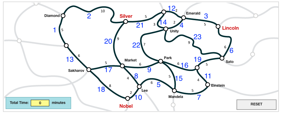
We use the “Traffic” item from PISA 2012 (OECD 2014b) as a motivational example to illustrate various concepts and notation. This item is publicly available online at “http://www.oecd.org/pisa/test-2012/testquestions/question1/”. PISA is a worldwide assessment to evaluate educational performances of different countries and economies. The “Traffic” item contains three questions where the most challenging one asks the examinee to operate on a computer to complete the task, i.e., to locate a meeting point which is within 15 minutes away from three places, Silver, Lincoln and Nobel. There are two correct answers, “Park” and “Silver” for this task. Figure 1 shows the initial state of the computer screen. There are 16 destinations and 23 roads in the map. The integer in blue next to each road is the road number and the integer in black is the traveling time from one end to the other. The examinee could click a road to highlight it, re-click a clicked road to unhighlight, and use “RESET” button to remove all highlighted roads. The “Total Time” box shows the time for traveling on the highlighted roads. Once a road is clicked, the corresponding time would be added to this box. Each action and its corresponding time are sequentially saved in the log file during the process of completing the item. A typical example of the action process of one specific examinee and its cleaned version are shown in Tables 1 and 2. In this case, . After removing unneeded rows (“START_ITEM”, “END_ITEM”, “Click”, “SELECT”), we can see that there are 16 meaningful actions performed by this examinee as listed in Table 2. His/her observed data are
| event_number | event | time | event_value |
| 1 | START_ITEM | 0.00 | NULL |
| 2 | click | 24.60 | paragraph01 |
| 3 | ACER_EVENT | 27.70 | 00000000010000000000000 |
| 4 | click | 27.70 | hit_NobelLee |
| 5 | ACER_EVENT | 28.60 | 00000001010000000000000 |
| 6 | click | 28.60 | hit_MarketLee |
| 7 | ACER_EVENT | 29.40 | 00000001110000000000000 |
| 8 | click | 29.40 | hit_MarketPark |
| 9 | ACER_EVENT | 30.50 | 00000001110000000001000 |
| … | … | … | … |
| 29 | ACER_EVENT | 46.00 | 00110000100000000001010 |
| 30 | click | 46.00 | hit_MarketPark |
| 31 | ACER_EVENT | 47.70 | 00110001100000000001010 |
| 32 | click | 47.70 | hit_MarketLee |
| 33 | ACER_EVENT | 48.70 | 00110001110000000001010 |
| 34 | click | 48.70 | hit_NobelLee |
| 35 | Q3_SELECT | 54.70 | Park |
| 36 | END_ITEM | 66.20 | NULL |
| event_number | time | event type |
| 1 | 27.70 | 10 |
| 2 | 28.60 | 8 |
| 3 | 29.40 | 9 |
| … | … | … |
| 14 | 46.00 | 9 |
| 15 | 47.70 | 8 |
| 16 | 48.70 | 10 |
As seen in the above example, process data are more complicated and also more informative compared with the classical item response data. Different examinees may solve the item using different strategies and with different speeds that can only be seen from the response processes/process data, not the final answers/responses. The form of process data is nonstandard in that action sequences for different examinees are not synchronized and have different lengths. By extracting examinees’ event patterns, including event co-occurrence and time heterogeneity, we can learn their problem-solving strategies and, consequently, better understand the underlying complex problem-solving (CPS) item. With these in mind, we introduce our new model in the next section.
3 Latent Theme Dictionary Model
In this section, we propose a latent theme dictionary model (LTDM). We treat the whole event process of an examinee as a sequence of sentences where each sentence is an ordered subsequence of events. Our proposed model focuses on modeling the event relationships within a sentence. By doing this, we effectively reduce raw data length by splitting the original long sequence to multiple shorter sentences. This way of complexity reduction enables us to model sentences instead of the whole process which is more complicated. We also want to point out that how to split the original event sequence to the sequence of event sentences is case-dependent which can be determined by the expert knowledge. Some special events (e.g. “Reset” action) can be used to split event sequences in general.
To be precise, we assume that and are divided into sentence sequences, i.e. and , where
are called event sentence and time sentence, respectively. We use to represent an ordered pattern that events appear sequentially and call it -gram (length of this pattern is ). Because a 1-gram pattern is also an event, will be used both for event and 1-gram pattern throughout the sequel. Event sentence can be represented as a sequence of patterns,
where is the number of patterns that contains. Note that an event sentence can be partitioned into different pattern sequences. We use to denote the set of all possible pattern separations for . We let be the number of different event patterns of length . We define pattern dictionary as the set of all distinct patterns and use to denote its cardinality, i.e. the size of the dictionary. Obviously, , where is the maximum length of patterns. Next we use “Traffic” item as an example to illustrate the relation between event sentences and event separations.
Example 1
Consider an examinee taking the following actions to complete the “Traffic” item,
We split this observed event sequence to several sentences by using the following criteria. We treat a sentence as a subsequence of actions of consecutively highlighting/unhighlighting the road. In this case, we have a total of three sentences,
Suppose the underlying dictionary is
Then, according to this dictionary, we have
We now specify the probability structure of our proposed model. On a very high level, the proposed model is motivated by two simpler models, latent class model (Gibson 1959, LCM;) and theme dictionary model (Deng et al. 2014, TDM;); see Appendix E for their definitions. Suppose that the entire population consists of different classes of examinees, but their class labels are unknown. We use to denote the latent class to which the examinee belongs. Latent variable can be viewed as the examinee’s latent attribute or discretized version of latent ability. In order to jointly model and , it is equivalent to model and where
| (1) |
with , for , and for . We make the usual local independence assumption, i.e.,
| (2) |
This leads to
| (3) |
where is the probability mass for the th latent class. Thus the sentences are exchangeable.
Next we model event sentence and time sentence by making use of the following conditional probability formula,
| (4) |
For the event part, notice that each observed event sentence may have different pattern separations (i.e. two different pattern sequences can lead to the same event sequence). Thus
| (5) |
We further assume
| (6) |
where and is the number of patterns in . Here (6) is analogous to (A30) in the TDM setting. It specifies that an examinee from latent class has event pattern with probability . The extra term comes from the fact that we consider the pattern orders.
For modeling , we assume
| (7) |
where is the length of . In other words, the gap time between two consecutive events is assumed to be stationary given the latent class label.
From (4) - (7) and the fact that , we have
| (8) |
Finally, we specify that gap time follows an exponential distribution, i.e.,
| (9) |
Different from traditional response time model (van der Linden 2006) where only the total time spent on an item is considered, the proposed model accounts for the time allocated to each action. Here gap time is assumed to follow the exponential distribution while the log-normal assumption is made in classical response time model. Variable can be viewed as the personal intensity. Such modeling often appears in the literature of event history analysis and survival analysis (Allison 1984; Aalen et al. 2008). Here we assume that only depends on the latent class label. In general, it could be individual-specific which is related to the frailty model (Duchateau and Janssen 2007). It could also be event-dependent which is known as the competing risk analysis in the survival analysis. Chen 2019’s dynamic choice model considers the intensity function with both individual effect and event task effect.
Lastly, we assume that , which is the number of sentences for the subject, follows some distribution function supported on , i.e.,
| (10) |
For simplicity, we may assume is a cumulative distribution function of Poisson random variable with parameter . Note that instead of directly modeling , we can also fit the proposed model conditioning on s. This will not effect the estimates of other model parameters.
To summarize, LTDM is a data-driven model that can be used for learning event patterns and population clustering simultaneously. The model framework is built on a very general level in the sense that (1) by letting number of latent classes be 1, the model reduces to TDM-type model with an ordered pattern dictionary and (2) it reduces to a model for event sentences only if we let be constant across all latent classes (i.e. ).
One important set of parameters, , measures how often examinees from different classes use distinct patterns. Another set of parameters, , measures how fast examinees take actions across different groups. In other words, the population are stratified by two factors, event pattern and respond speed. From the information theory viewpoint, we can write
| (11) |
and
| (12) |
where is the Fisher information with respect to a generic parameter for some random vector and is the conditional Fisher information of for some generic random vector given random vector . In particular, taking to be event pattern parameters, , we know that . According to Proposition 1 in Appendix B, the equality is achieved if and only if . This implies that we can estimate event parameter more accurately by observing when response speed are different across different groups. Therefore, the inclusion of event times does not only characterizes the response speed of examinees from different classes but also improves the estimation accuracy of model parameters.
We now construct the likelihood function for LTDM. We use to denote the total number of examinees and subscript to denote the -th examinee. Assume that examinees are independent of each other. Then the complete likelihood of has the following expression,
where . Furthermore, by summing over/integrating out the unobserved latent variables, we have
| (13) | |||||
4 Identifiability
Latent class models (LCMs) often face the issue of identifiability. There is an existing literature on identifiability of latent variable models; see Allman et al. 2009, Xu et al. 2017, and references therein. Theme dictionary model also has the identifiability issue since the underlying separations are unobserved. In this section, we address the identifiability issue, specifically towards dictionary and model parameters in the proposed model. Intuitively, the dictionary and model parameters can be identified if the examinees from different classes have distinct behaviors. To be more specific, two examinees may have different speeds to solve the item and their strategies (event patterns) should be different. In the following, we mathematically investigate this problem and identify the conditions under which the model becomes identifiable.
We use to denote the set of all possible sentences generated by , that is, where is the set of sentences generated by the pattern set of Class , . We define the set
where and . We use to denote an LTDM which depends on . In the sequel, we will omit and use when there is no ambiguity.
We say classes and are equivalent if . We define the set of equivalence classes as . Let be the pattern dictionary of equivalence class and be the set of all possible sentences generated by .
- A1
For any class and any event , it holds that if contains a subsentence with consecutive events in set . Here is the length of longest sentence in without .
- A2
For every pattern in dictionary , are distinct if .
Assumption A1 is a technical condition to ensure that the patterns from distinct classes could be identified. This assumption is satisfied automatically in many cases such as (1) entries of are different or (2) for all . Assumption A2 essentially restricts the dictionary in such a way that each pattern consists of distinct events. Clearly it is very easy to check. It is also natural in the sense that we do not want to treat too many replicated events as a pattern. For example, if we have two dictionaries and , then they would generate the same sentence set (i.e., ). Thus Assumption is necessary for dictionary identifiability. We now introduce the formal definition of identifiability for LTDM.
Definition 1
We say , is identifiable, if for any that satisfies
for all and , and , , we must have
Here we use superscript to denote the true model (parameters/dictionary). means equals up to a permutation of class labels.
We want to point out that in general is too large to be identifiable without additional constraints. It is thus worth specifying a restricted space such that every model dictionary and parameter in is identifiable. Given Conditions C1 and C2 as specified in Appendix A, we define
We have the following theorem.
Theorem 1
Under Conditions C1 and C2, every in is identifiable.
One immediate result as stated in Corollary 1 is that there are no two distinct dictionaries which have the same if they satisfy Assumption A2. This also serves as a sufficient condition for the identifiability of TDMs, since a TDM could be non-identifiable without any additional assumption.
Corollary 1
For the 1-class case, if and satisfy Condition A2, then if and only if .
Suppose that the number of latent classes and dictionary size are known. The true dictionary and model parameters can be estimated consistently. The results are stated as follow.
Theorem 2
Define the maximum likelihood estimator
where ; is the set of dictionaries with size smaller than and is any compact subset containing the true parameter vector. Then, under Conditions C1 and C2, we have that
and, for some permutation function ,
for any as .
We would like to point out that if we only consider the event sentences and ignore the times, the above results still hold since all classes are in a single equivalence class.
5 Computation
Although LTDM postulates a parametric form, we do not know the size of the true dictionary () and the number of latent classes () in practice. Therefore, three challenges remain in terms of computation, namely, (1) finding the true underlying patterns (construction of dictionary), (2) clustering people into the right groups, and (3) computational complexity. We propose a new nonparametric Bayes - LTDM (NB-LTDM) algorithm as described below to address these issues.
-
NB-LTDM Algorithm
-
Initialization: Randomly choose a large ; sample personal latent labels from the uniform distribution on ; sample parameters uniformly on [0,1]; sample from the Dirichlet distribution; sample and from . The initial dictionary should include all 1-grams and a random selection of -grams ().
-
Output: - the number of classes, - the dictionary, estimates of model parameters.
-
The algorithm takes the following iterative steps until the Markov chain becomes stable.
- 1
[Search] Within each latent class, we calculate the frequency of -grams based on count. We find the most frequent -grams () which do not appear in the current dictionary and add them into .
- 2
[Split] Split the event sequences according to the current dictionary.
- 3
[Sample] Sample separation for each event sequence from the corresponding possible candidates.
- 4
[Inner part] Use slice Gibbs (Walker 2007) sampling schemes to iteratively update the following variables:
-
Model parameters and , augmented variables, separations , latent labels and the prior parameters.
-
- 5
[Trim dictionary] For each action pattern in the current dictionary, calculate the evidence probability . Discard those patterns with evidence probability smaller than .
- 1
We set threshold and estimate the number of latent classes by . The estimated pattern dictionary is . We use posterior means for other parameters.
We comment on the tuning parameters in the proposed algorithm: is a threshold to filter out less frequent patterns; is the number of -grams () in the initial dictionary; controls the number of new patterns added into current dictionary. We found in our simulation studies that the proposed method is not sensitive to the choices of and . In practice, we may choose and .
This data-driven method consists of two main steps, updating the dictionary and updating the model parameters.
-
Update dictionary: In each loop, the algorithm trims the dictionary by keeping patterns with high evidence level and discarding those with weak signals. Then it finds patterns (2-grams, …, -grams) with high frequencies within each latent class and adds new patterns to the current dictionary. This step can be viewed as a forward-backward-type variable selection (Tibshirani 1997; Borboudakis and Tsamardinos 2019) technique for dictionary update. Compared with the full Bayesian methods (Ishwaran and Rao 2003; Ishwaran and Rao 2005, e.g. spike-and-slab prior;) for dictionary selection, it can result in substantial reduction in the computational time.
-
Update parameters: To update the model parameters, we follow the approach of Dunson and Xing 2009. In our specific setting, for a given dictionary, the parameters are updated using a Markov Chain Monte Carlo (MCMC) method together with the slice sampler. It allows us to avoid directly computing the marginal likelihood that requires massive computation in terms of integration of latent variables and . We use a stick-breaking prior (Sethuraman 1994) on latent class probabilities to avoid specifying a priori number of classes . For precise mathematical formulation and updating rules in the inner part, see Appendix C.
Here we want to point out that we are not able to develop theoretical results for convergence analysis. However, the proposed method performs well in our simulation studies.
6 Simulation Studies
The simulation studies include four different simulation settings, which are specified below.
- 1.
In the first simulation setting, dictionary consists of -grams, -grams and -grams, with details given in Table 3. We set , , and set , . Other model parameters are set as follow, , and . Pattern probability is provided in Table 3.
=========================
Insert Table 3 about here
=========================
Under this setting, it can be verified that the model dictionary and parameters are identifiable: A1 is satisfied since ’s are different; A2 holds by the construction of dictionary; C1 and C2 are satisfied as the size of each equivalence class is 1.
- 2.
In the second simulation setting, dictionary consists of -grams, -grams and -grams, with details given in Table 4. We set , , and set , . Other model parameters are set as follows, , and . Pattern probability is provided in Table 4.
=========================
Insert Table 4 about here
=========================
Under this setting, the model dictionary and parameters are identifiable. It is easy to see that there are four equivalence classes, , , and where and . Assumption A1 is satisfied by observing that pattern dictionaries of Class 1 (2) and Class 3 (4) do not overlap. Assumption A2 holds by the construction of dictionary. We can construct a partition such that sentence has only one separation for any (). It can be checked directly that the corresponding -matrices have full column rank. Therefore C1 is satisfied. Condition C2 can also be verified similarly.
- 3.
In the third simulation setting, dictionary includes patterns up to -grams, with details provided in Table 5. We let , , and set , . Other model parameters are set as follows, , and . Pattern probability is provided in Table 5.
=========================
Insert Table 5 about here
=========================
The model in this setting is also identifiable: A1 is satisfied since ’s are different; A2 holds by noticing that there is no pattern with repeated actions; C1 and C2 are also satisfied automatically since the size of each equivalence class is 1.
- 4.
In the fourth simulation setting, dictionary includes patterns up to -grams, with details provided in Table 6. We let , , and set , . Other model parameters are set as follows, , and . Pattern probability is provided in Table 6.
=========================
Insert Table 6 about here
=========================
The model parameter in this setting is not identifiable: examinnes from Class 1 and Class 2 have almost the same pattern probabilities except for two patterns. Specifically, Class 1 does not have pattern and Class 2 does not have pattern . Therefore, it fails to meet Condition C1. Thus we do not expect that all five classes can be recovered in this setting.
We generate 50 datasets for each setting. To provide a more concrete sense of data, some descriptive statistics are given. The means of sentence length are 6.71, 6.89, 4.88 and 5.02 for Settings 1, 2, 3 and 4 respectively. The maximum lengths of whole event sequences are around 178, 182, 135, 133 for Settings 1, 2, 3 and 4, respectively. The detailed procedures for generating the data sets are presented below.
-
Data Generation Scheme
-
Input: , , , , and .
-
For do
- 1.
Sample from the multinomial distribution with parameter .
- 2.
Sample from the Poisson distribution with parameter .
- 3.
For , do
- –
For each , sample a indicator variable from the Bernoulli distribution with parameter .
- –
Randomly shuffle patterns in set and get an ordered pattern sequence.
- –
Concatenate all patterns in above sequence and get the event sentence .
- –
Compute the length of , i.e., .
- –
Generate recursively, such that for , where and .
- –
- 1.
-
Output: List of event sentences and list of time sentences .
We set threshold for each setting. The performance of proposed model is evaluated through the following criteria.
-
Correct recovery: percent of correctly identified patterns out of all true patterns.
-
False recovery: percent of incorrectly identified patterns out of all identified patterns.
-
-gram hitting: percent of correctly identified -grams out of all true -grams.
-
Class recovery: percent of recovering true number of latent classes.
-
RMSE: Root mean squared error of model parameters.
=========================
Insert Table 7 about here
=========================
=========================
Insert Table 8 about here
=========================
From Table 7, we can see that the proposed method can recover dictionary and model parameters well. The fact that “correct recovery” is close to 1 and “false recovery” is close 0 provides the empirical evidence that is identifiable. The 2-grams, 3-grams are accurately recovered in all three settings. Their hitting rates are all close to 1. The “4-gram hitting” is also high in Setting 3. The estimates of mixing proportion , response speed and pattern probability are close to their true values with small RMSEs. These results provide the supporting evidence on the identifiability of model parameters.
Furthermore, in Settings 1 and 2, we compare the differences between results by fitting the model with/without times. Note that the model in Setting 1 remains estimable if times are ignored. However, from Table 7, we can see the increase in RMSEs of parameters and the decrease in “class recovery” when the times were taken out. This is consistent with the information theoretical results presented in Section 3. In Setting 2, the true number of latent classes is not identifiable when we ignore the times, since Classes 1 and 2 are merged together into a single class, similarly for Classes 3 and 4. The true ’s are no longer estimable for Classes 1-4. In fact, the estimator converges to its average value . These results show that the inclusion of event times can lead to more accurate estimation and better identifiability. From Table 8, under Setting 4, we can see that the proposed algorithm tends to find four classes instead of five classes (i.e. 66 percent of time the algorithm returns a four-class model). The estimate indicates that Class 1 and Class 2 are merged together since we cannot distinguish between them. On the other hand, the underlying dictionary can still be recovered with high accuracy.
From these results, we can see that the proposed algorithm is expected to recover the true latent classes and pattern structures when examinees from different classes have different patterns with different respond speeds.
7 Real Data Analysis
In this section, we apply the proposed model to the “Traffic” item from PISA 2012 as described in Section 2. The data were preprocessed as follows. We removed those examinees who did not answer all three questions of the “Traffic” item or did not take any actions, leaving 10048 remaining examinees. In the raw data, each event corresponding to the map is a 0-1 vector with 23 entries. Note that two consecutive vectors only differed at one position. We took their difference and represented event as the index on which the two consecutive vectors differ. We view highlighting and unhighlighting as two different knowledge status of the examinee. As such, a sentence was defined as a subsequence of events where the examinee either consecutively highlighted roads or consecutively unhighlighted roads. A new sentence starts once the examinee changed from highlighting (unhighlighting) to unhighlighting (highlighting), or clicked “reset”. The corresponding time sentence was defined accordingly. An example of such data transformation is shown in Table 2. In our case, the observed data is and . The corresponding observed event and time sentence sequences are and . On average, each individual had about 10.4 sentences and clicked around 28.4 roads.
To apply the proposed method, we set and by observing that the correct meeting point is at most three roads away from each place marked in red. Six classes were identified with the LTDM and were labeled in descending order according to their sizes. Table 9 provides a summary, such as mixing proportion, answer correct rate, average number of sentences (actions), etc., for the six classes. The size of estimated dictionary was 82 with , and ; see Appendix D for details.
=========================
Insert Table 9 about here
=========================
The fitted model appeared to satisfy the required assumptions and conditions. Assumption A1 was satisfied since the size of each equivalence was one by noticing that ’s were significantly different from each other. Assumption A2 was satisfied by observing that no pattern had repeated events. Conditions C1 and C2 also held since the size of each equivalence class was one.
From Table 9, we can see that there was a substantial variation among the estimated intensities . Classes 2 and 3 had the highest response speed and the highest correct rate. The examinees from Class 6 responded much slower compared to other classes but still had a decent chance to get the correct answer. It shows that they made efforts to solve this CPS item. Examinees from Classes 4 and 5 solved the item with moderate speed. They had the lowest chance to get the correct answer. The results indicate that the time information may be useful in characterizing examinees.
=========================
Insert Table 10 about here
=========================
We next look at the most frequent patterns (2-grams, 3-grams) in Table 10. Examinees in Classes 2 and 3 had a much higher chance to solve the item. They could successfully identify three paths connecting the correct meeting point “Park” to three original places, “Silver”, “Nobel” and “Lincoln”. Note that there are two paths connecting “Silver” and “Park” with less than 15 minutes, i.e. and . Examinees in Class 3 identified the former path and Examinees in Class 2 identified the latter. Pattern is shorter, thus Class 3 was the most efficient class. Examinees in Class 4 barely used any most frequent 2-gram or 3-gram patterns. They did not appear to have a good strategy that led to a lower rate of solving the item successfully. Examinees from Class 5 behaved differently from other classes. They identified paths connecting “Silver” to “Lincoln” or “Nobel” , i.e., , , and . In other words, these examinees found the second correct meeting point “Silver”. But unfortunately, most of them failed to identify “Park”. Hence, they have the lowest rate to answer the item correctly. Examinees from Class 1 or Class 6 tended to have patterns such as , , . These patterns were partial paths from three original places to the correct meeting point “Park”. This explains that Examinees in these two classes had a moderate chance to answer the question correctly.
To summarize, the proposed approach produces a useful model and classifies examinees into interpretable classes. The results suggest that an efficient examinee (i.e. fewer actions, higher usage of frequent patterns) was more likely to successfully complete the task. Since “Traffic” item tests the ability of “Exploring and understanding” and “Planning and executing” (OECD 2014a), our results suggest that this item achieved what it was intended for.
8 Discussion
In this paper, we proposed a new statistical model, the latent theme dictionary model, to deal with the process data and developed the NB-LTDM algorithm. The new approach allows us to extract co-occurrent patterns and to classify individuals automatically based on data without pre-specifying the dictionary and the number of classes. In addition, we established the theoretical properties of the proposed method, including model identifiability and consistency of parameter estimation. The simulation results confirmed the theoretical findings. We also applied the new method to the 2012 PISA “Traffic” item and obtained meaningful results.
It is easy to incorporate domain knowledge into our approach. If certain patterns are selected by experts, we can simply add them to the dictionary. On the other hand, if some patterns are known to be impossible or meaningless, they can be excluded from the dictionary. Because of its generality, the proposed model can be applied in other context such as text mining and speech pattern recognition, where different articles and speeches could be clustered based on their word patterns. It can also be applied in user behavioral studies in e-commerce, online social networking, etc., where users’ frequent daily action patterns can be extracted and user preference database can thus be built.
There are limitations in the proposed method that need to be addressed in further studies. First, although LTDM focuses on finding the ordered event pattern structure within a sentence, we do not have an automated general rule for splitting the original event sequence to a list of sentences. Rather, the current sentence splitting method is ad hoc, relying on expert knowledge. Second, it is an exploratory method to discover the underlying dictionary of action patterns and latent classes of examinees. However, the current algorithm does not have the theoretically guaranteed convergence, though it works well empirically. Third, in the current setting, the response speed only depends on examinee’s latent class membership which may not fully capture the heterogeneity among examinees. A possible approach is to introduce individualized random effects to accommodate such heterogeneity.
References
- Aalen et al. (2008) Aalen, O., Borgan, O. and Gjessing, H. (2008) Survival and event history analysis: a process point of view. Springer Science & Business Media.
- Allison (1984) Allison, P. D. (1984) Event history analysis: Regression for longitudinal event data. No. 46. Sage.
- Allman et al. (2009) Allman, E., Matias, C. and Rhodes, J. (2009) Identifiablity of parameters in latent structure models with many observed variables. The Annals of Statistics, 37, 3099–3132.
- Blei et al. (2003) Blei, D. M., Ng, A. Y. and Jordan, M. I. (2003) Latent dirichlet allocation. Journal of machine Learning research, 3, 993–1022.
- Borboudakis and Tsamardinos (2019) Borboudakis, G. and Tsamardinos, I. (2019) Forward-backward selection with early dropping. The Journal of Machine Learning Research, 20, 276–314.
- Chen (2019) Chen, Y. (2019) A continuous-time dynamic choice measurement model for problem-solving process data. arXiv preprint arXiv:1912.11335.
- Chen et al. (2005) Chen, Y.-L., Tang, K., Shen, R.-J. and Hu, Y.-H. (2005) Market basket analysis in a multiple store environment. Decision support systems, 40, 339–354.
- Deng et al. (2014) Deng, K., Geng, Z. and Liu, J. S. (2014) Association pattern discovery via theme dictionary models. Journal of the Royal Statistical Society: Series B (Statistical Methodology), 76, 319–347.
- Duchateau and Janssen (2007) Duchateau, L. and Janssen, P. (2007) The frailty model. Springer Science & Business Media.
- Dunson and Xing (2009) Dunson, D. B. and Xing, C. (2009) Nonparametric bayes modeling of multivariate categorical data. Journal of the American Statistical Association, 104, 1042–1051.
- Fang et al. (2019) Fang, G., Liu, J. and Ying, Z. (2019) On the identifiability of diagnostic classification models. Psychometrika, 84, 19–40.
- Gibson (1959) Gibson, W. A. (1959) Three multivariate models: Factor analysis, latent structure analysis, and latent profile analysis. Psychometrika, 24, 229–252.
- Goodman (1974) Goodman, L. A. (1974) Exploratory latent structure analysis using both identifiable and unidentifiable models. Biometrika, 61, 215–231.
- Goodman et al. (2013) Goodman, M., Finnegan, R., Mohadjer, L., Krenzke, T. and Hogan, J. (2013) Literacy, Numeracy, and Problem Solving in Technology-Rich Environments among US Adults: Results from the Program for the International Assessment of Adult Competencies 2012. First look (NCES 2014-008). ERIC.
- Griffin et al. (2012) Griffin, P., McGaw, B. and Care, E. (2012) Assessment and Teaching of 21st Century Skills. Springer.
- Han et al. (2019) Han, Z., He, Q. and von Davier, M. (2019) Predictive feature generation and selection using process data from pisa interactive problem-solving items: An application of random forests. Frontiers in Psychology, 10.
- Hastie et al. (2005) Hastie, T., Tibshirani, R., Friedman, J. and Franklin, J. (2005) The elements of statistical learning: data mining, inference and prediction. The Mathematical Intelligencer, 27, 83–85.
- He and von Davier (2016) He, Q. and von Davier, M. (2016) Analyzing process data from problem-solving items with n-grams: Insights from a computer-based large-scale assessment. In Handbook of research on technology tools for real-world skill development, 750–777. IGI Global.
- Ishwaran and Rao (2003) Ishwaran, H. and Rao, J. S. (2003) Detecting differentially expressed genes in microarrays using bayesian model selection. Journal of the American Statistical Association, 98, 438–455.
- Ishwaran and Rao (2005) Ishwaran, H. and Rao, J. S. (2005) Spike and slab variable selection: frequentist and bayesian strategies. The Annals of Statistics, 33, 730–773.
- Kruskal (1977) Kruskal, J. B. (1977) Three-way arrays: rank and uniqueness of trilinear decompositions, with application to arithmetic complexity and statistics. Linear algebra and its applications, 18, 95–138.
- Liu et al. (2012) Liu, J., Xu, G. and Ying, Z. (2012) Data-driven learning of q-matrix. Applied psychological measurement, 36, 548–564.
- Liu et al. (2013) Liu, J., Xu, G. and Ying, Z. (2013) Theory of the self-learning q-matrix. Bernoulli: official journal of the Bernoulli Society for Mathematical Statistics and Probability, 19, 1790.
- Lord (1980) Lord, F. M. (1980) Applications of item response theory to practical testing problems. Routledge.
- OECD (2014a) OECD (2014a) Assessing problem-solving skills in PISA 2012.
- OECD (2014b) OECD (2014b) PISA 2012 technical report. (Available at) http://www.oecd.org/ pisa/pisaproducts/pisa2012technicalreport.htm.
- OECD (2016) OECD (2016) PISA 2015 results in focus. (Available at) https://www.oecd.org/ pisa/pisa-2015-results-in-focus.pdf.
- Piatetsky-Shapiro (1991) Piatetsky-Shapiro, G. (1991) Discovery, analysis, and presentation of strong rules. Knowledge discovery in databases, 229–238.
- Qiao and Jiao (2018) Qiao, X. and Jiao, H. (2018) Data mining techniques in analyzing process data: a didactic. Frontiers in psychology, 9, 2231.
- Sethuraman (1994) Sethuraman, J. (1994) A constructive definition of dirichlet priors. Statistica sinica, 639–650.
- Templin et al. (2010) Templin, J., Henson, R. A. et al. (2010) Diagnostic measurement: Theory, methods, and applications. Guilford Press.
- Tibshirani (1997) Tibshirani, R. (1997) The lasso method for variable selection in the cox model. Statistics in medicine, 16, 385–395.
- van der Linden (2006) van der Linden, W. J. (2006) A lognormal model for response times on test items. Journal of Educational and Behavioral Statistics, 31, 181–204.
- Vermunt and Magidson (2002) Vermunt, J. K. and Magidson, J. (2002) Latent class cluster analysis. Applied latent class analysis, 11, 89–106.
- Walker (2007) Walker, S. G. (2007) Sampling the dirichlet mixture model with slices. Communications in Statistics—Simulation and Computation®, 36, 45–54.
- Xu et al. (2017) Xu, G. et al. (2017) Identifiability of restricted latent class models with binary responses. The Annals of Statistics, 45, 675–707.
- Xu et al. (2018) Xu, H., Fang, G., Chen, Y., Liu, J. and Ying, Z. (2018) Latent class analysis of recurrent events in problem-solving items. Applied Psychological Measurement.
- Xu et al. (2019) Xu, H., Fang, G. and Ying, Z. (2019) A latent topic model with markovian transition for process data. arXiv preprint arXiv:1911.01583.
Appendix A: Conditions C1 and C2
We provide the exact statements of conditions C1 - C2 in this appendix.
- C1.a
For each equivalence class with size larger than 1, there exists a partition of 1-grams such that for any , and , sentence and sentence admit only one separation. Cardinalities of three sets satisfy , and . Here is the cardinality of equivalence class .
- C1.b
Define -matrices , and such that for , , and . Matrices , and have full column rank.
- C2.a
For each equivalence class with size larger than 1 and for any -gram with , there exists (the subset of 1-grams) such that (1) for any , sentence does not admit other separations containing -gram or -gram other than ; (2) cardinality of is greater than or equal to .
- C2.b
Define matrix such that for and . Matrix has full column rank.
Conditions C1 - C2 pertain to the dictionary and parameter structures. Specifically, Condition C1.a puts the restrictions on 1-grams such that not all combinations of 1-grams are considered as patterns, which ensures the pattern frequency can be identified. It is very similar to the sufficient conditions in identifiability of diagnostic classification models (Xu et al. 2017; Fang et al. 2019, DCMs,), where they require all items can be divided into three non-overlapping item sets. Here 1-gram can be viewed as the counterpart of item in DCMs. Condition C2.a requires that each -gram is not overlapped with other patterns to some extent and thus can be identified. Conditions C1.b and C2.b require that the examinees from different groups should have different pattern frequencies.
The -matrices here share the similar ideas to those in Liu et al. 2012; Liu et al. 2013. We use the following example to illustrate this idea.
Example 2
Consider a 2-class model with and . Pattern probability is
Appendix B: Proofs
To prove main theoretical results, we start with two lemmas which play key roles for dictionary and parameter identifiability. The proof of Lemma 2 is presented at the end of this section.
Lemma 1 (Kruskal 1977)
Suppose are six matrices with columns. There exist integers , , and such that . In addition, every columns of are linearly independent, every columns of are linearly independent, and every columns of are linearly independent. Define a triple product to be a three-way array where . Suppose that the following two triple products are equal . Then, there exists a column permutation matrix such that , where are diagonal matrices and identity. Column permutation matrix is right-multiplied to a given matrix to permute the columns of that matrix.
Lemma 2
Under Assumptions A1 and A2, it holds that if and only if .
Here we recall that is the observed sentence set generated from equivalence class and is the dictionary consisting of patterns from equivalence class .
- Proof of Theorem 1.
For every model , we need to show that if there exists another model such that
it must hold .
We prove it through the following steps. (1) -identifiability: we show that the parameter is identifiable. (2) -identifiability: we prove that for any equivalence class . (3) Dictionary identifiability: we show that implies . (4) -identifiability: we show that and .
For -identifiability, we can see that the marginal distribution of and is
(A2) By taking , we have that . Then it must hold that
This implies that .
For -identifiability, we consider take and an event sentence and . Then, ( Proof of Theorem 1.) becomes
By -identifiability, we further have
(A4) after simplification. Let , we must have that , where is the equivalence class with minimum lambda value. Hence, we also have . Then (A4) becomes
By the similar strategy, we can show that for every equivalence class . This gives -identifiability.
For the dictionary identifiability, we would like to point out that its proof is not covered in Deng et al. 2014. Therefore, we seek an alternative approach to prove it.
By taking , an arbitrary sentence and where is the sentence length. Then ( Proof of Theorem 1.) becomes
Comparing the coefficients on both sides of ( Proof of Theorem 1.), we then have
(A6) This implies that . By Lemma 2, we then have . Notice that . It concludes the dictionary identifiability.
For -identifiability, we prove it by making use of (A6). In (A6), we take for , with from different partition sets, and with , sequentially.
Without loss of generality, we suppose there is only one equivalence class. According to Condition C1.a that only admits one separation, (A6) can be simplified as
if (A7) if (A8) (A9) where we define , . In addition, if we take to be an empty sentence, then it holds
(A10) It is not hard to write equations (A7) - (A10) in terms of tensor products of matrices, that is,
where
and
Here, is a by diagonal matrix with its -th element equal to . By Condition C1.b, column ranks of matrix , and are full column rank. Therefore, by Lemma 1, we have that
where matrix is a column permutation matrix, and are diagonal matrices satisfying . Since elements in first rows of are all ones, it implies . Therefore, as well. Thus, we have , and . By comparing element-wisely, we can see that and up to a label switch. Further, due to the monotonicity relation between and .
In the following, we prove that is identifiable up to the same label switch for any pattern by induction. Suppose we have that is generically identifiable when belongs to {1-grams, …, (-1)-grams}. We need to show that is identifiable if is a -gram.
Let be the sentence set including all -grams in and all possible combinations of -gram and -gram that are not in . It is not hard to see that for each , its separation can only be the combinations of all -grams () or the combinations of gram and -gram.
if and is -gram; if , is a -gram and ; By previous results that and for those ’s are 1-grams, we could write above equations in the following matrix form, that is,
(A11) where and
Here, are distinct 1-grams in . According to Condition C2.a and C2.b, (A11) admits only one solution. Therefore, , which implies . Hence, we conclude that up to a label switch for all . This concludes the -identifiability. By completing all steps, we establish the identifiability results.
- Proof of Theorem 2.
We prove this result by two steps. In Step 1, we prove that dictionary can be estimated consistently. In Step 2, we show that the estimator, , is consistent. Without loss of generality, we take compact set as = {, }, where , , are some positive constants such that true model parameter is in .
Proof of Step 1 We first introduce several useful event sets. Define an event set ,
(A12) In other words, all possible sentences are at least observed once on . Define sets , , and . Next we show that holds with high probability. Specifically, we show the upper bound for by decomposing into four parts, i.e.,
- 1..
By large deviation property of Poisson random variable , we have that where .
- 2..
It is not hard to see that for some constant by using Poisson moment generating function.
- 3..
By union bound, we can get that . Here is the longest sentence length and .
- 4..
We show that has a positive lower bound for every sentence . Take an arbitrary , we know that . Hence for and such that . Thus is bounded below by , i.e., .
Therefore, we have that .
Hence, event holds with probability at most .
On event , we have that all sentence in are at least observed once. By the dictionary identifiability from Theorem 1, we know that . In other words, . This completes Step 1 by choosing and .
Proof of Step 2 For any fixed parameter . Let denote the log-likelihood evaluated at . By identifiability we know that, for any distinct . By compactness of and continuity of (see (A19)), there exists a positive number such that for any . In next, we prove the uniform convergence of to the expected value.
By Bernstein inequality, we know that
(A13) holds point-wisely. By compactness, is bounded by some constant . Thus
(A14) for any fixed .
Next, we consider bound the gap between . For notational simplicity, we omit subscript in the following displays. We know that
(A15) For , we can see that for some constant . We can further show that and on set . This is because
(A16) and
(A17) With (A16) and (A17), (A15) becomes
(A18) by adjusting the constant.
Next we prove that is a continuous function of . Define set for . By algebraic calculation, for any with , we have
(A19) by adjusting the constant.
- 1..
Proposition 1
Under LTDM setting, the probability mass function can be written in the multiplicative form of if and only if . Here is the model parameter excluding , and are some functions.
- Proof of Proposition 1.
First, we write out the likelihood function
(A24) where is some quantity depending on and .
We first prove the sufficient part. Suppose . Then (A24) can be written as
(A25) (A26) Hence we can take and . This concludes the sufficient part.
We next prove the necessary part. Suppose it is not true. In other words, we can write when ’s are not all the same. Without loss of generality, we assume . By assumption,
(A27) Divided by on both sides of (A27), we get
(A28) By letting , the left hand side of (A28) becomes . Then we know that has the form of . Plug this back to (A27), we then get
Notice that the left hand side of above equation is a polynomial of ’s and right hand side is a polynomial of ’s. Hence it must hold that for , which is impossible when . Thus it contradicts with the assumption. This concludes the proof of necessary part.
- Proof of Lemma 2.
For any pattern in , we need to show it also belongs to . It is easy to see that if has the form of , then it must belong to since only admits one separation. In the following, we only need to consider such that () are different according to Assumption A2. With out loss of generality, we assume belongs to Class .
Let denote the longest sentence generated by satisfying that (1) each event belongs to ; (2) the length of is at least (See ’s definition in Assumption A1). Notice that may not be unique, we only need to consider one of them. Let be the sentence such that it has form such that (1) contains as its subsentence; (2) Each event in belongs to ; (3) is longest possible; (4) The first event of is (Be empty if it does not exist.); (5) is shortest possible. Notice may not be unique, we only need to consider one of them. Next we consider the decomposition of sentence . By aid of , we can show that must belong to .
Since , we know that . Without loss of generality, we also assume that appears in -th class of model . We claim that only has separations in form in . ( is one realization of separation for .) If not, then we must have the following cases.
Case 1: There is a separation such that where is contained in . By Assumption A2, we know that does not consist of . Then, we consider sentence . It is in , then it must in . By Assumption A1, we know that must belong to , since it contains . Then, can be written in form of with longer . This contradicts with the definition of . Therefore, Case 1 cannot happen.
Case 2: There is a separation such that where contains . We further consider the following four situations.
- 2.a.
Suppose contains as its sub-sentence and does not contain events . Since , we know that must belong to . By Assumption A1, is also in . Then, it leads to contradiction since is longer than .
- 2.b.
Suppose contains as its sub-sentence and contains events . is also in for the same reason as before. This time, can be written in the form of with shorter , which contradicts with the definition of .
- 2.c.
Suppose is contained in . If is the longest sentence generated by without , then by Assumption A1 we know must also belong to this class. Therefore, is not the longest sentence. It implies that there exists a pattern with events in in does not contribute to . Therefore, sentence containing must belong to . By using the same argument, we know that it can also be written in the form with longer . This contradicts with the definition of .
- 2.d.
Suppose . If is not empty, then contains two ’s. It contradicts with Assumption A2. If is empty, then exactly.
Hence, we conclude the proof of this lemma.
- 2.a.
Appendix C: Parameter Estimation in NB-LTDM
In the inner part of the NB-LTDM Algorithm, we adopt a nonparametric Bayes method which is used to avoid selection of a single finite number of mixtures . Therefore, we replace finite mixture components by an infinite mixture, that is,
For the choice of prior, we specify , , and where corresponds to a Dirichlet process. The stick-breaking representation, introduced by Sethuraman 1994, implies that with independently for , where is a precision parameter characterizing .
Hence, our nonparametric Bayesian latent theme dictionary model can be written in the following hierarchical form:
where is the Dirac measure at .
We use a data augmentation Gibbs sampler (Walker 2007) to update all parameters and latent variables. Specifically, we introduce a vector of latent variables , where . The full likelihood becomes
where is the density of , is the density of and is the density of .
Then Gibbs sampler iterates through the following steps:
- 1.
Update , for , by sampling from .
- 2.
Update , for , by sampling from
- 3.
Update , for (), by sampling from
- 4.
Update , for , by sampling from truncated to fall into the interval
- 5.
Update , for , by sampling from
where . To identify the elements in , first update for , where is the smallest value satisfying
(A29) Therefore, are the possible values for . Note that we have already updated for . Therefore, we first check if satisfies (A29). If yes, then we do not have to sample more; otherwise sample for until (A29) is satisfied. In this case, we also have to sample from and from for and in order to compute for .
- 6.
Update , for , , by sampling from
- 7.
Update , which follows gamma distribution .
- 8.
Sample from posterior .
Appendix D: Estimated Dictionary in Traffic Item
In the “Traffic” item, the NB-LTDM algorithm found a dictionary with . For each pattern in , we classified the six classes into two clusters based on their pattern probabilities . Those classes with high pattern probabilities are clustered together and shown in Table 11.
=========================
Insert Table 11 about here
=========================
Appendix E: Latent Class Model and Theme Dictionary Model
In this section, we briefly recall two popular models, latent class model (Gibson 1959, LCM;) and theme dictionary model (Deng et al. 2014, TDM;), which are related with the proposed LTDM.
Widely adopted in biostatistics, psychometrics and machine learning literature (Goodman 1974; Vermunt and Magidson 2002; Templin et al. 2010, e.g.,), LCM relates a set of observed variables to a discrete latent variable, which is often used for indicating the class label. LCM assumes a local independence structure, i.e.,
where are observed variables and is a discrete latent variable with density . Thus, the joint (marginal) distribution of takes form
For TDM (Deng et al. 2014), it typically handles observations known as words/events. It can be used for identifying associated event patterns. The problem of finding event associations is also known as market basket analysis (Piatetsky-Shapiro 1991; Hastie et al. 2005; Chen et al. 2005). Under TDM, a pattern is a combination of several events. A collection of distinct patterns forms a dictionary, . An observation, , is a set of events. In TDM, we observe but do not know which patterns it consists of. In other words, could be split into different possible partitions of patterns. For each possible partition, we call it a separation of . The collection of multiple observations forms a document. TDM does not take into account event ordering. For example, is an observation with three events, , and . TDM treats as the same observation as . Consequently, patterns are also unordered. For instance, patterns and are viewed as the same. TDM postulates that a pattern appears in an observation at most once. Let be the probability of pattern that appears in an observation. The probability distribution of one separation for observation is defined to be
| (A30) |
Since separation is not observed, the marginal probability of is
where is the set of all possible separations for . Furthermore, observations are assumed to be independent, i.e., for ,
1-10: 1-gram 11-20: 1-gram 21-30: 2-gram 31-40: 2-gram 41-45: 3-gram 46-50: 3-gram 1 0.3 0 0.2 0 0 0 2 0 0.3 0 0.2 0 0 3 0.2 0.2 0.05 0.05 0.001 0.001 4 0.05 0.05 0 0 0.3 0 5 0 0 0.03 0.03 0 0.3
Specification of dictionary 1-grams (1-20) [1], [2], …, [20] 2-grams (21 - 30) [1 2], [2 3], [3 4], [4 5], [5 1], [6 7], [7 8], [8 9], [9 10], [10 6] 2-grams (31 - 40) [11 12], [12 13], [13 14], [14 15], [15 11], [16 17], [17 18], [18 19], [19 20], [20 11] 3-grams (41 - 45) [11 12 14], [12 13 15], [13 14 12], [14 15 11], [15 11 13] 3-grams (46 - 50) [1 2 4], [2 3 5], [3 4 7], [3 9 6], [2 5 6]
1-10: 1-gram 11-20: 1-gram 21-30: 2-gram 31-40: 2-gram 41-45: 3-gram 46-50: 3-gram 1 0.3 0 0.2 0 0 0 2 0.3 0 0.2 0 0 0 3 0 0.3 0 0.2 0 0 4 0 0.3 0 0.2 0 0 5 0.05 0.05 0 0 0.3 0 6 0 0 0.03 0.03 0 0.3
Specification of dictionary 1-grams (1-20) [1], [2], …, [20] 2-grams (21 - 30) [1 2], [2 3], [3 4], [4 5], [5 1], [6 7], [7 8], [8 9], [9 10], [10 6] 2-grams (31 - 40) [11 12], [12 13], [13 14], [14 15], [15 11], [16 17], [17 18], [18 19], [19 20], [20 11] 3-grams (41 - 50) [1 2 4], [2 3 5], [3 4 7], [3 9 6], [2 5 6] 3-grams (46 - 50) [11 12 14], [12 13 15], [13 14 12], [14 15 11], [15 11 13]
1-15: 1-gm 15-30: 1-gm 31-35: 2-gm 36-50: 2-gm 50-60: 2-gm 61-70: 3-gm 71-75: 3-gm 76-85: 4-gm 86-90: 4-gm 1 0.15 0 0 0 0 0.06 0.06 0 0 2 0 0.15 0.06 0.06 0.06 0 0 0 0 3 0.05 0.05 0.05 0.001 0.001 0.05 0.001 0.001 0.001 4 0 0 0.03 0.03 0 0 0 0.05 0 5 0.04 0.04 0 0 0 0 0 0 0.1
Specification of dictionary 1-grams (1-30) [1], [2], …, [30] 2-grams (31 - 45) [1 2], [2 1], [2 3], [3 2], [3 4], [4 3], [4 5], [5 4], [5 1], [1,5], [6 7], [7 8], [8 9], [9 10], [10 6] 2-grams (46 - 60) [11 12], [12 13], [13 14], [14 15], [15 11], [16 17], [17 18], [18 19], [19 20], [20 11], [1 11], [2 12], [3 13], [4 14], [5 15] 3-grams (61 - 68) [1 2 4], [2 3 5], [3 4 7], [3 9 6], [2 5 6], [2 1 4], [3 2 5], [4 2 7] 3-grams (69 - 75) [11 12 14], [12 13 15], [13 14 12], [14 15 11], [15 11 13], [12 11 14], [13 12 15] 4-grams (76 - 83) [1 2 3 4], [2 3 5 1], [3 4 7 1], [3 9 6 2], [2 5 6 4], [3 4 1 2], [5 1 7 8], [6 9 3 4] 4-grams (84 - 90) [11 12 13 14], [12 13 15 11], [13 14 17 11], [24 25 26 27], [24 26 28 30], [11 16 21 26], [16 11 26 21]
1-10: 1-gram 11-20: 1-gram 21-30: 2-gram 31-40: 2-gram 41-45: 3-gram 46-50: 3-gram 1 0.15 0.15 0.1(except 21) 0 0 0 2 0.15 0.15 0.1(except 22) 0 0 0 3 0.1 0.1 0 0.15 0.0 0.0 4 0.05 0.05 0 0 0.3 0 5 0 0 0.03 0.03 0 0.3
Specification of dictionary 1-grams (1-20) [1], [2], …, [20] 2-grams (21 - 30) [1 2], [2 3], [3 4], [4 5], [5 1], [6 7], [7 8], [8 9], [9 10], [10 6] 2-grams (31 - 40) [11 12], [12 13], [13 14], [14 15], [15 11], [16 17], [17 18], [18 19], [19 20], [20 11] 3-grams (41 - 45) [11 12 14], [12 13 15], [13 14 12], [14 15 11], [15 11 13] 3-grams (46 - 50) [1 2 4], [2 3 5], [3 4 7], [3 9 6], [2 5 6]
Setting 1 Correct recovery % False recovery % 2-gram hitting 3-gram hitting Class recovery No time 99.6 % 0.3 % 100.0 % 98.8% 84 % With time 99.9 % 0.1 % 100.0 % 99.6% 94 % C1 C2 C3 C4 C5 No time 0.40 0.298 0.199 0.053 0.049 RMSE 0.015 0.014 0.014 0.007 0.007 With time 0.399 0.299 0.202 0.049 0.051 RMSE 0.016 0.013 0.014 0.006 0.007 No time 9.99 2.50 1.00 0.497 0.200 RMSE 0.080 0.026 0.014 0.013 0.005 With time 10.0 2.50 0.999 0.501 0.201 RMSE 0.072 0.024 0.014 0.012 0.005
Setting 2 Correct recovery % False recovery % 2-gram hitting 3-gram hitting Class recovery Reduced recovery No time 96.6 % 3.5 % 100.0 % 89.6% 0 % 92 % With time 97.3 % 2.7 % 100.0 % 91.8% 98 % - C1 C2 C3 C4 C5 C6 No time 0.396 - 0.402 - 0.102 0.100 RMSE 0.018 - 0.016 - 0.009 0.008 With time 0.201 0.198 0.201 0.201 0.099 0.100 RMSE 0.012 0.014 0.012 0.012 0.008 0.009 No time 0.378 - 0.380 - 0.997 0.999 RMSE 0.017 - 0.016 - 0.017 0.020 With time 0.200 4.01 0.200 0.201 1.00 1.00 RMSE 0.002 0.043 0.002 0.046 0.017 0.019
Setting 3 Correct recovery % False recovery % 2-gram hitting 3-gram hitting 4-gram hitting Class recovery With time 98.9 % 1.4 % 100.0 % 99.0% 96.3 % 98 % C1 C2 C3 C4 C5 With time 0.303 0.298 0.201 0.099 0.100 RMSE 0.010 0.010 0.009 0.007 0.007 With time 9.99 2.50 1.00 0.50 0.20 RMSE 0.085 0.017 0.013 0.008 0.003
Setting 4 Percentage 66 % 30 % Correct recovery % False recovery % 2-gram hitting 3-gram hitting Recovery of 99.9 % 0.1 % 100.0 % 99.8% C1 C2 C3 C4 (when 0.638 0.209 0.075 0.077
| Summary of six latent classes | ||||||
| C1 | C2 | C3 | C4 | C5 | C6 | |
| 25.8 % (0.38 %) | 25.0 % (0.28 %) | 19.9 % (0.21 %) | 14.8 % (0.22 %) | 8.3 % (0.18 %) | 6.0 % (0.21 %) | |
| Correct | 83.4 % | 89.9 % | 98.4 % | 66.1 % | 54.5 % | 84.7 % |
| 0.52 (4e-3) | 0.82 (6e-3) | 0.87 (5e-3) | 0.69 (5e-3) | 0.62 (7e-3) | 0.27 (4e-3) | |
| Avg Sent. | 5.9 | 12.8 | 8.1 | 18.4 | 11.7 | 6.1 |
| Avg Event. | 17.3 | 34.7 | 23.5 | 46.7 | 30.1 | 18.3 |
| 2-grams | ||||||
| 2e-4 | 6.7e-2 | 0.16 | 4.6e-2 | 1.7e-2 | 7.8e-2 | |
| 0.10 | 1.5e-2 | 1.7e-2 | 1.5e-2 | 1.5e-2 | 1.7e-2 | |
| 1e-4 | 4.1e-2 | 0.10 | 2.8e-2 | 9e-3 | 1.4e-2 | |
| 7.2e-2 | 1.4e-2 | 1.6e-2 | 1.2e-2 | 1.8e-2 | 1.0e-2 | |
| 1.0e-2 | 3.8e-2 | 5e-3 | 1.8e-2 | 3.3e-2 | 8.1e-2 | |
| 7e-3 | 4.5e-2 | 2e-4 | 2.7e-4 | 3.9e-2 | 4.5e-2 | |
| 2.7e-3 | 2.5e-2 | 1e-4 | 1.4e-2 | 2e-2 | 1.9e-2 | |
| 1.3e-2 | 1.0e-2 | 1.4e-2 | 1.8e-2 | 1.2e-2 | 2.9e-2 | |
| 2.0e-2 | 1.6e-2 | 1.5e-2 | 2.0e-2 | 9.6e-3 | 2.7e-2 | |
| 6e-3 | 2.3e-2 | 1.9e-3 | 8e-3 | 1.8e-2 | 2e-2 | |
| 4e-4 | 2.4e-2 | 1.4e-2 | 1.8e-2 | 1.5e-2 | 1.9e-2 | |
| 2e-3 | 1.3e-2 | 2e-4 | 1.1e-2 | 1.4e-2 | 1.9e-2 | |
| 1.5e-3 | 3e-3 | 2e-4 | 6e-3 | 1.7e-2 | 8.7e-3 | |
| 2e-4 | 1.9e-2 | 8e-3 | 1.2e-2 | 9.8e-3 | 1.1e-2 | |
| 1.8e-4 | 4e-3 | 1.9e-3 | 1.2e-2 | 1.7e-2 | 5e-3 | |
| 3-grams | ||||||
| 0.11 | 5.8e-2 | 0.12 | 2.2e-2 | 1.4e-2 | 5.1e-2 | |
| 6.6e-2 | 6.3e-2 | 9.7e-2 | 4.5e-2 | 2.5e-2 | 4.5e-2 | |
| 5.8e-2 | 4.1e-2 | 8.0e-2 | 2.9e-2 | 1.1e-2 | 7.6e-2 | |
| 3.2e-2 | 4.0e-2 | 6.9e-2 | 2.3e-2 | 1.3e-2 | 1.6e-2 | |
| 7e-3 | 3.9e-2 | 1e-2 | 1e-2 | 8.5e-3 | 5.5e-2 | |
| 3.1e-2 | 2.6e-2 | 6e-2 | 9.8e-3 | 3.8e-3 | 4e-3 | |
| 2.2e-2 | 5.7e-2 | 5.7e-2 | 2.5e-2 | 2.9e-2 | 5.0e-2 | |
| 1.0e-2 | 2.4e-2 | 4.2e-2 | 1.4e-2 | 3e-3 | 1.1e-2 | |
| 3.7e-3 | 3.8e-2 | 4.1e-2 | 1.5e-2 | 1.5e-2 | 1.3e-2 | |
| 2e-4 | 3.2e-3 | 1.9e-3 | 7.5e-3 | 3.3e-2 | 5.2e-3 | |
| 3.7e-3 | 2.3e-3 | 7.5e-4 | 9.1e-3 | 3.5e-2 | 3e-3 | |
| 4e-4 | 3.4e-3 | 2.1e-3 | 8.5e-3 | 3.4e-2 | 6.9e-3 | |
| 5.1e-3 | 1.7e-3 | 8e-4 | 7.8e-3 | 3.2e-2 | 5.8e-3 | |
| 2.1e-3 | 2.6e-2 | 1.0e-2 | 8.3e-3 | 5.1e-3 | 7.8e-3 | |
| 1.5e-4 | 2.1e-3 | 3.5e-4 | 1.3e-2 | 4.4e-3 | 1.9e-3 | |
| Explanation | Patterns |
|---|---|
| Path connecting “Silver” and “Park” | , , , |
| Path connecting “Nobel” and “Park” | , , , |
| Path connecting “Lincoln” and “Park” | , , , |
| Path connecting “Lincoln” and “Silver” | , |
| Path connecting “Nobel” and “Silver” | , |
| Partial path between “Silver” and “Park” | , |
| Partial path between “Nobel” and “Park” | , , , , |
| Partial path between “Lincoln” and “Park” | , , , |
| Partial path between “Lincoln” and “Silver” | , |
| Partial path between “Nobel” and “Silver” | |
| Wrong path | , |
| 1-grams | Class |
|---|---|
| 4 | |
| 4 | |
| 5, 6 | |
| 5,6 | |
| 4,6 | |
| 6 | |
| 4 | |
| 1,4,5,6 | |
| 1 | |
| 1,4,5,6 | |
| 4 | |
| 5 | |
| 4 | |
| 5, 6 | |
| 4 | |
| 4 | |
| 4 | |
| 4 | |
| 4,5,6 | |
| 1 | |
| 5 | |
| 2,4,5,6 | |
| 2,4,5,6 |
| 2-grams | Class | 2-grams | Class |
|---|---|---|---|
| 3 | 5 | ||
| 1 | 5 | ||
| 3 | 4,6 | ||
| 1 | 6 | ||
| 6 | 2,4,5,6 | ||
| 2,4,5,6 | 1 | ||
| 2,4,5,6 | 5 | ||
| 6 | 1,2,3,4 | ||
| 6 | 3,4,6 | ||
| 2,5,6 | 2,4,6 | ||
| 2,3,4,5,6 | 2,5,6 | ||
| 2,4,5,6 | 5 | ||
| 5 | 4 | ||
| 2 | 1,4 | ||
| 4,5 | 5 | ||
| 4,5 | 4 | ||
| 5 | 4 | ||
| 5 | 4 | ||
| 4,6 | 1,4 | ||
| 1,6 |
| 3-grams | Class |
|---|---|
| 1,3 | |
| 3 | |
| 1,3,6 | |
| 3 | |
| 2,6 | |
| 1,2,3 | |
| 2,3,6 | |
| 2,3 | |
| 2,3 | |
| 5 | |
| 5 | |
| 5 | |
| 5 | |
| 2 | |
| 4 | |
| 4 | |
| 4 | |
| 4 | |
| 5,6 | |
| 1,3 |