Faster Update Time for Turnstile Streaming Algorithms

We propose a generic solution for efficiently maintaining linear sketches using fast matrix multiplication, and apply it to a large class of streaming problems, including the problems discussed in [LNN15]. Our new algorithm is adaptive, and hence, it circumvents the previous non-adaptive lower bound.

Our algorithm applies to any linear sketches of the following form:

1. 1.

   partition all coordinates $[n]$ into $k$ buckets using a $c$-wise independent hash function $h$ for some constant $c$;¹¹ 1 Most streaming algorithms need no more than constant-wise independence.

2. 2.

   maintain the sum $\sum_{u:h(u)=b}\nu_{u}$ for each bucket $b\in[k]$ (equivalently, so far $A$ has $k$ rows, and each column has exactly one $1$ in a $c$-wise independently chosen row);

3. 3.

   repeat $T$ times independently.

Denote such a linear sketch by $\textrm{lin-skt}(k,c,T)$. Maintaining a $\textrm{lin-skt}(k,c,T)$ using the straightforward approach takes $O(kT)$ words of space and has $O(T)$ update time. When $k$ is small, the corresponding matrix $A$ is dense. It is worth noting that the celebrated Count sketch [CCF04] and the CountMin sketch [CM05] both have this form.²² 2 The Count sketch assigns $c$-wise independent $\pm 1$ random weights to each coordinate, and maintains the weighted sum. One may view all $+1$ coordinates forming one bucket and the $-1$ coordinates forming another bucket. Then the query algorithm may manually subtract the sums of the two buckets to obtain the weighted sum. These two linear sketches have wide applications to many streaming problems, including $\ell_{2}$ norm estimation, $\ell_{1}$ heavy hitters, $\ell_{2}$ heavy hitters, point query with $\ell_{1}$ error, point query with $\ell_{2}$ error, etc.

In this paper, we present a direct improvement on the update time of $\textrm{lin-skt}(k,c,T)$ for small $k$, without using more space. In particular, when $k<\log^{o(1)}n$ and $T=\Theta(\log n)$, our algorithm has the following guarantees.

As an application, our theorem implies that

• •

  one can maintain a constant approximation of the $\ell_{2}$ norm of $\nu$ with probability $1-1/n^{O(1)}$ using $O(\log n)$ words of space and worst-case update time $O(\log^{0.582}n)$;

• •

  one can construct a data structure for nonnegative $\nu$ using $O(\log n)$ words of space and worst-case update time $O(\log^{0.582}n)$, supporting point queries with $n^{-O(1)}$ failure probability and $\ell_{1}$-error guarantees, i.e., given an index $i\in[n]$, the data structure returns $\nu_{i}\pm 0.1\|\nu\|_{1}$ with probability $1-1/n^{O(1)}$.

Assuming one can do arbitrary word operations, the update times are further reduced to $O(\log^{0.187}n)$. It is worth noting that the lower bound by Larsen, Nelson and Nguyên asserts that any nonadaptive cell-probe data structure (even if we only count the number of memory accesses at the update time) for the above two problems must have update time at least $\tilde{\Omega}(\sqrt{\log n})$ if one uses $\mathrm{poly}\log n$ space. Hence, our new streaming algorithm “breaks” their lower bound by using adaptivity in the update algorithm.

It turns out the only non-standard $w$-bit word operation needed to get $O(\log^{0.187}n)$ update time is to multiply two $w^{1/2}$ by $w^{1/2}$ 0-1 matrices. We refer to a word RAM equipped with this matrix multiplication operation as a word RAM${}^{\text{MM}}$ (see Section 2.2.2).

Our new algorithm improves the update time by implicitly maintaining the linear sketch. Hence, in order to answer a query, one would need to first preprocess the data structure to recover the sketches. It may cause a slower query time by having a preprocessing stage with $O(\log^{1.582}n)$ time. Some applications may have a very slow query time to begin with (e.g., $\ell_{1}$ heavy hitters [CM05]), in which case, the additive $O(\log^{1.582}n)$ time is insignificant. However, for applications with $O(\log n)$ query time (e.g., point query with $\ell_{1}$ error [CM05]), the preprocessing time becomes the bottleneck.

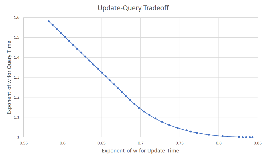
To allow for a faster query time for those problems, we further provide a smooth tradeoff between the update time and the extra query time (see Figure  1). In particular, the other end of this tradeoff curve is an algorithm with $\log^{0.844}n$ update time and $\log^{1+o(1)}n$ extra query time. To the best of our knowledge, in every application, the query algorithm needs to spend at least a constant time on each of the $O(\log n)$ sketches, the query time was already at least $\Omega(\log n)$. This tradeoff point almost does not slow down the query time, while it still improves the update time non-trivially.

To obtain the faster update time, our new algorithms use the following simple observation that connects the worst-case update time to the running time of a computation problem.

As a byproduct, we obtain a “hardness result for proving hardness.” The above proposition implies that proving any super constant update time lower bound, even assuming that the data structure uses optimal space up to a constant factor, would result in a super linear time lower bound for linear space algorithms solving some computation problem in the RAM model, which seems beyond the scope of our current techniques. In particular, Theorem 1 implies that proving any $\log^{\epsilon}n$ lower bound for any problem that admits a $\textrm{lin-skt}(O(1),O(1),\log n)$ solution would imply a non-trivial lower bound for matrix multiplication. We note that although all computational problems admit linear time algorithm in the cell-probe model, Proposition 1 does not imply a streaming algorithm with faster update time in the cell-probe model. We also note that recently, Dvir, Golovnev and Weinstein [DGW19] proved a hardness result for proving space-query time tradeoff lower bounds, but with less “severe” consequences. See more discussions in the next subsection.

The key steps that lead to the improved update time are

• •

  observing that handling a batch of $B$ updates in $o(B\cdot T)$ time implies an $o(T)$ worst-case update time algorithm;

• •

  designing a faster batch update algorithm for linear sketches.

As a running example, let us focus on $\textrm{lin-skt}(2,2,\log n)$, i.e., we partition $[n]$ into two buckets using pairwise hash families, maintain the sum of each bucket, and repeat $T=\log n$ times independently. Note that the straightforward implementation takes $O(\log n)$ space and update time.

Handling $B$ updates in $o(BT)=o(B\log n)$ time naturally implies an algorithm with $o(\log n)$ amortized update time: temporarily store each update in a buffer of size $B$, and handle the updates all at once for every $B$ updates. By applying a trick similar to global rebuilding of Overmars [Ove83], we show that a faster batch update algorithm also leads to lower worst-case update time. To this end, we store two buffers each of size $B$, one of which is the active buffer. We assume that the first buffer is active in the beginning. The new updates are always appended to the active buffer. Then after $B$ updates, the active buffer becomes full. Now we switch the second buffer to be active, and in the next $B$ updates, we fill up the second buffer while gradually flushing the first buffer. That is, if there is an $O(Bt_{u})$ time algorithm handling all $B$ updates, we are going to simulate it for $O(t_{u})$ steps in each of the next $B$ updates. Therefore, when the second buffer becomes full again, we will have already emptied the first buffer, and now we can switch the first buffer back to active and start to flush the second buffer. Each update takes $O(t_{u})$ time in worst case. We present the details in Section 3. Note that this reduction does not work for cell-probe algorithms, because it requires us to simulate the algorithm for a small number of steps in each update. Such simulation is only possible on a RAM for a RAM algorithm, but not possible in the cell-probe model for a cell-probe algorithm.

For $\textrm{lin-skt}(2,2,\log n)$, the space usage is $O(\log n)$ words. Hence, we can afford to set $B=\log n$ without using more space (except for a constant factor). We then show that $\log n$ updates can be applied all together in $o(\log^{2}n)$ time. Each update $(u,\Delta)$ adds the $u$-th column of $A$ multiplied by $\Delta$, to $A\nu$. Thus, $\log n$ updates add the sum of $\log n$ columns multiplied by (possibly different) numbers. To compute this sum, it suffices to multiply a $\log n$ by $\log n$ 0-1 matrix, where each column is a column in $A$, by a $\log n$-dimensional vector with $\log n$-bit entries, where each entry is a $\Delta$.

The task is boiled down to the following: a) given $\log n$ indices $u\in[n]$, compute for each $u$, the $u$-th column in $A$, which reduces to evaluating $\log n$ pairwise independent hash functions for each $u$; b) compute the above matrix-vector product. We show that for a carefully chosen pairwise hash family, both parts can be reduced to $\log n\times\log n\times\log n$ 0-1 matrix multiplications.

Finally, we show that this matrix multiplication can be computed in $\log^{2\omega/3}n$ time on a word RAM with word-size $w=\log n$, and $\log^{\omega/2}n$ time on a word RAM${}^{\text{MM}}$, where $\omega<2.373$ is the current matrix multiplication exponent, using $O(\log n)$ words of space.³³ 3 Note that the input and output sizes are both $O(\log n)$ words. We do this by combining the usual recursive approach to designing fast matrix multiplication algorithms, together with larger-than-usual base cases which can be multiplied in constant time using word operations. In the word RAM model, this involves packing many short vectors into two words so that, when the words are multiplied as integers, the pairwise inner products between those vectors can be read off from the result.

The extra query time of the above algorithm is $O(\log^{2\omega/3}n)=O(\log^{1.582}n)$ time, since we will have to complete the buffer-flushing algorithm, before the actual query algorithm can be launched. To reduce the extra query time, we reduce the buffer size, so that flushing the buffer takes only $\log^{1+o(1)}n$ time. The above arguments still apply, but now, the problem is reduced to rectangular matrix multiplication. The buffer size is reduced sufficiently so that the three dimensions in the matrix multiplication problem are very imbalanced. Finally, we present an algorithm that multiplies $w\times w^{\theta}\times w$ 0-1 matrices in $w^{1+o(1)}$ time for some constant $\theta>0$, which is almost linear in the output size.

In Section 3, we present the connection between computing batch update efficiently and faster worst-case update time. In Section 4, we present how to do the batch update using matrix multiplication. In Section 5, we present the matrix multiplication algorithms for small matrices.

Throughout this paper, we write $\tilde{O}$ to hide ${\mathrm{poly}}\log\log(n)$ multiplicative factors, so $\tilde{O}(T)=T\cdot{\mathrm{poly}}\log\log n$ and $\tilde{O}(1)={\mathrm{poly}}\log\log n$. When $q$ is a power of a prime, we write ${\mathbb{F}}_{q}$ for the finite field of order $q$. For $n\in{\mathbb{N}}$, we write $[n]:=\{1,2,\ldots,n\}$.

We focus in this paper on the word RAM model of computation [FW90]. In the model for word size $w$ (typically we pick $w=\Theta(\log n)$ where $n$ is the input size), the algorithm has random access to words of memory, each of which stores $w$ bits. An algorithm is allowed to perform any “standard” word operations, which only take as input a constant number of words, in constant time. Of course, the efficiency of an algorithm can vary depending on what word operations are considered standard; here we consider two options.

In the following, we prove Lemma 1.

In this subsection, we prove Lemma 2.

In this subsection, we describe how to obtain $\log^{1+o(1)}n$ extra query time. Again, we use Proposition 1. The idea is to set the buffer size $B$ to be smaller, so that $B$ updates can be handled in $\log^{1+o(1)}n$ time. Hence, the worst-case update time is $(\log^{1+o(1)}n)/B$. To this end, let $\theta$ be a positive number such that $w\times w^{\theta}\times w$ matrix multiplication can be computed in $w^{1+o(1)}$ time. By Theorem 4, we can set $\theta>0.156$, according to the current best rectangular matrix multiplication algorithm. We set $B=\log^{\theta}n$.

A similar argument to the proof of Theorem 1 shows that the problem reduces to evaluating $\log n$ $c$-wise hash functions on $\log^{\theta}n$ points, as well as computing a matrix-vector product, where the matrix is a 0-1 matrix of size $(k\log n)\times\log^{\theta}n$, and the vector has dimension $\log^{\theta}n$ and $(\log n)$-bit values. Finally, similar to the proofs of Lemma 1 and Lemma 2, both problems can be reduced to computing $\log n\times\log^{\theta}n\times\log n$ matrix multiplication, which takes $\log^{1+o(1)}n$ by the definition of $\theta$. This gives us an algorithm with update time $O(\log^{0.844}n)$, and extra query time $\log^{1+o(1)}n$, proving Theorem 2. We omit the rest of the details.

In this section, we show how to take advantage of the word RAM model to speed up matrix multiplication when the dimensions of the matrices are polynomials in the word size $w$. We begin by reviewing useful notation related to fast matrix multiplication algorithms.

Let ${\mathbb{F}}$ be any field, $a,b,c$ be any nonnegative real numbers, $n$ be any positive integer, and $X=\{x_{i,j}\}_{i\in[n^{a}],j\in[n^{b}]}$, $Y=\{y_{j,k}\}_{j\in[n^{b}],k\in[n^{c}]}$, and $Z=\{z_{i,k}\}_{i\in[n^{a}],k\in[n^{c}]}$ be three sets of formal variables. The rank of $n^{a}\times n^{b}\times n^{c}$ matrix multiplication over ${\mathbb{F}}$, denoted $R_{\mathbb{F}}(\langle n^{a},n^{b},n^{c}\rangle)$, is the smallest integer $r$ such that there are values $\alpha_{i,j,\ell},\beta_{j,k,\ell},\gamma_{i,k,\ell}\in{\mathbb{F}}$ for all $i\in[n^{a}]$, $j\in[n^{b}]$, $k\in[n^{c}]$ and $\ell\in[r]$ such that

We define $\omega_{\mathbb{F}}(a,b,c):=\liminf_{q\in{\mathbb{N}}}\log_{q}(R_{\mathbb{F}}(\langle q^{a},q^{b},q^{c}\rangle))$. It is known (and we will show below in Theorem 5) that $n^{a}\times n^{b}\times n^{c}$ matrix multiplication over ${\mathbb{F}}$ can be performed in $O(n^{\omega_{\mathbb{F}}(a,b,c)+{\varepsilon}})$ field operations. Although $\omega_{\mathbb{F}}(a,b,c)$ may differ depending on the field ${\mathbb{F}}$, all known constructions achieve the same value for all ${\mathbb{F}}$, so we will typically drop the ${\mathbb{F}}$ and simply write $\omega(a,b,c)$ as in past work. We also write $\omega=\omega(1,1,1)$. We note a couple of simple properties:

References

- [AH74] Alfred V Aho and John E Hopcroft. The design and analysis of computer algorithms. Pearson Education India, 1974.
- [AMS99] Noga Alon, Yossi Matias, and Mario Szegedy. The space complexity of approximating the frequency moments. J. Comput. Syst. Sci., 58(1):137–147, 1999.
- [BCS13] Peter Bürgisser, Michael Clausen, and Mohammad A Shokrollahi. Algebraic complexity theory, volume 315. Springer Science & Business Media, 2013.
- [BMM97] Andrej Brodnik, Peter Bro Miltersen, and J Ian Munro. Trans-dichotomous algorithms without multiplication—some upper and lower bounds. In Workshop on Algorithms and Data Structures, pages 426–439. Springer, 1997.
- [CCF04] Moses Charikar, Kevin C. Chen, and Martin Farach-Colton. Finding frequent items in data streams. Theor. Comput. Sci., 312(1):3–15, 2004.
- [CM05] Graham Cormode and S. Muthukrishnan. An improved data stream summary: the count-min sketch and its applications. J. Algorithms, 55(1):58–75, 2005.
- [DGW19] Zeev Dvir, Alexander Golovnev, and Omri Weinstein. Static data structure lower bounds imply rigidity. In Proceedings of the 51st Annual ACM SIGACT Symposium on Theory of Computing, STOC 2019, Phoenix, AZ, USA, June 23-26, 2019., pages 967–978, 2019.
- [FSH04] Kayvon Fatahalian, Jeremy Sugerman, and Pat Hanrahan. Understanding the efficiency of gpu algorithms for matrix-matrix multiplication. In Proceedings of the ACM SIGGRAPH/EUROGRAPHICS conference on Graphics hardware, pages 133–137. ACM, 2004.
- [Fuj08] Noriyuki Fujimoto. Faster matrix-vector multiplication on geforce 8800gtx. In 2008 IEEE International Symposium on Parallel and Distributed Processing, pages 1–8. IEEE, 2008.
- [FW90] Michael L Fredman and Dan E Willard. Blasting through the information theoretic barrier with fusion trees. In Proceedings of the twenty-second annual ACM symposium on Theory of Computing, pages 1–7. ACM, 1990.
- [GU18] François Le Gall and Florent Urrutia. Improved rectangular matrix multiplication using powers of the coppersmith-winograd tensor. In Proceedings of the Twenty-Ninth Annual ACM-SIAM Symposium on Discrete Algorithms, pages 1029–1046. SIAM, 2018.
- [Ind06] Piotr Indyk. Stable distributions, pseudorandom generators, embeddings, and data stream computation. J. ACM, 53(3):307–323, 2006.
- [JW13] T. S. Jayram and David P. Woodruff. Optimal bounds for johnson-lindenstrauss transforms and streaming problems with subconstant error. ACM Trans. Algorithms, 9(3):26:1–26:17, 2013.
- [KNW10] Daniel M. Kane, Jelani Nelson, and David P. Woodruff. On the exact space complexity of sketching and streaming small norms. In Proceedings of the Twenty-First Annual ACM-SIAM Symposium on Discrete Algorithms, SODA 2010, Austin, Texas, USA, January 17-19, 2010, pages 1161–1178, 2010.
- [LG14] François Le Gall. Powers of tensors and fast matrix multiplication. In Proceedings of the 39th international symposium on symbolic and algebraic computation, pages 296–303. ACM, 2014.
- [Li08] Ping Li. Estimators and tail bounds for dimension reduction in l (0 < 2) using stable random projections. In Proceedings of the Nineteenth Annual ACM-SIAM Symposium on Discrete Algorithms, SODA 2008, San Francisco, California, USA, January 20-22, 2008, pages 10–19, 2008.
- [LKC+10] Victor W Lee, Changkyu Kim, Jatin Chhugani, Michael Deisher, Daehyun Kim, Anthony D Nguyen, Nadathur Satish, Mikhail Smelyanskiy, Srinivas Chennupaty, Per Hammarlund, et al. Debunking the 100x gpu vs. cpu myth: an evaluation of throughput computing on cpu and gpu. ACM SIGARCH computer architecture news, 38(3):451–460, 2010.
- [LNN15] Kasper Green Larsen, Jelani Nelson, and Huy L. Nguyên. Time lower bounds for nonadaptive turnstile streaming algorithms. In Proceedings of the Forty-Seventh Annual ACM on Symposium on Theory of Computing, STOC 2015, Portland, OR, USA, June 14-17, 2015, pages 803–812, 2015.
- [Mni09] Volodymyr Mnih. Cudamat: a cuda-based matrix class for python. Department of Computer Science, University of Toronto, Tech. Rep. UTML TR, 4, 2009.
- [Mut05] S. Muthukrishnan. Data streams: Algorithms and applications. Foundations and Trends in Theoretical Computer Science, 1(2), 2005.
- [Ove83] Mark H. Overmars. The Design of Dynamic Data Structures. Lecture Notes in Economic and Mathematical Systems. Springer-Verlag, 1983.
- [TZ12] Mikkel Thorup and Yin Zhang. Tabulation-based 5-independent hashing with applications to linear probing and second moment estimation. SIAM J. Comput., 41(2):293–331, 2012.
- [Wil12] Virginia Vassilevska Williams. Multiplying matrices faster than coppersmith-winograd. In STOC, volume 12, pages 887–898. Citeseer, 2012.