Gravitational Waves from Phase Transition
in Minimal SUSY Model
Naoyuki Haba and Toshifumi Yamada
Institute of Science and Engineering, Shimane University, Matsue 690-8504, Japan
Abstract
Many extensions of the Standard Model include a new gauge group that is broken spontaneously at a scale much above TeV. If a -breaking phase transition occurs at nucleation temperature of - TeV, it can generate stochastic gravitational waves in - Hz range if , which can be detected by ground-based detectors. Meanwhile, supersymmetry (SUSY) may play a crucial role in the dynamics of such high-scale gauge symmetry breaking, because SUSY breaking scale is expected to be at TeV to solve the hierarchy problem. In this paper, we study the phase transition of gauge symmetry breaking in a SUSY model in the SUSY limit. We consider a particular example, the minimal SUSY model. We derive the finite temperature effective potential of the model in the SUSY limit, study a -breaking phase transition, and estimate gravitational waves generated from it.
1 Introduction
Many extensions of the Standard Model (SM) include a new gauge group that is broken spontaneously, important examples being the minimal model [1, 2, 3], the left-right symmetric model [4, 5] and Pati-Salam model [6]. Usually, there is no theoretical reason to expect that the breaking scale of such gauge group is at TeV scale. If the breaking scale is beyond the reach of new gauge boson searches at colliders, observation of stochastic gravitational waves generated from a -breaking phase transition is the key to testing such models [7]. This is because the nucleation temperature of the phase transition is encoded by the peak position of gravitational wave spectrum, and ground-based detectors such as Advanced LIGO [8], Advanced Virgo [9], KAGRA [10], planned Einstein Telescope [11, 12] and planned Cosmic Explorer [13] cover the region of Hz, which corresponds to nucleation temperature of TeV if the speed of phase transition over the Hubble rate is 1000. Recent work on gravitational waves from the breaking of a new visible gauge group that occurs separately from electroweak symmetry breaking includes [14, 15, 16, 17, 18].
If the breaking of a gauge group occurs at a scale much above TeV, supersymmetry (SUSY) may play a crucial role in its dynamics, since we expect SUSY breaking scale to be at TeV to stabilize the electroweak scale with respect to Planck scale. In this paper, therefore, we study the phase transition of a gauge symmetry breaking in a SUSY model and gravitational waves generated from it. We work in the SUSY limit, namely, we assume that the nucleation temperature is above the SUSY breaking scale so that soft SUSY breaking terms are negligible in the study of phase transition. For concreteness, we focus on the minimal SUSY model 11 1 In a different context, gravitational waves in a SUSY model has been discussed in Ref. [19]. , which is by itself highly motivated because it can explain the origin of the seesaw scale, and if is broken by even charges, -parity is derived and accounts for the stability of dark matter. To simplify our analysis on -breaking phase transition, we assume -symmetry of the model. -symmetry is well-motivated by itself because one can forbid term by -symmetry thereby solving the -problem.
Although we concentrate on the minimal SUSY model, our study is applicable to a wide class of -gauge-extended SUSY models that contain superfields with charge and and a gauge singlet to achieve the breaking. Remarkably, this need not be visible, i.e. the SM fields need not be charged under it, for the study of gravitational waves.
We comment in passing that SUSY models are more predictive than non-SUSY models about high-scale -breaking phase transitions. This is because in non-SUSY models where scalar field breaks an extra , no symmetry forbids the Higgs portal term ( denotes the SM Higgs field),
| (1) |
Suppose develops a large vacuum expectation value (VEV) much above the electroweak scale. To achieve the correct electroweak symmetry breaking, one has two options; one fine-tunes the portal coupling so that the emergent mass term is negligible compared to genuine Higgs mass term ; or one assumes that the genuine Higgs mass term nearly cancels the emergent mass term. In the latter case, the study of the -breaking phase transition involves the SM Higgs field and depends on unknown genuine Higgs mass term , in addition to the -breaking scale. This dependence on the genuine Higgs mass term, or equivalently the Higgs portal coupling, has been studied in Ref. [20]. In SUSY models, the Higgs portal coupling is forbidden at the renormalizable level and hence is justifiably neglected.
This paper is organized as follows.
In Section 2, we explain the minimal SUSY model, and derive the finite temperature effective potential for
-breaking VEVs.
In Section 3, we numerically compute the -symmetric Euclidean action for a high-temperature -breaking phase transition,
calculate quantities that determine gravitational wave spectrum,
and estimate stochastic gravitational waves generated from a -breaking phase transition.
Section 4 summarizes the paper.
2 Finite Temperature Effective Potential in the Minimal SUSY Model
2.1 Minimal SUSY Model
The minimal SUSY model is defined as follows: The gauge group is . The field content is that of the minimal SUSY Standard Model (MSSM) plus three isospin-singlet neutrinos and with the following charge assignments.
| (2) |
As usual, for the MSSM fields, the lepton doublets have , the lepton singlets have , the quark doublets have , the quark singlets have , and the Higgs fields have 0. The most general superpotential reads
| (3) | ||||
| (4) |
Here, mass term is absorbed by a redefinition of and . is the neutrino Dirac Yukawa coupling, and is the coupling that generates Majorana mass for the right-handed neutrinos after breaking. By a phase redefinition, we take to be real positive without loss of generality.
From now on, we assume and . This limit is obtained when the model has -symmetry, under which superfield has and have , and the matter superfields have and the Higgs superfields have . Assuming -symmetry is advantageous for explaining the smallness of in . In the rest of the paper, we neglect and work with the -symmetric superpotential,
| (5) | ||||
| (6) |
As the mechanism for SUSY breaking (at zero temperature) is beyond the scope of this paper, we do not discuss soft SUSY breaking gaugino mass. The tree-level scalar potential involving reads 22 2 By abuse of notation, we denote the scalar component by the same character as the superfield.
| (7) | ||||
| (8) |
2.2 Finite Temperature Effective Potential
To compute the one-loop effective potential at zero and finite temperature, we need the field-dependent mass eigenvalues for bosonic and fermionic components. When SUSY is preserved, bosonic and fermionic components have the same set of mass eigenvalues. However, since SUSY is already broken at finite temperature, we must also consider SUSY-breaking configurations of VEVs, e.g., the case with giving -term SUSY breaking, and the case with giving -term SUSY breaking. So, we study the mass eigenvalues of bosonic and fermionic components separately.
We use Landau gauge for gauge theory.
Before deriving the field-dependent mass eigenvalues, we assume that the VEVs at any temperature satisfy
| (9) |
Then, we take advantage of the symmetry to set both to be real positive, and rewrite these VEVs as
| (10) |
The rest of the section is devoted to the study on the potential for .
The -dependent mass eigenvalues for bosonic components are given as follows: We decompose the scalar components of as , where represent CP-even components and CP-odd components. The -dependent mass matrix for is
and that for is
from which mass eigenvalues are obtained by diagonalization. The -dependent masses for , and the MSSM fields are
| (13) |
with
| (14) | |||
| (15) | |||
| (16) |
Note that the mass of the MSSM fields solely comes from -term SUSY breaking. The -dependent mass term for the gauge boson is
| (17) |
The -dependent mass eigenvalues of fermionic components are given as follows. Let denote the fermionic part of , respectively, and let denote gaugino. The -dependent Majorana mass matrix for fermionic components is given by
The mass eigenvalues are obtained by diagonalizing , and are given by , , , , .
It is easy to verify that when so that SUSY is preserved, non-zero mass eigenvalues of bosonic components obtained from Eqs. (2.2)-(17) coincide with those of fermionic components (with the correct counting of degrees of freedom).
Finally, the finite temperature effective potential [21] for is obtained as
| (19) | ||||
| (20) | ||||
| (21) |
Here, Eq. (19) represents the tree-level potential. Eq. (20) is the one-loop effective potential at zero-temperature, with being the renormalization scale in scheme. Eq. (21) is the temperature-dependent part of the potential, with and . denote the -dependent mass eigenvalues for bosonic components, obtained by diagonalizing Eqs. (2.2),(2.2) and from Eqs. (13)-(17), with no duplication for real scalars, 2 duplications for complex scalars and 3 duplications for gauge boson. denote the -dependent mass eigenvalues for fermionic components, which are , , , , , with 2 duplications for each.
At temperature near or above the critical temperature, daisy diagrams cause breakdown of perturbation theory. This problem is remedied by replacing the tree-level masses of bosonic components in Eqs. (2.2)-(17) with loop corrected ones. We follow Ref. [22] and only include -proportional part of the one-loop correction 33 3 This recipe does not provide a good approximation at low temperature, since the decoupling of particles in the loop is not included [23, 24]. The correct recipe is to solve a self-consistency equation derived from the finite temperature effective potential. Ref. [23] has confirmed the appropriateness of the partial dressing procedure [25]. Unfortunately, this procedure has not yet been extended to a multi-field case, which is our case. , and make the following replacements for the mass of the scalar components of and MSSM fields: 44 4 represent the corrected masses for 1st and 2nd generation quark doublets and up-type singlets, and represent those for 3rd generation. Their difference is a large thermal mass via the top quark Yukawa coupling .
| (22) | ||||
| (23) | ||||
| (24) | ||||
| (25) | ||||
| (26) | ||||
| (27) | ||||
| (28) | ||||
| (29) | ||||
| (30) | ||||
| (31) | ||||
| (32) |
Here, the factor on the second and third terms on the right hand side reflects the fact that in SUSY theories, a bosonic loop correction is always accompanied by a fermionic loop correction with the same coupling constant, and that -part of the fermionic one-loop correction to a boson mass is half the bosonic one-loop correction, and hence their sum is times the bosonic one. The bosonic part (i.e. part without factor ) of the second term comes from one-loop corrections via -term and -term quartic couplings, and that of the third term comes from one-loop corrections via gauge couplings. For the longitudinal component of the gauge boson, we replace its mass, , as
| (33) |
while the mass of the transverse component is unchanged.
2.3 Behavior of the Finite Temperature Effective Potential
We numerically evaluate the finite temperature effective potential Eqs. (19)-(21) (with replacements Eqs. (22)-(32)) for several benchmark parameter sets and study its behavior. The benchmarks we take are
and we fix (only one right-handed neutrino has a large Majorana Yukawa coupling). We take , which does not generate a large logarithm because is the only mass scale in the model. Then, the potential scales with , and depends on and temperature only through dimensionless quantities .
In Figs. 1,2,3,4, we present on plane at the critical temperature , at a high temperature slightly above , and at the nucleation temperature (which we will evaluate in the next section).


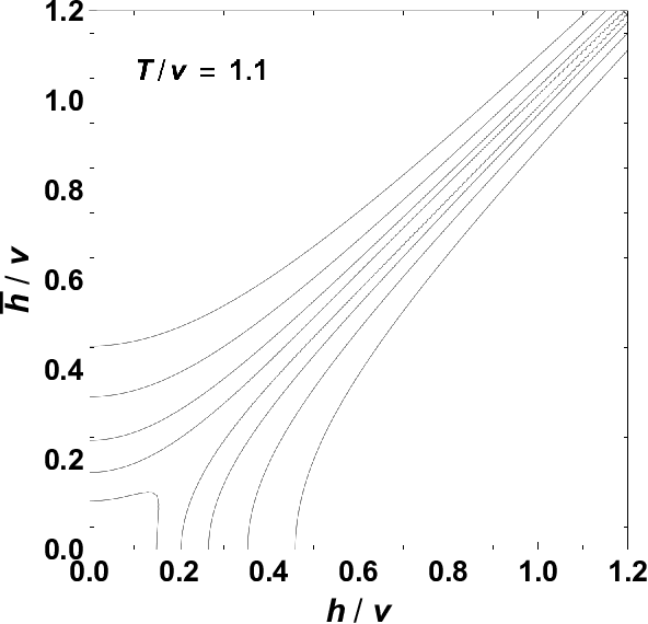


Figs. 1,2,3,4 show that the finite-temperature effective potential is nearly symmetric with respect to and at temperature around or below the critical temperature . This indicates that even though only , not , couples to the right-handed neutrino through Majorana Yukawa coupling , this asymmetry does not affect the potential.
Since the potential is nearly symmetric with respect to and , we can approximate the classical tunneling path from the metastable vacuum to an absolute vacuum by the line , because and hence the equation of motion (with ) for only admits a trivial solution (constant). Under the above approximation, the phase transition is controlled by one-dimensional potential , which allows a qualitative discussion. The one-dimensional potential reads
| (35) | ||||
| (36) | ||||
| (37) |
where are now obtained by diagonalizing
| (38) | ||||
| (39) |
and also from ,
(2 duplications for each),
,
and (2 duplications), while the MSSM particles become irrelevant.
One might guess that increasing and decreasing
enhances the order of phase transition and hence the amount of latent heat,
because the quartic coupling for is mostly , and the field-dependent mass for bosons
(which provides term in high- expansion)
depends on times a big factor 4 or 8.
However, increasing also enhances the thermal mass for these bosons (except for the transverse component of ), which diminishes their impact on the finite temperature effective potential.
Therefore, we expect that the amount of latent heat (which is related to in the next section)
is maximized for and for some moderate value of .
On the other hand, is expected to have a weaker impact on the latent heat
because it only appears in the field-dependent mass for and is not accompanied by a big factor.
All these expectations will be confirmed by the numerical study in the next section.
3 -breaking Phase Transition
3.1 -symmetric Euclidean Action
We calculate the -symmetric Euclidean action [26, 27] for a high-temperature -breaking phase transition from the metastable vacuum to an absolute vacuum where . Although we have seen in Section 2.3 that the potential is nearly symmetric with respect to and , we still consider a multi-field phase transition regarding and as being independent. To compute the -symmetric Euclidean action for a multi-field phase transition, we use CosmoTransitions [28]. From the action computed, we derive the nucleation temperature, , the ratio of the trace anomaly divided by 4 over the radiation energy density of the symmetric phase at the nucleation temperature, , and the speed of the phase transition at the nucleation temperature, . They are defined as follows:
Let denote the Euclidean action. The tunneling rate per volume at temperature is , where is a factor with milder -dependence than . The nucleation temperature satisfies , where denotes the Hubble rate at in the symmetric phase. We estimate as , and further approximate by the -breaking VEV . We estimate as where is the reduced Planck mass and is the effective relativistic degrees of freedom of the SUSY model including fields. (We note that since we will find in all our benchmarks, it is consistent to neglect the impact of soft SUSY breaking due to the -term VEV of in the symmetric phase, on the calculation of the radiation energy density in that phase.) Thus, satisfies the relation
| (40) |
For example, when TeV, the right-hand side of Eq. (40) equals 117, and when TeV, it equals 107. In the following analysis, we fix the right-hand side of Eq. (40) at 117. We comment that we have computed the temperature at which the number of bubbles per Hubble horizon equals one, for the case with the largest supercooling among our benchmarks, by using Eqs. (43),(44), and we have found that this temperature agrees with estimated by Eq. (40) with negligible discrepancy. is given by
| (41) |
satisfies
| (42) |
As with Section 2.3, we take the renormalization scale at , which does not generate a large logarithm because is the only mass scale in the model. We fix the right-hand side of Eq. (40) at 117, thereby neglecting its logarithmic dependence on . With the above choices, a quantity with mass dimension scales with . In particular, scales with , and so we present in the plots.
In Fig. 5, we plot -dependence of the nucleation temperature , for and , with .


We find that has little dependence on , and is much affected by .
In Fig. 6, we plot -dependence of the trace anomaly divided by 4 over the radiation energy density , for and , with .


is significantly enhanced for compared to the case with . Interestingly, is maximized at when , and at when . The dependence on is quite mild compared to those on and .
In Fig. 7, we plot -dependence of the speed of phase transition in units of the Hubble rate at the nucleation temperature in logarithm, for and , with .


is exponentially enhanced for small values of . In contrast, the dependence on is negligible, except for .
Finally, we study how the above quantities vary with . We concentrate on an interesting case where and , which has given the largest in the above plots when . The dependence of on for and is found in Fig. 8.
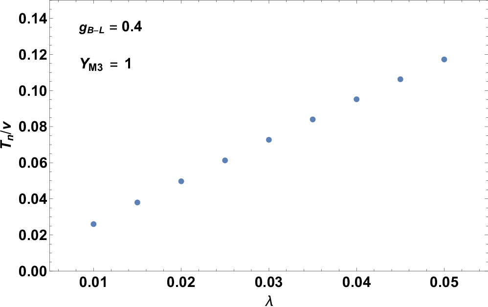
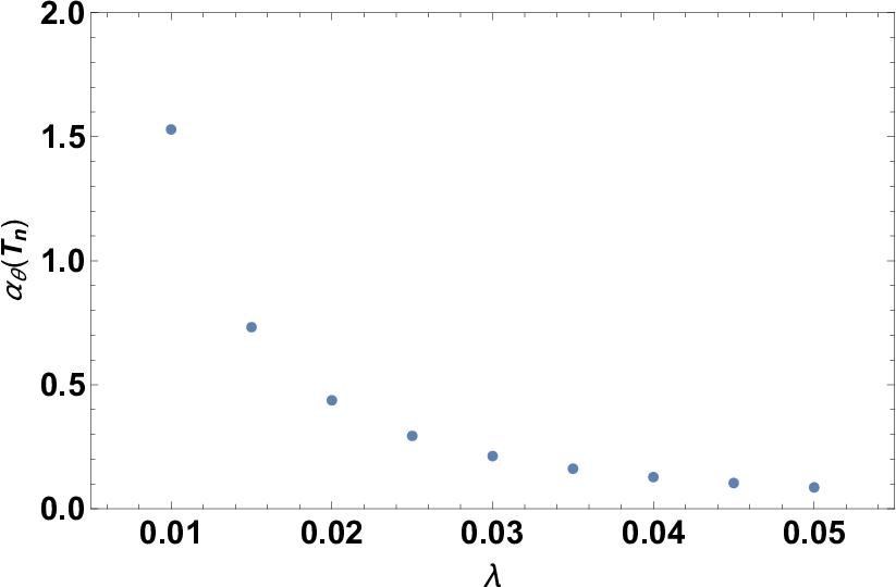
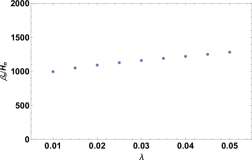
It is observed that increases linearly with ,
and has almost no dependence on ,
while decreases much rapidly with .
3.2 Percolation
When , vacuum energy stored in the meta-stable vacuum causes inflation of meta-stable-vacuum region, which hinders the percolation of absolute-vacuum bubbles [29] (first considered for zero-temperature, quantum phase transitions in [30]). In this subsection, we focus on the benchmark of , which has given , the largest among the benchmarks of Section 3.1, and show that the percolation is completed despite large vacuum energy of the meta-stable vacuum. We can then infer that the percolation is also completed in benchmarks with smaller .
We define the energy such that the vacuum energy of the absolute (broken) vacuum is zero, to be in agreement with the observed almost-zero cosmological constant. Let denote the temperature of the radiation in the meta-stable (symmetric) vacuum. The energy density of the meta-stable vacuum is 55 5 Again, we neglect the impact of soft SUSY breaking due to the -term VEV of , since .
| (43) |
where is the effective relativistic degrees of freedom of the minimal SUSY model, and comes the -term VEV of field.
We have found numerically that the temperature-dependence of the -symmetric Euclidean action in the benchmark of is well approximated by
| (44) |
Here is the temperature at which the potential barrier disappears (then ). Note that is monotonic in this range.
Now we study the probability of finding a point in the meta-stable vacuum, . It is given by [31, 32] 66 6 Unless , the bubble expansion breaks the homogeneity of meta-stable-vacuum region and this region is not described by Friedmann-Robertson-Walker (FRW) metric. Nevertheless, we assume that FRW metric gives a good approximation even for .
| (45) |
where is the fraction of absolute-vacuum bubbles when their overlaps are neglected. is the time corresponding to the critical temperature, denotes the tunneling rate per volume, and denotes the speed of the bubble wall. For later use, we also give the time derivative of ,
| (46) |
Since there is no entropy production in the meta-stable vacuum, we can rewrite and its time derivative in terms of as
| (47) | |||||
| (48) |
where is the Hubble rate of the meta-stable vacuum given from Eq. (43). A criterion for the completion of the percolation is that [29, 33] there is a temperature at which and the physical volume of meta-stable-vacuum region decreases with time, i.e.,
| (49) |
To see if the above criterion is fulfilled in the benchmark of , we compute and from Eqs. (43),(44) with the formula , and plot in units of and in Fig. 9.


From the left panel of Fig. 9, we see that if 10 TeV TeV (which is phenomenologically relevant because it safely satisfies the collider constraint on the gauge boson and it may lead to a gravitational wave spectrum whose peak is covered by Cosmic Explorer and Einstein Telescope) and thus , the relation is fulfilled somewhere in the range , for . Furthermore, the right panel manifests that the relation holds for , and hence holds. Therefore, in the interesting parameter range where 10 TeV TeV, the criterion for the completion of the percolation is fulfilled, namely, the phase transition ends by the coalescence of absolute-vacuum bubbles and the standard cosmology is recovered after that.
We crosscheck the above result using approximate expressions. For a given temperature , let denote a temperature difference for which . Because is a monotonic function with rapid -dependence through the factor , the integrals of Eqs. (43),(44) are dominated by the region around and thus we can make the following approximations:
| (50) | |||||
| (51) |
We find numerically that taking
| (52) |
gives a good order-of-magnitude estimate in the range . By inserting Eqs. (43),(44),(52) into Eq. (50), we see that the relation is satisfied somewhere in the range for 10 TeV TeV and . By taking the ratio of Eqs. (50),(51) and inserting Eqs. (43),(44),(52), we get
| (53) |
which is much greater than in the range ,
and hence the relation is easily satisfied.
3.3 Gravitational Waves
We estimate gravitational waves generated from a -breaking phase transition in the early Universe. In this subsection, we exclusively study the case with , which gives (see the right panel of Fig. 6). This selection is because the study on gravitational wave production in a strong phase transition is currently under development (see, e.g., Refs. [34, 35]), while that in a weaker phase transition is relatively well established.
The sources of gravitational waves from a finite-temperature phase transition are (i) the energy momentum tensor of scalar field in colliding bubbles, (ii) that of sound waves of a surrounding plasma, and (iii) that of magnetohydrodynamic turbulence of a surrounding plasma. On the basis of the claim of Ref. [36] that the bubble wall in plasma always reaches a constant velocity when the next-to-leading order friction is taken into account, and a claim of Ref. [37] that the fraction of energy stored in the bubble wall over the vacuum energy released quickly decreases after the wall reaches the constant velocity, we justifiably neglect source (i). Hence, we only consider sources (ii) and (iii).
For source (ii), it is claimed in Ref. [39] that the energy spectrum of gravitational waves generated by sound waves in a hot plasma in a phase transition with can be expressed as (we rewrite the formula for gravitational wave energy over the critical density we observe today)
| (54) |
where is a typical length scale of fluid motion at the nucleation temperature, is the redshifted value of today, and is a function only of the product . is the enthalpy-weighted root mean square four-velocity of fluid at the nucleation temperature, and is the ratio of enthalpy over energy. In this paper, we adopt Eq. (54). We further identify with the mean bubble separation [41] ( denotes the bubble wall speed), and for , we use a fitting of the simulation results in Ref. [40], which has improved on earlier works [38, 39]. For , we use a fitting formula for the ratio of bulk kinetic energy over vacuum energy derived in Ref. [42], and evaluate it as
| (55) |
The calculation of the bubble wall speed is beyond the scope of the current paper, and we simply assume various values of that appear in the simulations of Ref. [40] and evaluate gravitational wave spectrum in each case.
For source (iii), we estimate its contribution by the following formula in Ref. [43], which is based on Refs. [44, 45]:
| (56) | ||||
| (57) |
where is the red shift factor. We estimate aggressively as following Ref. [43].
The total gravitational wave spectrum is given by
| (58) |
We comment that the relation on which the simulation of Ref. [40] relies, , is not satisfied in our benchmark. This means that sound waves turn into turbulence in less than a Hubble time, which suppresses the sound waves’ contribution to gravitational waves compared to Eq. (54), and may enhance the turbulence’s contribution compared to Eq. (56) [37]. Nevertheless, we use Eqs. (54),(56) in the current analysis.
Our estimate on the total gravitational wave spectrum is presented in Fig. 10, for , TeV, and , and for various values of . The spectrum is given in terms of frequency . The design sensitivity of Advanced LIGO and the sensitivities of Einstein Telescope and Cosmic Explorer for frequency bin of Hz and 2 years of data collection, are estimated from Refs. [46, 12, 13] through the relation dd, where denotes strain power spectral density and denotes the Hubble rate today. These sensitivity curves are overlaid on the plots.


The spectrum around the peak, which is relevant to gravitational wave detection, slides with , with the peak position proportional to and the strength unaltered. This is because is proportional to and are independent of when we fix and fix the right-hand side of Eq. (40). Although the contribution of turbulence Eq. (56) depends on , it is negligible around the peak. Therefore, the spectrum around the peak depends on only through the combination .
Lowering reduces the strength of the spectrum, but does not significantly change its shape and position. This is because decreases for , while and have little or no dependence on when , as seen in the right panels of Figs. 5,6,
We find that in our benchmark with , stochastic gravitational waves are out of reach of the Advanced LIGO design sensitivity for all values of . However, for values of the gauge coupling constant near the weak gauge coupling constant, such as , stochastic gravitational waves can be detected at future Einstein Telescope and Cosmic Explorer. Noting that the spectrum around the peak slides with the -breaking VEV , we see that Einstein Telescope and Cosmic Explorer cover a wide range of the -breaking VEV, which is estimated to be TeV.
We can utilize the position and strength of the peak of the gravitational wave spectrum, to relate
the gauge coupling constant with the -breaking VEV . It proceeds as follows:
For a fixed value of ,
has violent dependence on ,
while it has much milder dependence on the Majorana Yukawa coupling (see Figs. 6,8).
Also, depends only weakly on (see Fig. 8).
Therefore, we can estimate the superpotential coupling from the strength of the gravitational wave spectrum at the peak
through the -dependence of
(see Eq. (54) and note that the spectrum around the peak is dominated by sound waves’ contribution).
Once and are known, we can determine (along with ),
thereby relating the peak position to the -breaking VEV .
The above correspondence between and obtained from the gravitational wave spectrum
offers a clue about the minimal SUSY model, complementing future collider searches for the gauge boson.
4 Summary
We have studied the phase transition of a gauge symmetry breaking in a SUSY model and the production of stochastic gravitational waves associated with it.
We have concentrated on a particular model, which is the minimal SUSY model with -symmetric superpotential.
We have worked in the SUSY limit by assuming that the nucleation temperature is above SUSY breaking scale so that soft SUSY breaking terms are negligible.
We have derived the finite temperature effective potential for the -breaking VEVs ,
and computed the -symmetric Euclidean action of a high-temperature -breaking multi-field phase transition.
We have estimated stochastic gravitational waves generated from the phase transition
in the case with , where and well-established study on gravitational wave production
is available.
We have found that for values of the gauge coupling constant around ,
and for a wide range of the -breaking VEV TeV,
stochastic gravitational waves can be detected at future Einstein Telescope and Cosmic Explorer.
We point out that the position and strength of the peak of the gravitational wave spectrum provides information on the relation between and .
Acknowledgement
This work is partially supported by Scientific Grants by the Ministry of Education, Culture, Sports, Science and Technology of Japan,
Nos. 17K05415, 18H04590 and 19H051061 (NH), and No. 19K147101 (TY).
References
- [1] A. Davidson, “l as the Fourth Color, Quark - Lepton Correspondence, and Natural Masslessness of Neutrinos Within a Generalized Ws Model,” Phys. Rev. D 20, 776 (1979).
- [2] R. E. Marshak and R. N. Mohapatra, “Quark - Lepton Symmetry and B-L as the U(1) Generator of the Electroweak Symmetry Group,” Phys. Lett. 91B, 222 (1980).
- [3] R. N. Mohapatra and R. E. Marshak, “Local B-L Symmetry of Electroweak Interactions, Majorana Neutrinos and Neutron Oscillations,” Phys. Rev. Lett. 44, 1316 (1980) Erratum: [Phys. Rev. Lett. 44, 1643 (1980)].
- [4] R. N. Mohapatra and J. C. Pati, “A Natural Left-Right Symmetry,” Phys. Rev. D 11, 2558 (1975).
- [5] G. Senjanovic and R. N. Mohapatra, “Exact Left-Right Symmetry and Spontaneous Violation of Parity,” Phys. Rev. D 12, 1502 (1975).
- [6] J. C. Pati and A. Salam, “Lepton Number as the Fourth Color,” Phys. Rev. D 10, 275 (1974) Erratum: [Phys. Rev. D 11, 703 (1975)].
- [7] P. S. B. Dev and A. Mazumdar, “Probing the Scale of New Physics by Advanced LIGO/VIRGO,” Phys. Rev. D 93, no. 10, 104001 (2016) [arXiv:1602.04203 [hep-ph]].
- [8] J. Aasi et al. [LIGO Scientific Collaboration], “Advanced LIGO,” Class. Quant. Grav. 32, 074001 (2015) [arXiv:1411.4547 [gr-qc]].
- [9] F. Acernese et al. [VIRGO Collaboration], “Advanced Virgo: a second-generation interferometric gravitational wave detector,” Class. Quant. Grav. 32, no. 2, 024001 (2015) [arXiv:1408.3978 [gr-qc]].
- [10] K. Somiya [KAGRA Collaboration], Class. Quant. Grav. 29, 124007 (2012) doi:10.1088/0264-9381/29/12/124007 [arXiv:1111.7185 [gr-qc]].
- [11] M. Punturo et al., “The Einstein Telescope: A third-generation gravitational wave observatory,” Class. Quant. Grav. 27, 194002 (2010).
- [12] S. Hild et al., “Sensitivity Studies for Third-Generation Gravitational Wave Observatories,” Class. Quant. Grav. 28, 094013 (2011) [arXiv:1012.0908 [gr-qc]].
- [13] B. P. Abbott et al. [LIGO Scientific Collaboration], “Exploring the Sensitivity of Next Generation Gravitational Wave Detectors,” Class. Quant. Grav. 34, no. 4, 044001 (2017) [arXiv:1607.08697 [astro-ph.IM]].
- [14] N. Okada and O. Seto, “Probing the seesaw scale with gravitational waves,” Phys. Rev. D 98, no. 6, 063532 (2018) [arXiv:1807.00336 [hep-ph]].
- [15] V. Brdar, A. J. Helmboldt and J. Kubo, “Gravitational Waves from First-Order Phase Transitions: LIGO as a Window to Unexplored Seesaw Scales,” JCAP 1902, 021 (2019) [arXiv:1810.12306 [hep-ph]].
- [16] D. Croon, T. E. Gonzalo and G. White, “Gravitational Waves from a Pati-Salam Phase Transition,” JHEP 1902, 083 (2019) [arXiv:1812.02747 [hep-ph]].
- [17] T. Hasegawa, N. Okada and O. Seto, “Gravitational waves from the minimal gauged model,” Phys. Rev. D 99, no. 9, 095039 (2019) [arXiv:1904.03020 [hep-ph]].
- [18] V. Brdar, L. Graf, A. J. Helmboldt and X. J. Xu, “Gravitational Waves as a Probe of Left-Right Symmetry Breaking,” JCAP 1912, no. 12, 027 (2019) [arXiv:1909.02018 [hep-ph]].
- [19] W. Buchmüller, V. Domcke, K. Kamada and K. Schmitz, “The Gravitational Wave Spectrum from Cosmological Breaking,” JCAP 1310, 003 (2013) [arXiv:1305.3392 [hep-ph]].
- [20] P. S. B. Dev, F. Ferrer, Y. Zhang and Y. Zhang, “Gravitational Waves from First-Order Phase Transition in a Simple Axion-Like Particle Model,” JCAP 1911, no. 11, 006 (2019) [arXiv:1905.00891 [hep-ph]].
- [21] L. Dolan and R. Jackiw, “Symmetry Behavior at Finite Temperature,” Phys. Rev. D 9, 3320 (1974).
- [22] M. E. Carrington, “The Effective potential at finite temperature in the Standard Model,” Phys. Rev. D 45, 2933 (1992).
- [23] D. Curtin, P. Meade and H. Ramani, “Thermal Resummation and Phase Transitions,” Eur. Phys. J. C 78, no. 9, 787 (2018) [arXiv:1612.00466 [hep-ph]].
- [24] A. Mazumdar and G. White, “Review of cosmic phase transitions: their significance and experimental signatures,” Rept. Prog. Phys. 82, no. 7, 076901 (2019) [arXiv:1811.01948 [hep-ph]].
- [25] C. G. Boyd, D. E. Brahm and S. D. H. Hsu, “Resummation methods at finite temperature: The Tadpole way,” Phys. Rev. D 48, 4963 (1993) [hep-ph/9304254].
- [26] A. D. Linde, “Fate of the False Vacuum at Finite Temperature: Theory and Applications,” Phys. Lett. 100B, 37 (1981).
- [27] A. D. Linde, “Decay of the False Vacuum at Finite Temperature,” Nucl. Phys. B 216, 421 (1983) Erratum: [Nucl. Phys. B 223, 544 (1983)].
- [28] C. L. Wainwright, “CosmoTransitions: Computing Cosmological Phase Transition Temperatures and Bubble Profiles with Multiple Fields,” Comput. Phys. Commun. 183, 2006 (2012) [arXiv:1109.4189 [hep-ph]].
- [29] J. Ellis, M. Lewicki and J. M. No, “On the Maximal Strength of a First-Order Electroweak Phase Transition and its Gravitational Wave Signal,” JCAP 1904, 003 (2019) [arXiv:1809.08242 [hep-ph]].
- [30] A. H. Guth and E. J. Weinberg, “Could the Universe Have Recovered from a Slow First Order Phase Transition?,” Nucl. Phys. B 212, 321 (1983).
- [31] A. H. Guth and S. H. H. Tye, “Phase Transitions and Magnetic Monopole Production in the Very Early Universe,” Phys. Rev. Lett. 44, 631 (1980) Erratum: [Phys. Rev. Lett. 44, 963 (1980)].
- [32] A. H. Guth and E. J. Weinberg, “Cosmological Consequences of a First Order Phase Transition in the SU(5) Grand Unified Model,” Phys. Rev. D 23, 876 (1981).
- [33] M. S. Turner, E. J. Weinberg and L. M. Widrow, “Bubble nucleation in first order inflation and other cosmological phase transitions,” Phys. Rev. D 46, 2384 (1992).
- [34] D. Cutting, M. Hindmarsh and D. J. Weir, “Vorticity, kinetic energy, and suppressed gravitational wave production in strong first order phase transitions,” arXiv:1906.00480 [hep-ph].
- [35] A. R. Pol, S. Mandal, A. Brandenburg, T. Kahniashvili and A. Kosowsky, “Numerical Simulations of Gravitational Waves from Early-Universe Turbulence,” arXiv:1903.08585 [astro-ph.CO].
- [36] D. Bodeker and G. D. Moore, “Electroweak Bubble Wall Speed Limit,” JCAP 1705, 025 (2017) [arXiv:1703.08215 [hep-ph]].
- [37] J. Ellis, M. Lewicki, J. M. No and V. Vaskonen, “Gravitational wave energy budget in strongly supercooled phase transitions,” JCAP 1906, 024 (2019) [arXiv:1903.09642 [hep-ph]].
- [38] M. Hindmarsh, S. J. Huber, K. Rummukainen and D. J. Weir, “Gravitational waves from the sound of a first order phase transition,” Phys. Rev. Lett. 112, 041301 (2014) [arXiv:1304.2433 [hep-ph]].
- [39] M. Hindmarsh, S. J. Huber, K. Rummukainen and D. J. Weir, “Numerical simulations of acoustically generated gravitational waves at a first order phase transition,” Phys. Rev. D 92, no. 12, 123009 (2015) [arXiv:1504.03291 [astro-ph.CO]].
- [40] M. Hindmarsh, S. J. Huber, K. Rummukainen and D. J. Weir, “Shape of the acoustic gravitational wave power spectrum from a first order phase transition,” Phys. Rev. D 96, no. 10, 103520 (2017) [arXiv:1704.05871 [astro-ph.CO]].
- [41] K. Enqvist, J. Ignatius, K. Kajantie and K. Rummukainen, “Nucleation and bubble growth in a first order cosmological electroweak phase transition,” Phys. Rev. D 45, 3415 (1992).
- [42] J. R. Espinosa, T. Konstandin, J. M. No and G. Servant, “Energy Budget of Cosmological First-order Phase Transitions,” JCAP 1006, 028 (2010) [arXiv:1004.4187 [hep-ph]].
- [43] C. Caprini et al., “Science with the space-based interferometer eLISA. II: Gravitational waves from cosmological phase transitions,” JCAP 1604, 001 (2016) [arXiv:1512.06239 [astro-ph.CO]].
- [44] C. Caprini, R. Durrer and G. Servant, “The stochastic gravitational wave background from turbulence and magnetic fields generated by a first-order phase transition,” JCAP 0912, 024 (2009) [arXiv:0909.0622 [astro-ph.CO]].
- [45] P. Binetruy, A. Bohe, C. Caprini and J. F. Dufaux, “Cosmological Backgrounds of Gravitational Waves and eLISA/NGO: Phase Transitions, Cosmic Strings and Other Sources,” JCAP 1206, 027 (2012) [arXiv:1201.0983 [gr-qc]].
- [46] B. P. Abbott et al., “Sensitivity of the Advanced LIGO detectors at the beginning of gravitational wave astronomy,” Phys. Rev. D 93, no. 11, 112004 (2016) Addendum: [Phys. Rev. D 97, no. 5, 059901 (2018)] [arXiv:1604.00439 [astro-ph.IM]].