Modeling and Performance Analysis in Cache-enabled Millimeter Wave HetNets with Access and Backhaul Integration

In this paper, with the aid of stochastic geometry approach, a tractable analytical network model is proposed for characterizing the performance of our mABHetNets. As it is shown in Fig. 1, downlink communication in a two-tier mABHetNets is considered. The first tier of mABHetNets consist of lower-power SBSs while the second tier consists of higher-power MBSs. The MBSs is connected to the mobile core network by high-capacity optical fiber links. Besides, the MBSs provide wireless backhaul connections to the SBSs via broad mmWave spectrum. The locations of the MBSs and SBSs are assumed to follow independent Poisson point processes (PPPs), which are denoted by $\Phi_{m}\in\mathbb{R}_{2}$ and $\Phi_{s}\in\mathbb{R}_{2}$ with densities and $\lambda_{m}$ and $\lambda_{s}$, respectively. Both MBSs and SBSs provide the access service to the users, which is also modeled according to independent homogeneous PPPs $\Phi\in\mathbb{R}_{2}$ with density $\lambda$. $\lambda$ is assumed to be sufficiently larger than $\lambda_{m}$ and $\lambda_{s}$ so that each BS has at least one associated UE in its coverage area. The access link is also using mmWave spectrum. The above model where the nodes are distributed using PPPs has been shown to be quite effective for system-level performance evaluation of cellular networks [20].

The file library is denoted by $\mathcal{F}$ and there are $|\mathcal{F}|=F$ files in the library. It is assumed that each file has the equal size [21] for mathematical tractability and notational simplicity. Note that when the file sizes are different from each other, such assumption can still hold since those files can be divided into chunks of equal size. Different files have different popularities. The file popularity distribution changes with time slowly so that it can be regarded as static [22]. Then, based on collected statistical information and the machine learning algorithm, the file popularity can often be predicted [23]. Zipf distribution is widely used to model the popularity of file $f$, $\forall f\in\{1,...,F\}$: the probability of the $f$-th file is $p_{f}=\frac{f^{-\gamma_{p}}}{\sum_{g=1}^{F}g^{-\gamma_{p}}},$ where $\gamma_{p}$ is the Zipf exponent reflecting different levels of skewness of the distribution[24, 25]. The typical value of $\gamma_{p}$ is between 0.5 and 1.0, where higher value causes more “peakiness” of the distribution [25].

For the cache-enabled MBS and SBS, the cache capacity of the SBS and MBS are denoted by $F$ and $C$ (file units), respectively. As each MBS is often equipped with large cache capacity, we assume that the MBS can cache the total file library [26]. In this paper, the most popular caching strategy is applied for each BS : each BS caches the most popular contents until its storage is full[17]. Hence, the cache hit ratio of a SBS can be calculated as

The mmWave based wireless link can be either line of sight (LOS) or non-line of sight (NLoS) transmission. Then, we consider the following path loss function defined in [27]:

together with the LoS probability $\mathcal{P}_{\mathrm{L}}(r)=\min\left(\frac{18}{r},1\right)(1-e^{-\beta r})+e^{-\beta r}$ and $r$ is the transmission distance. $\beta\geq 0$ is the parameter that captures density and size of obstacles between the transmitter and the reveicer. As $\beta$ increases, the size and density of obstacles increase, which results in lower probability of LoS transmission. The propagation is always in LOS condition when $r\leq 18m$. In practice, this implies that, for denser mABHetNets, the probability of LOS coverage is very close to one and some NLOS transmission could be neglected.

By involving the cache power consumption, we give the power model of one MBS and one SBS as follows[18]:$\rho_{m}P_{m}^{tr}+P_{m}^{fc}+P_{m}^{ca}=\rho_{m}P_{m}^{\mathrm{tr}}+P_{m}^{\mathrm{fc}}+w_{\mathrm{ca}}F,\rho_{s}P_{s}^{tr}+P_{s}^{fc}+P_{s}^{ca}=\rho_{s}P_{s}^{tr}+P_{\mathrm{s}}^{\mathrm{fc}}+w_{\mathrm{ca}}C$ where $P_{m}^{tr}$ and $P_{s}^{tr}$ denote transmit powers consumed at a MBS and a SBS, respectively. $\rho_{m}(\rho_{s})$ reflects the impact of power amplifier and cooling on transmit power. $P_{m}^{fc}(P_{s}^{\mathrm{fc}})$ is the fixed circuits-related power consumption at a BS. $P_{m}^{ca}(P_{s}^{ca})$ is the power consumption for caching files at a BS. Usually, $P_{m}^{fc}(P_{s}^{fc})$ is assumed to be a fixed power consumption constant[28]. To quantify power consumption for caching, we adopt a power-proportional model, which is widely used in cache enabled radio access network [18, 19]. In the power-proportional model, the caching power consumption is proportional to the cache capacity. Then, the caching power consumption of the MBS and SBS are given as follows: $P_{m}^{ca}=w_{ca}F,~P_{s}^{ca}=w_{ca}C$, where $\omega_{ca}$ is the power coefficient of cache hardware in watt/bit. $F$ is the total size of all the files. Here, we assume that the cache storage of the MBS is large enough and the library of all files are cached in MBS [26]. $C$ is the cache storage of a SBS in file unit.

For each SBS, since the total power consumption $P_{s}^{tot}$ is usually given, we can get $P_{s}^{tr}=\frac{P_{s}^{tot}-P_{\mathrm{s}}^{\mathrm{fc}}-w_{\mathrm{ca}}C}{\rho_{s}}$ $=P^{\prime}_{s}-{w^{\prime}}_{\mathrm{ca}}^{s}C$, where $P^{\prime}_{s}=\frac{P_{s}^{tot}-P_{\mathrm{s}}^{\mathrm{fc}}}{\rho_{s}}$ and ${w^{\prime}}_{ca}^{s}=\frac{w_{ca}}{\rho_{s}}$. Here, we assume that the MBS has a large cache capacity and contains all the files in the file library. The total power consumption of a MBS is $P_{m}^{tot}$. Then the $P_{m}^{tr}=\frac{P_{m}^{tot}-P_{\mathrm{m}}^{\mathrm{fc}}-w_{\mathrm{ca}}C}{\rho_{m}}=P^{\prime}_{m}-{w^{\prime}}_{\mathrm{ca}}^{m}F$ is fixed where $P^{\prime}_{m}=\frac{P_{m}^{tot}-P_{\mathrm{m}}^{\mathrm{fc}}}{\rho_{m}}$ and ${w^{\prime}}_{ca}^{m}=\frac{w_{ca}}{\rho_{m}}$. Note that considering the total power consumption, the maximum cache capacity is $\frac{P_{s}^{tot}}{w_{\mathrm{ca}}}$.

The analysis in this paper is done for the user located at the origin referred to as the typical user. Therefore, the signal-to-interference-plus-noise ratio (SINR) of a typical user at a random distance $r$ from its associated SBS and MBS are

where $B_{s},B_{m}$ are the association bias factor of SBS and MBS. $h_{s},h_{m}$ are the small-scale fadings from SBS and MBS. $L(r_{m}),L(r_{s})$ are the path losses from the serving SBS or MBS to the typical user. $r_{s}$ ($r_{m}$) is the distance between the assocation SBS $b_{s,0}$ (assocation MBS $b_{m,0}$) and the typical user. $r_{s,i}$($r_{m,l}$) is the distance between the $i$-th SBS($l$-th MBS )and the typical user. $N_{0}$ is the additive white Gaussian noise component.

To backhaul the data traffic of the SBSs, the MBS provides the wireless backhaul link. For a typical SBS that a random distance $r_{bh}$ from its associated MBS, the SINR of the signal from the MBS to the SBS in downlink backhaul is then given as,

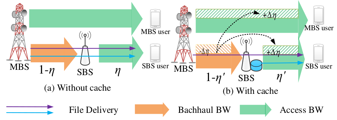
In this paper, we focus on the downlink data transmission using the mmWave spectrum. In Fig.2, both the access link and backhaul link use the mmWave spectrum. To avoid the interference between the access and backhaul link, the access and backhaul use orthogonal spectrum resources. The total mmWave bandwidth $W$ for downlink transmission is partitioned into two parts: $W_{ac}=\eta W$ for access and $W_{bh}=(1-\eta)W$ for backhaul. $\eta\in[0,1]$ is access-backhaul bandwidth partition ratio and denotes the part of spectrum for access link. The file delivery is both related with the access link and backhaul link. Then by changing the partition ratio, both the access rate and backhaul rate in the same transmission path can maintain an effective transmission. When the cache is introduced, cached files can directly delivered from SBS and the backhaul traffic can be saved. Thus, part mmWave spectrum resource in backhaul link can be shifted to access link and the data rate is improved.

First of all, we need to derive the probability distribution function (PDF) of the distance between the typical user and its nearest BS. We focus on the typical user at the origin. When the typical user communicates with the closest BS at a distance $r$, no other BS can be closer than $r$. In other words, all interfering BSs must be farther than $r$. Since the typical user is associated with the closest BS via either LoS or NLoS channel, we derive these PDFs in following Lemma, respectively

In mABHetNets, due to the different transmission path (i.e., LoS and NLoS) and the densities of the SBS and MBS, we need to analyze the probability that a user is associated with SBS tier or with MBS tier. Besides, since in the SBS backhaul association, SBS may be associated with MBS via different transmission paths, different SBS backhaul association probabilities should be derived.

To study the APT and ASE performance of mABHetNets, we need first investigate the SINR distribution of the user covered by SBS/MBS tier via access link or the SINR distribution of the SBS covered by MBS via backhaul link. This SINR distribution is defined as the SINR coverage probability that the received SINR is above a pre-designated threshold $\gamma$:

Since the user is covered either by SBS tier or by MBS tier, we first give the two SINR distributions. Then we give the SINR distribution of the typical SBS when it is covered by MBS.

APT captures the average number of bits that can be received by the user per unit area per unit bandwidth given a pre-designated threshold $\gamma$ [5]. The definition of APT is

where $\lambda_{k}(k=s,m)$ is the density of SBS or MBS and $W_{k}$ is allocated bandwidth to the user. $\gamma$ is the user’s SINR requirement.

In cache-enable mABHetNets, APT is determined by cache capacity, bandwidth partition and SINR threshold. Then we let APT of cache-enable mABHetNets denoted by

where $\mathcal{R}_{s}$ and $\mathcal{R}_{m}$ are APT of the SBS tier and MBS tier. $C$ is the cache capacity of SBS. $\eta$ is the bandwidth partition between the access link and the backahul link. $\gamma_{0}$ is the SINR threshold to guarantee the user throughout requirement. The following corollaries will give the detailed APT expression.

Before giving the ASE of mABHetNets, the user spectral efficiency should be first analyzed. For a user associated with a SBS, the transmission rate of the user is not only related with the access rate from SBS, but also with the backhaul rate from MBS. When the files are cached at the SBS, then the files can be delivered to user directly. At this time, the wireless backhaul between the SBS and the MBS will not be used. Otherwise, the uncache files will be delivered first through the wireless backhaul link then the access link. Let $\rho$ be the required user spectral efficiency and the $p_{h}$ in (1) be the file hit ratio at the SBS. Then the required wireless backhaul link spectral efficiency is $(1-p_{h})\rho$. The definition of the user spectral efficiency distribution is $\mathbb{P}\left[R>\rho\right]$. Then in the following the proposition, we give the detailed user spectral efficiency distribution of the user.

According to the definition of the ASE in [5], ASE can be expressed as follows:

where $\eta$ is the part of the spectrum allocated to the access link and $C$ is the cache capacity of the SBS. $\mathcal{A}_{s}(\eta,C)$ is the ASE of SBS tier and $\mathbb{P}\left[R_{s}>\rho\right]$ is user’s spectral efficiency distribution when the user is associated with the SBS tier. $\mathcal{A}_{m}(\eta)$ is the ASE of MBS tier and $\mathbb{P}\left[R_{m}>\rho\right]$ is the rate distribution when the user is associated with the MBS tier.

Next, we will derive the $\mathcal{A}_{s}(\eta,C)$ and $\mathcal{A}_{m}(\eta)$, respectively.

Based on the research in [30, 31, 32, 33], under the lower SBS density, mABHetNets will be noise-limited. In mmWave communication systems, mmWave has a high signal transmission strength in LoS links. However, when the density of SBS is lower, the number of LoS link will decrease. The LoS based interferences of the intra-tier and cross-tier can be omitted. Therefore, the noise has a more important influence on the mmWave signal transmission. According to such situation, we want to investigate the ASE in cache-enabled mABHetNets in this noise-limited case.[33].

Here, the density $\lambda_{m}$ of MBS in a real mABHetNets is low and fixed. Therefore, in this section, the low density is referring in particular to the SBS denstiy$\lambda_{s}$.

References

- [1] C. Dehos, J. L. Gonzlez, A. De Domenico, D. Ktnas, and L. Dussopt,“Millimeter-wave Access and Backhauling: The Solution to the Exponential Data Traffic Increase in 5G Mobile Communications Systems?” IEEE Commun. Mag., vol. 52, no. 9, pp. 88–95, Sep. 2014.
- [2] R. Taori and A. Sridharan, “Point-to-Multipoint in-band Mmwave Backhaul for 5G Networks,” IEEE Commun. Mag., vol. 53, no. 1, pp. 195-201, Jan. 2015.
- [3] R. J. Weiler et al., “Enabling 5G Backhaul and Access with Millimeter-waves,” in Proc. IEEE EuCNC 2014, Bologna, 2014, pp. 1-5.
- [4] NR; Study on Integrated Access and Backhaul, document 3GPP TR 38.874, 2017.
- [5] A. AlAmmouri, J. G. Andrews and F. Baccelli, “A Unified Asymptotic Analysis of Area Spectral Efficiency in Ultradense Cellular Networks,” IEEE Trans. Inf. Theory, vol. 65, no. 2, pp. 1236-1248, Feb. 2019.
- [6] X. Zhang and J. G. Andrews, “Downlink Cellular Network Analysis With Multi-Slope Path Loss Models,”IEEE Trans. Commun., vol. 63, no. 5, pp. 1881-1894, May 2015.
- [7] I. Atzeni, J. Arnau and M. Kountouris, “Downlink Cellular Network Analysis With LOS/NLOS Propagation and Elevated Base Stations,” IEEE Trans. Wireless Commun., vol. 17, no. 1, pp. 142-156, Jan. 2018.
- [8] M. Ding, D. Lopez-Perez, G. Mao, P. Wang and Z. Lin, “Will the Area Spectral Efficiency Monotonically Grow as Small Cells Go Dense?,” Proc. IEEE GLOBECOM, San Diego, CA, 2015, pp. 1-7.
- [9] X. Wang, E. Turgut and M. C. Gursoy, “Coverage in Downlink Heterogeneous mmWave Cellular Networks With User-Centric Small Cell Deployment,” IEEE Trans. Veh. Technol., vol. 68, no. 4, pp. 3513-3533, April 2019.
- [10] W. Yi, Y. Liu and A. Nallanathan, “Modeling and Analysis of D2D Millimeter-Wave Networks With Poisson Cluster Processes,” IEEE Trans. Commun., vol. 65, no. 12, pp. 5574-5588, Dec. 2017.
- [11] S. Hur, T. Kim, D. J. Love, J. V. Krogmeier, T. A. Thomas and A. Ghosh, “Millimeter Wave Beamforming for Wireless Backhaul and Access in Small Cell Networks,” IEEE Trans. Commun., vol. 61, no. 10, pp. 4391-4403, Oct. 2013.
- [12] Z. Shi, Y. Wang, L. Huang and T. Wang, “Dynamic Resource Allocation in MmWave Unified Access and Backhaul Network,” Proc. PIMRC, Hong Kong, 2015, pp. 2260-2264.
- [13] C. Saha, M. Afshang and H. S. Dhillon, “Bandwidth Partitioning and Downlink Analysis in Millimeter Wave Integrated Access and Backhaul for 5G,” IEEE Trans. Wireless Commun., vol. 17, no. 12, pp. 8195-8210, Dec. 2018.
- [14] D. Liu, B. Chen, C. Yang and A. F. Molisch, “Caching at the Wireless Edge: Design Aspects, Challenges, and Future Directions,” IEEE Commun. Mag., vol. 54, no. 9, pp. 22-28, 2016.
- [15] M. Tao, E. Chen, H. Zhou and W. Yu, “Content-centric Sparse Multicast Beamforming for Cache-enabled Cloud RAN,” IEEE Trans. Wireless Commun., vol. 15, no. 9, pp. 6118-6131, Sept. 2016.
- [16] X. Xu and M. Tao, “Modeling, Analysis, and Optimization of Coded Caching in Small-cell Networks,” IEEE Trans. Commun., vol. 65, no. 8, pp. 3415-3428, Aug. 2017.
- [17] Y. Chiang and W. Liao, “ENCORE: An Energy-aware Multicell Cooperation in Heterogeneous Networks with Content Caching,”Proc. IEEE INFOCOM, San Francisco, CA, 2016, pp. 1-9.
- [18] D. Liu and C. Yang, “Energy Efficiency of Downlink Networks With Caching at Base Stations,” IEEE J. Sel. Areas Commun., vol. 34, no. 4, pp. 907-922, April 2016.
- [19] F. Gabry, V. Bioglio and I. Land, “On Energy-Efficient Edge Caching in Heterogeneous Networks,” IEEE J. Sel. Areas Commun., vol. 34, no. 12, pp. 3288-3298, Dec. 2016.
- [20] H. Elsawy, E. Hossain, and M. Haenggi, “Stochastic geometry for modeling, analysis, and design of multi-tier and cognitive cellular wireless networks: A survey,”IEEE Commun. Surveys Tuts., vol. 15, no. 3, pp. 996–1019, Jun. 2013.
- [21] J. Llorca et al., “Dynamic In-network Caching for Energy Efficient Content Delivery,” in Proc. IEEE INFOCOM, 2013, pp. 245–249.
- [22] K. Shanmugam, N. Golrezaei, A. G. Dimakis, A. F. Molisch and G. Caire, “FemtoCaching: Wireless Content Delivery Through Distributed Caching Helpers,” IEEE Trans. Inf. Theory, vol. 59, no. 12, pp. 8402-8413, Dec. 2013.
- [23] P. Gill, M. Arlitt, Z. Li, and A. Mahanti, “YouTube Traffic Characterization: A View from the Edge,” in Proc. ACM IMC, San Diego, CA, Oct. 2007.
- [24] L. Breslau, P. Cao, L. Fan, G. Phillips, and S. Shenker, “Web Caching and Zipf-like Distributions: Evidence and Implications,” in Proc. IEEE INFOCOM, 1999, pp. 126–134.
- [25] M. Cha, P. Rodriguez, J. Crowcroft, S. Moon, and X. Amatriain, “Atching Television over An IP Network,” in Proc. ACM SIGCOMM IMC, 2008, pp. 126–134.
- [26] G. Quer, I. Pappalardo, B. D. Rao and M. Zorzi,“Proactive Caching Strategies in Heterogeneous Networks With Deviceto-Device Communications,” IEEE Trans. Wireless Commun., vol. 17, no. 8, pp. 5270-5281, Aug. 2018.
- [27] T. Bai, R. Vaze, and R. Heath, “Analysis of blockage effects on urban cellular networks,” IEEE Trans. Wireless Commun., vol. 13, no. 9, pp. 5070–5083, Sep. 2014.
- [28] C. Shuguang, A. J. Goldsmith, and A. Bahai, “Energy-Constrained Modulation Optimization,” IEEE Trans. Wireless Commun., vol. 4, no. 5,pp. 2349–2360, Sep 2005.
- [29] A. K. Gupta, J. G. Andrews and R. W. Heath, “On the Feasibility of Sharing Spectrum Licenses in mmWave Cellular Systems,” IEEE Trans. Commun., vol. 64, no. 9, pp. 3981-3995, Sept. 2016.
- [30] S. Singh, M. N. Kulkarni, A. Ghosh, and J. G. Andrews, “Tractable Model for Rate in Self-backhauled Millimeter Wave Cellular Networks,”IEEE J. Sel. Areas Commun., vol. 33, no. 10, pp. 2196–2211, Oct. 2015.
- [31] J. G. Andrews, T. Bai, M. N. Kulkarni, A. Alkhateeb, A. K. Gupta, and R. W. Heath, Jr., “Modeling and Analyzing Millimeter Wave Cellular ystems,”IEEE Trans. Commun., vol. 65, no. 1, pp. 403–430, Jan. 2017.
- [32] E. Turgut and M. C. Gursoy, “Coverage in Heterogeneous Downlink Millimeter Wave Cellular Networks,” IEEE Trans. Commun., vol. 65, no. 10, pp. 4463-4477, Oct. 2017.
- [33] B. Yang, G. Mao, M. Ding, X. Ge and X. Tao, “Dense Small Cell Networks: From Noise-Limited to Dense Interference-Limited,” IEEE Trans. Wireless Commun., vol. 67, no. 5, pp. 4262-4277, May 2018.
- [34] B. Yang, G. Mao, M. Ding, X. Ge and X. Tao, “Dense Small Cell Networks: From Noise-Limited to Dense Interference-Limited,” IEEE Trans. Veh. Technol., vol. 67, no. 5, pp. 4262-4277, May 2018.
- [35] T. Bai and R. W. Heath, “Coverage and Rate Analysis for Millimeter-Wave Cellular Networks,” IEEE Trans. Wireless Commun., vol. 14, no. 2, pp. 1100-1114, Feb. 2015.
- [36] 3GPP TR 36.942 V12.0.0, “Radio Frequency (RF) System Scenarios (Release 12),” Sep. 2010.
- [37] M. Ding, P. Wang, D. Lpez-Prez, G. Mao and Z. Lin, “Performance Impact of LoS and NLoS Transmissions in Dense Cellular Networks,” IEEE Trans. Wireless Commun., vol. 15, no. 3, pp. 2365-2380, March 2016.
- [38] M. Peng, K. Zhang, J. Jiang, J. Wang and W. Wang, “Energy-Efficient Resource Assignment and Power Allocation in Heterogeneous Cloud Radio Access Networks,”IEEE Trans. Veh. Technol., vol. 64, no. 11, pp. 5275-5287, Nov. 2015.
- [39] C. Liu and K. L. Fong, “Fundamentals of the Downlink Green Coverage and Energy Efficiency in Heterogeneous Networks,” IEEE J. Sel. Areas Commun., vol. 34, no. 12, pp. 3271-3287, Dec. 2016.
- [40] J. G. Andrews, F. Baccelli, and R. K. Ganti, “A Tractable Approach to Coverage and Rate in Cellular Networks,” IEEE Trans. Commun., vol. 59, no. 11, pp. 3122–3134, 2011.