Design and Experimental Performance of Local Entanglement Witness Operators

An entanglement witness that detects the genuine $N$-qubit entanglement is an observable which is guaranteed to have a non-negative expectation value if applied to any separable state, and a negative expectation value for at least one genuine entangled state Terhal 2002. Therefore, a negative expectation value unambiguously signals the presence of $N$-partite genuine entanglement. A witness $\mathcal{W}$ prepared for the ideal expected state $\ket{\psi}$ is an operator

where $\ket{\psi}$ is a non-separable pure state and $\alpha_{\ket{\psi}}$ is the maximal Schmidt coefficient of all bi-partitions of $\ket{\psi}$ Bourennane et al. 2004.

Note that the witness expectation value is directly related to the quantum state fidelity $F=\bra{\psi}\rho\ket{\psi}$ by $\braket{\mathcal{W}}_{\rho}=\alpha_{\ket{\psi}}-F$, and therefore a sufficiently high quantum state fidelity suffices to signal the presence of entanglement. For many states the state fidelity can be either estimated efficiently Flammia and Liu 2011 or be directly determined Bourennane et al. 2004 via a few measurement settings. For stabilizer states $\ket{\mathcal{S}}$, which we focus on here, the projector $\ket{\mathcal{S}}\bra{\mathcal{S}}$ can be decomposed into a sum of the stabilizers that define the state.

A stabilizer state $\ket{\mathcal{S}}$ Gottesman 1997; Nielsen and Chuang 2010 is an $N$-qubit state completely defined by $N$ independent generators $s_{i}$ (the generator set), which mutually commute and act trivially on the state, $\ket{\mathcal{S}}=s_{i}\ket{\mathcal{S}}$. The Pauli operators $s_{i}$ are tensor products of $N$ single-qubit Pauli operators $\left\{I,X,Y,Z\right\}$ multiplied by factors $\pm 1,\pm i$. We denote the usual single-qubit Pauli operators and the identity as $X$, $Y$, $Z$ and $I$.

The set $\mathcal{S}$ containing all generators and their products (including the identity operator $I$) forms the stabilizer group, containing $2^{N}$ elements, called stabilizers (Fig. 2(c)). We say that $S$ spans $\mathcal{S}$ and we will use the notation $\left[S\right]=\mathcal{S}$.

We will use the fact that the choice of the generator set is not unique, because generators contained in it can be recombined and still generate the same stabilizer state, but may require different measurement settings. A recombined generator set $S^{(R)}$ contains products of the generators in $S$, and these products are controlled by a non-singular $N\times N$ binary matrix $R$:

where $s_{j}^{0}=I$ and $s_{j}^{1}=s_{j}$.

For instance, the following recombined generator set spans the same stabilizer as the generator set in Fig. 2(b):

where the $Z$-type generators have been multiplied by the $X$-type generators of the same plaquette, so they have transformed into stabilizers containing only $Y$ Pauli matrices.

Recombinations preserve the stabilizer $\mathcal{S}$, so they also preserve the projector onto the stabilizer state $\ket{\mathcal{S}}$:

Analogously, a generator subset $W_{\varOmega}\subset\mathcal{S}$ of $n<N$ independent and commuting stabilizers of $\mathcal{S}$ can be recombined by $n\times n$ non-singular binary matrices $R_{\varOmega}$. All the recombined generator subsets $W_{\varOmega}^{(R_{\varOmega})}$ span the same subset of $2^{n}$ stabilizers (including the identity $I$):

Then, the projector onto the common $+1$ eigenspace of all the stabilizers in $W_{\varOmega}$ is preserved under recombinations:

for all $R_{\varOmega}$.

For all non-separable multi-qubit stabilizer states $\ket{\mathcal{S}}$ the maximal Schmidt coefficient of all bipartitions is $\alpha_{\ket{\mathcal{S}}}=1/2$, and the fidelity operator is the projector onto the $+1$ eigenvalue of the $N$ stabilizers. Then, the standard genuine witness constructed for the stabilizer state reads

The standard genuine witness is the same if we use any recombined generator set $S^{(R)}$ instead of $S$ because, as pointed out above, recombinations preserve the projector of Eq. (4). For instance, the genuine witness for the seven-qubit color code is preserved if one uses the recombined generator set $S^{(R)}$ in Eq. (3) instead of $S$ in Fig. 2(b). To compute the expectation value of this witness it is necessary to measure $2^{N}-1$ stabilizers, which becomes in general impractical for large $N$. One way to overcome this problem is to construct modified witness operators that includes a smaller number of terms. One option is to consider what we call the the alternative witness Tóth and Gühne 2005b; Tóth and Gühne 2005a in the following,

This requires measuring only the $N$ stabilizers in a generator set $S$. In this case, substituting $S$ by a recombined generator set $S^{(R)}$ changes the alternative witness, which however remains a genuine witness.

If the stabilizer state $\ket{\mathcal{S}}$ has a generator set $S$ composed entirely by $X$-type and $Z$-type stabilizers $s^{X}_{i}$ and $s^{Z}_{j}$ respectively, i.e. each involving single-qubit Pauli operators $X$ and $Z$ only, (for instance Calderbank-Steane-Shor (CSS) codes Calderbank and Shor 1996; Steane 1996), this allows to construct a two-measurements witness,

Note that its evaluation requires only two measurement settings, with all qubits measured in the $X$ and the $Z$ basis.

For the two-measurement witness we have chosen the measurement settings $X_{1}X_{2}\cdots X_{N}$ and $Z_{1}Z_{2}\cdots Z_{N}$ but rotated versions $\sigma_{1}\sigma_{2}\cdots\sigma_{N}$ and $\sigma_{1}^{\prime}\sigma_{2}^{\prime}\cdots\sigma_{N}^{\prime}$ can be used instead as long as $\sigma_{\mu}\neq\sigma_{\mu}^{\prime}$. For instance, in Ref. Alba et al. 2010 the authors construct modified witnesses for bi-colorable graph states, where one measurement setting consists in measuring $X$ on every even qubit and $Z$ on every odd qubit, and vice versa for the second measurement setting. These operators are witnesses because their expectation value is larger than the expectation value of the standard genuine witness for any state Tóth and Gühne 2005b; Tóth and Gühne 2005a,

which guarantees non-negative expectation values for any separable state $\rho$.

The reduction in the number of measurement settings comes at the price that modified witnesses are in general less tolerant to noise. They detect entanglement only in a subset of the states where the standard genuine witness also detects entanglement.

We now review some key concepts of graph states that enable the construction of the local witnesses as proposed in Alba et al. 2010. A graph state $\ket{\mathcal{G}}$ is an $N$-qubit stabilizer state Hein et al. 2006 associated to an underlying undirected graph, like the one depicted in Fig. 3(a), formed by $N$ sites (representing the qubits) and a set $E$ of links or edges $l=\{\mu,\nu\}$ connecting sites $\mu$ and $\nu$. A graph, like the one in Fig. 3(a), can be represented by a $N\times N$ adjacency matrix $\varGamma$ with elements $\varGamma_{\mu\nu}=1\,(0)$ if the sites $\mu,\,\nu$ are (ar not) linked, or, equivalently, by the $N\times{N\choose 2}$ incidence matrix $M_{E}$,

with the index $\mu$ indicating the $\mu$th site and $l$ one of the ${N\choose 2}$ pairs of sites.

A graph state is non-separable if and only if the underlying graph is connected Hein et al. 2006. A graph is connected if it can not be separated into two components without breaking a link. The rank modulo 2 of $M_{E}$ is related to the number $m$ of connected components of the graph: $\mathrm{rank}\left(M_{E}\right)=N-m$ West 2000. In particular, $\mathrm{rank}\left(M_{E}\right)=N-1$, if the graph is connected.

For a graph state $\ket{\mathcal{G}}$, there is one graph state generator $g_{\mu}$ associated to each qubit $\mu$,

where $\mathcal{N}_{\mu}$ is the neighborhood of the site $\mu$.

An equivalent representation of a graph state is

where controlled-phase gates

act on all pair of qubits (sites) connected by a link in the underlying graph.

We need to define analogous concepts within the subsystem $\varOmega$ where we aim to detect entanglement. From a graph state it is possible to extract a reduced graph state $\ket{\mathcal{G}_{\varOmega}}$ for each subsystem $\varOmega$ of $n<N$ qubits. The underlying graph is the reduced graph (Fig. 3(h)) composed by the sites in $\varOmega$ and the subset of links $E_{\varOmega}\subset E$ connecting them. It is represented by the reduced incidence matrix $M_{E_{\varOmega}}$ (Fig. 3(i)) that describes the links in $E_{\varOmega}$. Thus, the reduced graph is connected and hence, $\ket{\mathcal{G}_{\varOmega}}$ is non-separable, if and only if:

The graph state generators $g_{\varOmega,\mu}$ of the reduced graph state $\ket{\mathcal{G}_{\varOmega}}$ can be obtained from the generator subset of $n$ graph state generators corresponding to the qubits in $\varOmega$ (Fig. 3(g)):

From this set one can construct the reduced graph state generators (Fig. 3(j)),

Here, $g_{\mu\nu}\in\left\{I,X,Z\right\}$ is the single-qubit Pauli operator that appears for qubit $\nu$ in the graph state generator $g_{\mu}\in W_{\varOmega}^{\mathcal{G}}$.

These reduced graph state generators form a complete generator set $G_{\varOmega}$ of the reduced graph state $\ket{\mathcal{G}_{\varOmega}}$ (Fig. 3(i)),

Since the controlled-phase gates equal their inverse operation, the unitary that disentangles $\varOmega$ from the rest $\bar{\varOmega}$ of qubits $U_{\mathrm{dis}}^{\mathcal{G}}\ket{\mathcal{G}}=\ket{\mathcal{G}_{\varOmega}}\otimes\ket{\mathcal{G}_{\bar{\varOmega}}}$ is the product of controlled-phase operations that break the links connecting $\varOmega$ with $\bar{\varOmega}$,

where

This unitary applied to the generator subset $W_{\varOmega}^{\mathcal{G}}$ leads to the reduced graph state generators $g_{\varOmega,\mu}$ (Fig. 3(j))

and hence

Following the approach in Alba et al. 2010, the entanglement of an $N$-qubit state $\rho$ is localized in a subsystem $\varOmega$ by means of local measurements on the rest of qubits $\bar{\varOmega}$. The entanglement does not increase under these measurements, so the remaining entanglement in the reduced state $\rho_{\varOmega}$ obtained after the measurement was present in $\rho$. On $\rho_{\varOmega}$ a genuine witness $\mathcal{W}$ is evaluated to detect the remaining entanglement. The key observation is that, instead of executing these measurements, we can instead evaluate a local entanglement witness $\mathcal{W}_{\varOmega}$ on the global state $\rho$ because the expectation values coincide, $\braket{\mathcal{W}}_{\rho_{\varOmega}}=\braket{\mathcal{W}_{\varOmega}}_{\rho}$. Therefore, a negative expectation value of the local witness $\mathcal{W}_{\varOmega}$ detects the presence of entanglement in the reduced state $\rho_{\varOmega}$, and thus the entanglement in the subsystem $\varOmega$ of the global state $\rho$ is detected.

Let us briefly recall the effect of $Z$ measurements on a pure graph state $\ket{\mathcal{G}}$. All $2^{N-n}$ possible outcomes of the measurements of qubits $\nu$ in $\bar{\varOmega}$ can be represented by a binary number $x$ of length $N-n$, with the bit $x_{\nu}=0\,(1)$ for outcome $+1\,(-1)$. The reduced state obtained from $\ket{G}$ after the outcome $x$ on the measurement of $Z$ on every qubit $\nu\in\bar{\varOmega}$ is $\bm{Z}_{x}\ket{\mathcal{G}_{\varOmega}}$ Hein et al. 2006, i.e. the reduced graph state $\ket{\mathcal{G}_{\varOmega}}$ up to outcome-dependent single-qubit $Z$ operations, $Z_{\mu}^{0}=I_{\mu}$ and $Z_{\mu}^{1}=Z_{\mu}$. The effect of the latter is equivalent to the action of the disentangling unitary in Eq. (19) and tracing over the rest of qubits,

If the same process is applied to a mixed $N$-qubit state $\rho$, the reduced state is

One can check that this reduced state is the average over all possible outcomes states $\rho_{\varOmega,x}$ obtained after the same measurement process, multiplied by the outcome-dependent single-qubit operations,

The normalized state corresponding to outcome $x$

is obtained with a probability $p_{x}$.
Once the reduced state $\rho_{\varOmega}^{\mathcal{G}}$ is obtained, a genuine witness of the form Eq. (1)

allows one to detect entanglement in the region. Again, the expectation value of this genuine witness evaluated in $\rho_{\varOmega}^{\mathcal{G}}$ equals the expectation value of the following local witness evaluated in the original state $\rho$,

yielding, using Eq. (22),

As pointed out in section II.1, $\mathcal{W}^{\mathcal{G}_{\varOmega}}$ acts as a witness only if $\ket{\mathcal{G}_{\varOmega}}$ is a non-separable state. Therefore, $W_{\varOmega}^{\mathcal{G}}$ must be chosen such that the genuine witness $\mathcal{W}^{\mathcal{G}_{\varOmega}}$ is prepared for a non-separable graph state $\ket{\mathcal{G}_{\varOmega}}$.

This expectation value is the average of the genuine witness evaluated on all reduced states after the measurement,

Since $p_{x}$ are positive coefficients, if the expectation value of the local witness is negative, at least one $\braket{\mathcal{W}^{\mathcal{G}_{\varOmega}}}_{\bm{Z}_{x}\rho_{\varOmega,x}\bm{Z}_{x}^{\dagger}}$ with $p_{x}\neq 0$ is also negative, indicating that an outcome state $\rho_{\varOmega,x}$ is non-separable (recall that $\bm{Z}_{x}$ preserves entanglement). Thus, the entanglement has been localized in the subsystem $\varOmega$ by the corresponding measurement.

This is due to the connection between local witnesses and localizable entanglement Verstraete et al. 2004; Popp et al. 2005; Sadhukhan et al. 2017. This entanglement measure provides the maximum amount of entanglement $L_{\varOmega}(\rho)$ that can be localized on average in a subsystem $\varOmega$ by means of local measurements on the rest of qubits. Every measurement $\mathcal{M}$ specifies a set of $2^{N-n}$ outcome states $\rho_{\varOmega,x}$ and probabilities $p_{x}$, so for a given $\mathcal{M}$ the average entanglement localized is:

where $E\left(\rho_{\varOmega,x}\right)$ is an entanglement measure.

As we explained, if a local witness has negative expectation value, there is genuine entanglement in one of the outcome states $\rho_{\varOmega,x}$ with $p_{x}\neq 0$ resulting of the particular measurement of $Z$. Hence, the amount $E\left(\rho_{\varOmega,x}\right)\neq 0$ is non-zero and consequently, the localizable entanglement is non-zero $L_{\varOmega}(\rho)\neq 0$. We can conclude that local witnesses detect the localizable entanglement because a negative expectation value of the first implies that the value of the second is non-zero.

Now we want to construct a witness for the stabilizer state $\ket{\mathcal{S}}$, i.e. we want to measure only stabilizers $s_{i}\in\mathcal{S}$ of its stabilizer. We can show that if we find a generator subset $W_{\varOmega}\subset\mathcal{S}$ that is locally equivalent to some generator subset of graph state generators $W_{\varOmega}^{\mathcal{G}}$, the local witness constructed with $W_{\varOmega}$ instead of $W_{\varOmega}^{\mathcal{G}}$ is also a local witness that detects the entanglement of $\varOmega$.

We say that one generator subset $W_{\varOmega}$ of stabilizers is locally equivalent (LE) to a generator subset $W_{\varOmega}^{\mathcal{G}}$ of graph state generators if there is a local unitary $V_{LE}$ and a recombination $R_{\varOmega}$ such that:

Hence, we can construct the following local witness that is decomposed only into stabilizers of the stabilizer state $\ket{\mathcal{S}}$ and we will call standard local witness:

Note that the standard local witness is locally equivalent to the witness for a graph state $V_{LE}\mathcal{W}_{\varOmega}V_{LE}^{\dagger}=\mathcal{W}_{\varOmega}^{\mathcal{G}}$. Then, the expectation value of $\mathcal{W}_{\varOmega}$ evaluated on an state $\rho$ coincides with the expectation value of $\mathcal{W}_{\varOmega}^{\mathcal{G}}$ evaluated on the locally equivalent state $V_{LE}\rho V_{LE}^{\dagger}$,

which has the same entanglement properties. Again, $\mathcal{W}_{\varOmega}^{\mathcal{G}}$ is a witness only if the reduced graph state $\ket{\mathcal{G}_{\varOmega}}$ associated to $W_{\varOmega}^{\mathcal{G}}$ is non-separable.

If the standard local witness has negative expectation value, the entanglement detected can be understood in an analogous way. In this case, the measurements of the qubit $\nu\in\bar{\varOmega}$ outside the subsystem are performed in the basis $V_{LE}^{-1}Z_{\nu}V_{LE}$. The outcome-dependent correction is $V_{LE}^{-1}\bm{Z}_{x}V_{LE}$, which is again a local unitary operation that does not change the entanglement properties of the outcome states. The average of all the outcome states corrected in this way is

Here the disentangling unitary is

Then, a negative expectation value of the local witness implies that at least one outcome state is genuinely entangled, and therefore entanglement has been localized in $\varOmega$.

Now, the problem reduces to finding the generator subset $W_{\varOmega}$ of stabilizers that constructs a valid local witness for the subsystem $\varOmega$. The conditions on $W_{\varOmega}$ are summarized in the next Proposition.

This takes into account that it is possible that a generator subset $W_{\varOmega}$ can not be transformed directly into some $W_{\varOmega}^{\mathcal{G}}$ by a local unitary, but that there is a recombined generator subset $W_{\varOmega}^{(R_{\varOmega})}$ for which such a local unitary exists. For instance, the following generator subsets of stabilizers of the seven-qubit color code differ only in a recombination $R_{\varOmega}$ but the first one can not be transformed directly into graph state generators:

More concretely, the first two elements $s_{R}^{X}s_{R}^{Z}=Y_{1}Y_{2}Y_{3}Y_{4}$ and $s_{R}^{Z}=Z_{1}Z_{2}Z_{3}Z_{4}$ of $W_{\{1,2,3,4\}}$ can not be transformed into two graph state generators with the same local unitary $V_{LE}$. But the local unitary $V_{LE}=H_{1}H_{2}H_{4}$ composed by three Hadamard operators transforms the stabilizers in $W_{\{1,2,3,4\}}^{(R_{\varOmega})}$ into graph state generators:

Note also that the only condition of the local unitary $V_{LE}$ is that it transforms a generator subset $W_{\varOmega}$ of the stabilizer state $\ket{\mathcal{S}}$ into a generator subset $W_{\varOmega}^{\mathcal{G}}$ of a graph state $\ket{\mathcal{G}}$, but it is not forced to transform $\ket{\mathcal{S}}$ into $\ket{\mathcal{G}}$. This fact will become important below where we prove that the direct method indeed finds more witnesses than the graph-based method.

The evaluation of the standard local witness of Eq. (33) requires the measurement of $2^{n}-1$ stabilizers. This number can be reduced further following the same techniques employed for the modified genuine witnesses. Once a valid subset $W_{\varOmega}$ that satisfies Proposition 1 is found, it can be used to construct modified local witnesses that require less measurement settings. For instance, with $n$ measurements we can compute the value of the alternative local witness:

Similar to the two-measurement local witness, if the subset $W_{\varOmega}$ is entirely composed by $X$-type and $Z$-type stabilizers, one can construct a two-measurements local witness:

that can be evaluated with just two measurement settings. If $W_{\varOmega}$ is not of this form, a recombined generator subset $W_{\varOmega}^{(R_{\varOmega})}$ can be used instead. For instance, the generator subset in Eq. (38) is not of this form because the first element contains Pauli operators $Y$, but the generator subset in Eq. (39) has the right form. In this example one can construct the following two-measurements local witness from the generator subset $W_{\{1,2,3,4\}}^{(R_{\varOmega})}$:

Again, here we have chosen the measurement settings $X_{1}X_{2}\cdots X_{N}$ and $Z_{1}Z_{2}\cdots Z_{N}$, but other pairs can be chosen as well.

Like in Eq. (10), the modified local witnesses are valid witnesses as their expectation value is greater or equal than the expectation value of the standard local witness for every state,

Again, the price of reducing the number of measurements is that the modified local witnesses are in general less tolerant to noise than standard local witnesses.

To obtain a benchmark figure of merit for the robustness of a local witness, we consider Tóth and Gühne 2005a the performance of the witnesses with respect to a noisy model state of the form

which is a mixture of the ideal stabilizer state $\ket{\mathcal{S}}$ and the completely mixed state.

The robustness of a witness is then given by the critical probability $p_{c}$, that guarantees that the expectation value of the witness operator evaluated in the state $\rho_{p}$ is negative, and thus entanglement is detected. The critical probabilities of all witnesses discussed summarized in Table 1.

Moreover, one witness $\mathcal{W}$ is said to be finer than other $\mathcal{W}^{\prime}$ if the expectation value of $\mathcal{W}$ is negative on every state where the expectation value of $\mathcal{W}^{\prime}$ is negative. Thus, there is a positive coefficient $\beta>0$ such that $\braket{\mathcal{W}}_{\rho}\leq\beta\braket{\mathcal{W}^{\prime}}_{\rho}$ for any state $\rho$. In that case, one can be sure that $\mathcal{W}$ detects entanglement if $\mathcal{W}^{\prime}$ detects it. If one witness is finer than another, it is also more robust.

There is a hierarchy between the presented witnesses considering this criteria. First, the standard genuine witness is finer than the modified genuine witnesses Tóth and Gühne 2005b; Tóth and Gühne 2005a:

which again shows that reducing the number of measurements by means of modifying the witnesses leads to a decrease of the tolerance to noise. Similarly, and using the same ideas as in Tóth and Gühne 2005b; Tóth and Gühne 2005a, the standard local witness constructed with the generator subset $W_{\varOmega}$ is finer than the modified witnesses constructed from the same generator subset:

Second, standard local witnesses, for every subsystem $\varOmega$, are finer than the standard genuine witness because the expectation value of the projector in Eq. (33) is bigger than the expectation value of the projector in Eq. (7) for any state $\rho$:

Third, two different standard local witnesses $\mathcal{W}_{\varOmega}$ and $\mathcal{W}_{\varOmega^{\prime}}$ such that the generator subsets $W_{\varOmega}$ and $W_{\varOmega^{\prime}}$ satisfy $\left[W_{\varOmega}\right]\subset\left[W_{\varOmega^{\prime}}\right]$ (therefore, the subsystem $\varOmega$ is included inside the second $\varOmega\subset\varOmega^{\prime}$) satisfy that the first one is finer than the second:

For instance, the standard local witness constructed from $W_{\{2,3\}}=\left\{s_{R}^{X},s_{B}^{Z}\right\}$ is finer than the standard local witness constructed from $W_{\{2,3,4\}}=\left\{s_{R}^{X},s_{B}^{Z},s_{G}^{Z}\right\}$.

In the following we provide recipes how to construct the local witnesses starting from the stabilizers of the state of interest.

We now show how can one use the knowledge of a graph state $\ket{\mathcal{G}}$ that is locally equivalent to a stabilizer state of interest $\ket{\mathcal{S}}$, i.e. $U_{LE}\ket{\mathcal{S}}=\ket{\mathcal{G}}$, to construct local witnesses for this state as illustrated in Fig. 4. Some key properties of graph states are depicted in Fig. 3. It is known that for any stabilizer state such a locally equivalent graph state exists Van den Nest et al. 2004. Within the binary picture of the stabilizer formalism, which we summarize in Appendix A, the problem of finding such a graph state reduces to solving a system of binary equations Hein et al. 2006; Lang and Büchler 2012.

Once the graph state generators have been found, the following stabilizer generator subset for state $\ket{\mathcal{S}}$ in a region $\varOmega$ of interest can be obtained by transforming the graph state generators corresponding to qubits within $\varOmega$,

which satisfies property $(A)$ in Proposition 1. The subset $W_{\varOmega}$ also satisfies property $(B)$ if the underlying graph $\varGamma$ of $\ket{\mathcal{G}}$ is connected within the subsystem $\varOmega$, and this is the case if the incidence matrix $M_{E_{\varOmega}}$ of the reduced graph has rank $n-1$.

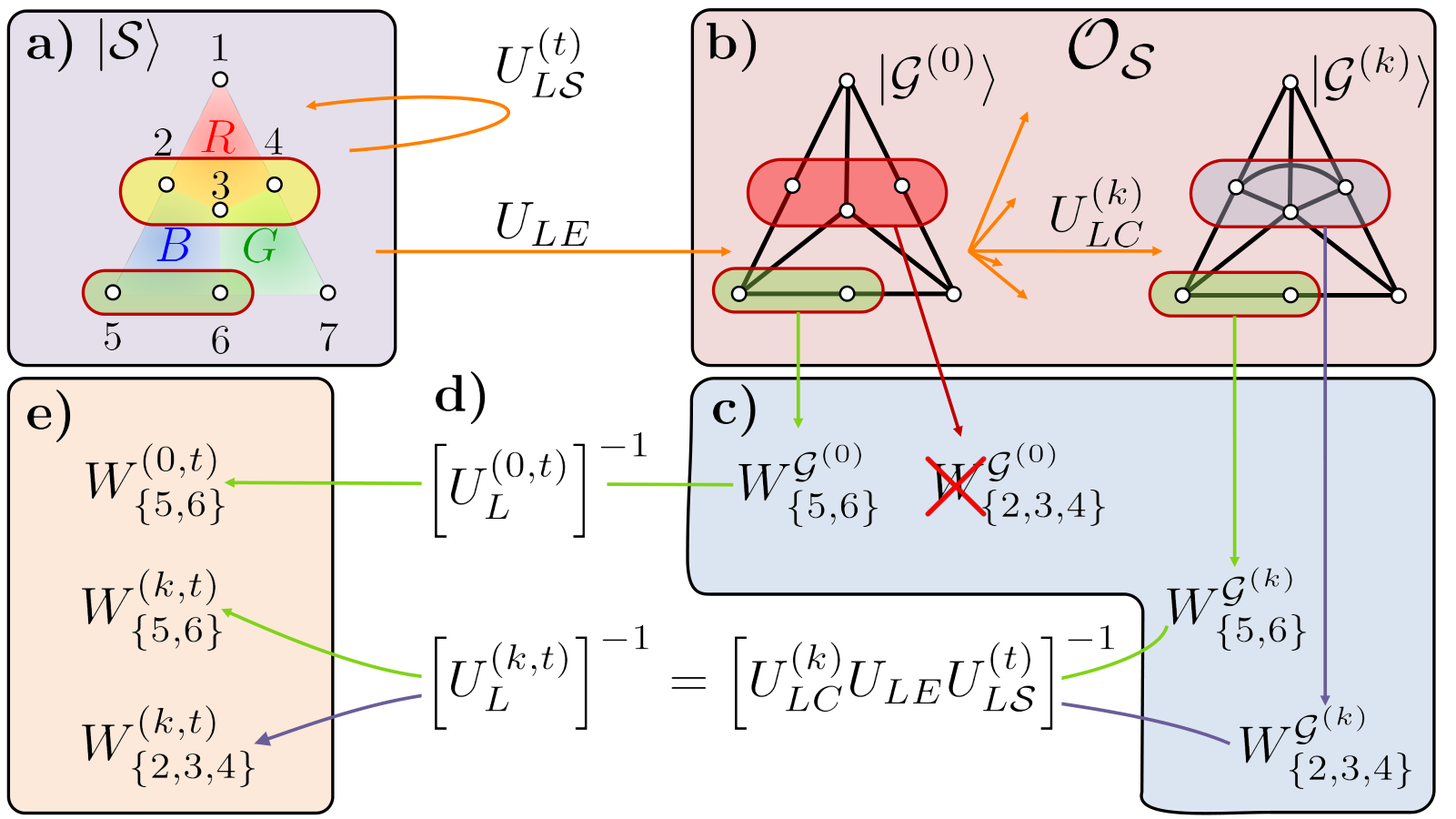
We illustrate this for the example of the first graph state in Fig. 4(b). The local unitary $U_{LE}=H_{1}H_{5}H_{7}$ transforms the seven-qubit stabilizer color code as defined in Fig. 2 into a graph state with the following correspondence between stabilizers and graph state generators:

Whereas any generator subset $W_{\varOmega}$ of these stabilizers satisfies property $(A)$ in Proposition 1, this is not the case for property $(B)$, which depends on the selected subsystem. For instance, since the subsystem $\varOmega=\{5,6\}$ shown in green is connected, the generator subset $W_{\{5,6\}}=\left\{s_{B}^{Z}\,,\,s_{R}^{X}s_{L}^{X}\right\}$ indeed constructs a local witness operator,

for this subsystem. In contrast, the subsystem $\{2,3,4\}$ in red is not connected within this graph, thus the generator subset $W_{\{2,3,4\}}=\left\{s_{G}^{X}s_{L}^{X}\,,\,s_{R}^{X}s_{B}^{X}s_{G}^{X}\,,\,s_{B}^{X}s_{L}^{X}\right\}$ does not provide a local witness. This illustrates that construction of a witness using the graph-based approach requires finding a locally equivalent graph state, for which the qubits corresponding to the region of interest are connected.

If the required connectivity within the region $\varOmega$ is not given for the graph state $\ket{\mathcal{G}}$, one can use this state to generate other locally equivalent graph states by local complementation (LC) operations: the entirety of the locally equivalent graph states $\ket{\mathcal{G}^{(1)}},...,\ket{\mathcal{G}^{(k)}},...$ reached in this way is a finite set and corresponds to the orbit of the graph associated to the initial graph state.

Local complementation on a site $\eta$ in a graph (represented by an adjacency matrix $\varGamma$) acts on all possible links between the sites forming the neighborhood $\mathcal{N}_{\eta}$ of site $\eta$ and substitutes them by their complementary, i.e removes the existing links and adds the non-existing ones,

where the sum is modulo 2. The unitary realizing the graph state transformation corresponding to the LC on the graph is given by a product of single-qubit unitary operations Hein et al. 2006,

See Figures 3 (a), (d), (e) for an example of a unitary performing a LC on a graph state.

Then, for each connected subsystem in the underlying graph of each graph state obtained in this manner one can take the generator subset (Fig. 3(g))

and transform these graph state generators back into a subset of generators of the original stabilizer state of interest,

by the inverse chain of local unitary operations corresponding to the sequence of LC operations. Due to the connectivity of the region $\varOmega$ within the graph they originate from, they satisfy Proposition 1 by construction and thereby provide a valid local witness operator for state $\ket{\mathcal{S}}$ within $\varOmega$.

This approach, involving exploration of the orbit of a graph by LC operations, allows one to find local witnesses for any possible subsystem $\varOmega$ of qubits belonging to the stabilizer state. Using additional symmetries of the stabilizer state allows one to find even more witnesses: Such symmetries are local unitary operations $U_{L\mathcal{S}}^{(t)}$, labeled by an index $t$, which act trivially on the stabilizer state $U_{L\mathcal{S}}^{(t)}\ket{\mathcal{S}}=\ket{\mathcal{S}}$ but are themselves not stabilizer operators. These unitaries can be found by means of solving a binary linear system in the binary picture. For instance, for the seven-qubit color code defined in Fig. 2, one of the symmetries is

which transforms the generator set $S$ of Fig. 2 into the recombined generator set $S^{(R)}$ of Eq. (3). Whereas a symmetry leaves the stabilizer $\mathcal{S}$ invariant, it may transform a generator subset $W_{\varOmega}$ into another one that generally will not lead to the same local witness. For instance, the generator subset $W_{\{1,2,3,4\}}$ in Eq. (38) is transformed into a generator subset

that constructs a different local witness because it spans a different set of stabilizers than $W_{\{1,2,3,4\}}$:

Therefore, for every generator subset $W_{\varOmega}^{(k)}$ found with this method, the generator subset $W_{\varOmega}^{(k,t)}=\left[U_{L\mathcal{S}}^{(t)}\right]^{-1}W_{\varOmega}^{(k)}U_{L\mathcal{S}}^{(t)}$ also constructs a local witness that may be different from the one constructed using $W_{\varOmega}^{(k)}$ for the same subsystem.

Interestingly, there can exist even more local witnesses that are not generated using the graph-based approach, but can be found using an alternative method outlined in the following section.

Here, we introduce an alternative method which provides sufficient and necessary criteria to decide if a given generator subset $W_{\varOmega}\subset\mathcal{S}$ of stabilizers constructs a local witness for a subsystem $\varOmega$, i.e. that whether or not it satisfies Proposition 1. This method is illustrated in Fig. 5 with an example. Importantly, the method does not require obtaining the local unitary $V_{LE}$, nor the recombination $R_{\varOmega}$ of Proposition 1. Furthermore, the direct method is based on a set of intuitive criteria, which for simple cases can be checked by inspection.

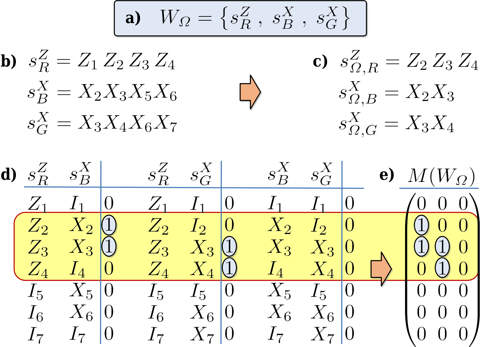
Given a generator subset $W_{\varOmega}\subset\mathcal{S}$ of a stabilizer, we denote with $s_{i\mu}$ the single-qubit Pauli operator of the stabilizer operator $s_{i}\in W_{\varOmega}$ on the qubit $\mu$,

We will need two useful definitions:

The reduced Pauli operators of the generator subset $W_{\varOmega}^{\mathcal{G}}$ of a graph state are the reduced graph state generators $g_{\varOmega,\mu}$ (Fig. 3(j)) defined in Eq. (17).

References

- Gisin et al. (2002) N. Gisin, G. Ribordy, W. Tittel, and H. Zbinden, Rev. Mod. Phys. 74, 145 (2002).
- Cariolaro (2015) G. Cariolaro, Quantum Communications (Springer, Heidelberg, 2015).
- Nielsen (2006) M. A. Nielsen, Rep. Math. Phys. 57, 147 (2006).
- Briegel et al. (2009) H. J. Briegel, D. E. Browne, W. Dur, R. Raussendorf, and M. Van den Nest, Nature , 19 (2009).
- Buhrman et al. (2010) H. Buhrman, R. Cleve, S. Massar, and R. de Wolf, Rev. Mod. Phys. 82, 665 (2010).
- Brunner et al. (2014) N. Brunner, D. Cavalcanti, S. Pironio, V. Scarani, and S. Wehner, Rev. Mod. Phys. 86, 419 (2014).
- Vidal et al. (2003) G. Vidal, J. I. Latorre, E. Rico, and A. Kitaev, Phys. Rev. Lett. 90, 227902 (2003).
- Amico et al. (2008) L. Amico, R. Fazio, A. Osterloh, and V. Vedral, Rev. Mod. Phys. 80, 517 (2008).
- Jurcevic et al. (2017) P. Jurcevic, H. Shen, P. Hauke, C. Maier, T. Brydges, C. Hempel, B. P. Lanyon, M. Heyl, R. Blatt, and C. F. Roos, Phys. Rev. Lett. 119, 080501 (2017).
- Zayed et al. (2017) M. E. Zayed, C. Rüegg, et al., Nat. Phys. 13, 962 (2017).
- Kitaev and Preskill (2006) A. Kitaev and J. Preskill, Phys. Rev. Lett. 96, 110404 (2006).
- Levin and Wen (2006) M. Levin and X.-G. Wen, Phys. Rev. Lett. 96, 110405 (2006).
- Chen et al. (2010) X. Chen, Z.-C. Gu, and X.-G. Wen, Phys. Rev. B 82, 155138 (2010).
- Jahromi and Langari (2017) S. S. Jahromi and A. Langari, J. Phys. A 50, 145305 (2017).
- Chiara and Sanpera (2018) G. D. Chiara and A. Sanpera, Rep. Prog. Phys. 81, 074002 (2018).
- Ryu and Takayanagi (2006) S. Ryu and T. Takayanagi, Phys. Rev. Lett. 96, 181602 (2006).
- Almheiri et al. (2015) A. Almheiri, X. Dong, and D. Harlow, J. High Energy Phys. 4, 163 (2015).
- Pastawski et al. (2015) F. Pastawski, B. Yoshida, D. Harlow, and J. Preskill, J. High Energy Phys. 6, 149 (2015).
- Hubeny (2015) V. E. Hubeny, Classical Quant. Grav. 32, 124010 (2015).
- Brown et al. (2016) K. R. Brown, J. Kim, and C. Monroe, New J. Phys. 2, 16034 (2016).
- Barz (2015) S. Barz, J. Phys. B 48, 083001 (2015).
- Bloch et al. (2008) I. Bloch, J. Dalibard, and W. Zwerger, Rev. Mod. Phys. 80, 885 (2008).
- Clarke and Wilhelm (2008) J. Clarke and F. K. Wilhelm, Nature 453, 1031 (2008).
- Li et al. (2011) C.-F. Li, J.-S. Xu, X.-Y. Xu, K. Li, and G.-C. Guo, Nat. Phys. 7, 752 (2011).
- Åke Larsson (2014) J. Åke Larsson, J. Phys. A-Math. Theor. 47, 424003 (2014).
- Ladd et al. (2010) T. D. Ladd, F. Jelezko, R. Laflamme, Y. Nakamura, C. Monroe, and J. L. O’Brien, Nature 464, 45 (2010).
- Georgescu et al. (2014) I. M. Georgescu, S. Ashhab, and F. Nori, Rev. Mod. Phys. 86, 153 (2014).
- Gross et al. (2010) D. Gross, Y.-K. Liu, S. T. Flammia, S. Becker, and J. Eisert, Phys. Rev. Lett. 105, 150401 (2010).
- Flammia et al. (2012) S. T. Flammia, D. Gross, Y.-K. Liu, and J. Eisert, New J. Phys. 14, 095022 (2012).
- Steffens et al. (2017) A. Steffens, C. A. Riofrío, W. McCutcheon, I. Roth, B. A. Bell, A. McMillan, M. S. Tame, J. G. Rarity, and J. Eisert, Quantum Sci. Technol. 2, 025005 (2017).
- Riofrío et al. (2017) C. A. Riofrío, D. Gross, S. T. Flammia, T. Monz, D. Nigg, R. Blatt, and J. Eisert, Nat. Commun. 8, 15305 (2017).
- Cramer et al. (2010) M. Cramer, M. B. Plenio, S. T. Flammia, R. Somma, D. Gross, S. D. Bartlett, O. Landon-Cardinal, D. Poulin, and Y.-K. Liu, Nat. Commun. 1, 149 (2010).
- Ohliger et al. (2013) M. Ohliger, V. Nesme, and J. Eisert, New J. Phys. 15, 015024 (2013).
- Zhao et al. (2017) Y.-Y. Zhao, Z. Hou, G.-Y. Xiang, Y.-J. Han, C.-F. Li, and G.-C. Guo, Opt. Express 25, 9010 (2017).
- Lanyon et al. (2017) B. P. Lanyon, C. Maier, M. Holzäpfel, T. Baumgratz, C. Hempel, P. Jurcevic, I. Dhand, A. S. Buyskikh, A. J. Daley, M. Cramer, M. B. Plenio, R. Blatt, and C. F. Roos, Nat. Phys. 13, 1158 (2017).
- Terhal (2002) B. M. Terhal, Theor. Comput. Sci. 287, 313 (2002).
- Horodecki et al. (2009) R. Horodecki, P. Horodecki, M. Horodecki, and K. Horodecki, Rev. Mod. Phys. 81, 865 (2009).
- Gühne and Tóth (2009) O. Gühne and G. Tóth, Phys. Rep. 474, 1 (2009).
- Wieczorek et al. (2009) W. Wieczorek, R. Krischek, N. Kiesel, P. Michelberger, G. Tóth, and H. Weinfurter, Phys. Rev. Lett. 103, 020504 (2009).
- Pu et al. (2018) Y. Pu, Y. Wu, N. Jiang, W. Chang, C. Li, S. Zhang, and L. Duan, Sci. Adv. 4, 3931 (2018).
- Horodecki and Lewenstein (2000) P. Horodecki and M. Lewenstein, Phys. Rev. Lett. 85, 2657 (2000).
- Hyllus and Eisert (2006) P. Hyllus and J. Eisert, New J. Phys. 8, 51 (2006).
- Zhang et al. (2013) C. Zhang, S. Yu, Q. Chen, and C. H. Oh, Phys. Rev. Lett. 111, 190501 (2013).
- Tóth (2005) G. Tóth, Phys. Rev. A 71, 010301 (2005).
- Souza and Almeida (2009) A. M. C. Souza and F. A. G. Almeida, Phys. Rev. A 79, 052337 (2009).
- Ribeiro and Macedo (2012) A. N. Ribeiro and C. A. Macedo, Phys. Rev. A 86, 022320 (2012).
- Chakraborty et al. (2013) T. Chakraborty, T. K. Sen, H. Singh, D. Das, S. K. Mandal, and C. Mitra, J. Appl. Phys. 114, 144904 (2013).
- Krenn et al. (2014) M. Krenn, M. Huber, R. Fickler, R. Lapkiewicz, S. Ramelow, and A. Zeilinger, Proc. Natl. Acad. Sci. 111, 6243 (2014).
- Huang et al. (2016) Z. Huang, L. Maccone, A. Karim, C. Macchiavello, R. J. Chapman, and A. Peruzzo, Sci. Rep. 6, 27637 (2016).
- Ding et al. (2016) D.-S. Ding, W. Zhang, S. Shi, Z.-Y. Zhou, Y. Li, B.-S. Shi, and G.-C. Guo, Light. Sci. Appl. 5, 16157 (2016).
- Howland et al. (2016) G. A. Howland, S. H. Knarr, J. Schneeloch, D. J. Lum, and J. C. Howell, Phys. Rev. X 6, 021018 (2016).
- Brandão (2005) F. G. S. L. Brandão, Phys. Rev. A 72, 022310 (2005).
- Eisert et al. (2007) J. Eisert, F. G. S. L. Brandão, and K. M. R. Audenaert, New J. Phys. 9, 46 (2007).
- Gühne et al. (2008) O. Gühne, M. Reimpell, and R. F. Werner, Phys. Rev. A 77, 052317 (2008).
- Cianciaruso et al. (2016) M. Cianciaruso, T. R. Bromley, and G. Adesso, New J. Phys. 2, 16030 (2016).
- Branciard et al. (2013) C. Branciard, D. Rosset, Y.-C. Liang, and N. Gisin, Phys. Rev. Lett. 110, 060405 (2013).
- Xu et al. (2014) P. Xu, X. Yuan, L.-K. Chen, H. Lu, X.-C. Yao, X. Ma, Y.-A. Chen, and J.-W. Pan, Phys. Rev. Lett. 112, 140506 (2014).
- Nawareg et al. (2015) M. Nawareg, S. Muhammad, E. Amselem, and M. Bourennane, Sci. Rep. 5, 8048 (2015).
- Verbanis et al. (2016) E. Verbanis, A. Martin, D. Rosset, C. C. W. Lim, R. T. Thew, and H. Zbinden, Phys. Rev. Lett. 116, 190501 (2016).
- Bourennane et al. (2004) M. Bourennane, M. Eibl, C. Kurtsiefer, S. Gaertner, H. Weinfurter, O. Gühne, P. Hyllus, D. Bruß, M. Lewenstein, and A. Sanpera, Phys. Rev. Lett. 92, 087902 (2004).
- Tóth and Gühne (2005a) G. Tóth and O. Gühne, Phys. Rev. A 72, 022340 (2005a).
- Tóth and Gühne (2005b) G. Tóth and O. Gühne, Phys. Rev. Lett. 94, 060501 (2005b).
- Shahandeh et al. (2017) F. Shahandeh, M. Ringbauer, J. C. Loredo, and T. C. Ralph, Phys. Rev. Lett. 118, 110502 (2017).
- Liang et al. (2015) Y.-C. Liang, D. Rosset, J.-D. Bancal, G. Pütz, T. J. Barnea, and N. Gisin, Phys. Rev. Lett. 114, 190401 (2015).
- Zhao et al. (2016) Q. Zhao, X. Yuan, and X. Ma, Phys. Rev. A 94, 012343 (2016).
- Sperling and Vogel (2013) J. Sperling and W. Vogel, Phys. Rev. Lett. 111, 110503 (2013).
- Sperling and Vogel (2011) J. Sperling and W. Vogel, Phys. Rev. A 83, 042315 (2011).
- Huber and de Vicente (2013) M. Huber and J. I. de Vicente, Phys. Rev. Lett. 110, 030501 (2013).
- Shahandeh et al. (2014) F. Shahandeh, J. Sperling, and W. Vogel, Phys. Rev. Lett. 113, 260502 (2014).
- Alba et al. (2010) E. Alba, G. Tóth, and J. J. Garcia-Ripoll, Phys. Rev. A 82, 062321 (2010).
- Friis et al. (2018) N. Friis, O. Marty, C. Maier, C. Hempel, M. Holzäpfel, P. Jurcevic, M. B. Plenio, M. Huber, C. Roos, R. Blatt, and B. Lanyon, Phys. Rev. X 8, 021012 (2018).
- Amaro et al. (2018) D. Amaro, M. Müller, and A. K. Pal, New J. of Phys. 20, 063017 (2018).
- Verstraete et al. (2004) F. Verstraete, M. Popp, and J. I. Cirac, Phys. Rev. Lett. 92, 027901 (2004).
- Popp et al. (2005) M. Popp, F. Verstraete, M. A. Martín-Delgado, and J. I. Cirac, Phys. Rev. A 71, 042306 (2005).
- Sadhukhan et al. (2017) D. Sadhukhan, S. S. Roy, A. K. Pal, D. Rakshit, A. Sen(De), and U. Sen, Phys. Rev. A 95, 022301 (2017).
- Nielsen and Chuang (2010) M. A. Nielsen and I. L. Chuang, Quantum Computation and Quantum Information (Cambridge University Press, 2010).
- Devitt et al. (2013) S. J. Devitt, W. J. Munro, and K. Nemoto, Rep. Prog. Phys. 76, 076001 (2013).
- Van den Nest et al. (2004) M. Van den Nest, J. Dehaene, and B. De Moor, Phys. Rev. A 69, 022316 (2004).
- Lewenstein et al. (2000) M. Lewenstein, B. Kraus, J. I. Cirac, and P. Horodecki, Phys. Rev. A 62, 052310 (2000).
- Bombin and Martín-Delgado (2006) H. Bombin and M. A. Martín-Delgado, Phys. Rev. Lett. 97, 180501 (2006).
- Nigg et al. (2014) D. Nigg, M. Müller, E. A. Martínez, P. Schindler, M. Hennrich, T. Monz, M. A. Martín-Delgado, and R. Blatt, Science 345, 302 (2014).
- Flammia and Liu (2011) S. T. Flammia and Y.-K. Liu, Phys. Rev. Lett. 106, 230501 (2011).
- Gottesman (1997) D. Gottesman, arXiv:quant-ph/9705052 (1997).
- Calderbank and Shor (1996) A. R. Calderbank and P. W. Shor, Phys. Rev. A 54, 1098 (1996).
- Steane (1996) A. M. Steane, Phys. Rev. Lett. 77, 793 (1996).
- Hein et al. (2006) M. Hein, W. Dür, J. Eisert, R. Raussendorf, M. Van den Nest, and H. J. Briegel, arXiv:quant-ph/0602096 (2006).
- West (2000) D. B. West, Introduction to Graph Theory, 2nd ed. (Prentice Hall, 2000).
- Lang and Büchler (2012) N. Lang and H. P. Büchler, Phys. Rev. A 86, 022336 (2012).
- A. Zeilinger (1992) D. M. G. A. Zeilinger, M. A. Horne, Proceedings of Squeezed States and Quantum Uncertainty, edited by Z. W. Han D., Kim Y.S., Vol. 3135 (NASA Conf. Pub. 3135, 1992) p. 73.
- Dür et al. (2000) W. Dür, G. Vidal, and J. I. Cirac, Phys. Rev. A 62, 062314 (2000).
- Dicke (1954) R. H. Dicke, Phys. Rev. 93, 99 (1954).