Fusion of labeled RFS densities with
minimum information loss
Abstract
This paper addresses fusion of labeled random finite set (LRFS) densities according to the criterion of minimum information loss (MIL). The MIL criterion amounts to minimizing the (weighted) sum of Kullback-Leibler divergences (KLDs) with the fused density appearing as righthand argument of the KLDs. In order to ensure the fused density to be consistent with the local ones when LRFS densities are marginal -generalized labeled multi-Bernoulli (M-GLMB) or labeled multi-Bernoulli (LMB) densities, the MIL rule is further elaborated by imposing the constraint that the fused density be in the same family of local ones. In order to deal with different fields-of-view (FoVs) of the local densities, the global label space is divided into disjoint subspaces which represent the exclusive FoVs and the common FoV of the agents, and each local density is decomposed into the sub-densities defined in the corresponding subspaces. Then fusion is performed subspace-by-subspace to combine local sub-densities into global ones, and the global density is obtained by multiplying the global sub-densities. Further, in order to tackle the label mismatching issue arising in practical applications, a rank assignment optimization (RAO) of a suitably defined cost is carried out so as to match labels from different agents. Moreover, issues concerning implementation of the MIL rule and its application to distributed multitarget tracking (DMT) are discussed. Finally, the performance of the proposed fusion approach is assessed via simulation experiments considering DMT with either the same or different FoVs of the agents.
Index Terms:
Distributed multitarget tracking, Kullback-Leibler divergence, random finite set, data fusion, linear opinion poolI Introduction
Originating from [1], generalized covariance intersection (GCI) has become the most commonly adopted method for the fusion of multi-object densities. As well known, GCI fusion amounts to computing the geometric mean of the local densities [2] and is consistent with the logarithmic opinion pool (LogOP) [3], which aims to aggregate information from multiple probability density functions (PDFs). Relying on the GCI approach, several algorithms have been developed for fusing different types of random finite set (RFS) processes [4, 5, 6, 7, 8, 9]. It has been shown that, based on the principle of minimum discrimination of information (PMDI), the GCI-fused density is the one that minimizes the weighted sum of Kullback-Leibler divergences (KLDs) from the local densities to itself [5, 10] and, from an information-theoretic viewpoint, can be interpreted as the one that leads to minimum information gain (MIG) [11, 12].
Besides GCI fusion, it is possible to exploit the dual fusion rule that leads to minimum information loss (MIL) [11, 13]. Such fusion rule can be obtained also based on the idea of PMDI, where the fused density is defined as the one minimizing the weighted sum of KLDs from itself to the local densities. It has been shown in [14] that the fused density according to MIL turns out to be the weighted arithmetic mean of the local densities, which is consistent with the linear opinion pool (LOP) [3]. However, the MIL rule cannot be directly applied to fuse the majority of RFS densities due to lack of closeness, i.e. the resulting fused RFS density does not in general belong to the same family of the local ones. This prevents, for instance, its direct use in distributed multitarget tracking (DMT) [15] wherein the fused density at a given time serves as prior information for the next recursion. In order to overcome such difficulties, it is proposed to approximate the fused RFS with a multi-object Poisson process (MPP) matching the first-order statistical moment, which results into the so-called arithmetic fusion [16, 17]. It has been shown in [18] that such approximation turns out to be the one that minimizes the average Cauchy-Schwarz divergence (CSD) [19]. However, all the methods of [18, 16, 17] can only be applied to the case where local densities are MPP. In [11], by further exploiting the MIL paradigm, a constraint that the fused density must be within the same family of the local ones is imposed to the PMDI, so that the “best”, in the sense of MIL, density within the considered family is obtained, and such result can be applied to general multi-object processes (i.e., i.i.d. cluster processes).
It has been shown that both GCI and MIL fusion rules are conservative and immune to the problem of double counting of information [2, 20]. Moreover, both of them have their respective advantages and disadvantages. The GCI rule has been proved to guarantee stability in terms of mean-square boundnedess of the estimation error in the context of distributed state estimation (i.e. distributed Kalman filtering) [10, 21, 22]. However, the GCI rule suffers from cardinality inconsistency in the context of multi-object density fusion [23], and is sensitive to misdetections. Conversely, the MIL rule has satisfactory performance in terms of cardinality estimation, while its performance deteriorates with higher false alarm rates [11]. To summarize, in the context of DMT it is more suitable to adopt MIL fusion whenever the detection probability is low, while GCI fusion is preferable whenever dense clutter is present in the area of interest (AoI).
In this paper, the primary concern is in the extension of MIL multi-object fusion to labeled RFS (LRFS) densities. The main advantage of modeling the multi-object state as LRFS is that the trajectory of each object can be obtained directly, while additional track management procedures [24] are needed to extract object trajectories from unlabelled RFS densities. It has been shown in [25] that a general LRFS density can be factored into the product of the joint existence probability (JEP) of the multi-object label set by the corresponding conditional joint PDF (CJPDF). Based on such representation, it is shown in this paper that the fusion of general LRFS densities (defined on the same label space) adopting the MIL rule yields another general LRFS density, and such result can be directly applied to fuse multiple -GLMB densities [26, 27]. However, when the local LRFSs are modeled as M-GLMB [28] or LMB [29] processes, the resulting fused LRFS density is not of the same type of the local ones. Then the idea of [11], where MIL optimization is restricted to the considered specific class of local RFS densities, is exploited; specifically, the “best”, in the MIL sense, fused M-GLMB/LMB of local M-GLMB/LMB densities is found.
In practice, due to the limitation of sensor range, it turns out that the multi-object densities to be fused carry information on different fields-of-view (FoVs), thus implying another challenge of multi-object fusion. In such situation, if the GCI fusion is directly applied, due to its multiplicative nature, the fused density tends to become null outside the common FoV. In this way, the non-common (exclusive) information carried by local densities is lost. Such a problem can be alleviated by taking remedies on the GCI method. Specific remedies are the following.
- -
When multi-object densities are modeled as MPP with Gaussian mixture (GM) representation[30], a uniform initialization of the probability hypothesis density (PHD) for local MPPs can be employed so as to avoid the null-PHD problem [31]. It is also possible to first disengage the Gaussian components (GCs) outside the common FoV with component matching algorithms (e.g. clustering algorithm), and then separately perform fusion on the GCs inside and outside the common FoV with different strategies [32, 33].
- -
When the LMB RFS [29] is employed to model the multi-object state, a promising strategy is to associate to each Bernoulli component (BC) of each local LMB density a specific fusion weight based on the amount of information it carried, and then the fusion weights of BCs which have not been updated by measurements are automatically decreased, thus reducing their effect on the fusion process [34]. Moreover, motivated from the uniform initialization strategy in [31], it is also possible to adopt a density compensation strategy, where the local posterior of each agent undergoes an auxiliary birth process outside its local FoV. As a result, the problem of miss-detections outside the local FoV of each agent can be alleviated [35].
Unlike GCI fusion which essentially performs “intersection” among the agent FoVs, the MIL rule has the potential to correctly fuse multi-object densities defined in different FoVs [18, 11]. However, since each local density has only the information within its own FoV, the JEPs of all label subsets that include targets outside the FoV are always zero. If the MIL rule is directly applied to all the local densities, the JEP of the global density that includes all the targets spread over the whole surveillance area will certainly become null, which means that it is not possible to jointly detect all the existing targets spread over the whole surveillance area.
In this paper, we propose to handle fusion of multi-object densities with different FoVs by applying the MIL rule to mutually disjoint label subspaces, where the label subspaces are obtained by evaluating the exclusive and common FoVs of the agents. The sub-densities, which are defined on different label subspaces, are found by minimizing the KLD from the re-constructed local density (equal to the product of sub-densities) and the corresponding original local density. By combination of the MIL rule and the decomposition strategy, the problem of fusing local LRFS densities defined on different FoVs can be handled. The advantage of the proposed algorithm is that it needs neither aforehand initialization of multi-object densities over the global FoV nor density compensations, so that it can be implemented in a more efficient way.
It should be noted that the proposed MIL fusion rule for multiple LRFS densities is based on the pre-condition that all the involved LRFS densities are defined on the same label space. In practice, however, it is extremely difficult to ensure such assumption due to the fact that the local LRFS densities are propagated independently, thus resulting into the label mismatching (LM) problem [9]. This difficulty can be overcome by setting up associations among labels of different LRFS densities. The existing strategy [9] exploits rank assignment to find the associations, in which each label of the LRFS density with smaller cardinality of the label space will always be associated to a label of another LRFS density. Such strategy works well when all agents have the same FoV, nevertheless, whenever agents have different FoVs, it is also possible that some label of an LRFS density remains unassociated, thus the method in [9] is not suitable. In this paper, we propose to solve the LM problem with different FoVs also by means of the rank assignment problem, where the cost is defined by exploiting an information-theoretic divergence between BCs. In the proposed strategy, the cost that a BC remains unassociated is also defined (which actually represents an upper bound on the divergence between associated BCs in different local LRFS densities), thus the BCs outside the common FoV can be properly found.
To summarize, this paper provides the following main contributions.
- 1)
A novel fusion rule that leads to MIL is proposed to fuse LRFS densities.
- 2)
In combination with a suitable label decomposition strategy, the MIL rule can be directly applied to handle DMT when the agents have different FoVs.
- 3)
A strategy is proposed to solve the LM problem among LRFS densities, thus strengthening the applicability of the proposed algorithms to real scenarios.
Notation
The notation used throughout the paper is summarized hereafter. First, we denote the agent set of a multi-agent system (MAS) as , which consists of agents. Next, all the quantities related to LRFSs will be denoted with boldface symbols. Specifically, we use to denote an LRFS and for the augmented (labelled) single-object state. Further, represents a generic LRFS density, a -GLMB density, an M-GLMB density, and an LMB density. Moreover, a superscript is used to refer to a specific agent, i.e., indicates the local density of agent . Conversely, subscripts of sets will be used to indicate their cardinality. For instance, and denote respectively an LRFS and label set with cardinality . We also define and . For the sake of convenience, in the rest of this paper, the symbols , and their respective full definitions , will be interchangeably used. All the involved spaces will be denoted by blackboard bold symbols. For instance, denotes the state space, and the label space. Further, we use subscripts with space symbols to refer to subspaces, e.g. , where denotes disjoint union (i.e. , for ). Conversely, we use superscripts together with space symbols to refer to the label space of a local LRFS density, i.e. indicates the label space of , for agent . Finally, we define as the set of all subsets of with elements.
II Background
II-A Labeled RFS
In this paper, the multi-object state with cardinality is modeled as an LRFS in which the -th () single-object state is denoted as , denoting the kinematic state space and the label space. From a statistical viewpoint [36], an LRFS is completely characterized by its multi-object density . For a general LRFS density , its joint existence probability (JEP) of label set is given by [25]
| (1) |
Then, it is straightforward to define the conditional joint probability density function (CJPDF) of RFS given label set as [25]
| (2) |
It can be directly seen from the definition (2) that the CJPDF is permutation-invariant, i.e.
| (3) |
where denotes any permutation on numbers , and its -th element ().
For the sake of convenience, we introduce the shorthand notation . Equivalently, any LRFS density can be generally expressed as
| (4) |
Hence, any LRFS density can be completely specified by the JEP and CJPDF according to (4). In particular,
- -
A -GLMB density is specified by [26]
(5) (6) where: is a discrete index set whose elements represent track-to-measurement association hypotheses in the context of multitarget tracking with point measurements; denotes the JEP of under hypothesis which satisfies ; represents the PDF of track conditional on and hypothesis ;
- -
An M-GLMB density , which is defined as -GLMB density marginalized by the discrete index set , is specified by [28]
(7) (8) where denotes the JEP of label set and the PDF of track conditional on label set ;
- -
An LMB density is specified by [29]
(9) (10) where denotes the existence probability (EP) of track with label and the corresponding PDF.
Remark 1.
Besides the above mentioned definition as marginalization with respect to of the -GLMB density [28],
an M-GLMB density can also be defined in a more general manner.
As indicated by (7) and (8),
an M-GLMB density can be re-defined as the LRFS density
given by (4)
with CJPDF independent of the PDF of each track conditionally on the track set.
Remark 2.
It can be seen from (9) and (10) that, compared to an M-GLMB density, the JEP of an LMB density is further assumed to be independent of the EPs of the involved labels. Further, it can be concluded that the LMB density is also completely charactered by the existence probability (EP) and PDF of each track . Hence, we also introduce the shorthand notation for an LMB density.
II-B Fusion with GCI
In this paper, it is assumed that each agent has the ability to compute a local density with measurements provided by sensors onboard and also to transmit and receive data. The goal of fusion amounts to compute the global density that encapsulates all the information provided by local ones . So far, the most commonly adopted fusion strategy for LRFS densities is the so called generalized covariance intersection (GCI) [1] (also known as logarithmic opinion pool [3]) according to which the global posterior is given by
| (11) |
where are suitable non-negative weights summing up to unity, and the involved integral is defined with respect to LRFSs, see [26, Proposition 2]. Based on such a fusion rule, the global LRFS density can be explicitly computed when the multi-object state is modeled by either an M-GLMB or LMB process.
Recently it has been pointed out that the fused density computed by the GCI rule turns out to be the weighted Kullback-Leibler average (wKLA) [10, 20] defined as follows
| (12) |
where is the Kullback-Leibler divergence (KLD) from to defined as
| (13) |
From the viewpoint of information theory, the KLD from to (i.e. ) represents the information gain when is replaced by or, equivalently, the information loss when is replaced by [37]. Hence, the GCI rule (11) is actually the one that results into the minimum information gain (MIG) after fusion [11].
III Fusion of LRFS densities with MIL
III-A MIL fusion of LRFS densities
In this paper, we propose to fuse the local densities by adopting the criterion that the global density leads to minimum information loss (MIL). Such fusion rule is defined as follows [11]
| (14) |
whose difference with respect to the MIL criterion merely lies in the ordering of arguments, i.e. local densities and the global one , in the KLDs. Since the main concern of this paper is the MIL fusion rule, from now on we set . The resulting global density is given by
| (15) |
Compared to the GCI criterion, fusion with MIL has the advantage of faster detection of newly appeared targets, while GCI has better performance in rejecting false alarms. It has been shown in [11] that, for most types of unlabeled RFS multi-object densities, the fused density computed by (15) no longer belongs to the same family of local densities, thus hindering its application to scenarios which require the conjugacy between local densities and the fused density (e.g. in the context of DMT). However, such rule can be directly applied to fuse LRFS densities in the general form of (4), as shown in the following proposition. Please notice that it is temporarily assumed in this section that the labels of all considered LRFS densities have been perfectly matched. Solving the problem of label mismatching is deferred to Section V-B.
Proposition 1.
If the local density of each agent is in the form (4), and all the local densities are defined on the same label space, then the optimal fused LRFS density leading to MIL has density with JEP and CJPDF given by
| (16) | ||||
| (17) |
Proof: see Appendix A.
Proposition 1 can be directly applied to fuse multiple -GLMB densities, as shown in the following theorem.
Theorem 1.
If the local density of each agent is -GLMB with discrete index set , and all the local densities are defined on the same label space, then the optimal fused LRFS density leading to MIL has density with JEP and CJPDF given as follows
| (18) | ||||
| (19) |
Since the proof of Theorem 1 is quite straightforward from Proposition 1, it is omitted. However, unlike -GLMB densities that are closed under MIL fusion, fusion of M-GLMB/LMB densities by (15) will not result into an M-GLMB/LMB density again, as can be straightforwardly seen. Hence, labelled multi-object densities encounter the same difficulties in the application of MIL fusion as their unlabelled counterparts. In this paper, it is proposed to find the “best” global M-GLMB/LMB density yielding MIL by explicitly adding the constraint that the solution of (14) is of the same type of the fusing densities , which is essentially the same idea of applying the MIL rule to fuse MPPs and i.i.d. cluster processes in [11]. First, we consider the problem of fusing multiple M-GLMB densities under the MIL criterion, which can be solved by means of the following proposition.
Proposition 2.
If the local densities , , are M-GLMB with JEP and CJPDF given by
| (20) | ||||
| (21) |
and all the local densities are defined on the same label space, then the best M-GLMB density leading to MIL is given by
| (22) | ||||
| (23) |
where
| (24) | ||||
| (25) |
Proof: see Appendix B.
Next, in order to find the fused LMB density leading to MIL, the structure of JEP (9) of an LMB density should be further exploited, as shown in the following proposition.
Proposition 3.
If the local density of each agent is modeled as LMB , and all the local densities are defined on the same label space , then the best LMB density leading to MIL has density with EP and PDF of each label given as follows
| (26) | ||||
| (27) |
where
| (28) |
Proof: see Appendix C.
Remark 3.
It should be noted that it is also possible to directly adopt the result of Proposition 2 in order to fuse multiple LMB densities. Nevertheless, the resulting global density will become M-GLMB. This fact can be seen by comparing the fused JEPs computed by (22) and (26), where the fused JEP in (22) is given by
| (29) |
and the fused JEP in (26) is given by
| (30) |
However, the resulting global M-GLMB density can be converted to LMB density based on matching the probability hypothesis density (PHD) [29], and the resulting LMB density is consistent to the one computed by Proposition 3, as shown in Appendix D. In this regard, Proposition 3 can serve as the principled certification that such conversion can lead to minimum information loss. Furthermore, the results of Proposition 3 are also practically valuable. Proposition 3 indicates that fusion of multiple LMB densities defined on the same label space amounts to performing a label-wise MIL fusion of BCs, thus its computational load increases linearly with the number of BCs. Instead, the fusion of multiple M-GLMB amounts to performing label-set-wise MIL fusion, and the computational load turns out to increase exponentially with the number of labels.
III-B Accuracy analysis
It has been pointed out that the MIL-optimal fused density (MIL-OFD) of M-GLMB/LMB densities is no longer an M-GLMB/LMB density, thus turns out to be practically useless in the context of recursive local multi-object filtering. In Propositions 2 and 3, it is proposed to find the best, in the MIL sense, fused density within the same M-GLMB/LMB family of the local densities. In this respect, a natural question concerns the accuracy of the M-GLMB/LMB approximation, provided by Proposition 2/3, of the MIL-OFD. Such a question is addressed in the following theorem.
Theorem 2.
IV Dealing with different fields-of-view
The previous section has proposed to fuse LRFS densities adopting the MIL rule. Such a rule has been developed under the pre-condition that all the involved LRFS densities represent the multi-object LRFS in the same FoV. However, this is not always the case due to the fact that, in practice, the detection zone of each sensor is limited. In order to cover a large-scale area of interest (AoI), many sensors with limited FOVs are deployed within the AoI. In this section, MIL fusion is extended to handle the problem of multi-object density fusion with different FoVs.
IV-A On difficulties of MIL fusion with different FoVs
Recall that any LRFS density is completely characterized by its JEP and CJPDF . Let us consider the problem of fusing LRFS densities , in different FoVs with their respective local label space , where may be (partially) overlapped or totally disjoint with , for . Notice that it is assumed here that the labels among local densities have been perfectly matched. The purpose is to find the global LRFS density defined on the label space that leads to MIL. As indicated in Proposition 1, the fused LRFS density computed by the MIL rule amounts to fusing the JEPs and CJPDFs separately, and the resulting fused JEP of any label set and its corresponding CJPDF are equal to the weighted sums of the involved JEPs and CJPDFs defined on the same label set . However, if the MIL rule is directly adopted without additional care to fuse LRFS densities with different FoVs, the resulting fused density might not correctly reflect the joint existence of all targets that are located in both the common and exclusive FoVs of the agents. The reason leading to such difficulties is that, for general LRFS densities, the labels are not independent of each other. In the case in which each local LRFS density , carries only information within its own FoV, it turns out that , if . As a result, if the existing targets are located inside the exclusive FoVs of sensor nodes, they cannot be detected jointly. In order to better illustrate this point, an example is given hereafter.
 |
Example 1.
Consider the problem of fusing two LRFS densities and in two partially overlapped FoVs, which are defined on label spaces and respectively, as shown in Fig. 1. Suppose that the fusion weights of the two local LRFS densities are both , their respective JEPs are given by and . If we directly apply MIL fusion, the JEP of the fused LRFS density is computed as . Even if the tracks in the exclusive FoVs are copied into the fused JEP , the tracks cannot be jointly detected since .
Remark 4.
It should be noticed that if the involved LRFS densities are LMB, the above mentioned difficulties are no longer present. This is due to the fact that the LMB density directly relies on labels rather than label sets, and the existence probabilities and PDFs of labels are independent of each other. As a result, it can be directly checked that by utilizing the results of Proposition 3, the EPs of labels of the fused LMB density will not go to zero, thus the JEP of existing labels will also not become null. Interestingly, if Proposition 2 is adopted to fuse LMB densities, the resulting JEP (29) becomes zero, thus the above mentioned difficulties still exist.
IV-B Fusion of independent LRFS densities based on MIL rule
In order to overcome the difficulties raised in Section IV-A, in this subsection we propose to perform fusion of local LRFS densities with different FoVs by adopting the MIL rule on their respective sub-densities defined on mutually disjoint label subspaces.
Suppose that the global label space has been decomposed into disjoint subspaces, i.e. with if . For each subspace , an LRFS density has been properly defined. Accordingly, for an LRFS whose elements are defined over the global label space , its LRFS density can be computed as
| (33) |
where is such that , and denotes the projection from LRFS to its counterpart label set, see [26, Definition 1]. Since itself is an LRFS density, we have
| (34) | ||||
| (35) |
For the sake of convenience, we introduce the shorthand notation .
Unfortunately, providing all the local sub-densities , for , if the MIL rule is directly applied, the resulting global density
| (36) |
would lose independence among label subspaces, thus providing the difficulties mentioned in Section IV-A. In this section, similar to finding the “best” global density that belongs to the same family of local ones and leads to MIL, we propose to find the “best” global LRFS density that is independently defined on the label subspaces , i.e. , and leads to MIL. Accordingly, the MIL rule can be properly re-defined as
| (37) |
The solution to the revised MIL fusion rule (37) can be found according to the following proposition.
Proposition 4.
Given local LRFS densities , for , the “best” global LRFS density that is independently defined on label subspaces, and leads to MIL is given by
| (38) |
Proof: see Appendix F.
Remark 5.
It should be noticed that if the GCI fusion rule is adopted to fuse local densities that are independently defined on label subspaces, the resulting global density turns out to be independently defined on the same label subspaces. To see this, let us compute the global density following the GCI rule as follows
| (39) |
Defining
| (40) |
the above conclusion can be immediately drawn.
IV-C Decomposition of LRFS densities
Previous sections have shown that if the global label space is made up of mutually disjoint label subspaces and local sub-densities for the corresponding label subspaces have been properly defined, the fused density can be found by performing fusion with respect to the sub-densities on each label subspace. However, in practice the local density at each agent is defined within its whole FoV, thus is not equal to the product of sub-densities defined on the label subspaces. In this subsection, we seek for a method to factorize an LRFS density into mutually independent sub-densities defined on label subspaces by minimizing the KLD from the re-constructed density to the original one, as shown in the following Proposition.
Proposition 5.
Suppose that a general LRFS density is defined on the label space . Then, the best decomposition of into sub-densities defined on mutually disjoint label spaces minimizing the KLD from the re-constructed density (33) to the original one can be found as given by
| (41) | ||||
| (42) |
where
| (43) | ||||
| (44) |
Proof: see Appendix G. ∎
A similar splitting of (41) in Proposition 5 can be found for the -GLMB density in [38] where the aim is to deal with large-scale multitarget tracking with a single sensor. Here Proposition 5 provides the following extensions with respect to [38]:
- •
decomposition of an arbitrary LRFS density;
- •
Please notice that the CJPDFs of the sub-densities are not given explicitly by (42) but as the result of the minimization of the MIL criterion. Thus, Proposition 5 can be easily extended to any specific class of LRFS densities. For instance, for M-GLMB densities whose CJPDF is independent among tracks, is computed by directly applying (23). Furthermore, according to (41), if is decomposed to a label space such that , for instance is decomposed to in the example of Fig. 2, the resulting sub-density will always be null given any LRFS, i.e. for .
Remark 6.
Due to the fact that the Bernoulli components (BCs) of an LMB density are mutually independent, i.e. the LMB density is by construction decomposed into subspaces where each subspace has only one label, the MIL fusion rule can directly be adopted to fuse LMB densities defined in different FoVs.
V Implementation issues
V-A Fusion of CJPDFs
It has been shown in Propositions 1 that MIL fusion of LRFS densities amounts to separately fusing the JEPs and CJPDFs. Since the JEP is a discrete density, fusion of JEPs is quite straightforward. In this subsection, implementation issues relative to MIL fusion of CJPDFs are discussed. Since fusion of M-GLMB and LMB densities is of particular interest in practice, and MIL fusion of CJPDFs of these two densities is carried out independently of labels (see Propositions 2 and 3), we focus on the implementation of MIL fusion on a single label with local PDFs given as , for . Notice that, in practice, the PDF of a label is often assumed to be approximately represented by a Gaussian mixture (GM) or a particle set (PS) [27]. In the rest of this subsection, the implementation issues relative to these two representations are separately discussed.
Fusion with GMs: Suppose now that the PDF is approximated by a GM as
| (45) |
where denotes a Gaussian PDF with mean and covariance matrix . Then, the PDF of the fused RFS density is given by
| (46) |
where is computed via (25) if local LRFS densities are M-GLMB or (28) if local LRFS densities are LMB. Note that the number of Gaussian components (GCs) increases to after fusion, which leads to an increase of computational burden. Hence, suitable pruning and merging procedures [30, Table II] should be performed in order to reduce the number of GCs.
Fusion with PSs: Suppose that the PDF is approximated by a set of particles as
| (47) |
where is the Dirac delta centered at .. Then, the fused PDF is given by
| (48) |
Similarly to GM implementation, the number of particles increases to after fusion via (48), thus leading to an increase of computational load at the next time instance. Then, a resampling step [39, Section III-F] should be performed to select a total amount of (which can be determined by the corresponding JEP of the label set) particles.
Remark 7.
When performing GCI fusion with GM implementation, the need arises to approximately compute the power of GMs. Although there exist approximate methods [40] to accomplish such a task with satisfactory accuracy, a non negligible extra computational load is required to perform such approximation. By contrast, MIL fusion of GMs directly provides a fused GM without any approximation, thus providing enhanced accuracy and computational savings.
Remark 8.
Normally, a huge number of particles is required to reasonably approximate the PDF, thus implying heavy transmission load. In order to reduce communication bandwidth within the WSN, one can further approximate particle sets by GMs with reduced number of GCs [41]. In this way, fusion can be performed via GM implementation on the approximated GMs. After fusion, the resulting GM can be converted back to SMC representation by mean of a suitable sampling method [41].
V-B Solving the label mismatching problem
The MIL fusion of LRFS densities proposed in Section III is based on the assumption that all the involved local LRFS densities are defined on the same label space. As a matter of fact, such assumption is impractical in many applications, for instance:
- -
when the tracks are initialized by the adaptive birth model [42] at each agent (with different number of measurements at each time), the numbers of birth BCs at each time are different, thus it is not possible to ensure to assign the same track with the same label;
- -
even though tracks are initialized with the same prior information at each agent, because of target miss-detections and false alarms, it is also difficult to ensure matching of the label sets of all agents.
Hence, the practical implementation of MIL fusion of LRFS densities must be able to solve also the label mismatching problem. It has been shown in [9] that, for a non-LMB density, it is convenient to find the “best” LMB approximation [43, Algorithm 1] and then perform label matching among LMB densities.
Let us therefore consider the problem of label matching between two LMB densities and . Without loss of generality, it is assumed that . It has been shown in [9] how associating the track labels of two LMB densities can be achieved by solving a ranked assignment problem (RAP). To this end, a cost (square) matrix with dimension (i.e. the larger label space cardinality) is constructed, in which the value of each element for and is defined as the so-called GCI divergence (i.e. the cost when performing label-wise GCI fusion between the BC with label in and the BC with label in , see [5, Appendix]) given by
| (49) |
Note that the label set of is compensated by virtual tracks with EPs equal to zero. With such definition, the tracks between two label sets are matched by finding the best assignment based on the cost matrix , and such optimization problem can be solved within polynomial time adopting the Hungarian algorithm [44]. This idea implies that every BC in the LMB density with smaller label space cardinality (i.e. ) will definitely be associated with a BC in the other one (i.e. ). This method works well whenever all agents have the same FoV and high probability of detection (i.e., additional BCs in have a high probability to be originated from clutter). However, it has the following limitations:
- -
it cannot be adopted to handle the situation where agent FoVs are different since, in such a case, BCs inside the exclusive FoV of should not be associated to any BC in ;
- -
the GCI divergence is strongly affected by the EPs of BCs, as shown in Example 2.
 |
Example 2.
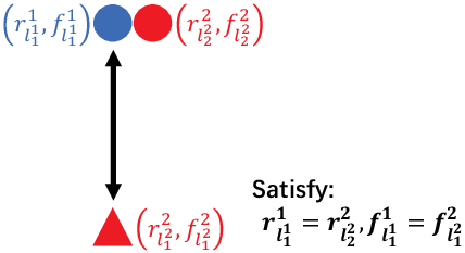
Suppose that (with fusion weight ) consists of a single BC and (with fusion weight ) consists of two BCs, where as shown in Fig. 2. Note that this situation could happen when both tracks in and in are miss-detected. In practice, it is desired to match with , i.e. , due to the fact that and are located at the same position. However, mismatching happens when
| (50) |
where represents a Bernoulli distribution with probability and denotes the Chernoff -coefficient defined as [45]
| (51) |
with the integral replaced by summation when and are defined over a discrete space (e.g. Bernoulli distribution). The proof of (50) is omitted since it can be directly obtained substituting the parameters of BCs into the corresponding definitions. Due to the fact that , and tends to when and are similar, it can be seen immediately that when is extremely low, the right-hand-side of (50) will be close to , which means that mismatching might happen when there exist miss-detections among agents.
Therefore, in this subsection, we propose to solve the label mismatching problem by constructing a modified RAP. Specifically, tye following cost matrix with dimension is defined:
in which the entry represents the cost of assigning the BC of to the BC of . Further denotes the cost of regarding of as unassociated while denotes the cost of regarding of as unassociated. Finally, we artifically set .
Motivated by the above mentioned limitations of GCI divergence, we define the entry as the divergence that considers only the PDF of the BCs, i.e.
where is the matching threshold that represents the largest PDF divergence that the same target could have among agents, and represents an information-theoretic discrepancy among PDFs. There are several candidates that can be adopted to this end, such as:
- -
Jensen-Shannon divergence , which is also known as the symmetric KLD, and is defined as
(58) - -
Cauchy-Schwarz divergence , which is defined as
(59)
Remark 9.
Concerning the computation of information-theoretic discrepancies, the following facts needs to be clarified.
- 1)
When the PDFs of local LMB densities are approximately represented with GMs, the CSD between PDFs can be computed analytically while, on the other hand, the computation of the KLD doe not admit an analyitical form. In the latter case, an approximate solution can be obtained with the aid of a sigma-point representation of the GMs; the details can be found in [46, Appendix A];
- 2)
When the PDFs of local LMB densities are approximately represented with particle sets, both KLD and CSD cannot be accurately computed unless a sufficient amount of particles among the involved PDFs are overlapped. Therefore, in this case, it is suggested to further approximate the particle sets by GMs [41] and then adopt the method discussed in 1).
In order to better illustrate the proposed strategy, it is useful to define the assignment matrix as
where if BC is assigned to and otherwise . Note that, means remains unassigned and similarly that is unassigned; moreover, . Then, the problem turns out to find the best assignment that minimizes the global cost, i.e.
| (63) |
where denotes the trace of a matrix. Such a linear assignment problem can be efficiently solved in polynomial time by the Hungarian algorithm [15, 27].
V-C Application of MIL fusion in the context of DMT
One of the most important applications of multi-object fusion is distributed multitarget tracking (DMT). In this subsection, details of applying MIL fusion to DMT are provided. The considered LRFS approach to DMT considered in this paper consists of the following two steps recursively performed at each time :
- 1)
- 2)
Information aggregation. Based on step 1), local posteriors of all agents are collected at the fusion center (or shared by a broadcast protocol like consensus [47]) and then the multi-object density fusion algorithm is employed to fuse local posteriors , into the global density , and then is utilized as prior information for the local filtering of next iteration at each node .
In the context of DMT, if all agents have the same FoV, fusion can be performed directly with the proposed MIL rule, otherwise local LRFS densities will have to be decomposed into mutually independent sub-densities defined on suitable label subspaces and MIL fusion is performed subspace-by-subspace. If the local FoV of each agent is known, the label subspaces can be obtained at every recursion by looking for the closed region of the global label space. For instance, in the example of Fig. 1, the subspaces could be , , and . However, in practice, it is more desirable to develop fusion rules for agents that have limited but unknown FoVs, due to the facts that:
- -
affected by the physical conditions of the AoI (e.g. rain, fog, etc.), it is hard to precisely define the FoV of each agent;
- -
in some specific MAS like wireless sensor networks (WSNs), the agents are powered by batteries so that as far as energy is consumed, the agent FoV is time-varying.
Notice that if each agent performs well in local filtering, the tracks within its local FoV can be correctly detected after few time recursions. In this sense, it is straightforward to define the label subspaces by comparing the labels that are involved in each local LRFS densitiy (conditioned on the fact that all the local labels have been correctly matched using the method of Section V-B). For instance again in Fig. 2, where involves and while involves and , both local densities contain track and are their respective exclusive tracks. Then it is straightforward to define , , .
Note that, as far as fusion is performed, compensated by local densities of other agents, each agent acquires the information outside its local FoV. As a result, the local label space of each agent includes more and more tracks as far as DMT is implemented. Hence, label subspaces should be re-defined whenever fusion is going to be performed. By considering all the mentioned factors, the proposed DMT approach is outlined in Algorithm 1.
Output:
Remark 10.
Though -GLMB densities can be analytically fused under the MIL criterion, the number of association hypotheses resulting in the global density increases to . Further, the number of association hypotheses of the -GLMB density increases exponentially during local filtering if no additional operation (i.e. pruning of hypotheses) is carried out. As a result, modeling the multitarget state as -GLMB density for DMT requires a huge amount of memory as well as computational resources, thus being practically infeasible. In this regard, for muitarget tracking it is by far preferable to adopt M-GLMB and LMB filters.
Remark 11.
Note that steps of Algorithm 1 are designed for MASs having a fusion center, which is able to exchange information with all the agents. However, this is not always the situation since in some MASs (e.g. WSNs) the agents work in a peer-to-peer (P2P) manner, wherein each individual agent is unable to gather densities from all other agents. In such cases, a promising strategy is the consensus method [48], which consists of iterations of data-exchange with the neighbors and consequent fusion of the received densities with the local one to be performed at each sampling interval. Details on the application of consensus to DMT can be found in [5, 49].
VI Performance evaluation
In this section, simulations concerning DMT over a WSN [50] are carried out in order to assess the performance of MIL fusion. Specifically, two scenarios are considered, where the first one assumes that all the sensor nodes have the same FoV while the second one assumes that the sensing range of each node is limited. Before illustrating the details of simulations, the following statements are in order.
- -
In both scenarios, the MIL rule is combined with M-GLMB and LMB densities, hence the local trackers of [27] and [29] are respectively adopted. The -GLMB density is not considered in the simulations since it requires a huge amount of computational and memory resources as noted in Remark 10, and is therefore unsuitable for WSN applications.
- -
Since the sensor nodes of a WSN are often powered by batteries, their computational ability, memory resources and communication bandwidth are limited. Consequently, all the involved multi-object densities in this section are represented by GMs.
- -
As observed in Remark 11, the sensor nodes of a WSN work in a P2P fashion; hence consensus is employed in the simulations. In particular, we use the algorithm in [49] but replace the “GM-M-GLMB Fusion” step of Table II with the results of Proposition 2 if the multitarget state is modeled as M-GLMB; or the “GM-LMB Fusion” step of Table II with the results of Proposition 3 if the multitarget state is modeled as LMB.
In both scenarios, the single target state at time is denoted as , where and are respectively position and velocity in Cartesian coordinates. It is supposed that the target motion is described by the following linear white noise acceleration model
| (64) |
where represents additive white Gaussian noise with covariance matrix , and
being the sampling interval. Further, it is assumed that each node of the WSN is able to provide both range-of-arrival (ROA) and direction-of-arrival (DOA) measurements of targets, i.e. the measurement generated by a target with state , at time and in node , is modeled as
| (69) |
where is a measurement noise modeled as a zero mean Gaussian process with covariance matrix and
denoting the four quadrant inverse tangent. Clutter at each sensor node has Poisson-distributed cardinality (expected number of targets at each time) and uniform spatial distribution over its local FoV.
The common parameters of local tracks are set as follows: the probability of target survival is set to for all sensor nodes; the Jensen-Shannon divergence (JSD) has been chosen as discrepancy measure for label matching among local densities, with matching threshold . New-born targets are modeled as LMB, where the number of BCs is taken equal to the number of measurements. The EP of each BC is set to and the PDF is taken Gaussian, where the position components of the mean vector are obtained by remapping measurements back to target state space and the velocitiy components are set to zero; the covariance matrix is set to . The pruning and merging thresholds for GMs are set respectively to and . For target extraction, when targets are modeled as M-GLMB, the M-GLMB density is first converted to LMB by matching the PHD and then the tracks with EPs larger than are extracted. At last, whenever local filtering and fusion are accomplished, for M-GLMB densities, label set hypotheses with JEP smaller than and tracks of LMBs with EP smaller than are discarded.
Two performance indicators will be examined in this section: the optimal subpattern assignment (OSPA) distance [51] (with order and cutoff ) and the cardinality estimation error.
VI-A Example 1: DMT with nodes having the same FoV
Let us first consider a simulation scenario wherein targets subsequently enter and then move inside a surveillance region. The considered WSN consists of sensor nodes deployed at known locations for each . The considered scenario is illustrated in Fig. 3.
 |
Now we examine the performance of MIL fusion based on two different probabilities of detection: 1) and 2) for any time and sensor node . The number of consensus steps adopted at each node is set to . In order to better illustrate the performance of MIL fusion, the performance of local trackers without fusion and of local trackers combined with GCI fusion are also considered for comparison.
The average performance over Monte Carlo trials under different detection probabilities ( and ) are illustrated in Figs. 4 and 5 respectively. It can be seen that MIL and GCI fusions provide similar results when the detection probability is high. Conversely, under low detection probability, MIL fusion outperforms GCI fusion especially for target number estimation. Moreover, it is also observed that among MIL fusion based algorithms, the M-GLMB based DMT provides better tracking performance compared to LMB. This fact can be seen more clearly in Fig. 6, where the average OSPA is reported for different probabilities of detection. It can also be seen that, for the M-GLMB model, GCI fusion negatively affects DMT performance when decreases below and, similarly, occurs for the LMB model, when falls below .
 |
 |
 |
VI-B Example 2: DMT with nodes having different FoVs
Next, we consider another scenario wherein the trajectories of targets are the same as in Example 1, while the considered WSN consists of nodes. In this second scenario, the FoV of each sensor node is taken as a circle centred at the node location with radius equal to . In order to provide full coverage of the whole surveillance area, the sensor nodes are regularly placed as shown in Fig. 7. As it can be seen, all targets move to the common FoV of sensor nodes.
 |
Similar to Example 1, we also consider both cases of high () and low () detection probability within the FoV of each sensor. Notice that for each sensor node, we set for targets outside the node FoV. Also in these simulations, the number of consensus steps is set to . The average performance over Monte Carlo trials under different detection probabilities ( and ) are illustrated in Figs. 8 and 9 respectively. It can be seen that MIL fusion is able to detect targets even when they are are in the exclusive FoVs of sensor nodes, while GCI fusion detects targets only when targets are inside the common FoV of sensor nodes. Further, when targets move to the common FoV of sensor nodes, the same conclusions of Example 1 can be drawn.
 |
 |
VII Conclusions
In this paper, a new rule which leads to minimum (weighted) information loss (MIL) is proposed to handle the problem of fusing labeled random finite set (LRFS) densities. An important property of the proposed fusion rule is that, combined with the proposed decomposition strategy of LRFS densities, it can handle the practically relevant case in which local densities are defined in different fields-of-view (FoVs). Further, a strategy is proposed to solve the label mismatching (LM) problem among LRFS densities, thus strengthening the applicability of the proposed algorithms to real problems. The performance of the proposed algorithms is assessed by simulation experiments relative to distributed multitarget tracking (DMT) over a wireless sensor network (WSN).
Appendix A
Appendix B
Proof of Proposition 2.
First, it is recalled from (4) that an M-GLMB density is completely characterized by its JEP and CJPDF . Since the aim is to find the optimal M-GLMB density according to the MIL criterion, it is straightforward to impose a constraint in the optimization problem of (14) as follows
| (73) |
which amounts to directly looking for the JEP and CJPDF characterizing the M-GLMB density . By resorting to the definition of KLD (13) and the permutation invariant property of CJPDF (3), we have (74).
| (74) |
Appendix C
Proof of Proposition 3.
Similarly to (73), the fusion problem with respect to multiple LMB densities can be recast into the following optimization problem
| (76) |
where and are given by (9) and (10) respectively. Specifying the M-GLMB densities as LMB densities, (74) can be further detailed as
| (77) |
where denotes the Bernoulli density with parameter equal to the EP of track , and
| (78) |
Hence (76) is re-written as
| (79) |
Finally, (26) – (27) can be readily obtained by directly applying (15). ∎
Appendix D
If Proposition 2 is adopted to fuse LMB densities, the resulting global density becomes M-GLMB with JEP given by (29) and CJPDF given by
| (80) |
where
| (81) |
Following [29, Section III-B], after converting it to LMB by matching the PHD, the EP of track can be computed as
| (82) |
where
| (83) |
amounts to computing the summation of JEPs of the LMB density defined over all possible label subsets of , thus always equals one, i.e. . Then, it is straightforward to see that . Further, the fused PDF of track is computed as
| (84) |
where represents the inclusion function defined as
Then, it can be seen immediately that the converted LMB density from the fused M-GLMB density is the one obtained by using the results of Proposition 3.
Appendix E
Proof of Theorem 2. The KLD from the fused M-GLMB density of Proposition 2 to the MIL-OFD cannot be directly computed. However, it turns out that it is bounded by [52, eq. (4)]
| (87) |
which proves (31) in Theorem 2. Furthermore, the proof of (32) can be accomplished directly following the steps of (87), and is therefore omitted. ∎
Appendix F
Appendix G
Proof of Proposition 5.
The purpose is to find mutually independent sub-densities defined in disjoint label spaces such that their product minimizes the KL divergence. By definition, we have (89), where denotes the constant that is not related to , . Then. by exploiting the results of Proposition 1 and minimizing , the conclusion of Proposition 5 can be proved.
| (89) |
∎
References
- [1] R. P. Mahler, “Optimal/robust distributed data fusion: a unified approach,” in Signal Processing, Sensor Fusion, and Target Recognition IX, vol. 4052. International Society for Optics and Photonics, 2000, pp. 128–139.
- [2] T. Bailey, S. Julier, and G. Agamennoni, “On conservative fusion of information with unknown non-Gaussian dependence,” in 2012 15th International Conference on Information Fusion. IEEE, 2012, pp. 1876–1883.
- [3] C. Genest and J. V. Zidek, “Combining probability distributions: A critique and an annotated bibliography,” Statistical Science, vol. 1, no. 1, pp. 114–135, 1986.
- [4] M. Üney, D. E. Clark, and S. J. Julier, “Distributed fusion of PHD filters via exponential mixture densities,” IEEE Journal of Selected Topics in Signal Processing, vol. 7, no. 3, pp. 521–531, 2013.
- [5] G. Battistelli, L. Chisci, C. Fantacci, A. Farina, and A. Graziano, “Consensus CPHD filter for distributed multitarget tracking,” IEEE Journal of Selected Topics in Signal Processing, vol. 7, no. 3, pp. 508–520, 2013.
- [6] B. Wang, W. Yi, R. Hoseinnezhad, S. Li, L. Kong, and X. Yang, “Distributed fusion with multi-Bernoulli filter based on generalized covariance intersection,” IEEE Transactions on Signal Processing, vol. 65, no. 1, pp. 242–255, 2017.
- [7] C. Fantacci, B.-N. Vo, B.-T. Vo, G. Battistelli, and L. Chisci, “Robust fusion for multisensor multiobject tracking,” IEEE Signal Processing Letters, vol. 25, no. 5, pp. 640–644, 2018.
- [8] S. Li, W. Yi, R. Hoseinnezhad, G. Battistelli, B. Wang, and L. Kong, “Robust distributed fusion with labeled random finite sets,” IEEE Transactions on Signal Processing, vol. 66, no. 2, pp. 278–293, 2018.
- [9] S. Li, G. Battistelli, L. Chisci, W. Yi, B. Wang, and L. Kong, “Computationally efficient multi-agent multi-object tracking with labeled random finite sets,” IEEE Transactions on Signal Processing, vol. 67, no. 1, pp. 260–275, 2019.
- [10] G. Battistelli and L. Chisci, “Kullback–Leibler average, consensus on probability densities, and distributed state estimation with guaranteed stability,” Automatica, vol. 50, no. 3, pp. 707–718, 2014.
- [11] L. Gao, G. Battistelli, and L. Chisci, “Multiobject fusion with minimum information loss,” arXiv:1903.04239, 2019.
- [12] J. Shore and R. Johnson, “Axiomatic derivation of the principle of maximum entropy and the principle of minimum cross-entropy,” IEEE Transactions on information theory, vol. 26, no. 1, pp. 26–37, 1980.
- [13] J. R. Roy, D. F. Batten, and P. Lesse, “Minimizing information loss in simple aggregation,” Environment and Planning A, vol. 14, no. 7, pp. 973–980, 1982.
- [14] A. E. Abbas, “A Kullback-Leibler view of linear and log-linear pools,” Decision Analysis, vol. 6, no. 1, pp. 25–37, 2009.
- [15] W. D. Blair and Y. Bar-Shalom, Multitarget-multisensor tracking: applications and advances. Artech House, 2000.
- [16] T. Li, J. M. Corchado, and S. Sun, “Partial consensus and conservative fusion of Gaussian mixtures for distributed PHD fusion,” IEEE Transactions on Aerospace and Electronic Systems, 2018.
- [17] T. Li, V. Elvira, H. Fan, and J. M. Corchado, “Local-diffusion-based distributed SMC-PHD filtering using sensors with limited sensing range,” IEEE Sensors Journal, vol. 19, no. 4, pp. 1580–1589, 2019.
- [18] A. K. Gostar, R. Hoseinnezhad, and A. Bab-Hadiashar, “Cauchy-Schwarz divergence-based distributed fusion with Poisson random finite sets,” in 2017 International Conference on Control, Automation and Information Sciences (ICCAIS). IEEE, 2017, pp. 112–116.
- [19] H. G. Hoang, B.-N. Vo, B.-T. Vo, and R. Mahler, “The Cauchy–Schwarz divergence for Poisson point processes,” IEEE Transactions on Information Theory, vol. 61, no. 8, pp. 4475–4485, 2015.
- [20] G. Battistelli, L. Chisci, C. Fantacci, A. Farina, and R. P. Mahler, “Distributed fusion of multitarget densities and consensus PHD/CPHD filters,” in Signal Processing, Sensor/Information Fusion, and Target Recognition XXIV, vol. 9474. International Society for Optics and Photonics, 2015, p. 94740E.
- [21] G. Battistelli, L. Chisci, G. Mugnai, A. Farina, and A. Graziano, “Consensus-based linear and nonlinear filtering,” IEEE Transactions on Automatic Control, vol. 60, no. 5, pp. 1410–1415, 2015.
- [22] G. Battistelli and L. Chisci, “Stability of consensus extended Kalman filter for distributed state estimation,” Automatica, vol. 68, pp. 169–178, 2016.
- [23] M. Üney, J. Houssineau, E. Delande, S. J. Julier, and D. Clark, “Fusion of finite set distributions: pointwise consistency and global cardinality,” IEEE Transactions on Aerospace and Electronic Systems, 2019.
- [24] K. Panta, D. E. Clark, and B.-N. Vo, “Data association and track management for the Gaussian mixture probability hypothesis density filter,” IEEE Transactions on Aerospace and Electronic Systems, vol. 45, no. 3, pp. 1003–1016, 2009.
- [25] F. Papi, B.-N. Vo, B.-T. Vo, C. Fantacci, and M. Beard, “Generalized labeled multi-Bernoulli approximation of multi-object densities,” IEEE Transactions on Signal Processing, vol. 63, no. 20, pp. 5487–5497, 2015.
- [26] B.-T. Vo and B.-N. Vo, “Labeled random finite sets and multi-object conjugate priors,” IEEE Transactions on Signal Processing, vol. 61, no. 13, pp. 3460–3475, 2013.
- [27] B.-N. Vo, B.-T. Vo, and D. Phung, “Labeled random finite sets and the Bayes multi-target tracking filter,” IEEE Transactions on Signal Processing, vol. 62, no. 24, pp. 6554–6567, 2014.
- [28] C. Fantacci, B.-T. Vo, F. Papi, and B.-N. Vo, “The marginalized -GLMB filter,” arXiv preprint arXiv:1501.00926, 2015.
- [29] S. Reuter, B.-T. Vo, B.-N. Vo, and K. Dietmayer, “The labeled multi-Bernoulli filter,” IEEE Transactions on Signal Processing, vol. 62, no. 12, pp. 3246–3260, 2014.
- [30] B.-N. Vo and W.-K. Ma, “The Gaussian mixture probability hypothesis density filter,” IEEE Transactions on Signal Processing, vol. 54, no. 11, pp. 4091–4104, 2006.
- [31] G. Battistelli, L. Chisci, and A. Laurenzi, “Random set approach to distributed multivehicle SLAM,” IFAC-PapersOnLine, vol. 50, no. 1, pp. 2457–2464, 2017.
- [32] M. Vasic, D. Mansolino, and A. Martinoli, “A system implementation and evaluation of a cooperative fusion and tracking algorithm based on a Gaussian mixture PHD filter,” in 2016 IEEE/RSJ International Conference on Intelligent Robots and Systems (IROS). Ieee, 2016, pp. 4172–4179.
- [33] G. Li, G. Battistelli, W. Yi, and L. Kong, “Distributed multi-sensor multi-view fusion based on generalized covariance intersection,” arXiv:1903.06985, 2019.
- [34] X. Wang, A. K. Gostar, T. Rathnayake, B. Xu, A. Bab-Hadiashar, and R. Hoseinnezhad, “Centralized multiple-view sensor fusion using labeled multi-Bernoulli filters,” Signal Processing, vol. 150, pp. 75–84, 2018.
- [35] S. Li, G. Battistelli, L. Chisci, W. Yi, B. Wang, and L. Kong, “Multi-sensor multi-object tracking with different fields-of-view using the LMB filter,” in 2018 21st International Conference on Information Fusion (FUSION). IEEE, 2018, pp. 1201–1208.
- [36] R. P. Mahler, Advances in statistical multisource-multitarget information fusion. Artech House, 2014.
- [37] S. Kullback, Information Theory and Statistics. Dover, 1997.
- [38] M. Beard, B. T. Vo, and B.-N. Vo, “A solution for large-scale multi-object tracking,” arXiv preprint arXiv:1804.06622, 2018.
- [39] B.-N. Vo, S. Singh, and A. Doucet, “Sequential Monte Carlo methods for multitarget filtering with random finite sets,” IEEE Transactions on Aerospace and Electronic Systems, vol. 41, no. 4, pp. 1224–1245, 2005.
- [40] M. Gunay, U. Orguner, and M. Demirekler, “Chernoff fusion of Gaussian mixtures based on sigma-point approximation,” IEEE Transactions on Aerospace and Electronic Systems, vol. 52, no. 6, pp. 2732–2746, 2016.
- [41] T. Li, V. Elvira, H. Fan, and J. M. Corchado, “Local-diffusion-based distributed SMC-PHD filtering using sensors with limited sensing range,” IEEE Sensors Journal, vol. 19, no. 4, pp. 1580–1589, 2018.
- [42] B. Ristic, D. Clark, B.-N. Vo, and B.-T. Vo, “Adaptive target birth intensity for PHD and CPHD filters,” IEEE Transactions on Aerospace and Electronic Systems, vol. 48, no. 2, pp. 1656–1668, 2012.
- [43] A. F. Garcia-Fernandez, “Track-before-detect labeled multi-Bernoulli particle filter with label switching,” IEEE Transactions on Aerospace and Electronic Systems, vol. 52, no. 5, pp. 2123–2138, 2016.
- [44] H. W. Kuhn, “The Hungarian method for the assignment problem,” Naval Research Logistics Quarterly, vol. 2, no. 1-2, pp. 83–97, 1955.
- [45] F. Nielsen, “Chernoff information of exponential families,” arXiv:1102.2684, 2011.
- [46] L. Gao, G. Battistelli, L. Chisci, and P. Wei, “Event-triggered consensus Bernoulli filtering,” in 21st International Conference on Information Fusion (FUSION). IEEE, 2018, pp. 84–91.
- [47] L. Xiao, S. Boyd, and S.-J. Kim, “Distributed average consensus with least-mean-square deviation,” Journal of Parallel and Distributed Computing, vol. 67, no. 1, pp. 33–46, 2007.
- [48] L. Xiao, S. Boyd, and S. Lall, “A scheme for robust distributed sensor fusion based on average consensus,” in IPSN 2005. Fourth International Symposium on Information Processing in Sensor Networks, 2005. IEEE, 2005, pp. 63–70.
- [49] C. Fantacci, B.-N. Vo, B.-T. Vo, G. Battistelli, and L. Chisci, “Consensus labeled random finite set filtering for distributed multi-object tracking,” arXiv:1501.01579, 2015.
- [50] S. C. Mukhopadhyay and H. Leung, Advances in wireless sensors and sensor networks. Springer, 2010, vol. 64.
- [51] D. Schuhmacher, B.-T. Vo, and B.-N. Vo, “A consistent metric for performance evaluation of multi-object filters,” IEEE Transactions on Signal Processing, vol. 56, no. 8, pp. 3447–3457, 2008.
- [52] M. N. Do, “Fast approximation of Kullback-Leibler distance for dependence trees and hidden Markov models,” IEEE Signal Processing Letters, vol. 10, no. 4, pp. 115–118, 2003.