A General Early-Stopping Module for Crowdsourced Ranking
Abstract
Crowdsourcing can be used to determine a total order for an object set (e.g., the top-10 NBA players) based on crowd opinions. This ranking problem is often decomposed into a set of microtasks (e.g., pairwise comparisons). These microtasks are passed to a large number of workers and their answers are aggregated to infer the ranking. The number of microtasks depends on the budget allocated for the problem. Intuitively, the higher the number of microtask answers, the more accurate the ranking becomes. However, it is often hard to decide the budget required for an accurate ranking. We study how a ranking process can be terminated early, and yet achieve a high-quality ranking and great savings in the budget. We use statistical tools to estimate the quality of the ranking result at any stage of the crowdsourcing process, and terminate the process as soon as the desired quality is achieved. Our proposed early-stopping module can be seamlessly integrated with most existing inference algorithms and task assignment methods. We conduct extensive experiments and show that our early-stopping module is better than other existing general stopping criteria. We also implement a prototype system to demonstrate the usability and effectiveness of our approach in practice.
Index Terms:
Crowdsourcing, Ranking, Early Stopping.I Introduction
Crowdsourcing has been used to address a variety of problems, such as language translation [5], entity matching [38, 35], image labeling [17, 36], and object ranking [15, 20]. These problems, which are typically hard for computers to solve, can be easier for humans. Crowdsourcing leverages both human and machine intelligence to derive a solution (e.g., correct inaccuracies in machine predictions). In this paper, we study the use of crowdsourcing on ranking objects. This approach, which has received a lot of attention from different research communities [28, 7, 20], is particularly helpful when ranking cannot be done objectively. For example, to determine the greatest athletes of all times or the best pictures of a landmark, we could solicit opinions from the crowd and aggregate them to a ranking that maximizes the consensus. In addition, crowdsourced ranking can be used to filter data for subsequent machine learning tasks. For instance, ranking answers to a question posted in a forum and selecting only the top ones can ease the burden of natural language processing.
To conduct crowdsourced ranking, existing solutions typically decompose the ranking process into a set of small and easy-to-answer microtasks, such as pairwise comparisons [41]. The microtasks are then distributed via crowdsourcing platforms, such as Amazon Mechanical Turk (AMT) [1] and FigureEight [2], to crowd workers by offering incentives, e.g., money, reputation, etc. The final ranking is computed by an inference algorithm based on the answers collected from the crowd. Naturally, the ranking accuracy is proportional to the number of collected answers to microtasks, i.e., the total budget paid by the requester.
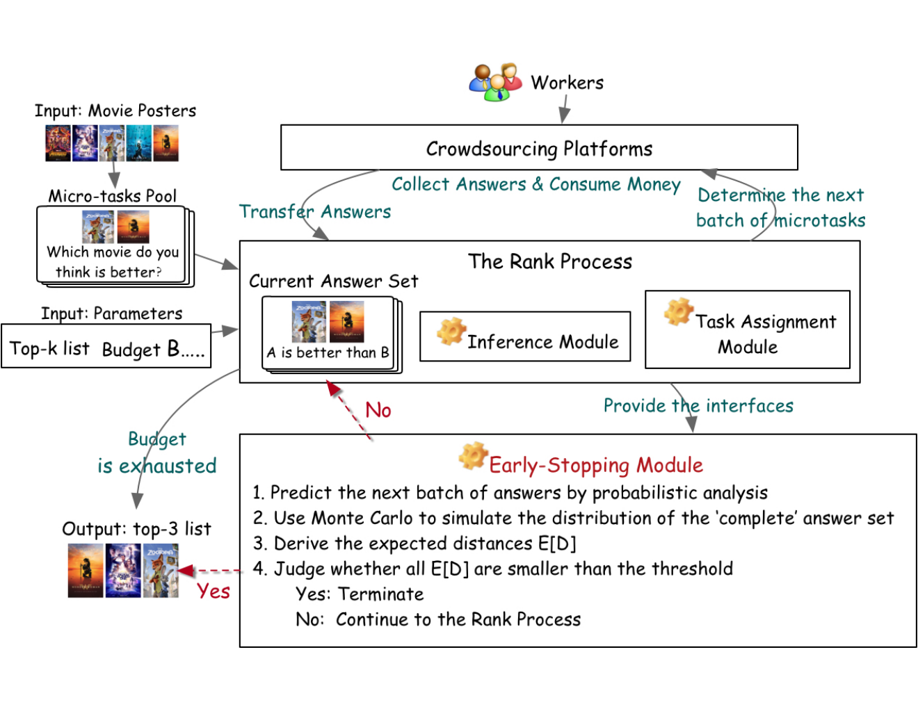
Recent studies [10, 15, 7] attempt to improve the inference algorithm and fine-tune the task assignment (i.e., by dispatching tasks to suitable workers), in order to spend the budget more effectively. Typically, the microtask answers are collected in batches. Let be the th batch of answers; Inference algorithm module infers the interim ranking from ; Task assignment module is used to determine the next batch of microtasks and assign them to crowdsourcing platforms. Fig. 1 illustrates this ranking process .
According to a recent experimental survey on crowdsourced ranking [41], there is no single winner method that outperforms all others in all performance factors (accuracy, convergence rate, efficiency, scalability). In addition, most approaches require the budget to be set in advance, but they offer no guideline on how to set this value. Hence, it is expected that the requester sets a large enough budget, hoping that the ranking process will converge to a stable ranking. This raises an interesting question: can we spend less and achieve approximately the same ranking, as if we had spent all the budget?
To answer this question, we first investigate how much budget could be saved when some representative inference algorithms are applied, i.e., Copeland [29], CrowdBT [10], Iterative [15], and Local [15]. Details about these methods are given in Sec. IV-A. We carry out the ranking and top- query tasks on two public datasets, namely peopleAge [41] and peopleNum [19]. Fig. 2 shows how the accuracy of these algorithms varies as the budget increases. As an accuracy measure, we utilize Kendall’s tau distance between the rankings progressively inferred and the ground truth ranking. All methods converge to a stable state11 1 A formal definition of the stable state is provided in the Sec. II-B., where the change of the distance induced by the inferred ranking is very small. In Fig. 2(a) and (b), CrowdBT reaches a stable state after using just 40% of the budget, whereas all other methods converge when 60% of the budget is used. Similarly for ranking in Fig. 2(c) and (d), the distance changes are all smaller than 0.02 after using 50% of the budget. Obviously, we can stop early the crowdsourcing process when we reach a stable state. We now face the following challenge: how do we know whether the ranking process has reached a stable state?
To tackle this challenge, we develop a novel Early-Stopping (ES) module that attempts to predict the next batch of answers by probabilistic analysis. We then use Monte Carlo simulation [25], based on the prediction model, to construct the distribution of the final answer and, in turn, derive the expected accuracy of the final state. This helps us to assess when the ranking process reaches its stable state, subject to a budget . To early-stop the process, our ES module requires an accuracy tolerance parameter, i.e., the acceptable accuracy that we can afford to lose when compared to the ranking that will be obtained if all the budget is used up.
Our ES module can seamlessly be used by most ranking processes with minimal effort. The only requirement is that the process provides interfaces for the inference and task assignment modules, and accepts a programming call to terminate the crowdsourcing process, when our module determines that the expected accuracy already satisfies tolerance . We emphasize that the development of our ES module is orthogonal to that of inference algorithms and task assignment methods.
The main contributions of this paper are summarized as follows:
- •
To the best of our knowledge, we are the first to propose a general Early-Stopping (ES) module for crowdsourced ranking.
- •
Our ES module is orthogonal to any inference algorithm or task assignment method, and does not interfere with the flow of the crowdsourced ranking process.
- •
We thoroughly evaluate our ES module with subjective and objective tasks, different inference algorithms and task assignment methods, varying budgets and accuracy tolerances. Our module can save even half of the budget given to the ranking processes.
- •
We have developed a prototype system and conducted an online experiment in AMT to assess the effectiveness of our ES module.
The rest of the paper is organized as follows. We formulate the problem and provide definitions and notations in Sec. 2. Our ES module is described in detail in Sec. 3. The experimental evaluations are shown in Sec. 4 and online experiments using our system prototype is presented in Sec. 5. We discuss related work in Sec. 6 and conclude in Sec. 7.
II Preliminaries
We first define crowdsourced ranking and top- queries as follows.
Definition 1 (Crowdsourced Ranking)
Given a set of objects , use human workers to decide a total order .
Definition 2 (Crowdsourced Top- Query)
Given a set of objects , use human workers to find a ranked list of size , such that for any , .
Note that the operator is a conclusion drawn from the crowd’s answers. For instance, given some replies to a question posted in a forum, we can ask the crowd to conduct pairwise comparisons between the replies, and then use existing inference algorithms to process the crowd’s input and find the top-5 replies. Note that comparing two replies is not machine friendly since it not only requires strong natural language processing techniques but also a good understanding of the question, i.e., domain expertise.
II-A Distance Between Rankings
In our solution, we need to measure the distance (i.e., difference) between the ranking inferred at an intermediate state and the ranked list at the final state. To measure the distance between two rankings, a common practice is to use Kendall’s tau distance, i.e., the number of inverse pairs of objects.
We use the normalized Kendall’s tau distance for complete rankings and top- ranked lists as defined in Eq. 1 and Eq. 2, respectively:
| (1) |
| (2) |
where is the indicator function that equals to 1 when its predicate is true, or 0 otherwise. When and are reversed, the numerator of Eq. 1 takes its maximum possible value , and Eq. 1 reaches the highest value of 1. As for Eq. 2, the numerator takes its maximum value when objects in and have no intersection.
Note that there is a case when both and are in one ranked list (e.g., ), and none of them is in the other list (e.g., ). In this case, we have to guess the position of and in . We select the optimistic attitude, i.e., and are in the same order in both top- lists, and do not impose any penalty in the distance function.
| Notation | Description |
| Inference module | |
| Task assignment module | |
| Rank process containing and | |
| Distance function for rankings | |
| Budget | |
| Accuracy tolerance | |
| Number of tasks in a batch | |
| Answers obtained in the th batch | |
| Rank list calculated by | |
| State after collecting batches of answers | |
| Current answer set / Current rank list | |
| Expected distance between the th & th batches | |
| Mean of sampled distances between the th & th batches |
II-B Stable State & Optimal Stopping Point
Publishing a batch of microtasks into the crowdsourced platform is a common strategy to accelerate the speed of collections. Let be the state after collecting the th batch of answers and is the ranked list at . The stopping module of the crowdsourced ranking algorithm should check whether to stop at each . Without loss of generality, we assume that the budget is the total number of microtasks we plan to publish and the number of microtasks, , is the same in each batch. is the total number of batches needed to collect all answers. We then give a formal definition of the stable state that we mentioned in the Introduction:
Definition 3 (Stable State)
Given the whole collection process and an accuracy tolerance from the requester, is called as a stable state of the process if:
- 1.
- 2.
is a stable state
where and .
The first condition secures that the distances between the rankings at any two states (from to the final) do not exceed . The second condition secures the maximality that no earlier (better) stable state can be found in the entire process. It is obvious only one stable state exists in each collection process.
The stopping point is the moment decided by a stopping criterion (SC) to early stop the ranking process. Based on the stable state definition, we can say that
Corollary 1 (The Optimal Stopping Point)
The optimal point to early stop a ranking process is when the process turns into the stable state, i.e., .
The optimal stopping point guarantees the optimality because it saves up as much as possible the budget and ensures the distances from the ranked list at the stopping point to the final ranking are always smaller than the accuracy tolerance .
For example, Fig. 3(a) shows the distance between the current and the final ranking at all states of the process. We show two optimal stopping points with or . Basically we may save more budget with larger . Here we save budget for , and budget for .
One may wonder whether some simple method, e.g., Moving Average [3], can find . We show two kinds of intervals in Fig. 3(b), which has the same distance curve as Fig. 3(a). The first purple rectangle is an interval that tends to be stable during a certain time but descends gradually as more budget consumes. The second one also tends to be stable but the change of rankings is larger than as more budget consumes. Given a current point , moving average uses the previous rank lists in a certain window size to represent the inferred rankings in the future. It is easy to drop out into these intervals and cause the process to stop earlier than it should. To avoid stopping at these intervals, we propose a novel ES module that attempts to discover the optimal stopping point. Table I shows the notations used in this paper.
III Early-Stopping Module
We first discuss how to predict the next batch of answer set by probabilistic analysis. To estimate the final state of the ranking, we use the Monte Carlo method to generate the different possible worlds of the complete answer sets, estimate the expected distances and judge whether stop or not.
III-A Predicting the Next Answer Set
Consider a crowdsourcing rank process , based on an inference module and a task assignment module , that has already collected the th batch answer set (). We predict the next batch of answers by a three-stage process, including (1) determining new tasks , (2) predicting the answers of , and (3) estimating the influence of worker reliability to the answers .
III-A1 Determining new tasks,
Recall that the microtasks of crowdsourced ranking are pairwise comparisons . Given the collected answer set , the task assignment module decides the importance of tasks. The most important tasks are distributed to crowdsourcing platforms as the next batch. We predict answers for these tasks in our subsequent prediction model.
III-A2 Predicting the answer,
Given the collected answer set and a chosen task , we want to predict the answer to . We assume that the workers are reliable since they have to obey the crowdsourcing platform policy, e.g., gain reputation via user feedback. Thereby, we can regard the answer of the task as a Bernoulli distribution of the probability of , denoted as . Formally:
| (3) |
where is the probability of . Several models for has been suggested in previous crowdsourcing studies [24, 6, 33]. For instance, the Bradley-Terry (BT) model [6] defines , where is the latent score of object . The Thurstonian model [33] defines , where is the normal cumulative distribution function. However, some inference modules [13, 12] do not build on the latent scores of objects.
We attempt to design a new estimation model that is suitable for most inference modules. We estimate the probability independently, i.e., only based on the previous answer set of the task . Suppose that the current answer set is ; we build an observed matrix , where is the number of answers reporting in . depends on and .
We use maximum a posteriori probability (MAP) to calculate :
| (4) | ||||
If we assume the prior distribution of as which is the conjugate prior for the Bernoulli distribution, the posterior distribution of is
| (5) |
The reason behind using is that we believe that we have equal probability to get either or . It could also be interpreted as Laplace smoothing to avoid some undefined calculation, e.g., .
The MAP of equals the mode of the posterior distribution, which is
| (6) |
Alternatively, we could also use maximum likelihood estimate (MLE) to calculate :
| (7) | ||||
The MLE of equals to . Similarly, if we replace and by and , respectively, by the Laplace smoothing, then the MLE equation will be identical to Eq. 6 (from MAP).
In summary, we estimate from based on and then sample an answer by for the task .
III-A3 Estimating the influence of worker reliability
In this section, we discuss how worker reliability influences the predicting process of answer . As mentioned in Sec. III-A2, the posterior distribution can be estimated based on the collected answers . The estimation framework is built on our underlying assumption that every worker is reliable.
We relax this assumption and attempt to add the effect of workers’ reliability (i.e., the probability of answering correctly) based on their provided answers in the past. We first define that is the average accuracy of answers in . Assume that the new task is assigned to an unknown coming worker; the probability of answer should be revised as follows:
| (8) |
We use the average reliability of workers already answering to estimate the reliability of coming workers. Note that we can also use the quality of a worker which is recorded in the platforms and calculated by platforms based on workers’ answer history in other projects. But we cannot ask platforms the exact quality of a worker when he/she answers our tasks. Instead, we set a lower bound of the quality to filter bad workers and use this lower bound as for coming workers.
III-A4 Generating answers in the next batch
So far, we have discussed how to predict the next task answer based on the collected answers and worker reliability. To predict the answers obtained in the next batch, we apply an iterative process that generates answers one after another. Algorithm 1 shows the pseudo code of the iterative process. We first estimate in line 2-6. Then we utilize the assignment module to get the importance of tasks. We select the first important tasks, predict the answers respectively and add into in line 7-12.
We can also predict a “complete” answer set (obtained when we use up the budget ). Based on Algorithm 1, we predict based on . Similarly, is predicted based on , is predicted based on and so on. Finally, we can predict until the size of is equal to the given budget .
2
Built matrix based on the answer in 3
6
10
III-B Calculating Deviation
In the last section, we showed how to predict a “complete” answer set . In this section, we discuss how to judge whether the current point satisfies the definition of the optimal stopping point.
III-B1 Expected distance between rankings
Given a deterministic answer set , the inference module can be used to compute the interim ranking and the distance between two rankings (cf. Eq. 1 and 2). However, the probabilistic process may create many possible worlds, i.e., many possible answer sets . If we know the occurrence probability of each possible world where , the expected distance between the th and th batches can be defined as
| (9) |
However, it is difficult to calculate the occurrence probability because it is impossible to conduct a brute-force search for all possible worlds. To tackle this problem, we apply the Monte Carlo method, that allows an estimation of the sampling distribution of almost any statistic using random sampling method. The Monte Carlo method helps to generate a list of possible worlds, i.e., “complete” answer sets . Given a pair , we are able to compute a list of pairs of rankings , and the corresponding distances . By the law of large numbers, the expected distance can be approximated by taking the sample mean
| (10) |
If is the earliest point satisfying , , is the stopping point decided by our ES module.
III-B2 The number of required samples
In the Monte Carlo method, it is important to decide the number of required samples such that the quality is secured. Following common practice, we use Hoeffding’s inequality[16] to decide it.
Hoeffding’s Inequality. Let be independent random variables bounded by the interval . Define the mean of these variables as . Then
| (11) |
where .
We regard a possible world answer set as a sample. The distance can be regarded as an independent random variable given . Based on Hoeffding’s Inequality, we have . This inequality could be transformed into a confidence interval of :
| (12) |
where is computed using Eq. 10. We require at least samples to acquire -confidence interval for .
Given the targeted accuracy tolerance , if we find that , we can also derive We summarize it as the following theorem.
Theorem 1
Given two points and , we secure that with confidence after we random sample “complete” answer sets and find , for some .
Here we set the confidence level and the estimation error as an order of magnitude smaller than which secures enough samples to give a good estimation. We need to sample for , and when we set . The workload of sampling can be accelerated by multithreading or distributed computation.
We then analyze the number of samples to secure all with high probability from the current to the final state, i.e., judge whether the following formula holds: ,
Assume that number of batches for remaining budget is , there are different expected distances needed to compute and check. If we acquire confidence for all the expected distances, the confidence and the number of samples for each expected distance can be set as:
| (13) | |||
| (14) |
We utilize the union bound to prove Eq. 13. Let for a pair be an event. The confidence means the probability that one event fails is . Then based on the union bound, we derive that the probability that at least one of the events fails is no greater than the sum of the probabilities of the individual events, which is using Eq. 13. In other words, the probability that no event fails is at least , which satisfies our requirement.
III-C Putting it all together
In this section, we put all of these techniques together to finalize the ES module, as shown in Algorithm 2. We first calculate how many batches we need to predict the remaining budget (in line 2) and estimate the number of needed samples by Hoeffding’s Inequality (in line 2). During each sample, we use our probabilistic model in Sec. III-A2 to predict a new batch of answers and repeat times to obtain a complete answer set (in lines 2-2). The temporary answer set is current answers we “collect” including actual answers and predicted answers. We record the inferred ranked list after predicting the th batch of answers. At the end of th sample, we know all the ranked lists and compute the distance between the th and th batches.
We then calculate as the expected distance for each remaining batch (in lines 2-2), which is the mean of sampled distances between the interim ranked lists and in the stopping points and . We invoke a programming call to terminate the rank process when the expected distances fulfill the accuracy tolerance (in lines 2-2).
Estimate the number of samples by Eq. 13
Initialize distance array and 2
Create a temporary array of ranked lists and set
for do 4
9
IV Experimental Evaluation
In this section, we thoroughly evaluate our ES module on two real public datasets, which are already collected by others in AMT. Based on the different inference algorithms and task assignment approaches, we compare our ES module with some standard quality estimation methods. The source code and datasets used can be found in https://www.dropbox.com/sh/lp0vu57h13oir33/AACSCYZPOcV33bJSFW6bx85ca?dl=0.
IV-A Experimental Settings
Datasets. We use two real public datasets collected in AMT.
- •
PeopleNum [19] concerns 39 images taken in a mall, each of which includes multiple persons. The goal is to find the images with the most people in them. 6066 answers were collected from 197 workers. Each pair of images is answered by at least 5 workers.
- •
PeopleAge [41] has 50 human photos with ages from 50 to 100. The goal is to find the photos that include the youngest person. There are 4930 answers from 150 workers. Each pair of photos is answered 3 times at least.
PeopleAge is hard because it is relatively subjective and different workers may have different opinions on age. The difficulty of PeopleNum is medium because it costs some time to count the persons.
Inference Modules . According to [41], we select some recommended inference algorithms and task assignment strategies to work with our ES module. For rank inference algorithms, we choose 4 methods:
- •
Copeland is a basic election approach where the objects are sorted by the times they win/lose in the comparisons.
- •
Local is a heuristic-based method based on a comparison graph, where nodes are objects and edges are built based on the pairwise comparisons. The score of an object is defined by the number of winning objects minus the number of losing objects in its 1-hop and 2-hop neighborhood.
- •
Iterative is an extended version of local supporting top- queries. It keeps discarding the bottom half of the objects in the inference process and then re-computes the scores of the surviving objects. It repeats these two processes until objects are left.
- •
CrowdBT is a representative method that uses the Bradley-Terry (BT) model to estimate the latent score of the object . It models the probability as . Based on the crowdsourced comparisons , it computes scores for the objects by maximizing .
Task Assignment Modules . We implemented 4 task assignment strategies based on commercial systems and existing work.
- •
Random is the strategy used by Amazon Mturk; tasks are assigned to coming workers at random and all tasks are answered the same number of times.
- •
Greedy chooses the pair of objects with the highest product of scores as the next task.
- •
Complete finds the top- objects with the highest scores, where is the largest integer satisfying , and sets their pairwise comparisons as the next tasks.
- •
CrowdBT is an active learning method which selects the pair of objects which maximizes the information gain based on the estimated scores.
Based on the characteristics of the inference algorithms and the task assignment strategies, we form and test 7 rank processes : Copeland-Random, Iterative-Random, Local-Random, CrowdBT-Random, Local-Greedy, Local-Complete, and CrowdBT-CrowdBT.
Competitors. In order to evaluate our ES module, we also investigate two alternative stopping criteria based on statistical analysis.
- •
Moving Average (MA) stops when the following equation is smaller than the threshold at the first time. We calculate the distances between all pairs of consecutive rankings or top- lists, generated at the last points before the current stage and average them. Suppose we already collected batches of answers:
(15) - •
Weighted Moving Average (WMA) is similar to MA, except that we assign different weights to the distances based on how far away they are from the current stage. The distance between the latest two rankings has the largest weight , the second latest , etc, and so on.
(16)
Evaluation Metrics. We define the optimal stopping point in the Sec. II-B. To evaluate the effectiveness of different stopping criteria, we analyze the difference between and the stopping point predicted by a stopping criterion. Mathematically:
| (17) |
However, cannot reveal all performance factors of different early-stopping strategies. The stopping point is actually a trade-off between the budget used and the accuracy. If stops ahead of , then this strategy saves more budget but loses accuracy (as the ranked list will be inferred based on fewer answers). To better reveal the real performance of different strategies, we also calculate the percentage of the used budget and the actual error, where
| (18) | ||||
IV-B Experimental Results
IV-B1 Implementation details
We compare our ES module with two competitors, MA and Weighted MA, on two datasets for ranking or top- queries. The objective is to show the superiority and robustness of ES on top of different rank processes .
The total budget is set to the number of answers in each original dataset. The number of microtasks in a batch is set to 200. To get an answer of a microtask , we randomly sample an answer from the answer set of without replacement. If some pairs are running out of answers, we will simulate the next answer by a worker that has average reliability. To solve the cold-start problem of some task assignment strategies, we pre-generate an answer to every pairwise comparison (microtask).
We also choose the best window size for MA and Weighted MA, which is 20 for PeopleNum dataset and 10 for PeopleAge dataset, respectively. Besides, a little change of initial answers for the cold-start problem will change the next sequence of microtasks. Thus, we run the collection process 10 times, and report the average performance.
We use two y-axes in Fig. 4 - 7. The left y-axis is , which is defined in Eq. 17. The right y-axis is the relative stopping point of MA, Weighted MA, ES and the optimal stopping point, which divided by the maximum possible stopping point, . Table II and III show the used budget and actual error for the optimal stopping point and the stopping point decided by ES and Weighted MA averaging by the seven rank processes .
IV-B2 Top- ranking
Fig. 4 and 5 show and the stopping point of our ES module and the two alternative stopping criteria for top- queries. Each stopping criterion is evaluated with seven rank processes (cf. Sec. IV-A). We set by default. The accuracy tolerance is set to , , , . For instance, means the possible number of inverse pairs between the current ranked list and the final state is smaller than .
ES outperforms the other two competitors for different rank processes and different datasets in all settings except for Local-Complete when on PeopleAge dataset. When we set to a larger value (accepting higher accuracy loss), MA and Weighted MA tend to fall into the false states mentioned in the Sec. II-B and stop much earlier than the optimal stopping point, which results in high accuracy loss.
According to the right y-axis, the position of varies from 0.5 to 0.9. The stopping point of our ES module is very close to when compared with the stopping points of MA and Weighted MA. This reveals that ES is effective in finding .
Table II shows the average used budget and the actual error of the optimal stopping point, ES and Weighted MA. Weighted MA always stops earlier rendering the actual error larger than desired. The maximum actual error of Weighted MA is more than 3 times larger than , while ES has an error less than 1 times larger than .
IV-B3 Complete Ranking
Fig. 6 and 7 show the performance for ranking queries. The accuracy tolerance is set to , , , . Note that we exclude two inference algorithms, Iterative and Complete, since they are designed for top- queries.
Similar to top- queries, our ES module is much better than the other two competitions in terms of . The curve of ES’s stopping point is very close to that of compared with MA and Weighted MA. In Table III, the maximum actual error of Weighted MA is more than 4 times larger than while the maximum actual error of ES is less than 2 times larger than .
IV-C Parameter Analysis
In this section, we test the effect of some parameters, including in top- queries, the total budget and the number of microtasks in one batch . We evaluate these parameters with two rank processes, Local-Random and Local-Greedy on PeopleNum dataset.
Fig. 9 shows the effect of in top- queries and Fig. 9 shows the effect of . In these experiments, we set the budget equal to the total number of answers in the original dataset and set . ES is the clear winner since its is always less than or equal to 0.2 and outperforms MA and Weighted MA. In addition, MA and Weighted MA perform worse when becomes small (i.e., fewer microtasks in a batch) or when is large, which means that the distance between two consecutive batches does not represent the distance between the current state and the final state.
Fig. 10 evaluates the effect of the budget . Note that we use the absolute number of answers instead of a percentage in the y-axis. We set and as default. We try , , and for the budget. of ES is always smaller than the corresponding of MA and Weighted MA. Particularly, errors of MA and Weighted MA increase dramatically when increases in Local-Random. This is because increasing budget B improves the quality of the final result and the position of the optimal stopping point moves backwards. But the stopping points predicted by MA and Weighted MA do not change.
| Top-k List | PeopleNum Dataset | PeopleAge Dataset | |||
| UB | AE | UB | AE | ||
| Optimal | 88% | 0.000 | 94% | 0.000 | |
| ES | 87% | 0.003 | 95% | 0.002 | |
| WMA | 54% | 0.007 | 96% | 0.004 | |
| Optimal | 77% | 0.008 | 88% | 0.006 | |
| ES | 78% | 0.009 | 92% | 0.005 | |
| WMA | 57% | 0.027 | 84% | 0.016 | |
| Optimal | 66% | 0.018 | 82% | 0.015 | |
| ES | 58% | 0.028 | 82% | 0.019 | |
| WMA | 26% | 0.052 | 49% | 0.068 | |
| Optimal | 54% | 0.024 | 77% | 0.024 | |
| ES | 45% | 0.038 | 74% | 0.031 | |
| WMA | 20% | 0.055 | 36% | 0.089 | |
| Ranking | PeopleNum Dataset | PeopleAge Dataset | |||
| UB | AE | UB | AE | ||
| Optimal | 95% | 0.002 | 95% | 0.003 | |
| ES | 92% | 0.004 | 96% | 0.003 | |
| WMA | 91% | 0.006 | 96% | 0.001 | |
| Optimal | 89% | 0.006 | 90% | 0.007 | |
| ES | 82% | 0.015 | 88% | 0.010 | |
| WMA | 60% | 0.035 | 61% | 0.029 | |
| Optimal | 83% | 0.013 | 85% | 0.011 | |
| ES | 70% | 0.027 | 81% | 0.019 | |
| WMA | 29% | 0.065 | 35% | 0.051 | |
| Optimal | 79% | 0.016 | 80% | 0.017 | |
| ES | 61% | 0.033 | 72% | 0.028 | |
| WMA | 19% | 0.067 | 31% | 0.057 | |
V Online Experiments In Prototype Systems
To show the effectiveness in practice, we designed an online crowdsourcing system that collects microtask answers from real workers.
V-A Prototype System
Fig. 12(a) - 12(c) show the interface of our prototype, which follows the website style of AMT. Requesters create a new task using the form shown in Fig. 12(a). They can write down the title and descriptions of tasks, upload the objects, choose specific aggregation, assignment and early-stopping modules and set the corresponding parameters. We provide four default aggregation methods (Copeland, Iterative, Local and Crowdbt) and four default assignment methods (Random, Greedy, Complete and Crowdbt). After setting up the problem, requesters obtain IDs for the tasks and corresponding microtask links; see for example Fig. 12(b). Requesters can either post the microtask links on a commercial platform (e.g., AMT) or simply distribute the microtasks to volunteers via a local platform.
After collecting a part of answers, requesters can download the current answer set, obtain the inferred results, and see the curve for the predicted expected distance between the current result and the final result, as shown in Fig. 12(c). The plot is drawn by Python and each point is the expected distance between the inferred ranking after each batch and the final result when the budget is exhausted. We use solid (dotted) line before (after) the current point.
Besides creating a new task and asking workers to answer, our system also provides an interface that allows to upload collected answer set and analyze the performance by tuning different parameters in Fig. 12(a). Similarly, users can see the inferred results and their expected distance in the form of Fig. 12(c).


V-B Local System Experiments
In our local system, we attempt to rank top-5 movies among 10 popular ones, such as Zootopia and Ready Player. Each microtask asks a worker to select the better one between two movies. To run the inference model, we set the default budget to 300 and the number of microtasks in a batch to 20. Our experiments invite 18 volunteers to participate. Our system dispatches microtasks and infers ranking by seven assignment and inference models Copeland-Random, Iterative-Random, Local-Random, CrowdBT-Random, Local-Greedy, Local-Complete, and CrowdBT-CrowdBT. As different worker sequences and reliability distributions may affect the performance, we ran each assignment method 5 times so that we obtained 35 answer curves in total.
We calculated the optimal stopping point and the stopping point decided by MA, Weighed MA and ES for these distance curves. We set the window size of MA and Weighed MA to and to 0.1 and 0.05. Fig. 11(a) and (b) show and the stopping point in different situations. ES’s is always smaller than those of MA and Weighted MA. Moreover, ES’s stopping point is also always closer to the optimal stopping point.
V-C Amazon Mturk Experiments
We also ran the same experiments on Amazon Mechanical Turk (AMT). We attach the link of our local system in the microtasks and we pay for 5 pairwise comparisons. A worker is qualified to answer the microtasks only if her HIT approval rate is greater than . We ran the seven assignment and inference models 3 times and obtained 21 distance curves.
Similar to the experiment in Sec. V-B, we test different stopping criteria when the window size is and the accuracy tolerance is or . Fig. 11(c) and (d) show and the stopping point in different situations. ES’s is smaller than those of MA and Weighted MA in most cases except for Crowdbt-Random when . Compared with MA and Weighted MA, ES is closer to the optimal stopping point on average.
VI related work
In this section, we review the related work from two categories: crowdsourced ranking and early-stopping strategies for crowdsourcing.
Crowdsourced ranking. The ranking problem has a long history and has been studied in the past several decades. Simple traditional ranking algorithms, e.g., BordaCount [4] and Copeland [29], rank objects by the times they win/lose in the comparisons. In the context of crowdsourcing, we also need to consider the fact that the crowd may give incorrect answers (traditional ranking algorithms do not consider possible errors). How to deal with noisy answers and control worker qualities is the key component in almost all crowdsourcing problems [21, 42, 31, 32]. To solve it, inference algorithms have been proposed to infer a ranked list based on the collected (noisy) answers. Moreover, task assignment strategies have been put forward to allocate suitable tasks to high-quality workers and obtain informative answers.
Inference algorithms in raking problems can be divided into two categories: heuristic-based solutions from the DB community approach the problem as a top- operation in databases, and machine-learning algorithms formalize it as a leaning problem and maximize the likelihood of top- objects. Heuristic score-based algorithms [15, 27, 39, 34] rank objects by estimating the underlying score of objects. CrowdBT [10] and CrowdGauss [28] are ML algorithms, which set the objective function based on the assumption and use maximum likelihood to obtain the top- object with the highest probability.
Regarding task assignment strategies, Amazon MTurk follows a random assignment strategy; i.e., microtasks are randomly dispatched to each coming worker. Random assignment does not consider the difficulties of microtasks. Some heuristic assignment methods [15] aim at maximizing the probability of obtaining the top- result, e.g., by selecting most promising object pairs (e.g., with the largest latent scores) to compare. [7] avoids some unnecessary comparisons by setting a bound for the object latent score. Active learning methods are also used in CrowdBT [10] and CrowdGauss [28] to compare objects with the largest expected information gain.
According to a recent experimental study [41], different inference and assignment methods have their own advantages and there does not exist a single best one. Machine-learning methods for answer aggregation typically have high quality. Still, global inference heuristics that utilize global comparison results achieve comparable and even higher quality than ML methods. Local inference heuristics have poor quality, but have higher efficiency and scalability. For task assignment, active-learning methods achieve higher quality than heuristics, but they have low efficiency.
Stopping Criteria. Stopping criteria have been defined for various crowdsourcing problems. [26] and [30] design an early-stopping strategy for multiple-choice-question problems (e.g., choosing the opinion positive, neutral, or negative in a sentence). [40] and [23] use Sequential Probability Ratio Test (SPRT) [37] to decide when to stop for multi-labeling tasks (e.g., labeling pictures as a portrait or a landscape). Besides, [8] uses Chao92 [9] estimator to estimate the level of completion (and the termination point) for entity collection problems (e.g., collecting a set of active NBA players). The settings of all these problems are quite different from crowdsourced ranking. The reason is that microtasks are independent in these problems, while microtasks in ranking problems are correlated.
Previous work on crowdsourced ranking [20] and [11] define stopping conditions in their assignment methods. For instance, [11] assumes that each object has a latent score and answers to pairwise comparisons follow the Bradley-Terry (BT) [6] model. However, this approach cannot be used with methods whose assumption is the Thurstone’s model [33] or Plackett-Luce model [14]. It is also not suitable if the objects do not have scores. [20] asks the crowd to give a numerical answer in for a pairwise comparison and calculates the confidence interval of the result. This approach cannot be applied if the answers are just 0 or 1, and it is based on special assumptions that cannot generalize to most situations.
Moving average and Weighted moving average [3] are to measure the change between two consecutive batches and stop if the change is smaller than a threshold. However, the result may be oscillatory convergent, i.e., it may be stable during a small period of time and then change as the number of answers increases. In this case, they stop earlier than desired. Besides, it is hard for users to set the best parameter values for them, such as the window size. Bad parameters lead to the worst stopping position.
VII conclusion
In this paper, we proposed a general stopping criterion for crowdsourced ranking. The goal is to terminate answer collection as soon as the estimated ranking becomes very similar to the ranking that we expect to obtain when all the budget is exhausted. This way, resources and time for obtaining the result are saved. We demonstrated the robustness of our method in different situations, including subjective or objective tasks, diverse inference modules or task assignment modules and different budget and tolerance parameter values. We implemented a prototype which can be used by requesters in practice.
There are several directions for future work. First of all, although we have only considered pairwise comparisons as microtasks in this paper, our module can also be applied for microtasks where multiple objects are compared by a worker; in this case, we use multinomial distributions instead of Bernoulli distributions. Besides, some inference modules, such as rating-based algorithms[22] and hybrid algorithms[18], are still not suitable for our current module. We will study the extension of our module to predict ratings of objects.
References
- [1] Amazon mechanical turk. https://www.mturk.com.
- [2] Figure eight. https://www.figure-eight.com.
- [3] Moving average. https://en.wikipedia.org/wiki/Moving_average.
- [4] R. M. Adelsman and A. B. Whinston. Sophisticated voting with information for two voting functions. J. of Economic Theory, 15(1):145–159, 1977.
- [5] V. Ambati, S. Vogel, and J. Carbonell. Collaborative workflow for crowdsourcing translation. In Proceedings of the ACM 2012 conference on Computer Supported Cooperative Work, pages 1191–1194. ACM, 2012.
- [6] R. A. Bradley and M. E. Terry. Rank analysis of incomplete block designs: I. the method of paired comparisons. Biometrika, 39(3/4):324–345, 1952.
- [7] R. Busa-Fekete, B. Szorenyi, W. Cheng, P. Weng, and E. Hüllermeier. Top-k selection based on adaptive sampling of noisy preferences. In ICML, pages 1094–1102, 2013.
- [8] C. Chai, J. Fan, and G. Li. Incentive-based entity collection using crowdsourcing. In ICDE, pages 341–352. IEEE, 2018.
- [9] A. Chao and S.-M. Lee. Estimating the number of classes via sample coverage. Journal of the American statistical Association, 87(417):210–217, 1992.
- [10] X. Chen, P. N. Bennett, K. Collins-Thompson, and E. Horvitz. Pairwise ranking aggregation in a crowdsourced setting. In WSDM, pages 193–202. ACM, 2013.
- [11] X. Chen, Y. Chen, and X. Li. Asymptotically optimal sequential design for rank aggregation. arXiv preprint arXiv:1710.06056, 2017.
- [12] S. B. Davidson, S. Khanna, T. Milo, and S. Roy. Using the crowd for top-k and group-by queries. In ICDT, pages 225–236. ACM, 2013.
- [13] B. Eriksson. Learning to top-k search using pairwise comparisons. In Artificial Intelligence and Statistics, pages 265–273, 2013.
- [14] J. Guiver and E. Snelson. Bayesian inference for plackett-luce ranking models. In proceedings of the 26th annual international conference on machine learning, pages 377–384. ACM, 2009.
- [15] S. Guo, A. Parameswaran, and H. Garcia-Molina. So who won?: dynamic max discovery with the crowd. In SIGMOD, pages 385–396. ACM, 2012.
- [16] W. Hoeffding. Probability inequalities for sums of bounded random variables. Journal of the American statistical association, 58(301):13–30, 1963.
- [17] D. R. Karger, S. Oh, and D. Shah. Efficient crowdsourcing for multi-class labeling. SIGMETRICS, 41(1):81–92, 2013.
- [18] A. R. Khan and H. Garcia-Molina. Hybrid strategies for finding the max with the crowd. Technical report, Technical report, 2014.
- [19] A. R. Khan and H. Garcia-Molina. Hybrid strategies for finding the max with the crowd: technical report. Technical report, Stanford InfoLab, 2014.
- [20] N. M. Kou, Y. Li, H. Wang, L. H. U, and Z. Gong. Crowdsourced top-k queries by confidence-aware pairwise judgments. In SIGMOD, pages 1415–1430. ACM, 2017.
- [21] G. Li, J. Wang, Y. Zheng, and M. J. Franklin. Crowdsourced data management: A survey. TKDE, 28(9):2296–2319, 2016.
- [22] K. Li, X. Zhang, and G. Li. A rating-ranking method for crowdsourced top-k computation. In SIGMOD, pages 975–990. ACM, 2018.
- [23] X. Li, Y. Chen, X. Chen, J. Liu, and Z. Ying. Optimal stopping and worker selection in crowdsourcing: An adaptive sequential probability ratio test framework. arXiv preprint arXiv:1708.08374, 2017.
- [24] T. Lu and C. Boutilier. Learning mallows models with pairwise preferences. In ICML, pages 145–152, 2011.
- [25] N. Metropolis and S. Ulam. The monte carlo method. Journal of the American statistical association, 44(247):335–341, 1949.
- [26] L. Mo, R. Cheng, B. Kao, X. S. Yang, C. Ren, S. Lei, D. W. Cheung, and E. Lo. Optimizing plurality for human intelligence tasks. In CIKM, pages 1929–1938. ACM, 2013.
- [27] S. Negahban, S. Oh, and D. Shah. Iterative ranking from pair-wise comparisons. In Advances in neural information processing systems, pages 2474–2482, 2012.
- [28] T. Pfeiffer, X. A. Gao, Y. Chen, A. Mao, and D. G. Rand. Adaptive polling for information aggregation. In AAAI, 2012.
- [29] J.-C. Pomerol and S. Barba-Romero. Multicriterion decision in management: principles and practice, volume 25. Springer Science & Business Media, 2012.
- [30] V. Raykar and P. Agrawal. Sequential crowdsourced labeling as an epsilon-greedy exploration in a markov decision process. In Artificial intelligence and statistics, pages 832–840, 2014.
- [31] C. Shan, N. Mamoulis, G. Li, R. Cheng, Z. Huang, and Y. Zheng. T-crowd: Effective crowdsourcing for tabular data. In 2018 IEEE 34th International Conference on Data Engineering (ICDE), pages 1316–1319. IEEE, 2018.
- [32] C. Shan, N. Mamoulis, G. Li, R. Cheng, Z. Huang, and Y. Zheng. A crowdsourcing framework for collecting tabular data. IEEE Transactions on Knowledge and Data Engineering, 2019.
- [33] L. L. Thurstone. A law of comparative judgment. Psychological review, 34(4):273, 1927.
- [34] P. Venetis, H. Garcia-Molina, K. Huang, and N. Polyzotis. Max algorithms in crowdsourcing environments. In Proceedings of the 21st international conference on World Wide Web, pages 989–998. ACM, 2012.
- [35] N. Vesdapunt, K. Bellare, and N. Dalvi. Crowdsourcing algorithms for entity resolution. PVLDB, 7(12):1071–1082, 2014.
- [36] C. Vondrick, D. Patterson, and D. Ramanan. Efficiently scaling up crowdsourced video annotation. International Journal of Computer Vision, 101(1):184–204, 2013.
- [37] A. Wald. Sequential tests of statistical hypotheses. The annals of mathematical statistics, 16(2):117–186, 1945.
- [38] J. Wang, T. Kraska, M. J. Franklin, and J. Feng. Crowder: Crowdsourcing entity resolution. PVLDB, 5(11):1483–1494, 2012.
- [39] F. Wauthier, M. Jordan, and N. Jojic. Efficient ranking from pairwise comparisons. In International Conference on Machine Learning, pages 109–117, 2013.
- [40] P. Welinder and P. Perona. Online crowdsourcing: rating annotators and obtaining cost-effective labels. In CVPRW, pages 25–32. IEEE, 2010.
- [41] X. Zhang, G. Li, and J. Feng. Crowdsourced top-k algorithms: An experimental evaluation. PVLDB, 9(8):612–623, 2016.
- [42] Y. Zheng, G. Li, Y. Li, C. Shan, and R. Cheng. Truth inference in crowdsourcing: is the problem solved? PVLDB, 10(5):541–552, 2017.