Two-year Cosmology Large Angular Scale Surveyor (CLASS) Observations:
A First Detection of Atmospheric Circular Polarization at Q BandAstropy (Astropy Collaboration et al. 2013; Astropy Collaboration et al. 2018), NumPy (van der Walt et al. 2011), SciPy (Virtanen et al. 2019), Numba (Lam et al. 2015), MSISE-00 (Hirsch 2019), Healpy (Zonca et al. 2019; Gorski et al. 2005), Matplotlib (Hunter 2007)
Abstract
The Earth’s magnetic field induces Zeeman splitting of the magnetic dipole transitions of molecular oxygen in the atmosphere, which produces polarized emission in the millimeter-wave regime. This polarized emission is primarily circularly polarized and manifests as a foreground with a dipole-shaped sky pattern for polarization-sensitive ground-based cosmic microwave background experiments, such as the Cosmology Large Angular Scale Surveyor (CLASS), which is capable of measuring large angular scale circular polarization. Using atmospheric emission theory and radiative transfer formalisms, we model the expected amplitude and spatial distribution of this signal and evaluate the model for the CLASS observing site in the Atacama Desert of northern Chile. Then, using two years of observations at from the CLASS Q-band telescope, we present a detection of this signal and compare the observed signal to that predicted by the model. We recover an angle between magnetic north and true north of , which is consistent with the expectation of for the CLASS observing site. When comparing dipole sky patterns fit to both simulated and data-derived sky maps, the dipole directions match to within a degree, and the measured amplitudes match to within .
Keywords:
Cosmic microwave background radiation (322); Observational cosmology (1146); Polarimeters (1277); Astronomical instrumentation (799); Atmospheric effects (113)I Introduction
In the presence of Earth’s magnetic field, molecular oxygen in the atmosphere experiences Zeeman splitting of its magnetic dipole transitions. This produces polarized emission in the millimeter-wave regime, primarily circular polarization, which manifests as a foreground for polarization-sensitive ground-based cosmic microwave background (CMB) experiments such as the Cosmology Large Angular Scale Surveyor (CLASS) (Eimer et al. 2012; Essinger-Hileman et al. 2014; Harrington et al. 2016). The effect of this foreground has previously been discussed qualitatively by Keating et al. 1998 and quantified by Hanany & Rosenkranz 2003 and Spinelli et al. 2011. However, previous attempts to observe this foreground, such as by Mipol (Mainini et al. 2013), have not been successful in detecting it.
Molecular oxygen has strong emission lines in the range, as well as a line at , which are in the frequency range of interest for CMB observations. There are also water vapor and ozone emission lines near this frequency range, but unlike diatomic oxygen, these molecules do not experience Zeeman splitting and thus do not produce polarized emission (Liebe 1981). Zeeman splitting of molecular oxygen is generally considered in the context of remote sensing of the temperature of the mesosphere, where individual Zeeman-split emission lines can be resolved; pressure broadening obscures individual lines at lower altitudes (Meeks & Lilley 1963).
Modeling of the polarized emission of Zeeman-split oxygen began with the seminal works of Lenoir 1967; Lenoir 1968, with further development of atmospheric emission models by Liebe 1981; Liebe 1989, Liebe et al. 1992; Liebe et al. 1993, Rosenkranz & Staelin 1988, and others. Near the emission lines, both linearly and circularly polarized emission have been detected from orbit (Schwartz et al. 2006; Kunkee et al. 2008). Ground-based detections of linear polarization have also been made at the emission lines, at (Pardo et al. 1995) and (Navas-Guzmán et al. 2015). However, atmospheric remote sensing instruments generally do not observe polarization at frequencies far from the emission lines.
As the circular polarization predicted by standard cosmological models is many orders of magnitude smaller than that of the linearly polarized signal (Inomata & Kamionkowski 2019), CMB experiments are built to be primarily sensitive to linear polarization, which is itself an extremely faint signal (Hu & White 1997). For ground-based experiments, the linearly polarized signal from Zeeman-split molecular oxygen is expected to be on the level, roughly four orders of magnitude weaker than the corresponding circularly polarized signal (Hanany & Rosenkranz 2003). As this is much fainter than can be detected with current CMB instruments and as the circularly polarized component is much stronger, atmospheric Zeeman emission is primarily considered a CMB foreground at the largest angular scales (), fixed in topocentric coordinates, due to potential circular-to-linear polarization leakage as a result of instrument non-idealities (O’Dea et al. 2007). For linear polarization, emission and scattering by ice crystal clouds in the upper troposphere is a larger atmospheric contaminant (Pietranera et al. 2007; Takakura et al. 2019).
For large angular scales at Q band (), diffuse Galactic synchrotron emission is expected to be the largest contributor to extraterrestrial circular polarization, with circular polarization due to Faraday conversion of linear polarization induced by Population III stars exceeding this contribution at smaller angular scales (King & Lubin 2016). Another possible source of Faraday conversion is via galaxy cluster magnetic fields, at primarily small angular scales (Cooray et al. 2003). Beyond synchrotron emission and Faraday conversion, additional potential sources of circular polarization include scattering by the cosmic neutrino background (Mohammadi 2014), primordial magnetic fields (Giovannini 2009), photon–photon interactions in neutral hydrogen (Sawyer 2015), and cosmic birefringence via coupling of the Chern–Simons term (Carroll et al. 1990), as well as postulated new physics (Zarei et al. 2010; Tizchang et al. 2016). As these predicted signals are at most on the level, they are well below current detection thresholds.
The most stringent previously published upper limit on CMB circular polarization was set by the balloon-borne Spider instrument, utilizing non-idealities in its half-wave plate polarization modulators at frequencies near and (Nagy et al. 2017). As Spider observed from the stratosphere, above much of the atmosphere and thus much of the atmospheric emission, it was not sensitive to atmospheric circularly polarized emission. However, for ground-based experiments to significantly improve on this limit, circularly polarized atmospheric emission must first be detected and subtracted. As with Mipol (Mainini et al. 2013), previous ground-based measurements did not have the requisite sensitivity to detect circularly polarized atmospheric emission (Lubin et al. 1983; Partridge et al. 1988). An improved upper limit on extraterrestrial circular polarization utilizing CLASS observations is presented in a companion paper, Padilla et al. 2020.
Through its use of Variable-delay Polarization Modulators (VPMs) (Chuss et al. 2012; Harrington et al. 2018), CLASS is uniquely capable of measuring large angular scale circular polarization. CLASS currently observes the microwave sky in frequency bands centered near , using three telescope receivers; a fourth receiver will be deployed in the future. The present analysis focuses on the first two years of observations from the Q-band telescope, which is centered near . CLASS is designed to map the polarization of the CMB at large angular scales over 75% of the sky to detect or place an upper limit on the B-mode signal of primordial gravitational waves and to measure the optical depth due to reionization, , to near the cosmic variance limit (Watts et al. 2015; Watts et al. 2018).
VPMs utilize a movable mirror placed behind a linearly polarizing array of parallel wires to induce a varying phase delay between polarization states perpendicular to and parallel to the direction of the array wires. When combined with detectors sensitive to linear polarization, modulating the mirror position, and thus the distance between the mirror and the wire array, results in the modulation of one linear polarization state, instrument Stokes in the case of CLASS, into circular polarization, Stokes , and vice versa. This modulation increases polarization measurement stability by utilizing phase-sensitive detection and allows for the measurement of large angular scale modes on the sky. As Stokes and are modulated instead of Stokes and as is the case of half-wave plate modulators more commonly used in CMB instruments (Kusaka et al. 2018), CLASS has significant capability to measure circular polarization (K. Harrington et al. 2020, in preparation). Furthermore, its detection capability is a more direct measurement than sensitivity obtained via half-wave plate non-idealities, which are highly frequency dependent in a poorly constrained manner (Nagy et al. 2017).
The remainder of this paper is organized as follows. In Section II, we present the theory behind polarized Zeeman emission of molecular oxygen in the atmosphere that is used to simulate the expected signal. Next, in Section III, we present the results of these simulations for the CLASS observing site in the Atacama Desert of northern Chile. Then, we compare the simulation results to data from the first era of observations of the CLASS Q-band receiver in Section IV. Finally, we conclude in Section V.
II Atmospheric emission theory
In its electronic ground state, molecular oxygen has a spin quantum number due to the unpaired spins of two electrons, resulting in a magnetic dipole moment. This magnetic dipole moment results in transitions between rotational states of the molecule’s electronic and vibrational ground states with millimeter-wave emission. The spin quantum number couples with the total rotational angular momentum quantum number , which must be odd due to the exclusion principle, to yield the rotational quantum number . This results in three possible values for per , . Selection rules allow for an transition, , and an transition, . In the absence of an external magnetic field, this emission is unpolarized, but a non-zero external magnetic field induces Zeeman splitting, which produces polarized emission (Berestetskii et al. 1982). An external magnetic field splits the transition lines due to a given into lines corresponding to the magnetic quantum number , where ; expresses the projection of the molecular magnetic moment on the external magnetic field vector.
II.1 Layer Attenuation
II.1.1 Molecular Oxygen
In a coherency matrix formalism (Lenoir 1967), the attenuation of a given atmosphere layer due to resonances in molecular oxygen can be defined as
| (1) |
where () is the intensity of the unsplit line, is the transition matrix, is the intensity of the Zeeman component relative to the unsplit line, () is the line profile, () is the frequency of evaluation, and () is the frequency of the Zeeman line. Note that this is field attenuation, which is a factor of two smaller than power attenuation, in units of . The outer summation is performed over the first thirty-eight resonance lines, starting at and ending at . Higher order resonance lines are excluded due to lack of available line broadening and mixing data; as these lines are much weaker, the effect of excluding them is minimal.
The intensity of the unsplit line () is
| (2) |
where () is the fiducial intensity at , is the volume fraction of molecular oxygen in the atmosphere (Machta & Hughes 1970),11 1 This decreases at very high altitudes due to photodissociation (Penndorf 1949), but, as will be shown later, the relevant signal is primarily from the lower atmosphere. is the fractional partial pressure of dry air, () is the pressure of the atmosphere layer, () is the molar gas constant, () is the physical temperature of the atmosphere layer, is a reference temperature, () is the lower-state energy of the transition, and is the Boltzmann constant (). and values are from Hitran (Gordon et al. 2017). As per Liebe et al. 1993, the fractional partial pressure of water vapor is
| (3) |
where is the fractional relative humidity and is a reference temperature.
For ,
| (4) |
and for ,
| (5) |
where is the angle between the line of sight and the geomagnetic field vector and
Thus, the amplitude of circular polarization is maximized when the line of sight is aligned with the direction of the magnetic field, and the linear polarization is maximized when the two vectors are perpendicular.
While the Zeeman effect in molecular oxygen can be approximated to reasonable accuracy by Hund’s case (b) (Townes & Schawlow 1955), we use the more exact calculations laid out in Larsson et al. 2019. In this formalism, the frequencies of the Zeeman lines are given by , where () [from Hitran (Gordon et al. 2017)] is the frequency of the unsplit line and
| (6) |
is the Zeeman frequency shift in . Here, () is the magnetic field strength, () is the Bohr magneton, () is the Planck constant, and and are the numerical Zeeman coefficients corresponding to the given transition from Table 2 of Larsson et al. 2019. The values of the relative intensity factor are shown in Table 1; note that these normalize to two in the absence of a magnetic field, but when combined with , the combination yields the identity matrix.
| line | line | |
|---|---|---|
Note. — For Zeeman components of O2 lines, where (Liebe 1981).
Following Larsson et al. 2014 and Melsheimer et al. 2005 the line profile is defined as
| (7) |
where the Faddeeva function (for ) (Faddeyeva & Terent′ev 1961) is,
| (8) |
with
| (9) |
Here, is the second order line shape correction, is the first order phase correction, and is the second order frequency correction. These are defined with temperature dependence by
| (10) |
where is the first or second order coefficient , , or and (), (), and () are all from Table 1 of Makarov et al. 2011; the exponent is 0.8 for and 1.6 for and . The pressure broadening half width is
| (11) |
for
| (12) |
where (), (), , , and are parameters from column four of Table 3 of Koshelev et al. 2016 for and from column two of Table 2 of Koshelev et al. 2015 for ; the exponent is from Table 1 of Koshelev et al. 2016. Also used is the Doppler half width (Herbert 1974; Varghese & Hanson 1984),
| (13) |
in , where () is the speed of light and () is the molar mass of molecular oxygen [from Hitran (Gordon et al. 2017)]. The factor is a normalization (Armstrong 1967). At high pressures, the Faddeeva function simplifies to a Lorentz shape function, so the combination of the two Faddeeva functions reduces to a Van Vleck–Weisskopf (Van Vleck & Weisskopf 1945) line shape. At low pressures, when , the line mixing and pressure correction effects are eliminated, so the function behaves similar to a Voigt line shape function, although with slightly reduced amplitude on the line wings. As will later be shown, the high pressure case is more important, so the line shape function was chosen such that it is most accurate in that regime.
II.1.2 Dry Air and Water Vapor
While the Zeeman effect is the sole significant non-transient source of polarized atmospheric emission in the millimeter spectrum, there are other unpolarized sources, quantified by a dry air continuum and water vapor contributions. Following Tretyakov 2016, the dry air and water vapor non-resonant continua term is
| (14) |
where , , () and , , are numerical coefficients from from Table 5 of Tretyakov 2016. Following Rosenkranz 1998, the water vapor contribution is
| (15) |
summed over the water vapor lines shown in Table 1 of Rosenkranz 1998, where the line profile is defined as
| (16) |
with
| (17) |
where is a cutoff frequency and , () and , are numerical coefficients from Table 1 of Rosenkranz 1998. This formulation resembles the Van Vleck–Weisskopf line shape but includes a high frequency cutoff, as proposed by Clough et al. 1989. The line intensities, (), follow equation (2) but with replaced with ; () and () values are again from Hitran (Gordon et al. 2017), along with the line frequencies, (). The full coherency matrix () is then
| (18) |
where is the identity matrix.
II.2 Radiative Transfer
As we are interested in polarization, a tensor radiative transfer approach is required to model how radiation propagates through the atmosphere. Using a plane-parallel approximation, the atmosphere is divided into layers of thickness starting from ground level, in the case of CLASS, and ending at ; denotes the zenith angle. Using the approach described in Lenoir 1967; Lenoir 1968 and including phase as per Rosenkranz & Staelin 1988, the brightness temperature coherency matrix (Randa et al. 2008) of a given atmosphere layer is defined as
| (19) |
using matrix exponentiation, where is the brightness temperature coherency matrix of the atmosphere layer before it, () is the physical temperature of the atmosphere layer, and represents the conjugate transpose operation. Since we are observing from the ground, unlike the satellite observations described in Lenoir 1968, we start at with and calculate the propagation downward layer-by-layer until the ground, where is the CMB monopole (Fixsen 2009) brightness temperature at the observing frequency. Note that as the brightness temperature coherency matrix contains matrix elements defined in terms of the brightness temperature of a single polarization of radiation,22 2 See the footnote of Section 1.2.2 of Janssen 1993 for a discussion of differing brightness temperature definitions. there is an extra factor of one half in the conversion to Stokes parameters when compared to a standard coherency matrix (Born & Wolf 1959), e.g., .
II.3 Atmosphere and Magnetic Field Properties
In order to perform the aforementioned calculations, data are needed for the atmospheric temperature and pressure profiles, as well as the geomagnetic field vector direction and magnitude at the location in question. The Nrlmsise-00 atmosphere model (Picone et al. 2002), averaged over the full year, was used to calculate the temperature and pressure profiles used; for the lower atmosphere, this model was compared to data acquired via radiosonde launches from the Chajnantor Plateau, which is adjacent to the CLASS observing site, during the Alma site characterization campaign33 3 Data retrieved from http://legacy.nrao.edu/alma/site/Chajnantor/instruments/radiosonde/. and was found to be in good agreement. The magnetic field was calculated at ground level using the National Oceanic and Atmospheric Administration’s Enhanced Magnetic Model 2017 (EMM2017) (Chulliat et al. 2015). While the magnetic field strength does decrease with altitude, this effect is minor, so it was omitted from the calculations.
II.4 Primary Source of Polarized Emission
Zeeman emission from atmospheric molecular oxygen is generally considered to be a mesospheric effect, since individual emission lines can be discerned at these altitudes due to the lack of pressure broadening. However, we are interested in polarized emission at frequencies far from the resonance lines, where the discernibility of individual emission lines is not relevant. To determine which altitude region of the atmosphere is primarily responsible for the polarized emission, we simulated a series of observations to the north with a zenith angle from the CLASS observing site in the frequency band of the CLASS Q-band telescope; the properties of both the site and telescope are further detailed in the next section. Instead of starting at altitude to calculate the layer-by-layer propagation downward, the starting altitude is reduced incrementally and compared to the fiducial case, the results of which are shown in Figure 1. This series of calculations shows that the lower atmosphere is the primary contributor to the polarized Zeeman emission far from the resonance lines, with three-quarters of the signal contributed by the troposphere. At lower altitudes, the atmospheric pressure is higher, so there are more oxygen molecules per unit volume, which leads to more emission. Thus, while the mesospheric emission is most significant when one wishes to resolve individual Zeeman emission lines, tropospheric emission is most significant far from the resonance lines.
III Simulation results
The CLASS observing site is located at elevation in the Atacama Desert of northern Chile, with coordinates S, W. For this location, at ground level, the EMM2017 magnetic field model was evaluated for 2017 January 1, a date near the middle of the observing period that will be described in Section IV; this resulted in a magnetic field of oriented with an azimuth angle of and a zenith angle of . As previously mentioned, the Nrlmsise-00 atmosphere model was used to calculate temperature and pressure profiles. To include water vapor effects, relative humidity is assumed, which is a typical value for the CLASS observing site during good weather; this corresponds to of precipitable water vapor (PWV). As the observations are made away from the water vapor resonance lines, the relative humidity only affects the polarized signal via effecting small changes to the partial pressure of molecular oxygen. Thus, water vapor effects are small for the frequencies of interest, so the exact value is not critical.
Using the atmosphere temperature and pressure profiles described above, a full radiative transfer simulation can be performed, as described by equation (19), using coherency matrices described by equation (18). It is informative to first consider the frequency dependence of the polarized emission, which is shown in Figure 2. The primary features are the cluster of resonance lines in the range and the line at ; since the sign of the circular polarization is reversed when transitioning from frequencies below the resonance frequency of a given line and above it, there are nulls due to the interactions between the line and the other resonance lines. Furthermore, the polarized signal is attenuated due to water vapor at and to a lesser extent at .
Next, effects from , the frequency band of the CLASS Q-band telescope (Appel et al. 2019), are considered. A sky plot is shown in Figure 3, which shows both the azimuth and zenith angle dependence of the circularly polarized atmospheric signal. A detailed view of the azimuth dependence is shown in Figure 4. The magnitude of the circularly polarized signal is strongest when the azimuth is aligned with the magnetic declination angle, as expected, and is also stronger in the north than the south, since the line-of-sight is better aligned with the magnetic field in that direction, as the magnetic field vector points above the horizon to the north. Since a larger air mass is observed closer to the horizon, the signal is also stronger further from zenith. The effect of the full width at half maximum beams of the CLASS Q-band telescope on the zenith angle and azimuth dependence was evaluated and found to be negligible, so the effect was not considered in the remainder of the analysis.
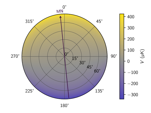
For rapid evaluation of the atmosphere model, a function of the form
| (20) |
can be precisely fit to the simulations, where is the zenith angle and is the azimuth angle, with fit parameters shown in Table 2; zenith angles from were used in the fit. With and specified in , is also in ; is a dimensionless scale factor, and and are angles. The average fit residual is . Parameter , the azimuth offset, corresponds exactly to the magnetic declination. The simulation code used to produce these results has been published (Petroff 2019).
| Parameter | Value |
|---|---|
Note. — When using with equation (20), should be in radians.
IV Comparison with observations
From the CLASS Era 1 survey, nighttime data recorded during the period from 2016 September through 2018 February are used for the present analysis; some nights are excluded due to particularly poor weather conditions or due to operational difficulties, such as interruptions to power or cryogenic systems. For each nightly observation, the telescope was scanned with the boresight center pointing at a zenith angle through an azimuthal range of at a rate of . For the entirety of each night, the boresight rotation angle of the telescope relative to the horizon remained fixed at ; the boresight rotation angle was changed daily such that each angle was observed on a weekly basis. Boresight rotation combined with individual feedhorn pointing offsets provides access to a range of zenith angles from with this scanning strategy.
Of the 28 detector pairs in the Q-band telescope that were operational during the Era 1 survey (Appel et al. 2019), 25 are used for the present analysis, with the remaining three conservatively rejected due to atypical noise properties. Anomalous artifacts found in detector timestreams are excised, along with windows surrounding them chosen such that any filtering operations in the timestream processing pipeline do not convolve the artifacts with surrounding data. The Stokes signal is extracted from pair-differenced detector timestreams via demodulation with the VPM polarization transfer function (Chuss et al. 2012, K. Harrington et al. 2020, in preparation;), where each pair corresponds to the two detectors with orthogonal linear polarization sensitivity in each feedhorn. These resulting timestreams are further checked for stable noise properties, with variance cuts used to eliminate data with abnormally high noise. This data processing pipeline will be described in detail by J. Eimer et al. (2020, in preparation). After all data cuts, 47927.6 detector pair-hours of data remain. Daytime data were excluded from the present analysis, as additional pipeline developments are required to properly handle their reduced stability and artifacts; however, this does not preclude future use of these data. Furthermore, sun avoidance maneuvers alter the telescope’s scan strategy during parts of the day and prevent coverage of the full azimuth range, making these data less suitable for the present analysis.
To confirm that an observed circularly polarized signal is due to atmospheric Zeeman emission, three properties should be satisfied: the azimuth angles of maximum and minimum signal should align with the magnetic declination, the signal should show an appropriate zenith angle dependence, and the signal should have approximately the correct amplitude. To evaluate the observed signal, detector data were divided by detector pair and boresight angle, processed as previously described, binned by azimuth with inverse variance weighting, and fit with a sinusoidal profile; variance was evaluated for timestream segments after splitting the demodulated timestreams into sweeps of constant direction scanning in azimuth. As ground pickup contamination, likely due to leakage, was visible in binned azimuth profiles for some combinations of detector pairs and boresight rotation angles, the azimuth range where the ground elevation angle is above , i.e., where the peak of Cerro Toco is, was masked before fitting; this corresponds to azimuth. A covariance threshold was also used to remove poor fits. As each azimuth sweep is mean-subtracted, only the peak-to-peak amplitude of the azimuth dependent signal is measured, not its absolute offset. Example binned azimuth profiles and sinusoidal fits are shown in Figure 5.
The fits result in a signal maximum aligned with an azimuth angle of , which is consistent with the expected magnetic declination, the angle between magnetic north and true north, of ; this error was calculated using bootstrapping after performing an additional data cut based on the residual after subtracting the sinusoidal best fits from the binned azimuth profiles. The other mechanism by which the Earth’s magnetic field is expected to affect the detector data is through magnetic pickup in the detectors and Superconducting Quantum Interference Device (SQUID) multiplexers and amplifiers. As this pickup is not modulated by the VPM and should therefore not be visible in the demodulated timestreams, this alone is strong evidence of a detection of a signal of atmospheric origin. Next, the zenith angle dependence of the peak-to-peak signal in the data was evaluated and compared to the simulation, the results of which are shown in Figure 6. A data point is shown for each combination of detector pairs and boresight rotation angles; zenith angle differences are due to individual feedhorn pointing offsets, which change relative to the boresight center pointing at different boresight rotation angles. An expected zenith angle dependence is seen, giving further evidence that the observed signal is of atmospheric origin. The excess scatter is thought to be due to uncertainties in the preliminary detector relative efficiency calibrations used in the analysis combined with potential bandpass mismatches between detectors.
As can be seen in Figure 6, the measured amplitude is consistent between different boresight rotation angles and between different detector pairs, providing a check against systematic errors. Additionally, data were split by date of observation to check for changes over time; these splits were also found to be consistent. While there are expected to be slight changes over time to the atmospheric signal due to evolution of the geomagnetic field, these changes are much smaller than the error of the measurements; EMM2017 predicts the yearly change in field strength to be on the sub-percent level and the yearly change in magnetic declination to be approximately .
A ground loop between the VPM control electronics and the detector readout electronics would in theory be able to introduce modulated signal into the SQUID magnetic pickup. However, detector data collected while the VPM was running and the receiver window was covered with a metal plate to block optical signals was inspected and found to contain no modulated signal, ruling out this possibility.
To further exclude the possibility of the detected signal being due to magnetic pickup, the physical geometry of the telescope’s receiver can be considered. The detectors and SQUIDs are all in the same plane relative to one another despite having different optical pointing offsets, i.e., the detectors all have the same physical orientation relative to the magnetic field. Thus, the peak-to-peak amplitude of their magnetic pickup—which should not be in the demodulated timestreams to start with—would only be dependent on the zenith angle of the telescope’s boresight pointing. Since all observations were taken with a boresight pointing zenith angle of , SQUID magnetic pickup would not result in a zenith angle dependence, contrary to the detected signal. Additionally, changing the boresight rotation angle alters the physical orientation of the SQUIDs relative to the magnetic field and thus yields a boresight rotation angle dependence to the magnetic pickup, again contrary to the detected signal.
Using equation (20) and the fit parameters in Table 2, a simulated map was created using pointings from the aforementioned observations, which is shown in Figure 7 along with a map of CLASS data and a map showing residuals. To create the data map, the signal was accumulated into pixels using inverse variance weighting of data, using the same data processing and variance calculation procedures used for fitting the sinusoidal profiles. For the simulated map, azimuth sweeps were mean subtracted and weighted to match the processing of the data. Note that the overall dipole pattern is visible in both maps; the dipole amplitude is in the simulated map and in the data map, with a direction difference of . The dipole amplitude ratio between the simulated map and the data map was used to scale the simulated map before subtracting it from the data map to produce the residual map. If the azimuth sweeps are not mean subtracted when creating the simulated map, the dipole changes in amplitude by and in direction by , demonstrating that the mean subtraction only has a minor effect on the signal. Areas of higher noise are due to uneven sky coverage.

The measured amplitude in both the sinusoidal profiles and map are in reasonable agreement to that predicted by the simulations. The remaining discrepancy is likely due to some combination of calibration errors in the detector data and shortcomings of the simulation. Although the detector calibration was done using Stokes , the demodulated linear polarization of the Crab Nebula matches previous observations (Xu et al. 2019), so it is unlikely that a discrepancy of the magnitude observed between observation and simulation is due to an error in either the VPM polarization transfer function calibration or detector calibration. The detector bandpass uncertainty is also low enough that a bandpass error cannot fully explain the discrepancy (Appel et al. 2019). This leaves a shortcoming of the simulation as the most likely source of the discrepancy. The Van Vleck–Weisskopf line shape is known to be inaccurate far from the resonance lines (Hill 1986), so it may be reasonable to attribute the difference to this inaccuracy, since we are observing at frequencies far from the resonance lines, and the majority of the observed signal is from the lower atmosphere, where the line profile used in the simulations reduces to a Van Vleck–Weisskopf line shape. Furthermore, the line mixing and pressure broadening parameters used in the simulation were also all measured near the resonance lines. As Zeeman splitting of molecular oxygen resonance lines in the presence of Earth’s magnetic field is the only theorized source of circularly polarized atmospheric emission, we conclude that this is the source of the detected signal.
V Conclusion
Expanding on prior models and utilizing recent spectroscopic data, a model for circularly polarized atmospheric emission from Zeeman splitting of molecular oxygen was presented. This model was then used to simulate the atmosphere of the CLASS observing site at the frequencies of the CLASS Q-band telescope. An analysis of circular polarization timestreams observed by the CLASS Q-band telescope, utilizing the Stokes measurement capability of a VPM, was then compared to the simulations and shown to be a strong detection of this atmospheric emission; this is believed to be the first such detection of circular polarization in a frequency band used for ground-based CMB observations. The amplitude of the signal differed by between the simulations and observations but is still in good agreement. As the atmospheric signal is orders of magnitude larger than any theoretical cosmological or astrophysical signal, its subtraction is necessary for setting improved upper limits on said signals and providing more rigorous observational tests. Although this signal can be adequately removed empirically, such as by fitting a dipole sky pattern or by creating templates that describe the signal as a function of azimuth, modeling the signal helps us verify our understanding of it. After the subtraction of the atmospheric signal, Stokes serves primarily as a null channel for CLASS; as no residual signal is expected, a angular power spectrum that is not consistent with zero would suggest the presence of either an unmitigated systematic error or a non-standard cosmological signal.
Acknowledgments
We acknowledge the National Science Foundation Division of Astronomical Sciences for their support of CLASS under Grant Numbers 0959349, 1429236, 1636634, and 1654494. The CLASS project employs detector technology developed in collaboration between JHU and Goddard Space Flight Center under several previous and ongoing NASA grants. Detector development work at JHU was funded by NASA grant number NNX14AB76A. K. Harrington was supported by NASA Space Technology Research Fellowship grant number NX14AM49H. We thank the anonymous reviewer for providing astute comments and suggestions that helped improve this manuscript. We acknowledge scientific and engineering contributions from Max Abitbol, Mario Aguilar, Fletcher Boone, David Carcamo, Francisco Espinoza, Saianeesh Haridas, Connor Henley, Yunyang Li, Lindsay Lowry, Isu Ravi, Gary Rhodes, Daniel Swartz, Bingie Wang, Qinan Wang, Tiffany Wei, and Ziang Yan. We thank María José Amaral, Chantal Boisvert, William Deysher, and Miguel Angel Díaz for logistical support. We acknowledge productive collaboration with Dean Carpenter and the JHU Physical Sciences Machine Shop team. Part of this research project was conducted using computational resources at the Maryland Advanced Research Computing Center (MARCC). We further acknowledge the very generous support of Jim and Heather Murren (JHU A&S ’88), Matthew Polk (JHU A&S Physics BS ’71), David Nicholson, and Michael Bloomberg (JHU Engineering ’64). CLASS is located in the Parque Astronómico Atacama in northern Chile under the auspices of the Comisión Nacional de Investigación Científica y Tecnológica de Chile (CONICYT). R. Dünner and P. Fluxá thank CONICYT for grant BASAL CATA AFB-170002. R. Reeves acknowledges partial support from CATA, BASAL grant AFB-170002, and CONICYT-FONDECYT, through grant 1181620.
References
- Appel et al. (2019) Appel, J. W., Xu, Z., Padilla, I. L., et al. 2019, ApJ, 876, 126, doi: 10.3847/1538-4357/ab1652
- Armstrong (1967) Armstrong, B. 1967, J. Quant. Spec. Radiat. Transf., 7, 61, doi: 10.1016/0022-4073(67)90057-x
- Astropy Collaboration et al. (2013) Astropy Collaboration, Robitaille, T. P., Tollerud, E. J., et al. 2013, A&A, 558, A33, doi: 10.1051/0004-6361/201322068
- Astropy Collaboration et al. (2018) Astropy Collaboration, Price-Whelan, A. M., Sipőcz, B. M., et al. 2018, AJ, 156, 123, doi: 10.3847/1538-3881/aabc4f
- Berestetskii et al. (1982) Berestetskii, V., Lifshitz, E., & Pitaevskii, L. 1982, Quantum Electrodynamics, 2nd edn. (Pergamon Press)
- Born & Wolf (1959) Born, M., & Wolf, E. 1959, Principles of Optics (Pergamon Press)
- Carroll et al. (1990) Carroll, S. M., Field, G. B., & Jackiw, R. 1990, Phys. Rev. D, 41, 1231, doi: 10.1103/PhysRevD.41.1231
- Chulliat et al. (2015) Chulliat, A., Alken, P., Nair, M., Woods, A., & Maus, S. 2015, The Enhanced Magnetic Model 2015–2020, National Centers for Environmental Information, NOAA, doi: 10.7289/v56971hv
- Chuss et al. (2012) Chuss, D. T., Wollack, E. J., Henry, R., et al. 2012, Appl. Opt., 51, 197, doi: 10.1364/ao.51.000197
- Clough et al. (1989) Clough, S., Kneizys, F., & Davies, R. 1989, AtmRe, 23, 229, doi: 10.1016/0169-8095(89)90020-3
- Cooray et al. (2003) Cooray, A., Melchiorri, A., & Silk, J. 2003, PhLB, 554, 1, doi: 10.1016/s0370-2693(02)03291-4
- Eimer et al. (2012) Eimer, J. R., Bennett, C. L., Chuss, D. T., et al. 2012, in Proc. SPIE, ed. W. S. Holland, Vol. 8452 (SPIE), 619–633, doi: 10.1117/12.925464
- Essinger-Hileman et al. (2014) Essinger-Hileman, T., Ali, A., Amiri, M., et al. 2014, in Proc. SPIE, ed. W. S. Holland & J. Zmuidzinas, Vol. 9153 (SPIE), 491–513, doi: 10.1117/12.2056701
- Faddeyeva & Terent′ev (1961) Faddeyeva, V. N., & Terent′ev, N. M. 1961, Mathematical Tables of Values of the Function for Complex Argument, ed. V. A. Fok (Pergamon Press)
- Fixsen (2009) Fixsen, D. J. 2009, ApJ, 707, 916, doi: 10.1088/0004-637X/707/2/916
- Giovannini (2009) Giovannini, M. 2009, Phys. Rev. D, 80, doi: 10.1103/physrevd.80.123013
- Gordon et al. (2017) Gordon, I., Rothman, L., Hill, C., et al. 2017, J. Quant. Spec. Radiat. Transf., 203, 3, doi: 10.1016/j.jqsrt.2017.06.038
- Gorski et al. (2005) Gorski, K. M., Hivon, E., Banday, A. J., et al. 2005, ApJ, 622, 759, doi: 10.1086/427976
- Hanany & Rosenkranz (2003) Hanany, S., & Rosenkranz, P. 2003, New A Rev., 47, 1159, doi: 10.1016/j.newar.2003.09.017
- Harrington et al. (2016) Harrington, K., Marriage, T., Ali, A., et al. 2016, in Proc. SPIE, ed. W. S. Holland & J. Zmuidzinas, Vol. 9914 (SPIE), 380–400, doi: 10.1117/12.2233125
- Harrington et al. (2018) Harrington, K., Ali, A., Appel, J. W., et al. 2018, in Proc. SPIE, ed. J. Zmuidzinas & J.-R. Gao, Vol. 10708 (SPIE), 369–390, doi: 10.1117/12.2313614
- Herbert (1974) Herbert, F. 1974, J. Quant. Spec. Radiat. Transf., 14, 943, doi: 10.1016/0022-4073(74)90021-1
- Hill (1986) Hill, R. J. 1986, RaSc, 21, 447, doi: 10.1029/rs021i003p00447
- Hirsch (2019) Hirsch, M. 2019, space-physics/msise00: MSISE-00 in Python and Matlab, 1.6.1, Zenodo, doi: 10.5281/zenodo.3379163
- Hu & White (1997) Hu, W., & White, M. 1997, New A, 2, 323, doi: 10.1016/s1384-1076(97)00022-5
- Hunter (2007) Hunter, J. D. 2007, CSE, 9, 90, doi: 10.1109/mcse.2007.55
- Inomata & Kamionkowski (2019) Inomata, K., & Kamionkowski, M. 2019, Phys. Rev. D, 99, doi: 10.1103/physrevd.99.043501
- Janssen (1993) Janssen, M. A., ed. 1993, Atmospheric Remote Sensing by Microwave Radiometry (John Wiley & Sons)
- Keating et al. (1998) Keating, B., Timbie, P., Polnarev, A., & Steinberger, J. 1998, ApJ, 495, 580, doi: 10.1086/305312
- King & Lubin (2016) King, S., & Lubin, P. 2016, Phys. Rev. D, 94, doi: 10.1103/physrevd.94.023501
- Koshelev et al. (2015) Koshelev, M. A., Vilkov, I. N., & Tretyakov, M. Y. 2015, J. Quant. Spec. Radiat. Transf., 154, 24, doi: 10.1016/j.jqsrt.2014.11.019
- Koshelev et al. (2016) —. 2016, J. Quant. Spec. Radiat. Transf., 169, 91, doi: 10.1016/j.jqsrt.2015.09.018
- Kunkee et al. (2008) Kunkee, D. B., Poe, G. A., Boucher, D. J., et al. 2008, ITGRS, 46, 863, doi: 10.1109/tgrs.2008.917980
- Kusaka et al. (2018) Kusaka, A., Appel, J., Essinger-Hileman, T., et al. 2018, J. Cosmology Astropart. Phys, 2018, 005, doi: 10.1088/1475-7516/2018/09/005
- Lam et al. (2015) Lam, S. K., Pitrou, A., & Seibert, S. 2015, in LLVM ’15 (ACM Press), doi: 10.1145/2833157.2833162
- Larsson et al. (2014) Larsson, R., Buehler, S. A., Eriksson, P., & Mendrok, J. 2014, J. Quant. Spec. Radiat. Transf., 133, 445, doi: 10.1016/j.jqsrt.2013.09.006
- Larsson et al. (2019) Larsson, R., Lankhaar, B., & Eriksson, P. 2019, J. Quant. Spec. Radiat. Transf., 224, 431, doi: 10.1016/j.jqsrt.2018.12.004
- Lenoir (1967) Lenoir, W. B. 1967, JAP, 38, 5283, doi: 10.1063/1.1709315
- Lenoir (1968) —. 1968, J. Geophys. Res., 73, 361, doi: 10.1029/ja073i001p00361
- Liebe et al. (1993) Liebe, H., Hufford, G., & Cotton, M. 1993, in AGARD Conference Proceedings 542, Atmospheric Propagation Effects Through Natural and Man-Made Obscurants for Visible to MM-Wave Radiation (North Atlantic Treaty Organization). https://apps.dtic.mil/dtic/tr/fulltext/u2/a276919.pdf
- Liebe et al. (1992) Liebe, H., Rosenkranz, P., & Hufford, G. 1992, J. Quant. Spec. Radiat. Transf., 48, 629, doi: 10.1016/0022-4073(92)90127-p
- Liebe (1981) Liebe, H. J. 1981, RaSc, 16, 1183, doi: 10.1029/rs016i006p01183
- Liebe (1989) —. 1989, IJIMW, 10, 631, doi: 10.1007/bf01009565
- Lubin et al. (1983) Lubin, P., Melese, P., & Smoot, G. 1983, ApJ, 273, L51, doi: 10.1086/184128
- Machta & Hughes (1970) Machta, L., & Hughes, E. 1970, Sci, 168, 1582, doi: 10.1126/science.168.3939.1582
- Mainini et al. (2013) Mainini, R., Minelli, D., Gervasi, M., et al. 2013, J. Cosmology Astropart. Phys, 2013, 033, doi: 10.1088/1475-7516/2013/08/033
- Makarov et al. (2011) Makarov, D., Tretyakov, M., & Rosenkranz, P. 2011, J. Quant. Spec. Radiat. Transf., 112, 1420, doi: 10.1016/j.jqsrt.2011.02.018
- Meeks & Lilley (1963) Meeks, M. L., & Lilley, A. E. 1963, J. Geophys. Res., 68, 1683, doi: 10.1029/jz068i006p01683
- Melsheimer et al. (2005) Melsheimer, C., Verdes, C., Buehler, S. A., et al. 2005, RaSc, 40, doi: 10.1029/2004rs003110
- Mohammadi (2014) Mohammadi, R. 2014, EPJC, 74, 3102, doi: 10.1140/epjc/s10052-014-3102-1
- Nagy et al. (2017) Nagy, J. M., Ade, P. A. R., Amiri, M., et al. 2017, ApJ, 844, 151, doi: 10.3847/1538-4357/aa7cfd
- Navas-Guzmán et al. (2015) Navas-Guzmán, F., Kämpfer, N., Murk, A., et al. 2015, AMTD, 8, 1, doi: 10.5194/amtd-8-1-2015
- O’Dea et al. (2007) O’Dea, D., Challinor, A., & Johnson, B. R. 2007, MNRAS, 376, 1767, doi: 10.1111/j.1365-2966.2007.11558.x
- Padilla et al. (2020) Padilla, I. L., Eimer, J. R., Li, Y., et al. 2020, ApJ, 889, 105, doi: 10.3847/1538-4357/ab61f8
- Pardo et al. (1995) Pardo, J., Pagani, L., Gerin, M., & Prigent, C. 1995, J. Quant. Spec. Radiat. Transf., 54, 931, doi: 10.1016/0022-4073(95)00129-9
- Partridge et al. (1988) Partridge, R. B., Nowakowski, J., & Martin, H. M. 1988, Nature, 331, 146, doi: 10.1038/331146a0
- Penndorf (1949) Penndorf, R. 1949, J. Geophys. Res., 54, 7, doi: 10.1029/jz054i001p00007
- Petroff (2019) Petroff, M. A. 2019, Polarized millimeter-wave atmospheric emission model, 1.0, Zenodo, doi: 10.5281/zenodo.3526652
- Picone et al. (2002) Picone, J. M., Hedin, A. E., Drob, D. P., & Aikin, A. C. 2002, JGRA, 107, SIA 15, doi: 10.1029/2002ja009430
- Pietranera et al. (2007) Pietranera, L., Buehler, S. A., Calisse, P. G., et al. 2007, MNRAS, 376, 645, doi: 10.1111/j.1365-2966.2007.11464.x
- Randa et al. (2008) Randa, J., Lahtinen, J., Camps, A., et al. 2008, Recommended Terminology for Microwave Radiometry, Technical Note 1551, NIST, doi: 10.6028/NIST.TN.1551
- Rosenkranz (1998) Rosenkranz, P. W. 1998, RaSc, 33, 919, doi: 10.1029/98rs01182
- Rosenkranz & Staelin (1988) Rosenkranz, P. W., & Staelin, D. H. 1988, RaSc, 23, 721, doi: 10.1029/rs023i005p00721
- Sawyer (2015) Sawyer, R. 2015, Phys. Rev. D, 91, doi: 10.1103/physrevd.91.021301
- Schwartz et al. (2006) Schwartz, M., Read, W., & Snyder, W. V. 2006, ITGRS, 44, 1182, doi: 10.1109/tgrs.2005.862267
- Spinelli et al. (2011) Spinelli, S., Fabbian, G., Tartari, A., Zannoni, M., & Gervasi, M. 2011, MNRAS, 414, 3272, doi: 10.1111/j.1365-2966.2011.18625.x
- Takakura et al. (2019) Takakura, S., Aguilar-Faúndez, M. A. O., Akiba, Y., et al. 2019, ApJ, 870, 102, doi: 10.3847/1538-4357/aaf381
- Tizchang et al. (2016) Tizchang, S., Batebi, S., Haghighat, M., & Mohammadi, R. 2016, EPJC, 76, 478, doi: 10.1140/epjc/s10052-016-4312-5
- Townes & Schawlow (1955) Townes, C. H., & Schawlow, A. L. 1955, Microwave Spectroscopy (McGraw-Hill)
- Tretyakov (2016) Tretyakov, M. 2016, JMoSp, 328, 7, doi: 10.1016/j.jms.2016.06.006
- van der Walt et al. (2011) van der Walt, S., Colbert, S. C., & Varoquaux, G. 2011, CSE, 13, 22, doi: 10.1109/mcse.2011.37
- Van Vleck & Weisskopf (1945) Van Vleck, J. H., & Weisskopf, V. F. 1945, RvMP, 17, 227, doi: 10.1103/revmodphys.17.227
- Varghese & Hanson (1984) Varghese, P. L., & Hanson, R. K. 1984, Appl. Opt., 23, 2376, doi: 10.1364/ao.23.002376
- Virtanen et al. (2019) Virtanen, P., Gommers, R., Oliphant, T. E., et al. 2019, arXiv e-prints. https://arxiv.org/abs/1907.10121
- Watts et al. (2015) Watts, D. J., Larson, D., Marriage, T. A., et al. 2015, ApJ, 814, 103, doi: 10.1088/0004-637X/814/2/103
- Watts et al. (2018) Watts, D. J., Wang, B., Ali, A., et al. 2018, ApJ, 863, 121, doi: 10.3847/1538-4357/aad283
- Xu et al. (2019) Xu, Z., et al. 2019, ApJ, submitted. https://arxiv.org/abs/1911.04499
- Zarei et al. (2010) Zarei, M., Bavarsad, E., Haghighat, M., et al. 2010, Phys. Rev. D, 81, doi: 10.1103/physrevd.81.084035
- Zonca et al. (2019) Zonca, A., Singer, L., Lenz, D., et al. 2019, JOSS, 4, 1298, doi: 10.21105/joss.01298