跳到论文正文
W Papers独立论文阅读器 arXiv:1911.00672 论文正文 计算阅读时间 · 0%
引用这篇论文根据当前论文元数据生成,正式投稿前建议核对。


License: arXiv.org perpetual non-exclusive license
arXiv:1911.00672v3 [math.PR] 05 Oct 2020

Scaling limit for stochastic control problems in population dynamics

Paul Jusselin and Thibaut Mastrolia Note: paul.jusselin@polytechnique.edu Note: thibaut.mastrolia@polytechnique.edu Affiliation: École Polytechnique, CMAP
August 11, 2026
Abstract

Going from a scaling approach for birth/death processes, we investigate the scaling limit of solutions to non-Markovian stochastic control problems by studying the convergence of solutions to BSDEs driven a sequence of converging martingales. In particular we manage to describe how the values and optimal controls of control problems converge when the models converge towards a continuous population model.

Key words: stochastic control, population models, birth and death processes, backward stochastic differential equation (BSDE), stability of BSDEs, martingale properties.

1 Introduction

The sustainability of natural resources has become a major subject of interest in the last decades for public institutions. For instance, in 1983 the European Union has launched its common fisheries policy to manage European fish stocks. In August 2010, a report of European commission named Water Scarcity and Drought in the European Union, has emphasized that ”an adequate supply of good-quality water is a pre-requisite for economic and social progress, so we need to do two things: we must learn to save water, and also to manage our available resources more efficiently”. A large part of academic literature has dealt with such issues. For example, Reed in [Ree79], Clarke and Kirkwood in [CK86], Regnier and De Lara in [RDeL15] or Tromer and Doyen in [TD19] have studied the exploitation of a natural resource under uncertainty on its evolution in a multi-period model. May, Beddington, Horwood and Sherpherd in [MBHS78] have considered the problem by assuming that the intrinsic population growth rate is given by the difference between recruitment and mortality for general recruitment functions. These models have been extended to stochastic differential equations driven by a Brownian motion (see for instance the work of Saphores [Sap03]). Evans, Hening and Shreiber in [EHS15] or more recently Kharroubi, Lim and Ly Vath in [LKLV18] have modelled the dynamic of the natural resource as the solution of the logistic stochastic differential equation to solve a control problem under interaction between species and delayed renewal of the resource. We also refer to the book [DeLD08] for stochastic and deterministic models and resource management problems. All the models mentioned above use a Brownian motion to describe the uncertainty of the system evolution. We refer to this class of model as continuous models. On the other side of the literature, Getz in [Get75] has studied control problems related to a birth/death process. This work has been extended more recently by Claisse in [Cla18] to branching processes. We refer to those models as discrete models.

It is well known that some continuous population models can be seen as scaling limits of discrete models, see for example the work of Bansaye and Méléard in [BM15]. Hence continuous models can be considered as good approximations of the macroscopic evolution of a population size. Therefore it is relevant to consider continuous models for resources management purposes. Moreover those models are attractive from a tractability viewpoint compared to discrete models. Indeed solving control problems in Brownian driven model essentially boils down to solve a partial differential equation. Whereas for discrete models it leads to integral-partial differential equation, which are often more complex to solve. Yet the remaining question is the relevancy of designing a management policy based on a continuous modeling while the controlled population (or resource) is naturally discrete.

To try to give an answer to this question we are going to consider a sequence of discrete population models that converges towards a continuous population model. For each of those models we consider a control problem. Each of them are the natural adaptations of the same control problem to the different models. Therefore we expect the solutions of the discrete control problems to converge towards the solution of the continuous limit problem. From Γ\Gamma-convergence results adapted to stochastic control problems as in for instance the articles of Buttazzo and Del Maso [BDM82] and Belloni, Buttazzo and Freddi [BBF93], we expect to have convergence of value functions (see also for instance [DM12, Theorem 10.22]) and a kind of weak convergence of optimal controls (see for instance [BBF93, Proposition 2.8]). This is emphasized in a toy model (see Section 2) where besides convergence of the value functions we also get convergence in law of the state process under the optimal control. In this paper we prove the convergence of the controls as sequence of processes. This is stronger than Γ−\Gamma-convergence. Since we aim at dealing with non-Markovian stochastic control problems our problematic is to prove the convergence of solutions to a sequence of Backward Stochastic Differential Equations (BSDE for short) driven by a sequence of converging martingales.

We know from the seminal paper of Donsker [Don51] that a scaling in time procedure leads to the weak convergence of a random walk to a Brownian motion. Following the idea of Donsker, Pardoux in [Par99b, Par99a] has studied the weak convergence of Markovian BSDE driven by Brownian motions. Extending this result to the theory of non-Markovian BSDE with fixed time horizon T>0T>0, Briand, Delyon and Mémin in [BDM01] have provided a time discretization of the Brownian motion to get the convergence of a time discretized BSDE. More precisely, they consider a sequence of random walks (Wn)n≥0(W^{n})_{n\geq 0} converging towards a Brownian motion WW. Then they prove the convergence of the solutions of a sequence of BSDEs driven the (Wn)n≥0(W^{n})_{n\geq 0} towards the solution of a BSDE driven by WW. The main idea is to prove the convergence of the terms involved in the martingale representation with respect to WnW^{n} when nn goes to infinity. For this they use the convergence, in the sense of Coquet, Mémin and Slominski [CMS01], of the filtrations associated to each of the (Wn)n≥0(W^{n})_{n\geq 0} towards the natural filtration associated to WW. Those results have been extended in [BDM02] to a more general situation, without assuming that WnW^{n} has a predictable representation property, but assuming that the brackets of the martingales (Wn)n≥0(W^{n})_{n\geq 0} are uniformly bounded. In a more general case, preliminary results on the convergence of BSDEs driven by general martingales have been obtained in the PhD thesis of Alexandros Saplaouras, in L2L^{2} for the Skorokhod distance, see [Sap17, Chapter IV].

In the present paper we aim at extending both the results of [Par99b, BDM01] to a wider class of martingale convergence and the results of [Sap17] to stronger convergence. Starting from a scaling result in [BM15] showing that a sequence of scaled birth/death processes (XK)K≥0(X^{K})_{K\geq 0} with scaling parameter K>0K>0 converges in law to the solution XX of a stochastic Feller diffusion, we begin to extend it to more general birth and death intensities. We then consider a sequence of BSDEs of the form

(𝐁)K:YtK=ξK+∫tTgK​(XsK,YsK,ZsK)⋅ϕsK​d​AsK−∫tTZsK⋅d​MsK,\mathbf{(B)}_{K}:\penalty\ Y^{K}_{t}=\xi^{K}+\int_{t}^{T}g^{K}(X^{K}_{s},Y_{s}^{K},Z^{K}_{s})\cdot\phi^{K}_{s}\mathrm{d}A^{K}_{s}-\int_{t}^{T}Z^{K}_{s}\cdot\mathrm{d}M^{K}_{s},

where ξK\xi^{K} is some general terminal random condition, gKg^{K} the generator of the BSDE, MKM^{K} a two dimensional martingale associated to the population model XKX^{K} and ϕK​d​AK\phi^{K}\mathrm{d}A^{K} denotes the measure associated to the angle bracket of MKM^{K}. We also consider the continuous counterpart of (B)K(\textbf{B})_{K},

(𝐁):Yt=ξ+∫tTg⁡(Xs,Ys,Zs)​d​As−∫tTZs​d​MsX,(\mathbf{B}):\penalty\ Y_{t}=\xi+\int_{t}^{T}g(X_{s},Y_{s},Z_{s})\mathrm{d}A_{s}-\int_{t}^{T}Z_{s}\mathrm{d}M^{X}_{s},

where ξ\xi is some terminal condition, gg is the generator of the BSDE, MXM^{X} is a one dimensional martingale related to the diffusion term of XX and AA is its angle bracket. The existence and uniqueness of solutions to such BSDEs driven by general martingales have been studied, for instance, by El Karoui and Huang in [EKH97], Confortola and Fuhrman in [CF13] or more recently by Papapantoleon, Possamaï and Saplaouras in [PPS18] in a general framework. Inspired by [BDM02], we prove that when (ξK)K≥0(\xi^{K})_{K\geq 0} converges toward ξ\xi and (gK)K≥0(g^{K})_{K\geq 0} towards gg, the solution of (𝐁)K(\mathbf{B})_{K} converges to the solution of (𝐁)(\mathbf{B}). Moreover, since we are motivated by applying our results to stochastic control problems, we prove a stronger convergence, compared to [Sap17], for the solutions to the particular BSDEs considered. To obtain such stronger convergence, we however need to set stronger assumptions on the integrability of terminal conditions (ξK)K≥0(\xi^{K})_{K\geq 0}. The methods used are related to the so-called martingale problem as stated by Jacod and Shiryaev in [JS13] and to the double-Picard iterations craftly used in [BDM02]. Our results enable us to investigate the scaling limit of solutions to non-Markovian stochastic control problems applied to population monitoring.

Main Contributions.

Our approach extends the results in [Par99a, Par99b, BDM01, BDM02] to counting processes, beyond the convergence of a time discretization of the BSDE. This paper is also more focused on applications to stochastic control problems, dealing with examples in population monitoring. We prove that a sequence of solutions to BSDEs driven by birth/death processes converges to a BSDE driven by a one dimensional Brownian motion in tractable spaces to investigate the scaling limits of solutions to stochastic control problems. This also extends the preliminary results on the robustness of solutions to BSDEs in [Sap17, Chapter IV] to the convergence of solutions to our particular BSDE in different spaces. Moreover, the results obtained on the convergence of optimal controls in stochastic control problems go beyond Γ−\Gamma-convergence since we get a strong form of convergence for the optimal controls.

The structure of the paper is the following. In Section 2 we study the convergence of a rescaled birth/death process to the solution of a stochastic Feller type SDE by extending [BM15] to more general dynamics (see Theorem 1). We also provide fundamental properties of our state processes such as exponential moments (see Proposition 1 and Corollary 1). Section 3 introduces a toy model motivating our study and illustrated with numerical simulations. In Section 4, Theorem 2 gives convergence of the solutions to (𝐁)K(\mathbf{B})_{K} to the solution of (𝐁)(\mathbf{B}). In Section 5 from our BSDE approach we deduce convergence of the values and optimal controls to a sequence of control problems. Section 6 gives the main proofs of our results. Minor proofs are given in the appendix.

The spaces considered are defined in Appendix A.

2 From a discrete to a continuous population model

In this section we define a sequence of discrete population models. We show that this sequence converges in law towards a continuous Feller population model by extending [BM15, Theorem III-3.2] to more general population dynamic models.

2.1 Definition of the discrete population models

We consider positive continuous functions fbf^{b}, fdf^{d} and σ\sigma defined from ℝ\mathbb{R} into ℝ+\mathbb{R}^{+} that satisfy the following standing assumption.

Assumption 1.

  • (i)

    The functions fbf^{b}, fdf^{d} and σ\sigma are null on ℝ−\mathbb{R}^{-} and there exists non negative constants ν\nu, μ\mu, η\eta and η¯\underline{\eta} such that for any x∈ℝ+x\in\mathbb{R}^{+}

    fb​(x)≤ν​x,fd​(x)≤μ​x,η¯​x≤σ2​(x)≤η⁡(1+x),f^{b}(x)\leq\nu x,\penalty\ f^{d}(x)\leq\mu x,\penalty\ \underline{\eta}x\leq\sigma^{2}(x)\leq\eta(1+x),
  • (ii)

    f:=fb−fdf:=f^{b}-f^{d} and σ2\sigma^{2} are Lipschitz continuous.

We note Ωd\Omega_{d} the set of piecewise continuous increasing positive functions with jumps equal to 11. We denote by 𝔽\mathbb{F} the natural filtration associated to the canonical process (Nb,Nd)(N^{b},N^{d}) of Ωd2\Omega_{d}^{2}.

For a fixed K≥0K\geq 0 and n≥0n\geq 0 we define a population model on the stochastic basis (Ωd2,𝔽)(\Omega_{d}^{2},\mathbb{F}). The initial population is K​nKn and the processes NbN^{b} and NdN^{d} represent respectively the number of birth and death in the population. This means that when the process NbN^{b} jumps there is a new individual in the population and when NdN^{d} jumps there is one individual less in the population. Therefore at time tt the population size is K​n+Ntb−NtdKn+N_{t}^{b}-N_{t}^{d}. As we are interested in the large population limit (which corresponds to KK large) we consider the rescaled population process

XK,n=n+Nb−NdK.X^{K,n}=n+\frac{N^{b}-N^{d}}{K}.

We define the birth intensity in the model with parameter KK and initial population nn as

λtK,n,b=λK,b​(Xt−K,n):=fb​(Xt−K,n)​K+σ2​(Xt−K,n)2​K2\lambda^{K,n,b}_{t}=\lambda^{K,b}(X^{K,n}_{t-}):=f^{b}(X^{K,n}_{t-})K+\frac{\sigma^{2}(X^{K,n}_{t-})}{2}K^{2}

and the intensity of death

λtK,n,d=λK,d​(Xt−K,n):=fd​(Xt−K,n)​K+σ2​(Xt−K,n)2​K2.\lambda^{K,n,d}_{t}=\lambda^{K,d}(X^{K,n}_{t-}):=f^{d}(X^{K,n}_{t-})K+\frac{\sigma^{2}(X^{K,n}_{t-})}{2}K^{2}.
Remark 1.

Note that fb​(x)=μ​xf^{b}(x)=\mu x, fd​(x)=ν​xf^{d}(x)=\nu x and σ2​(x)=σ2​x\sigma^{2}(x)=\sigma^{2}x satisfy Assumption 1. Consequently, the model studied in Theorem III-3.2 in [BM15] is included in the scope of this paper.

Following Theorem 3.6 in [Jac75] there exists a unique probability measure ℙK,n\mathbb{P}^{K,n} on (Ωd2,𝔽)(\Omega_{d}^{2},\mathbb{F}) such that the processes

MtK,n,i=Nti−∫0tλsK,n,i​𝑑s, for ​i∈{b,d}M^{K,n,i}_{t}=N^{i}_{t}-\int_{0}^{t}\lambda^{K,n,i}_{s}\mathrm{d}s,\text{ for }i\in\{b,d\}

are local martingales. It means that under the probability ℙK,n\mathbb{P}^{K,n} the process NbN^{b} (resp. NdN^{d}) has intensity λK,n,b\lambda^{K,n,b} (resp. λK,n,d\lambda^{K,n,d}). Note that if m>n≥0m>n\geq 0 then ℙK,n\mathbb{P}^{K,n} is absolutely continuous with respect to ℙK,m\mathbb{P}^{K,m} and we have:

d​ℙK,nd​ℙK,m=LTn,m\frac{\mathrm{d}\mathbb{P}^{K,n}}{\mathrm{d}\mathbb{P}^{K,m}}=L^{n,m}_{T} (1)

where

d​Ltn,m=Lt−n,m​(∑i∈{b,d}λtK,n,i−λtK,m,iλtK,m,i​𝟏Xt−K,m>0​d​MtK,m,i)​ with ​L0n,m=1.\mathrm{d}L^{n,m}_{t}=L^{n,m}_{t-}\big(\sum_{i\in\{b,d\}}\frac{\lambda^{K,n,i}_{t}-\lambda^{K,m,i}_{t}}{\lambda^{K,m,i}_{t}}\mathbf{1}_{X^{K,m}_{t-}>0}\mathrm{d}M^{K,m,i}_{t}\big)\text{ with }L^{n,m}_{0}=1.

We justify this change of measure in Appendix B.

For the rest of this work we fix an initial population x0x_{0} and do not write anymore the superscript x0x_{0} to lighten the notations. We write 𝔼\mathbb{E} instead of 𝔼ℙK\mathbb{E}^{\mathbb{P}^{K}} when there is no ambiguity on the probability used. For any KK we consider the processes MK=(MK,b,MK,d)M^{K}=(M^{K,b},M^{K,d}), λtK=λtK,b−λtK,d\lambda^{K}_{t}=\lambda^{K,b}_{t}-\lambda^{K,d}_{t} and for i∈{b,d}i\in\{b,d\}

Λ¯tK,i=∫0tλsK,i​K−2​𝑑s,N¯K,i=Ni​K−2​ and ​M¯K,i=MK,i​K−1.\overline{\Lambda}^{K,i}_{t}=\int_{0}^{t}\lambda^{K,i}_{s}K^{-2}\mathrm{d}s,\penalty\ \overline{N}^{K,i}=N^{i}K^{-2}\text{ and }\overline{M}^{K,i}=M^{K,i}K^{-1}.

We note M¯K=(M¯K,b,M¯K,d)\overline{M}^{K}=(\overline{M}^{K,b},\overline{M}^{K,d}). The rescaled population process is now noted

XK=x0+Nb−NdK.X^{K}=x_{0}+\frac{N^{b}-N^{d}}{K}.

2.2 Scaling limit of the sequence (XK)K≥0(X^{K})_{K\geq 0}

Intuitively, and having in mind [BM15, Theorem 3.2], a continuous version of the processes (XK)K≥0(X^{K})_{K\geq 0}, denoted by XX, would be an Ito diffusion with drift equal to f⁡(X)f(X) and volatility given by σ2​(X)\sigma^{2}(X). We formalize this intuition in the following result which extends [BM15, Theorem 3.2]. The proof is given in Section 6.1.

Theorem 1.

The sequence (XK,M¯K,N¯K,b,N¯K,d,Λ¯K,b,Λ¯K,d)K≥0\big(X^{K},\overline{M}^{K},\overline{N}^{K,b},\overline{N}^{K,d},\overline{\Lambda}^{K,b},\overline{\Lambda}^{K,d}\big)_{K\geq 0} converges in law for the Skorokhod topology towards (X,M,A,A,A,A)(X,M,A,A,A,A) such that

  • (i)

    there exists a bi-dimensional Brownian motions (Bb,Bd)(B^{b},B^{d}) satisfying

    Mt=∫0tσ⁡(Xs)2​d​(Bsb,Bsd),M_{t}=\int_{0}^{t}\frac{\sigma(X_{s})}{\sqrt{2}}\mathrm{d}(B^{b}_{s},B^{d}_{s}),
  • (ii)

    with B=(Bb+Bd)/2B=(B^{b}+B^{d})/\sqrt{2}, the process XX is the unique strong solution of

    (𝐒):Xt=x0+∫0tf⁡(Xs)​𝑑s+σ⁡(Xs)​d​Bs,(\mathbf{S}):\penalty\ X_{t}=x_{0}+\int_{0}^{t}f(X_{s})\mathrm{d}s+\sigma(X_{s})\mathrm{d}B_{s},
  • (iii)

    A=∫0⋅σ2​(Xs)​𝑑sA=\int_{0}^{\cdot}\sigma^{2}(X_{s})\mathrm{d}s.

Moreover, there exists a probability space (Ω,𝔽,ℙ)(\Omega,\mathbb{F},\mathbb{P}) and a sequence (NK,d,NK,b)K≥0(N^{K,d},N^{K,b})_{K\geq 0} such that for any K≥0K\geq 0, (NK,d,NK,b)(N^{K,d},N^{K,b}) has the law of (Nd,Nb)(N^{d},N^{b}) under ℙK\mathbb{P}^{K}. Moreover on this space the sequence

(XK,M¯K,N¯K,b,N¯K,d,Λ¯K,b,Λ¯K,d)K≥0(X^{K},\overline{M}^{K},\overline{N}^{K,b},\overline{N}^{K,d},\overline{\Lambda}^{K,b},\overline{\Lambda}^{K,d})_{K\geq 0}

converges in 𝒮12×𝒮22×𝒮11×𝒮11×𝒮11×𝒮11\mathcal{S}^{2}_{1}\times\mathcal{S}_{2}^{2}\times\mathcal{S}_{1}^{1}\times\mathcal{S}_{1}^{1}\times\mathcal{S}_{1}^{1}\times\mathcal{S}_{1}^{1} to (X,M,A,A,A,A)(X,M,A,A,A,A) when KK goes to +∞+\infty.

According to the last point of Theorem 1 from now on we work under the probability space (Ω,𝔽,ℙ)(\Omega,\mathbb{F},\mathbb{P}) and we consider that the processes (XK,M¯K,N¯K,b,N¯K,d,Λ¯K,b,Λ¯K,d)K≥0(X^{K},\overline{M}^{K},\overline{N}^{K,b},\overline{N}^{K,d},\overline{\Lambda}^{K,b},\overline{\Lambda}^{K,d})_{K\geq 0} and (X,M,A,A,A,A)(X,M,A,A,A,A) are defined on this space. For any KK we note 𝔽K\mathbb{F}^{K} the natural filtration associated to XKX^{K} and 𝔽X\mathbb{F}^{X} the natural filtration associated to XX.

Before going to the next section, we define some processes that we will extensively use in the rest of the paper. We note for i∈{b,d}i\in\{b,d\}

Mti:=∫0tσ⁡(Xs)2​d​Bsi,M^{i}_{t}:=\int_{0}^{t}\frac{\sigma(X_{s})}{\sqrt{2}}\mathrm{d}B^{i}_{s},

so that M=(Md,Mb)M=(M^{d},M^{b}) and MX:=Mb+MdM^{X}:=M^{b}+M^{d} that is written

MtX=∫0tσ⁡(Xs)​d​Bs.M_{t}^{X}=\int_{0}^{t}\sigma(X_{s})\mathrm{d}B_{s}.

We also consider the processes

AtK:=∫0tλsK,b+λsK,dK2​𝑑s,ptK,b:=λtK,bλtK,b+λtK,d, and ​ptK,d:=λtK,dλtK,b+λtK,d.A^{K}_{t}:=\int_{0}^{t}\frac{\lambda^{K,b}_{s}+\lambda^{K,d}_{s}}{K^{2}}\mathrm{d}s,\penalty\ p^{K,b}_{t}:=\frac{\lambda^{K,b}_{t}}{\lambda^{K,b}_{t}+\lambda^{K,d}_{t}},\text{ and }p^{K,d}_{t}:=\frac{\lambda^{K,d}_{t}}{\lambda^{K,b}_{t}+\lambda^{K,d}_{t}}.

Note that under the probability ℙK\mathbb{P}^{K} the random measure mm associated to the process (Nb,Nd)(N^{b},N^{d}) interpreted as a compound jump process with values in E={b,d}E=\{b,d\} admits as predictable compensator measure

πK​(d​e,d​t)=(ϕtK,b​δb​(d​e)+ϕtK,d​δd​(d​e))​d​AtK\pi^{K}(\mathrm{d}e,\mathrm{d}t)=\big(\phi^{K,b}_{t}\delta_{b}(\mathrm{d}e)+\phi^{K,d}_{t}\delta_{d}(\mathrm{d}e)\big)\mathrm{d}A^{K}_{t}

with ϕtK=(ϕtK,b,ϕtK,d)=(ptK,b,ptK,d)​K2\phi^{K}_{t}=(\phi^{K,b}_{t},\phi^{K,d}_{t})=(p^{K,b}_{t},p^{K,d}_{t})K^{2} and where δi\delta_{i} denotes the Dirac measure at point i∈{b,d}i\in\{b,d\}. This point of view is introduced in order to draw a parallel with the framework of [CF13] to which we will refer extensively in Section 4.2.

2.3 Uniform exponential moments

Finally we show that the sequence of processes (XK,∫0⋅XsK)(X^{K},\int_{0}^{\cdot}X_{s}^{K}) admits exponential moments uniformly in KK if σ2\sigma^{2} is linear. The proof of this result is postponed in Appendix F.

Proposition 1.

If there exists a positive constant σ\sigma such that σ2​(x)=σ2​x\sigma^{2}(x)=\sigma^{2}x there exists some positive constants β0\beta_{0}, K0K_{0} and TT such that for any s≤Ts\leq T we have

supK≥K0​𝔼​[exp⁡(β0​∫0sXuK​𝑑u+β0​XsK)]<∞.\underset{K\geq K_{0}}{\sup}\penalty\ \mathbb{E}[{\exp}(\beta_{0}\int_{0}^{s}X^{K}_{u}\mathrm{d}u+\beta_{0}X^{K}_{s})]<\infty.

Without loss of of generality we assume that K0=0K_{0}=0. From now we fix a positive constant β\beta strictly smaller than β0\beta_{0}. As a consequence of Proposition 1, for any integer qq we have for any s≤Ts\leq T

supK≥0​𝔼​[exp⁡(β​∫0sXuK​𝑑u+β​XsK)​(1+|XsK|q)]<+∞\underset{K\geq 0}{\sup}\penalty\ \mathbb{E}[{\exp}(\beta\int_{0}^{s}X^{K}_{u}\mathrm{d}u+\beta X^{K}_{s})(1+|X^{K}_{s}|^{q})]<+\infty

and

supK≥0​𝔼​[∫0Texp⁡(β​∫0sXuK​𝑑u+β​XsK)​(1+|XsK|q)​𝑑s]<+∞.\underset{K\geq 0}{\sup}\penalty\ \mathbb{E}[\int_{0}^{T}{\exp}(\beta\int_{0}^{s}X^{K}_{u}\mathrm{d}u+\beta X^{K}_{s})(1+|X^{K}_{s}|^{q})\mathrm{d}s]<+\infty.

We deduce from Fatou’s Lemma together with Proposition 1 that XX inherits from the exponential moments of XKX^{K} as stated in the following corollary.

Corollary 1.

If there exists σ\sigma positive such that σ2​(x)=σ2​x\sigma^{2}(x)=\sigma^{2}x there exists some positive constants β0\beta_{0} and TT such that for any s≤Ts\leq T we have

𝔼⁡[exp⁡(β0​∫0sXu​𝑑u+β0​Xs)]<∞.\mathbb{E}[{\exp}(\beta_{0}\int_{0}^{s}X_{u}\mathrm{d}u+\beta_{0}X_{s})]<\infty.

In order to benefit from those exponential moments we now assume that σ2​(x)=σ2​x\sigma^{2}(x)=\sigma^{2}x for some positive constant σ\sigma fixed.

3 Illustration of the study on a toy model

In this section, we illustrate the Γ−\Gamma-convergence result applied to optimization problems in population dynamics. We consider specific parameters fd,fbf^{d},\penalty\ f^{b} and a sequence of control problems for which we are able to make explicit computations. Then, we show that the sequence of optimal controls converges in law to the optimal control of a continuous problem. In this section, we aim at providing the general main ideas of the paper rather than being perfectly accurate. Rigorous statements will be given in Section 5.

3.1 Discrete populations models

We consider a discrete birth/death model as studied in [BM15] by choosing:

  • -

    the initial population x0∈ℕx_{0}\in\mathbb{N},

  • -

    the birth rate fb​(x)=ν​xf^{b}(x)=\nu x for some ν>0\nu>0,

  • -

    the death rate fd​(x)=μ​xf^{d}(x)=\mu x for some μ>0\mu>0.

Recall from Remark 1 and from [BM15, Theorem 3.2] that (XtK)t∈[0,T](X_{t}^{K})_{t\in[0,T]} converges in law for the Skorokhod topology towards the continuous diffusion process (Xt)t∈[0,T](X_{t})_{t\in[0,T]} solution of the Feller stochastic differential equation

d​Xt=(ν−μ)​Xt​d​t+σ​Xs​d​Wt,\mathrm{d}X_{t}=(\nu-\mu)X_{t}\mathrm{d}t+\sigma\sqrt{X_{s}}\mathrm{d}W_{t}, (2)

for WW a Brownian motion.

In this toy model, we assume that a resource manager regulates the population XKX^{K} through an 𝔽K\mathbb{F}^{K}-predictable control α\alpha. A control α\alpha is admissible if

  • •

    there exists a unique law ℙK,α\mathbb{P}^{K,\alpha} under which the death intensity of the population is

    λtK,d,α:=K​XtK​(μ+K​σ22)+K​XtK​αt,\lambda_{t}^{K,d,\alpha}:=KX_{t}^{K}(\mu+K\frac{\sigma^{2}}{2})+KX_{t}^{K}\alpha_{t},

    and the birth intensity is λK,b\lambda^{K,b}. When this probability exists, it is the law of the population under the control α\alpha.

  • •

    λK,d,α\lambda^{K,d,\alpha} is a non negative process ℙK,α\mathbb{P}^{K,\alpha} almost surely.

We denote by 𝒜K\mathcal{A}^{K} the set of admissible controls.

The agent is assumed to be penalized if he fails at reaching a fixed level x~>0\widetilde{x}>0 of the resource at time TT determined by a regulator. We model this penalization by the square of the difference between the effective population size at time TT and the target x~\tilde{x}. So that the manager pays γ​(XTK−x~)2\gamma(X_{T}^{K}-\widetilde{x})^{2} at time TT where γ\gamma is a positive constant. The manager payoff is also assumed to be penalized by the instantaneous amount |αt​XtK|22\frac{|\alpha_{t}X_{t}^{K}|^{2}}{2} per unit of time when its effort is α\alpha. The problem of the resource manager is thus to solve

(TM)K:V0K=supα∈𝒜K​𝔼K,α​[−γ​(XTK−x~)2−∫0T(αs​XsK)22​𝑑s](\textbf{TM})_{K}:\penalty\ V_{0}^{K}=\underset{\alpha\in\mathcal{A}^{K}}{\sup}\;\mathbb{E}^{K,\alpha}[-\gamma(X_{T}^{K}-\widetilde{x})^{2}-\int_{0}^{T}\frac{(\alpha_{s}X_{s}^{K})^{2}}{2}\mathrm{d}s]

where 𝔼K,α\mathbb{E}^{K,\alpha} denotes the expectation taken under the probability ℙK,α\mathbb{P}^{K,\alpha}. We assume that σ2>2​γ​x~\sigma^{2}>2\gamma\tilde{x} and γ<μ\gamma<\mu.

To solve this problem, as usual in stochastic control theory, we study the corresponding Hamilton-Jacobi-Bellman (HJB for short) equation and use a verification argument. The HJB equation associated to the control problem (TM)K(\textbf{TM})_{K} is

(HJB)K​{∂tUK(t,x)+HK(x,D+KUK(t,x),D−KUK(t,x))=0,(t,x)∈[0,T)×(ℕ∗/K),UK(T,x)=−γ(x−x~)2,x∈(ℕ∗/K),(\textbf{HJB})_{K}\begin{cases}\partial_{t}U^{K}(t,x)+H^{K}\big(x,D_{+}^{K}U^{K}(t,x),D_{-}^{K}U^{K}(t,x)\big)=0,\quad(t,x)\in[0,T)\times(\mathbb{N}^{*}/K),\\ U^{K}(T,x)=-\gamma(x-\widetilde{x})^{2},\quad x\in(\mathbb{N}^{*}/K),\end{cases}

with Hamiltonian HKH^{K} given by

HK​(x,p+,p−)=supα{K​x​(ν+σ22​K)​p++K​x​(μ+α+σ22​K)​p−−(α​x)22},H^{K}(x,p^{+},p_{-})=\sup_{\alpha}\Big\{Kx(\nu+\frac{\sigma^{2}}{2}K)p_{+}+Kx(\mu+\alpha+\frac{\sigma^{2}}{2}K)p_{-}-\frac{(\alpha x)^{2}}{2}\Big\},

and where

D+K​UK​(t,x)=UK​(t,x+1/K)−UK​(t,x)​ and ​D−K​UK​(t,x)=UK​(t,x−1/K)−UK​(t,x).D^{K}_{+}U^{K}(t,x)=U^{K}(t,x+1/K)-U^{K}(t,x)\text{ and }\penalty\ D^{K}_{-}U^{K}(t,x)=U^{K}(t,x-1/K)-U^{K}(t,x).

The maximizer of the Hamiltonian is αK,∗=K​p−x​𝟏x>0\alpha^{K,*}=\frac{Kp_{-}}{x}\mathbf{1}_{x>0}, hence

HK​(x,p+,p−)=K​x​(ν+σ22​K)​p++K​x​(μ+σ22​K)​p−+(K​p−)22​𝟏x>0.H^{K}(x,p^{+},p_{-})=Kx(\nu+\frac{\sigma^{2}}{2}K)p_{+}+Kx(\mu+\frac{\sigma^{2}}{2}K)p_{-}+\frac{(Kp_{-})^{2}}{2}\mathbf{1}_{x>0}.

Note that we do not actually care about the value of the control when x=0x=0 since if the population reaches 00, it is stuck at this value. The partial differential equation (PDE for short) (HJB)K(\textbf{HJB})_{K} is quadratic, so we search for a solution under the form

UK​(t,x)=aK​(t)​x2+bK​(t)​x+cK​(t).U^{K}(t,x)=a_{K}(t)x^{2}+b_{K}(t)x+c_{K}(t).

Identifying the monomials, we get that UKU^{K} is solution of (𝐇𝐉𝐁)K(\mathbf{HJB})_{K} if and only if (aK,bK,cK)(a_{K},b_{K},c_{K}) is solution of the following systems of ODEs:

(ODE)K:{aK′​(t)+2​aK​(t)​(ν−μ)+2​aK2​(t)=0,aK​(T)=−γ,bK′​(t)−2​aK​(t)​(aK​(t)K−bK​(t))+aK​(t)​(σ2+μ+νK)+bK​(t)​(ν−μ)=0,bK​(T)=2​γ​x~,cK′​(t)+12​(aK​(t)K−bK​(t))2=0,cK​(T)=−γ​x~2.\textbf{(ODE)}_{K}:\penalty\ \left\{\begin{array}[]{ll}a_{K}^{\prime}(t)+2a_{K}(t)(\nu-\mu)+2a_{K}^{2}(t)=0,&\penalty\ a_{K}(T)=-\gamma,\\ b_{K}^{\prime}(t)-2a_{K}(t)\big(\frac{a_{K}(t)}{K}-b_{K}(t)\big)+a_{K}(t)(\sigma^{2}+\frac{\mu+\nu}{K})+b_{K}(t)(\nu-\mu)=0,&\penalty\ b_{K}(T)=2\gamma\widetilde{x},\\ c_{K}^{\prime}(t)+\frac{1}{2}\big(\frac{a_{K}(t)}{K}-b_{K}(t)\big)^{2}=0,&\penalty\ c_{K}(T)=-\gamma\widetilde{x}^{2}.\end{array}\right.

By Cauchy-Lipschitz theorem this system admits a unique solution. Thus the optimal effort of the agent is

αtK,∗=1XtK​(aK​(t)K−2​XtK​aK​(t)−bK​(t))​𝟏XtK>0\alpha^{K,*}_{t}=\frac{1}{X_{t}^{K}}\Big(\frac{a_{K}(t)}{K}-2X_{t}^{K}a_{K}(t)-b_{K}(t)\Big)\mathbf{1}_{X^{K}_{t}>0}

and the corresponding death intensity is given by

λtK,d,αK,∗=K​XtK​(μ+K​σ22)+(−2​XtK​aK​(t)+aK​(t)​XtKK−bK​(t))​𝟏XtK>0.\lambda^{K,d,\alpha^{K,*}}_{t}=KX_{t}^{K}(\mu+K\frac{\sigma^{2}}{2})+\big(-2X_{t}^{K}a_{K}(t)+\frac{a_{K}(t)X^{K}_{t}}{K}-b_{K}(t)\big)\mathbf{1}_{X_{t}^{K}>0}.

Note that in view of (ODE)K(\textbf{ODE})_{K} and since aK​(T)a_{K}(T) is negative and bK​(T)b_{K}(T) positive, there exists a TT small enough, independent of KK, such that for any KK the control αK,∗\alpha^{K,*} is in 𝒜K\mathcal{A}^{K}. We refer to Appendix C for more details on this point. We assume that we are considering such short enough time horizon here.

3.2 Continuous populations model

We now turn to the continuous version of the control problem. We assume that the manager controls the drift term in (2) through an 𝔽X−\mathbb{F}^{X}-predictable process α\alpha. We say that α\alpha is an admissible control when the following SDE admits a unique weak solution

d​Xt=(ν−μ−αt)​Xt​d​t+σ​Xt​d​Wt.\mathrm{d}X_{t}=(\nu-\mu-\alpha_{t})X_{t}\mathrm{d}t+\sigma\sqrt{X_{t}}\mathrm{d}W_{t}.

When such solution exists we note ℙα\mathbb{P}^{\alpha} its law that is the law of the population under the control α\alpha. We denote by 𝒜\mathcal{A} the set of admissible controls.

The control problem in the continuous framework is written

(TM):V0=supα∈𝒜​𝔼α​[−γ​(XT−x~)2−∫0T(αs​Xs)22​𝑑s].(\textbf{TM}):\penalty\ V_{0}=\underset{\alpha\in\mathcal{A}}{\sup}\;\mathbb{E}^{\alpha}[-\gamma(X_{T}-\widetilde{x})^{2}-\int_{0}^{T}\frac{(\alpha_{s}X_{s})^{2}}{2}\mathrm{d}s].

The associated HJB equation is given by

(HJB)​{∂tU(t,x)+H(x,DU(t,x),ΔU(t,x))=0,(t,x)∈[0,T)×ℝ+,U(T,x)=−γ(x−x~)2,x∈ℝ+,(\textbf{HJB})\begin{cases}\partial_{t}U(t,x)+H(x,DU(t,x),\Delta U(t,x))=0,\quad(t,x)\in[0,T)\times\mathbb{R}^{+},\\ U(T,x)=-\gamma(x-\widetilde{x})^{2},\quad x\in\mathbb{R}^{+},\end{cases}

where the Hamiltonian HH is

H⁡(x,p,q)=supα{(ν−μ−α)​x​p−|α​x|22+12​x​σ2​q}=(ν−μ)​x​p+12​x​σ2​q+p22​𝟏x>0.\displaystyle H(x,p,q)=\sup_{\alpha}\Big\{(\nu-\mu-\alpha)xp-\frac{|\alpha x|^{2}}{2}+\frac{1}{2}x\sigma^{2}q\Big\}=(\nu-\mu)xp+\frac{1}{2}x\sigma^{2}q+\frac{p^{2}}{2}\mathbf{1}_{x>0}.

The maximizer of the Hamiltonian is

α∗​(x,p)=−px​𝟏x>0\alpha^{*}(x,p)=\frac{-p}{x}\mathbf{1}_{x>0}

As previously, we are looking for a quadratic solution of the form

U⁡(t,x)=a⁡(t)​x2+b⁡(t)​x+c⁡(t).U(t,x)=a(t)x^{2}+b(t)x+c(t).

Identifying the monomials, we get that UU is solution of (HJB)(\textbf{HJB}) if and only if (a,b,c)(a,b,c) is solution of the following system of ODEs.

(ODE):{a′​(t)+2​a​(t)​(ν−μ)+2​a2​(t)=0,a⁡(T)=−γ,b′​(t)+2​a​(t)​b​(t)+a⁡(t)​σ2+b⁡(t)​(ν−μ)=0,b⁡(T)=2​γ​x~,c′​(t)+|b⁡(t)|22=0,c⁡(T)=−γ​x~2.\textbf{(ODE)}:\penalty\ \left\{\begin{array}[]{ll}a^{\prime}(t)+2a(t)(\nu-\mu)+2a^{2}(t)=0,&\penalty\ a(T)=-\gamma,\\ b^{\prime}(t)+2a(t)b(t)+a(t)\sigma^{2}+b(t)(\nu-\mu)=0,&\penalty\ b(T)=2\gamma\widetilde{x},\\ c^{\prime}(t)+\frac{|b(t)|^{2}}{2}=0,&\penalty\ c(T)=-\gamma\widetilde{x}^{2}.\end{array}\right.

Hence, the optimal control is given by

αt∗=−D​U​(t,Xt)Xt​𝟏Xt>0=−2​a​(t)​Xt+b⁡(t)Xt​𝟏Xt>0.\alpha^{*}_{t}=-\frac{DU(t,X_{t})}{X_{t}}\mathbf{1}_{X_{t}>0}=-\frac{2a(t)X_{t}+b(t)}{X_{t}}\mathbf{1}_{X_{t}>0}.

Note that in view of (ODE)(\textbf{ODE}) and since a⁡(T)a(T) is negative and b⁡(T)b(T) positive, there exists a TT small enough such that the control α∗\alpha^{*} is in 𝒜\mathcal{A}, see Appendix C for details. We assume that we are considering such time horizon here. We also note that aK=aa_{K}=a and as consequence of Grönwall Lemma (bK,cK)K≥0(b_{K},c_{K})_{K\geq 0} converges to (b,c)(b,c) when KK goes to +∞+\infty. Consequently we get the convergence of the value of the control problems, limK→+∞V0K=V0\lim\limits_{K\to+\infty}V_{0}^{K}=V_{0}. Moreover a direct adaption of the proof of Proposition 1 gives the convergence in law of the optimally controlled population:

limK→+∞ℙK,αK,∗=ℙα∗.\lim\limits_{K\to+\infty}\mathbb{P}^{K,\alpha^{K,*}}=\mathbb{P}^{\alpha^{*}}.

Those convergences are illustrated in Figures 1 and 2 respectively.
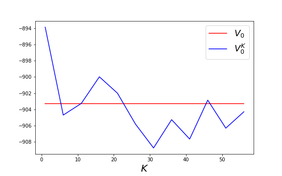
Refer to caption
Figure 1: Convergence of (V0K)K≥0(V_{0}^{K})_{K\geq 0} towards V0V_{0} with σ2=0.3\sigma^{2}=0.3, μ=0.1\mu=0.1, ν=0.2\nu=0.2, T=0.1T=0.1, x0=50x_{0}=50, x~=20\tilde{x}=20 and γ=1\gamma=1.
Refer to caption
Figure 2: Empirical distribution of the discrete optimal controls at time t=0.1t=0.1 for different values of KK (in red) compared to the distribution of the continuous optimal control. The parameters are the same than in Figure 1

.

4 Convergence of BSDEs

In this section we prove the main results of this paper. We recall a convergence result of a sequence of martingale representations given in [PPS19]. Then we extend it to the convergence of a sequence of BSDEs driven by the sequence of martingales (MK)K≥0(M^{K})_{K\geq 0}.

4.1 Convergence of martingale representations

From Theorem 2 in [Dav76] we know any 𝔽K−\mathbb{F}^{K}-martingale has the representation property with respect to MKM^{K} (in the sense of Definition III-4.22 in [JS13]). Moreover we prove in Appendix E that any 𝔽X−\mathbb{F}^{X}- martingale has the representation property relative to MXM^{X}.

For any K≥0K\geq 0 we consider ξK∈L2\xi^{K}\in L^{2} an ℱTK\mathcal{F}_{T}^{K}-measurable real random variable and ξ∈L2\xi\in L^{2} an ℱTX\mathcal{F}_{T}^{X}-measurable real random variable. We define the closed martingale QKQ^{K} by QtK=𝔼⁡[ξK|ℱtK]Q^{K}_{t}=\mathbb{E}[\xi^{K}|\mathcal{F}^{K}_{t}], ℙ−\mathbb{P}-a.s.. Since QKQ^{K} is an 𝔽K\mathbb{F}^{K}-martingale and ξK∈L2\xi^{K}\in L^{2}, we know that there exists a unique process ZK∈L2​(MK)Z^{K}\in L^{2}(M^{K}) such that

QtK=𝔼⁡[ξK|ℱtK]=Q0K+∫0tZsK⋅d​MsK.Q^{K}_{t}=\mathbb{E}[\xi^{K}|\mathcal{F}^{K}_{t}]=Q^{K}_{0}+\int_{0}^{t}Z^{K}_{s}\cdot\mathrm{d}M^{K}_{s}.

Similarly considering the 𝔽X\mathbb{F}^{X}-martingale QQ defined by Qt=𝔼⁡[ξ|ℱt]Q_{t}=\mathbb{E}[\xi|\mathcal{F}_{t}], ℙ−a.s.\mathbb{P}-a.s. since ξ∈𝕃2\xi\in\mathbb{L}^{2} we have existence and uniqueness of Z∈L2​(MX)Z\in L^{2}(M^{X}) such that

Qt=𝔼⁡[ξ|ℱtX]=Q0+∫0tZs​d​MsX.Q_{t}=\mathbb{E}[\xi|\mathcal{F}^{X}_{t}]=Q_{0}+\int_{0}^{t}Z_{s}\mathrm{d}M^{X}_{s}.

We have the following result as a mere extension of [PPS19, Theorem 3.3].

Proposition 2 (martingale representations convergence).

If the sequence (ξK)K≥0(\xi^{K})_{K\geq 0} and ξ\xi are in L2+εL^{2+\varepsilon} and (ξK)K≥0(\xi^{K})_{K\geq 0} converges towards ξ\xi in L2+εL^{2+\varepsilon} for ε>0\varepsilon>0 then

(QK,⟨QK,QK⟩,⟨QK,M¯K⟩)→(Q,⟨Q,Q⟩,⟨Q,M⟩)​ as ​K→+∞\Big(Q^{K},\langle Q^{K},Q^{K}\rangle,\langle Q^{K},\overline{M}^{K}\rangle\Big)\rightarrow\Big(Q,\langle Q,Q\rangle,\langle Q,M\rangle\Big)\text{ as }K\rightarrow+\infty

in 𝒮12+ε′×𝒮11+ε′/2×𝒮22+ε′\mathcal{S}^{2+\varepsilon^{\prime}}_{1}\times\mathcal{S}^{1+\varepsilon^{\prime}/2}_{1}\times\mathcal{S}^{2+\varepsilon^{\prime}}_{2} for any ε′∈[0,ε)\varepsilon^{\prime}\in[0,\varepsilon).

Compared to Theorem 5 in [BDM02] or Theorem 3.3 [PPS19] we have assumed that the convergence of (ξK)K≥0(\xi^{K})_{K\geq 0} takes place in L2+εL^{2+\varepsilon} instead in L2L^{2}. This is in order to extend the convergence of (⟨QK,M¯K⟩)K≥0(\langle Q^{K},\overline{M}^{K}\rangle)_{K\geq 0} beyond 𝒮21\mathcal{S}^{1}_{2}. Indeed if we only assume that ⟨QK⟩∈𝒮11\langle Q^{K}\rangle\in\mathcal{S}^{1}_{1}, ⟨QK,M¯K⟩\langle Q^{K},\overline{M}^{K}\rangle is not squared integrable a priori. In [BDM02] the authors do not face this issue since they assume that the brackets of the martingales they consider are bounded, see Hypothesis (H​1)(H1). In our framework the sequence (⟨M¯K⟩T)K≥0(\langle\overline{M}^{K}\rangle_{T})_{K\geq 0} is not bounded in general. However, if we instead consider a sequence of models with a bounded population then (⟨M¯K⟩T)K≥0(\langle\overline{M}^{K}\rangle_{T})_{K\geq 0} would be bounded and we could get the same result assuming only the convergence of (ξK)K≥0(\xi^{K})_{K\geq 0} in L2L^{2} only.

4.2 Convergence of BSDEs

We now extend the previous result to convergence of a sequence of BSDEs driven by MKM^{K}.

For any K≥0K\geq 0 we consider an ℱTK\mathcal{F}^{K}_{T} random variable ξK\xi^{K} and two continuous functions gbKg^{K}_{b} and gdKg^{K}_{d} from ℝ3\mathbb{R}^{3} into ℝ\mathbb{R}. We write for (x,y,z)∈ℝ×ℝ×ℝ2(x,y,z)\in\mathbb{R}\times\mathbb{R}\times\mathbb{R}^{2}

gK​(x,y,z)=(gbK​(x,y,zb),gdK​(x,y,zd)).g^{K}(x,y,z)=\big(g_{b}^{K}(x,y,z^{b}),g_{d}^{K}(x,y,z^{d})\big).

Note that in the above equation, we implicitly use the decomposition z=(zb,zd)z=(z^{b},z^{d}). We will always assume such convention when we are dealing with a pair of elements such that one element of the pair is related to the birth in the population and the other is related to the death.

We introduce the BSDE with generator gKg^{K} and terminal value ξK\xi^{K} by setting

(𝐁)K:YtK=ξK+∫tTgK​(XsK,YsK,ZsK)⋅ϕsK​d​AsK−∫tTZsK⋅d​MsK.(\mathbf{B})_{K}:\penalty\ Y^{K}_{t}=\xi^{K}+\int_{t}^{T}g^{K}(X^{K}_{s},Y^{K}_{s},Z^{K}_{s})\cdot\phi^{K}_{s}\mathrm{d}A^{K}_{s}-\int_{t}^{T}Z^{K}_{s}\cdot\mathrm{d}M^{K}_{s}.
Definition 1.

A solution to BSDE (𝐁)K(\mathbf{B})_{K} is a pair of processes (Y,Z)∈𝕊K(Y,Z)\in\mathbb{S}^{K} such that the relation (𝐁)K(\mathbf{B})_{K} holds ℙ−a.s.\mathbb{P}-a.s.

As a consequence of Theorem 3.4 in [CF13] we have the following result.

Lemma 1.

Assume that

  • (i)

    ξK∈𝕋K\xi^{K}\in\mathbb{T}^{K},

  • (ii)

    there exists a positive constant LL such that β>L2+2​L\beta>L^{2}+2L and for any x,y,y′,z,z′x,y,y^{\prime},z,z^{\prime} and K≥0K\geq 0 we have for j∈{b,d}j\in\{b,d\}

    K2​|gjK​(x,y,z/K)−gjK​(x,y′,z′/K)|≤L⁡(|y−y′|+|z−z′|),K^{2}|g_{j}^{K}(x,y,z/K)-g_{j}^{K}(x,y^{\prime},z^{\prime}/K)|\leq L\big(|y-y^{\prime}|+|z-z^{\prime}|\big),
  • (iii)

    gj​(XtK,0,0)∈ℍ1Kg_{j}(X^{K}_{t},0,0)\in\mathbb{H}_{1}^{K} for j∈{b,d}j\in\{b,d\},

then the BSDE (𝐁)K(\mathbf{B})_{K} has a unique solution (YK,ZK)∈𝕊K(Y^{K},Z^{K})\in\mathbb{S}^{K}.

We also introduce a class of BSDE driven by the martingale MXM^{X}. For an ℱTX\mathcal{F}^{X}_{T} real valued random variable ξ\xi and a continuous function gg from ℝ3\mathbb{R}^{3} into ℝ\mathbb{R} we consider the BSDE

(𝐁):Yt=ξ+∫tTg⁡(Xs,Ys,Zs)​d​As−∫tTZs​d​MsX.(\mathbf{B}):\penalty\ Y_{t}=\xi+\int_{t}^{T}g(X_{s},Y_{s},Z_{s})\mathrm{d}A_{s}-\int_{t}^{T}Z_{s}\mathrm{d}M^{X}_{s}.
Definition 2.

A solution to BSDE (𝐁)(\mathbf{B}) is a pair of processes (Y,Z)∈𝕊(Y,Z)\in\mathbb{S} such that the relation (𝐁)(\mathbf{B}) holds ℙ−a.s.\mathbb{P}-a.s.

We get the following result on existence and uniqueness of solution to (𝐁)(\mathbf{B}) which is a consequence of Theorem 6.1 in [EKH97] or Theorem 2.1 in [CFS08].

Lemma 2.

Assume that

  • (i)

    ξ∈𝕋\xi\in\mathbb{T},

  • (ii)

    there exists a positive constant LL such that β>L2+2​L\beta>L^{2}+2L and for any x,y,y′,z,z′x,y,y^{\prime},z,z^{\prime} we have:

    |g⁡(x,y,z)−g⁡(x,y′,z′)|≤L⁡(|y−y′|+|z−z′|),|g(x,y,z)-g(x,y^{\prime},z^{\prime})|\leq L\big(|y-y^{\prime}|+|z-z^{\prime}|\big),
  • (iii)

    g⁡(Xt,0,0)∈ℍg(X_{t},0,0)\in\mathbb{H},

then the BSDE (𝐁)(\mathbf{B}) has a unique solution (Y,Z)∈𝕊(Y,Z)\in\mathbb{S}.

We are interested in the convergence of the solutions to (𝐁)K(\mathbf{B})_{K} when (ξK)K≥K(\xi^{K})_{K\geq K} and (gK)K≥0(g^{K})_{K\geq 0} converge. Therefore we make the following converging assumptions on the drivers of the BSDEs (𝐁)K(\mathbf{B})_{K}.

Assumption 2.

  • (i)

    The sequence (ξK)K≥0(\xi^{K})_{K\geq 0} converges towards ξ∈𝕋\xi\in\mathbb{T} in L2+εL^{2+\varepsilon} for ε>0\varepsilon>0,

  • (ii)

    there exists a positive constant CC such that for any x,x′,y,zx,x^{\prime},y,z, K≥0K\geq 0 and j∈{b,d}j\in\{b,d\}

    K2​|gjK​(x,y,z)−gjK​(x′,y,z)|≤C​|x−x′|,K^{2}|g_{j}^{K}(x,y,z)-g_{j}^{K}(x^{\prime},y,z)|\leq C|x-x^{\prime}|,
  • (iii)

    there exists a pair of continuous functions (gb,gd)(g_{b},g_{d}) from ℝ3\mathbb{R}^{3} and a positive sequence (υK)K≥0(\upsilon_{K})_{K\geq 0} converging towards 00 such that for any K≥0K\geq 0, x,yx,y and zz we have for j∈{b,d}j\in\{b,d\}:

    |K2​gjK​(x,y,z/K)−gj​(x,y,z)|≤υK​(1+x2+y2+‖z‖2).|K^{2}g_{j}^{K}(x,y,z/K)-g_{j}(x,y,z)|\leq\upsilon_{K}(1+x^{2}+y^{2}+\|z\|^{2}).
Remark 2.

Under Assumption 2 (iii) if for any KK the pair (gbK,gdK)(g_{b}^{K},g^{K}_{d}) satisfies assumptions (ii) and (iii) in Lemma 1 then the function g=(gb+gd)/2g=(g_{b}+g_{d})/2 satisfies the assumptions (ii) and (iii) in Lemma 2.

For any K≥0K\geq 0 we consider (YK,ZK)∈𝕊K(Y^{K},Z^{K})\in\mathbb{S}^{K} the unique solution of (𝐁)K(\mathbf{B})_{K}. We have the following convergence result for the sequence (YK,ZK)K≥0(Y^{K},Z^{K})_{K\geq 0} whose proof is given in Section 6.2.

Theorem 2.

Under Assumption 2 if the assumptions of Lemma 1 are satisfied for any KK then the BSDE driven by MXM^{X} with generator g:=gb+gd2g:=\frac{g_{b}+g_{d}}{2} and terminal value ξ\xi has a unique solution (Y,Z)(Y,Z) and we have the following convergence:

(YK,∫0⋅ZtK⋅d​MtK,⟨YK,M¯K⟩,⟨YK⟩)→(Y,∫0⋅Zt​d​MtX,⟨Y,M⟩,⟨Y⟩)​ as ​K→+∞\Big(Y^{K},\int_{0}^{\cdot}Z^{K}_{t}\cdot\mathrm{d}M^{K}_{t},\langle Y^{K},\overline{M}^{K}\rangle,\langle Y^{K}\rangle\Big)\rightarrow\Big(Y,\int_{0}^{\cdot}Z_{t}\mathrm{d}M_{t}^{X},\langle Y,M\rangle,\langle Y\rangle\Big)\text{ as }K\rightarrow+\infty

in 𝒮12×𝒮12×𝒮21×𝒮11\mathcal{S}^{2}_{1}\times\mathcal{S}^{2}_{1}\times\mathcal{S}^{1}_{2}\times\mathcal{S}^{1}_{1}.

The convergence in Theorem 2 implies the following convergence

(∫0⋅ZtK,bK​λtK,b​𝑑t,∫0⋅ZtK,dK​λtK,d​𝑑t,∫0⋅|ZtK|2⋅ϕtK​d​AtK)→(∫0⋅Zt​d​At/2,∫0⋅Zt​d​At/2,∫0⋅Zt2​d​At),\displaystyle\Big(\int_{0}^{\cdot}\frac{Z^{K,b}_{t}}{K}\lambda^{K,b}_{t}\mathrm{d}t,\int_{0}^{\cdot}\frac{Z^{K,d}_{t}}{K}\lambda^{K,d}_{t}\mathrm{d}t,\int_{0}^{\cdot}|Z^{K}_{t}|^{2}\cdot\phi^{K}_{t}\mathrm{d}A^{K}_{t}\Big)\rightarrow\Big(\int_{0}^{\cdot}Z_{t}\mathrm{d}A_{t}/2,\int_{0}^{\cdot}Z_{t}\mathrm{d}A_{t}/2,\int_{0}^{\cdot}Z^{2}_{t}\mathrm{d}A_{t}\Big),

in 𝒮11×𝒮11×𝒮11\mathcal{S}^{1}_{1}\times\mathcal{S}^{1}_{1}\times\mathcal{S}^{1}_{1} when K→+∞K\rightarrow+\infty.

5 Application to a control problem

In this section we apply the results of Section 4 to the convergence of a sequence of controls problems.

5.1 The discrete problem

We first focus on the discrete control problem in the same spirit than Section 3. We consider that a resource manager monitors his harvesting intensity through a control α\alpha, which is assumed to be bounded with bounds a¯,a¯>0\underline{a},\overline{a}>0. We assume that his harvesting modifies the death rate of the natural resource according to a continuous function hK:ℝ+×[−a¯,a¯]⟼ℝh^{K}:\mathbb{R}^{+}\times[-\underline{a},\overline{a}]\longmapsto\mathbb{R} which satisfies the following assumption.

Assumption 3.

There exists a positive constant C<2​βC<2\beta such that for any (x,α)∈ℝ+×[−a¯,a¯](x,\alpha)\in\mathbb{R}^{+}\times[-\underline{a},\overline{a}]

|hK​(x,α)|2λK,d​(x)≤C​x​ and ​K​fK,d​(x)+hK​(x,α)≥0\frac{|h^{K}(x,\alpha)|^{2}}{\lambda^{K,d}(x)}\leq Cx\text{ and }Kf^{K,d}(x)+h^{K}(x,\alpha)\geq 0

with equality if x=0x=0.

The set of admissible controls is defined by

𝒜K={α−𝔽Kpredictable s.t. α∈[−a¯,a¯]}.\mathcal{A}^{K}=\{\alpha-\mathbb{F}^{K}\penalty\ \text{predictable s.t. }\alpha\in[-\underline{a},\overline{a}]\}.

For any α∈𝒜K\alpha\in\mathcal{A}^{K} we define

LtK,α=ℰ​(∫0⋅hK​(XsK,αs)λsK,d​d​MsK,d)t,L^{K,\alpha}_{t}=\mathcal{E}\big(\int_{0}^{\cdot}\frac{h^{K}(X_{s}^{K},\alpha_{s})}{\lambda^{K,d}_{s}}\mathrm{d}M_{s}^{K,d}\big)_{t},

where ℰ\mathcal{E} denotes the Doleans-Dade exponential process. We deduce from Assumption 3, Proposition 1 together with [Sok13, Corollary 2.6] that (LtK,α)t∈[0,T](L^{K,\alpha}_{t})_{t\in[0,T]} is a true martingale. Hence the law of the population process under the control α\alpha is given by ℙK,α\mathbb{P}^{K,\alpha} characterized by

d​ℙK,αd​ℙ=LTK,α.\frac{\mathrm{d}\mathbb{P}^{K,\alpha}}{\mathrm{d}\mathbb{P}}=L^{K,\alpha}_{T}.

Under the probability ℙK,α\mathbb{P}^{K,\alpha} the death intensity of the population becomes

λtK,d,α=λtK,d+hK​(XtK,αt)\lambda^{K,d,\alpha}_{t}=\lambda^{K,d}_{t}+h^{K}(X^{K}_{t},\alpha_{t})

and the birth intensity is unchanged.

We assume that the manager receives at maturity TT a lump sum random compensation ξK∈𝕋K\xi^{K}\in\mathbb{T}^{K} for his action. In addition, the manager receives continuous incomes along the time depending on the size of the population and on his control that is given by a function cKc^{K} from ℝ+×[−a¯,a¯]\mathbb{R}^{+}\times[-\underline{a},\overline{a}] into ℝ\mathbb{R}. This gain can be negative which corresponds to a cost related to the effort of the manager. This is what we have considered in Section 3. Therefore, the goal of the manager is to solve the following maximization problem

(P)K:V0K=supα∈𝒜K​J0K,α​ with ​J0K,α:=𝔼K,α​[ξK+∫0TcK​(XsK,αs)​𝑑s],\textbf{(P)}_{K}:\penalty\ V_{0}^{K}=\underset{\alpha\in\mathcal{A}^{K}}{\sup}J_{0}^{K,\alpha}\text{ with }J_{0}^{K,\alpha}:=\mathbb{E}^{K,\alpha}[\xi^{K}+\int_{0}^{T}c^{K}(X^{K}_{s},\alpha_{s})\mathrm{d}s],

where 𝔼K,α\mathbb{E}^{K,\alpha} denotes the expectation taken under the probability ℙK,α\mathbb{P}^{K,\alpha}. Using the notations of Section 4.2 the BSDE associated to this control problem is

(BSDE)K:YtK=ξK+∫tTgK​(XsK,ZsK)⋅ϕsK​d​AsK−∫tTZsK⋅d​MsK\textbf{(BSDE)}_{K}:\penalty\ Y^{K}_{t}=\xi^{K}+\int_{t}^{T}g^{K}(X^{K}_{s},Z^{K}_{s})\cdot\phi^{K}_{s}\mathrm{d}A^{K}_{s}-\int_{t}^{T}Z^{K}_{s}\cdot\mathrm{d}M^{K}_{s}

with for any (x,z)∈ℝ+×ℝ2(x,z)\in\mathbb{R}^{+}\times\mathbb{R}^{2}

gK​(x,z)=(0,gK,d​(x,zd))​ where ​gK,d​(x,zd)=supα∈[−a¯,a¯](cK​(x,α)+zd​hK​(x,α))​1λK,d​(x).g^{K}(x,z)=(0,g^{K,d}(x,z^{d}))\;\text{ where }g^{K,d}(x,z^{d})=\sup_{\alpha\in[-\underline{a},\overline{a}]}\Big(c^{K}\big(x,\alpha\big)+z^{d}h^{K}\big(x,\alpha\big)\Big)\frac{1}{\lambda^{K,d}(x)}.

We need to assume that the functions cKc^{K} and hKh^{K} are chosen such that gKg^{K} satisfies the assumptions (ii) and (iii) of Lemma 1 and that the maximizer in the above equation is unique. Formally we make the following assumption.

Assumption 4.

  • (i)

    gK,d​(XK,0)∈ℍ1Kg^{K,d}(X^{K},0)\in\mathbb{H}^{K}_{1},

  • (ii)

    there exists a positive LL satisfying β>L2+2​L\beta>L^{2}+2L and such that for any x,z,z′,αx,z,z^{\prime},\alpha and K≥0K\geq 0 we have

    |K​z​hK​(x,α)−K​z′​hK​(x,α)|λK,d​(x)≤L​|z−z′|.\frac{|Kzh^{K}(x,\alpha)-Kz^{\prime}h^{K}(x,\alpha)|}{\lambda^{K,d}(x)}\leq L|z-z^{\prime}|.
  • (iii)

    For any x,zx,z there exists a unique αK,∗​(x,z)\alpha^{K,*}(x,z) such that

    gK,d​(x,z)=cK​(x,αK,∗​(x,z))+z​hK​(x,αK,∗​(x,z))λK,d​(x).g^{K,d}(x,z)=\frac{c^{K}\big(x,\alpha^{K,*}(x,z)\big)+zh^{K}(x,\alpha^{K,*}(x,z))}{\lambda^{K,d}(x)}.

We thus have the following characterization of the optimal control (we refer to Appendix 6.3 for the proof).

Theorem 3 (Verification for (P)K\textbf{(P)}_{K}).

Let (YK,ZK)∈𝕊K(Y^{K},Z^{K})\in\mathbb{S}^{K} be the unique solution of (BSDE)K\textbf{(BSDE)}_{K}. Then V0K=Y0KV_{0}^{K}=Y_{0}^{K} and αtK,⋆:=αK,⋆​(XtK,ZtK,d)\alpha^{K,\star}_{t}:=\alpha^{K,\star}(X_{t}^{K},Z_{t}^{K,d}) solves the problem (P)K\textbf{(P)}_{K}.

We now define the continuous version of this control problem.

5.2 The continuous problem

As previously the resource manager monitors his harvesting intensity through a control α\alpha, assumed to be bounded with bounds a¯,a¯>0\underline{a},\overline{a}>0. We assume that his harvesting modified the death rate of the natural resource according to a continuous function h:ℝ+×[−a¯,a¯]⟼ℝh:\mathbb{R}^{+}\times[-\underline{a},\overline{a}]\longmapsto\mathbb{R} which is assumed to satisfy the following assumption.

Assumption 5.

There exists a positive constant C<2​βC<2\beta such that for any (x,α)∈ℝ+×[−a¯,a¯](x,\alpha)\in\mathbb{R}^{+}\times[-\underline{a},\overline{a}]

h2​(x,α)σ2​x≤C​x​ and ​h​(x,α)+fd​(x)≥0.\frac{h^{2}(x,\alpha)}{\sigma^{2}x}\leq Cx\text{ and }h(x,\alpha)+f^{d}(x)\geq 0.

with equality if x=0x=0.

The set of admissible control is

𝒜={α−𝔽Xpredictable s.t. α∈[−a¯,a¯]}.\mathcal{A}=\{\alpha-\mathbb{F}^{X}\penalty\ \text{predictable s.t. }\alpha\in[-\underline{a},\overline{a}]\}.

Considering the process

Ltα=ℰ(∫0⋅−h⁡(Xs,αs)σ2​XsdMsX)t,L^{\alpha}_{t}=\mathcal{E}\big(\int_{0}^{\cdot}-\frac{h(X_{s},\alpha_{s})}{\sigma^{2}X_{s}}\mathrm{d}M_{s}^{X}\big)_{t},

where we recall that XX is given by (𝐒)(\mathbf{S}). We deduce from Assumption 5 and Corollary 2.6 in [Sok13] that LαL^{\alpha} is a true martingale. Hence, we define the probability ℙα\mathbb{P}^{\alpha} by

d​ℙαd​ℙ=LTα\frac{\mathrm{d}\mathbb{P}^{\alpha}}{\mathrm{d}\mathbb{P}}=L^{\alpha}_{T}

which is the probability measure corresponding to the control α\alpha. Under ℙα\mathbb{P}^{\alpha} the process XX is a strong solution of

Xt=x0+∫0t(f⁡(Xs)−h⁡(Xs,αs))​𝑑s+∫0tσ​Xs​d​Bsα,X_{t}=x_{0}+\int_{0}^{t}\big(f(X_{s})-h(X_{s},\alpha_{s})\big)\mathrm{d}s+\int_{0}^{t}\sigma\sqrt{X_{s}}\mathrm{d}B^{\alpha}_{s},

where Bα:=B+∫0⋅h⁡(Xs,αs)σ​Xs​𝑑sB^{\alpha}:=B+\int_{0}^{\cdot}\frac{h(X_{s},\alpha_{s})}{\sigma\sqrt{X_{s}}}ds is a ℙα−\mathbb{P}^{\alpha}-Brownian motion.

As in the discrete case we assume that the manager receives at maturity TT a lump sum random compensation ξ∈𝕋\xi\in\mathbb{T} for his action. In addition, the manager receives continuous incomes term depending on the size of the population and his control. This term is given by a function cc from ℝ+×[−a¯,a¯]\mathbb{R}^{+}\times[-\underline{a},\overline{a}] into ℝ\mathbb{R}. Therefore, the goal of the manager is to solve the following maximization problem

(P):V0=supα∈𝒜​J0α​ with ​J0α:=𝔼α​[ξ+∫0Tc⁡(Xs,αs)​𝑑s],\textbf{(P)}:\penalty\ V_{0}=\underset{\alpha\in\mathcal{A}}{\sup}\penalty\ J_{0}^{\alpha}\text{ with }J_{0}^{\alpha}:=\mathbb{E}^{\alpha}[\xi+\int_{0}^{T}c(X_{s},\alpha_{s})\mathrm{d}s],

where 𝔼α\mathbb{E}^{\alpha} denotes the expectation taken under the probability ℙα\mathbb{P}^{\alpha}. The BSDE associated to this control problem is

(BSDE):Yt=ξ+∫tTg⁡(Xs,Zs)​d​As−∫tTZs​d​MsX\textbf{(BSDE)}:\penalty\ Y_{t}=\xi+\int_{t}^{T}g(X_{s},Z_{s})\mathrm{d}A_{s}-\int_{t}^{T}Z_{s}\mathrm{d}M^{X}_{s}

with for any (x,z)∈ℝ+×ℝ(x,z)\in\mathbb{R}^{+}\times\mathbb{R}

g⁡(x,z)=supOPENα∈[−a¯,a¯])(c⁡(x,α)+z​h​(x,α))​1σ2​x.g(x,z)=\sup_{\alpha\in[-\underline{a},\overline{a}])}\Big(c\big(x,\alpha\big)+zh\big(x,\alpha\big)\Big)\frac{1}{\sigma^{2}x}.

We need to assume that the functions cc and hh are chosen such that gg satisfies the assumptions (ii) and (iii) of Lemma 2 and that the maximizer in the above equation is unique. Formally we make the following assumption.

Assumption 6.

  • (i)

    g⁡(X,0)∈ℍ1g(X,0)\in\mathbb{H}_{1},

  • (ii)

    there exists a positive LL satisfying β>L2+2​L\beta>L^{2}+2L such that for any x,z,z′x,z,z^{\prime} and α\alpha we have

    |z​h​(x,α)−z′​h​(x,α)|σ2​x≤L​|z−z′|.\frac{|zh(x,\alpha)-z^{\prime}h(x,\alpha)|}{\sigma^{2}x}\leq L|z-z^{\prime}|.
  • (iii)

    For any x,zx,z there exists a unique α∗​(x,z)\alpha^{*}(x,z) such that

    g⁡(x,z)=c⁡(x,α∗​(x,z))+z​h​(x,α∗​(x,z))σ2​xg(x,z)=\frac{c\big(x,\alpha^{*}(x,z)\big)+zh(x,\alpha^{*}(x,z))}{\sigma^{2}x}

We thus have the following characterization of the optimal control (we refer to Appendix 6.4 for the proof).

Theorem 4 (Verification for (P)).

Let (Y,Z)∈𝕊(Y,Z)\in\mathbb{S} be the unique solution of (BSDE). Then V0=Y0V_{0}=Y_{0} and αt⋆:=α⋆​(Xt,Zt)\alpha^{\star}_{t}:=\alpha^{\star}(X_{t},Z_{t}) solves the problem (P).

5.3 Convergence of the value functions and of the optimal controls

In this section, we show that under some natural assumptions the sequences of value functions (V0K)K≥0(V_{0}^{K})_{K\geq 0} and of controls (αK,∗)K≥0(\alpha^{K,*})_{K\geq 0} converge respectively towards V0V_{0} and α∗\alpha^{*}. More precisely we consider the following assumptions.

Assumption 7.

  • (i)

    (ξK)K≥0(\xi^{K})_{K\geq 0} converges to ξ\xi in L2+εL^{2+\varepsilon} for some ε>0\varepsilon>0,

  • (ii)

    there exists a positive sequence (ηK)K≥0(\eta_{K})_{K\geq 0} that converges towards 00 such that for any x,α,zx,\alpha,z and KK we have

    |K2​cK​(x,α)λK,d​(x)−c⁡(x,α)σ2​x/2|+|K​hK​(x,α)λK,d​(x)−h⁡(x,α)σ2​x/2|≤ηK​(1+|x|)|K^{2}\frac{c^{K}(x,\alpha)}{\lambda^{K,d}(x)}-\frac{c(x,\alpha)}{\sigma^{2}x/2}|+|K\frac{h^{K}(x,\alpha)}{\lambda^{K,d}(x)}-\frac{h(x,\alpha)}{\sigma^{2}x/2}|\leq\eta_{K}(1+|x|)

    and

    |αK,∗​(x,z/K)−α∗​(x,z)|+|(K​hK​(x,α)λK,d​(x))2−(h⁡(x,α)σ2​x/2)2|≤ηK​(1+|x|+|z|).|\alpha^{K,*}(x,z/K)-\alpha^{*}(x,z)|+\Big|\Big(\frac{Kh^{K}(x,\alpha)}{\lambda^{K,d}(x)}\Big)^{2}-\Big(\frac{h(x,\alpha)}{\sigma^{2}x/2}\Big)^{2}\Big|\leq\eta_{K}(1+|x|+|z|).
  • (iii)

    There exists a positive constant C>0C>0 such that for any x,x′,zx,x^{\prime},z and KK we have

    K2​|cK​(x,α)−z​K−1​hK​(x,α)λK,d​(x)−cK​(x′,α)−z​K−1​hK​(x′,α)λK,d​(x′)|≤C​|x−x′|K^{2}|\frac{c^{K}(x,\alpha)-zK^{-1}h^{K}(x,\alpha)}{\lambda^{K,d}(x)}-\frac{c^{K}(x^{\prime},\alpha)-zK^{-1}h^{K}(x^{\prime},\alpha)}{\lambda^{K,d}(x^{\prime})}|\leq C|x-x^{\prime}|

    and for any x,x′,z,z′,α,α′x,x^{\prime},z,z^{\prime},\alpha,\alpha^{\prime} and KK we have

    |αK,∗​(x,zK)−αK,∗​(x′,z′K)|+|(K​hK​(x,α)λK,d​(x))2−(K​hK​(x′,α′)λK,d​(x′))2|≤C⁡(|x−x′|+|α−α′|+|z−z′|).\displaystyle|\alpha^{K,*}(x,\frac{z}{K})-\alpha^{K,*}(x^{\prime},\frac{z^{\prime}}{K})|+\Big|\Big(\frac{Kh^{K}(x,\alpha)}{\lambda^{K,d}(x)}\Big)^{2}-\Big(\frac{Kh^{K}(x^{\prime},\alpha^{\prime})}{\lambda^{K,d}(x^{\prime})}\Big)^{2}\Big|\leq C(|x-x^{\prime}|+|\alpha-\alpha^{\prime}|+|z-z^{\prime}|).

Assumption 7 contains the natural assumptions ensuring that the problem (P)(\textbf{P}) is the version of the problems (P)K(\textbf{P})_{K} in the framework of the continuous population model XX.

Using a slight abuse we note ℙK,∗\mathbb{P}^{K,*} the law of XKX^{K} under the control αK,∗\alpha^{K,*} and ℙ∗\mathbb{P}^{*} the law of XX under the control α∗\alpha^{*}. We have the following convergence result which proof is given in Appendix 6.5.

Theorem 5.
  • (i)

    We have in 𝒮12×𝒮11×𝒮11\mathcal{S}^{2}_{1}\times\mathcal{S}^{1}_{1}\times\mathcal{S}^{1}_{1}:

    limK→+∞(YK,∫0⋅αsK,∗​λsK,d​K−2​𝑑s,∫0⋅(αsK,∗)2​λsK,d​K−2​ds)=(Y,∫0⋅αs​d​As/2,∫0⋅αs2​d​As/2).\lim\limits_{K\to+\infty}\Big(Y^{K},\int_{0}^{\cdot}\alpha^{K,*}_{s}\lambda^{K,d}_{s}K^{-2}\mathrm{d}s,\int_{0}^{\cdot}(\alpha^{K,*}_{s})^{2}\lambda^{K,d}_{s}K^{-2}\mathrm{d}_{s}\Big)=\Big(Y,\int_{0}^{\cdot}\alpha_{s}\mathrm{d}A_{s}/2,\int_{0}^{\cdot}\alpha_{s}^{2}\mathrm{d}A_{s}/2\Big).
  • (ii)

    The sequence (ℙK,∗)K≥0(\mathbb{P}^{K,*})_{K\geq 0} converges for the Skorohod topology towards ℙ∗\mathbb{P}^{*}.

Since Y0K=V0KY^{K}_{0}=V^{K}_{0} and Y0=V0Y_{0}=V_{0} a consequence of Theorem 5 (i) is that (V0K)K≥0(V^{K}_{0})_{K\geq 0} converges towards V0V_{0}. The point (i) also implies that the sequence of controls (αK)K≥0(\alpha^{K})_{K\geq 0} converges towards the control α\alpha. But this convergence is in a weak sense and we do not get the convergence of (αK,∗)K≥0(\alpha^{K,*})_{K\geq 0} towards α∗\alpha^{*} in law for the Skorohod topology.

Remark 3.

Note that the sequence of control problems considered in Section 3 when α∈[−ν,a¯]\alpha\in[-\nu,\overline{a}] (for a¯\overline{a} positive) satisfy any of the assumptions of Section 5.

6 Proofs of Theorems

6.1 Proof of Theorem 1

We introduce the process

YtK=∫0tf⁡(XsK)​𝑑s.Y^{K}_{t}=\int_{0}^{t}f(X^{K}_{s})\mathrm{d}s.

The proof is divided in four main steps detailed below.

  1. 1.

    We prove that (𝐒)\mathbf{(S)} admits a unique strong solution.

  2. 2.

    We show that the sequence (YK,M¯K,N¯K,b,N¯K,d,Λ¯K,b,Λ¯K,d)K≥0(Y^{K},\overline{M}^{K},\overline{N}^{K,b},\overline{N}^{K,d},\overline{\Lambda}^{K,b},\overline{\Lambda}^{K,d})_{K\geq 0} is C-tight.

  3. 3.

    We show that for any limit point (Y,M,Nb,Nd,Λb,Λd)(Y,M,N^{b},N^{d},\Lambda^{b},\Lambda^{d}) of the above sequence we have Λb=Nb=Λd=Nd\Lambda^{b}=N^{b}=\Lambda^{d}=N^{d} and YY is almost surely differentiable with derivative XX weak solution of (𝐒)(\mathbf{S}).

  4. 4.

    Finally, we prove that up to a probability space (Ω,𝔽,ℙ)(\Omega,\mathbb{F},\mathbb{P}) such that the above convergence holds in probability, the process (XK,M¯K,N¯K,b,N¯K,d,Λ¯K,b,Λ¯K,d)K≥0(X^{K},\overline{M}^{K},\overline{N}^{K,b},\overline{N}^{K,d},\overline{\Lambda}^{K,b},\overline{\Lambda}^{K,d})_{K\geq 0} actually converges to (X,M,A,A,A,A)(X,M,A,A,A,A) when KK goes to +∞+\infty in 𝒮12×𝒮22×𝒮11×𝒮11×𝒮11×𝒮11\mathcal{S}^{2}_{1}\times\mathcal{S}^{2}_{2}\times\mathcal{S}^{1}_{1}\times\mathcal{S}^{1}_{1}\times\mathcal{S}^{1}_{1}\times\mathcal{S}^{1}_{1}.

Step 1: Pathwise uniqueness under existence. The uniqueness result is a direct consequence of [RY13, IX-Theorem 3.5 (ii)] under Assumption (A)​(i​i)−(i​i​i)\textbf{(A)}(ii)-(iii).

Step 2: Tightness property.

In order to show tightness we first show that the sequence (supt∈[0,1]​𝔼​[XtK])K≥0\big(\underset{t\in[0,1]}{\sup}\mathbb{E}[X^{K}_{t}]\big)_{K\geq 0} is bounded uniformly with respect to KK. We have

𝔼⁡[XtK]=n0+∫0t𝔼⁡[fb​(XsK)−fd​(XsK)]​𝑑s.\mathbb{E}[X^{K}_{t}]=n_{0}+\int_{0}^{t}\mathbb{E}[f^{b}(X^{K}_{s})-f^{d}(X^{K}_{s})]\mathrm{d}s.

Hence, according to (A)−(i​i​i)\textbf{(A)}-(iii), there exists a positive constant CC (independent of KK) such that

𝔼⁡[XtK]≤n0+∫0tC​𝔼​[XsK]​𝑑s.\mathbb{E}[X^{K}_{t}]\leq n_{0}+\int_{0}^{t}C\mathbb{E}[X^{K}_{s}]\mathrm{d}s.

By using Grönwall’s inequality we deduce that (supt∈[0,1]​𝔼​[XtK])K≥0\big(\underset{t\in[0,1]}{\sup}\mathbb{E}[X^{K}_{t}]\big)_{K\geq 0} is bounded uniformly with respect to KK.

We have

𝔼⁡[N¯tK,b]≤∫0t𝔼⁡[fb​(XtK)/K+σ2​(XtK)2]​𝑑s,\mathbb{E}[\overline{N}^{K,b}_{t}]\leq\int_{0}^{t}\mathbb{E}\big[f^{b}(X^{K}_{t})/K+\frac{\sigma^{2}(X^{K}_{t})}{2}\big]\mathrm{d}s,

therefore (𝔼⁡[N¯TK,b])K≥0\big(\mathbb{E}[\overline{N}^{K,b}_{T}]\big)_{K\geq 0} is bounded and since N¯K,d≤N¯K,b\overline{N}^{K,d}\leq\overline{N}^{K,b} then (𝔼⁡[N¯1K,d])K≥0\big(\mathbb{E}[\overline{N}^{K,d}_{1}]\big)_{K\geq 0} is also bounded. Moreover since f⁡(XK)≤C​XKf(X^{K})\leq CX^{K} the sequence (𝔼⁡[YTK])K≥0\big(\mathbb{E}[Y^{K}_{T}]\big)_{K\geq 0} bounded. Using Theorem VI-3.21 in [JS13] and that the processes YKY^{K}, N¯K,i\overline{N}^{K,i} and Λ¯K,i\overline{\Lambda}^{K,i} for i∈{b,d}i\in\{b,d\} are nondecreasing for any KK we get that the sequences (YK)K≥0(Y^{K})_{K\geq 0}, (N¯K,b)K≥0(\overline{N}^{K,b})_{K\geq 0}, (N¯K,d)K≥0(\overline{N}^{K,d})_{K\geq 0}, (Λ¯K,b)K≥0(\overline{\Lambda}^{K,b})_{K\geq 0} and (Λ¯K,d)K≥0(\overline{\Lambda}^{K,d})_{K\geq 0} are tight.

Moreover since |Δ​N¯K,i|=1/K2|\Delta\overline{N}^{K,i}|=1/K^{2} for i∈{b,d}i\in\{b,d\} and the processes YKY^{K}, ΛK,b\Lambda^{K,b} and ΛK,d\Lambda^{K,d} are continuous for any KK following Proposition VI-3.26 in [JS13] we get that the sequences (YK)K≥0(Y^{K})_{K\geq 0}, (N¯K,b)K≥0(\overline{N}^{K,b})_{K\geq 0}, (N¯K,d)K≥0(\overline{N}^{K,d})_{K\geq 0}, (Λ¯K,b)K≥0(\overline{\Lambda}^{K,b})_{K\geq 0} and (Λ¯K,d)K≥0(\overline{\Lambda}^{K,d})_{K\geq 0} C-are tight.

The tightness of (M¯K,b,M¯K,d)K≥0(\overline{M}^{K,b},\overline{M}^{K,d})_{K\geq 0} then follows from Theorem VI-4.13 in [JS13] since ⟨M¯K,i⟩=Λ¯K,i\langle\overline{M}^{K,i}\rangle=\overline{\Lambda}^{K,i}. We then get C-tightness since |Δ​M¯K,i|≤K−1|\Delta\overline{M}^{K,i}|\leq K^{-1}. Since marginal tightness implies tightness (Corollary IV-3.33 in [Jac75]) we get that (YK,M¯K,N¯K,b,N¯K,d,Λ¯K,b,Λ¯K,d)K≥0(Y^{K},\overline{M}^{K},\overline{N}^{K,b},\overline{N}^{K,d},\overline{\Lambda}^{K,b},\overline{\Lambda}^{K,d})_{K\geq 0} is C-tight.

Step 3: convergence of the processes and existence of a solution to (𝐒)(\mathbf{S})

We first show the following lemma:

Lemma 3.

For i∈{b,d}i\in\{b,d\} the process |N¯K,i−Λ¯K,i||\overline{N}^{K,i}-\overline{\Lambda}^{K,i}| converges uniformly towards 00 in probability.

Proof of Lemma 3.

Obviously we have N¯tK,i−Λ¯tK,i=M¯tK,i/K\overline{N}^{K,i}_{t}-\overline{\Lambda}^{K,i}_{t}=\overline{M}^{K,i}_{t}/K so using the BDG inequality we have

𝔼⁡[supt∈[0,T]​|M¯tK,i|2K2]≤𝔼⁡[N¯TK,i]K2.\mathbb{E}\big[\underset{t\in[0,T]}{\sup}\frac{|\overline{M}^{K,i}_{t}|^{2}}{K^{2}}\big]\leq\frac{\mathbb{E}[\overline{N}^{K,i}_{T}]}{K^{2}}.

that converges towards 00. We conclude using Markov inequality. ∎

In view of the tightness result obtained in Step 1, we denote by (Y,M,Nb,Nd,Λb,Λd)(Y,M,N^{b},N^{d},\Lambda^{b},\Lambda^{d}) a limit point of (YK,M¯K,N¯K,b,N¯K,d,Λ¯K,b,Λ¯K,d)K≥0(Y^{K},\overline{M}^{K},\overline{N}^{K,b},\overline{N}^{K,d},\overline{\Lambda}^{K,b},\overline{\Lambda}^{K,d})_{K\geq 0} with M=(Mb,Md)M=(M^{b},M^{d}). By the Skorohod representation theorem since the limit of each marginal is continuous we can consider that (YK,M¯K,N¯K,b,N¯K,d)K≥0(Y^{K},\overline{M}^{K},\overline{N}^{K,b},\overline{N}^{K,d})_{K\geq 0} converges almost surely and uniformly on [0,T][0,T] towards (Y,M,Nb,Nd)(Y,M,N^{b},N^{d}), i.e.

supt∈[0,1]​|YtK−Yt|​→K→+∞​0,\underset{t\in[0,1]}{\sup}|Y^{K}_{t}-Y_{t}|\underset{K\rightarrow+\infty}{\rightarrow}0,

and for any i∈{b,d}i\in\{b,d\}

supt∈[0,1]​|M¯tK,i−Mti|​→K→+∞​0,supt∈[0,1]​|N¯tK,i−Nti|​→K→+∞​0,supt∈[0,1]​|Λ¯tK,i−Λti|​→K→+∞​0.\underset{t\in[0,1]}{\sup}|\overline{M}^{K,i}_{t}-M^{i}_{t}|\underset{K\rightarrow+\infty}{\rightarrow}0,\quad\underset{t\in[0,1]}{\sup}|\overline{N}^{K,i}_{t}-N^{i}_{t}|\underset{K\rightarrow+\infty}{\rightarrow}0,\quad\underset{t\in[0,1]}{\sup}|\overline{\Lambda}^{K,i}_{t}-\Lambda^{i}_{t}|\underset{K\rightarrow+\infty}{\rightarrow}0.

According to Corollary IX-1.19 in [JS13] we have that MM is a local martingales. Moreover we have [M¯K,i]=N¯K,i[\overline{M}^{K,i}]=\overline{N}^{K,i} and [M¯K,b,M¯K,d]=0[\overline{M}^{K,b},\overline{M}^{K,d}]=0 so Corollary VI-6.29 in [JS13] gives [Mi]=Ni=Λi[M^{i}]=N^{i}=\Lambda^{i} and [Mb,Md]=0[M^{b},M^{d}]=0. Since MiM^{i} is a continuous martingale we get ⟨Mi⟩=[Mi]=Λi.\langle M^{i}\rangle=[M^{i}]=\Lambda^{i}. We also notice that 𝔼⁡[Λ¯TK,i]\mathbb{E}[\overline{\Lambda}^{K,i}_{T}] is uniformly bounded in KK, so according to Fatou’s lemma Λi\Lambda^{i} is integrable, therefore MiM^{i} is a true martingale.

We recall that

XtK=n0+∫0tf⁡(XsK)​𝑑s+M¯tK,b−M¯tK,d.X^{K}_{t}=n_{0}+\int_{0}^{t}f(X^{K}_{s})\mathrm{d}s+\overline{M}^{K,b}_{t}-\overline{M}^{K,d}_{t}.

Then, XKX^{K} converges almost surely and uniformly on [0,T][0,T] towards

Xt:=n0+Yt+Mtb−MtdX_{t}:=n_{0}+Y_{t}+M^{b}_{t}-M^{d}_{t}

and YKY^{K} converges almost surely uniformly on [0,T][0,T] towards

∫0⋅f⁡(Xs)​𝑑s.\int_{0}^{\cdot}f(X_{s})\mathrm{d}s.

Since we have

⟨Mb⟩t=⟨Md⟩t=∫0tσ2​(Xs)2​𝑑s​ and ​⟨Mb,Md⟩=0\langle M^{b}\rangle_{t}=\langle M^{d}\rangle_{t}=\int_{0}^{t}\frac{\sigma^{2}(X_{s})}{2}\mathrm{d}s\text{ and }\langle M^{b},M^{d}\rangle=0

we get from Theorem V-3.9 in [RY13] that there exists a bi-dimensional Brownian motion (Bb,Bd)(B^{b},B^{d}) such that

(Mtb,Mtd)=∫0tσ⁡(Xs)2​d​(Bsb,Bsd).(M^{b}_{t},M^{d}_{t})=\int_{0}^{t}\frac{\sigma(X_{s})}{\sqrt{2}}\mathrm{d}(B^{b}_{s},B^{d}_{s}).

So finally we have shown that

Xt=n0+∫0tf⁡(Xs)​𝑑s+∫0tσ⁡(Xs)​d​(Bsb+Bsd2).X_{t}=n_{0}+\int_{0}^{t}f(X_{s})\mathrm{d}s+\int_{0}^{t}\sigma(X_{s})\mathrm{d}(\frac{B^{b}_{s}+B^{d}_{s}}{\sqrt{2}}).

This concludes the proof of the first part of Theorem 1 since (XK,M¯K,N¯K,b,N¯K,d,Λ¯K,b,Λ¯K,d)(X^{K},\overline{M}^{K},\overline{N}^{K,b},\overline{N}^{K,d},\overline{\Lambda}^{K,b},\overline{\Lambda}^{K,d}) converges in law for the Skorohod topology to (X,M,A,A,A,A)(X,M,A,A,A,A).

Step 4: convergence of a copy (XK,M¯K,N¯K,b,N¯K,d,Λ¯K,b,Λ¯K,d)K≥0(X^{K},\overline{M}^{K},\overline{N}^{K,b},\overline{N}^{K,d},\overline{\Lambda}^{K,b},\overline{\Lambda}^{K,d})_{K\geq 0} in 𝒮12×𝒮22×𝒮11×𝒮11×𝒮11×𝒮11\mathcal{S}^{2}_{1}\times\mathcal{S}^{2}_{2}\times\mathcal{S}^{1}_{1}\times\mathcal{S}^{1}_{1}\times\mathcal{S}^{1}_{1}\times\mathcal{S}^{1}_{1}.

In view of the conclusion of Step 3, and by the Skorohod representation theorem, there exists a probability space (Ω,𝔽,ℙ)(\Omega,\mathbb{F},\mathbb{P}) and a copy in law of the sequence of processes (XK,M¯K,N¯K,b,N¯K,d,Λ¯K,b,Λ¯K,d)K≥0(X^{K},\overline{M}^{K},\overline{N}^{K,b},\overline{N}^{K,d},\overline{\Lambda}^{K,b},\overline{\Lambda}^{K,d})_{K\geq 0} that converges in probability toward a copy of (X,M,A,A,A,A)(X,M,A,A,A,A) when KK goes to +∞+\infty. To prove that the convergence actually holds in 𝒮12×𝒮22×𝒮11×𝒮11×𝒮11×𝒮11\mathcal{S}^{2}_{1}\times\mathcal{S}^{2}_{2}\times\mathcal{S}^{1}_{1}\times\mathcal{S}^{1}_{1}\times\mathcal{S}^{1}_{1}\times\mathcal{S}^{1}_{1} we show that:

  • (i)(i)

    (N¯K,b)K≥0(\overline{N}^{K,b})_{K\geq 0} and (N¯K,b)K≥0(\overline{N}^{K,b})_{K\geq 0} are bounded in 𝒮12\mathcal{S}^{2}_{1},

  • (i​i)(ii)

    (Λ¯K,b)K≥0(\overline{\Lambda}^{K,b})_{K\geq 0} and (Λ¯K,d)K≥0(\overline{\Lambda}^{K,d})_{K\geq 0} are bounded in 𝒮12\mathcal{S}^{2}_{1},

  • (i​i​i)(iii)

    (M¯K)K≥0(\overline{M}^{K})_{K\geq 0} is bounded in 𝒮4\mathcal{S}^{4},

  • (i​v)(iv)

    (XK)K≥0(X^{K})_{K\geq 0} is bounded in 𝒮14\mathcal{S}^{4}_{1}.

Then we will get the convergence using dominated convergence.

Proof of (i)(i). We write

supt∈[0,T]​(N¯sK,b)2=(N¯TK,b)2=∫0T(2​N¯sK,bK2+K−4)​d​NsK,b.\underset{t\in[0,T]}{\sup}(\overline{N}^{K,b}_{s})^{2}=(\overline{N}^{K,b}_{T})^{2}=\int_{0}^{T}(2\frac{\overline{N}_{s}^{K,b}}{K^{2}}+K^{-4})\mathrm{d}N^{K,b}_{s}.

Therefore we have for a positive constant CC independent of KK such that

𝔼⁡[supt∈[0,T]​(N¯sK,b)2]=𝔼⁡[∫0T(2​N¯sK,b+K−2)​λsK,b​𝑑s]≤𝔼⁡[∫0T(2​N¯sK,b+K−2)​C​XsK​𝑑s].\mathbb{E}[\underset{t\in[0,T]}{\sup}(\overline{N}^{K,b}_{s})^{2}]=\mathbb{E}[\int_{0}^{T}(2\overline{N}_{s}^{K,b}+K^{-2})\lambda^{K,b}_{s}\mathrm{d}s]\leq\mathbb{E}[\int_{0}^{T}(2\overline{N}_{s}^{K,b}+K^{-2})CX^{K}_{s}\mathrm{d}s].

Hence to conclude it is enough to show that (𝔼⁡[N¯tK,b​XtK])t∈[0,T](\mathbb{E}[\overline{N}^{K,b}_{t}X^{K}_{t}])_{t\in[0,T]} is bounded. We have

N¯tK,b​XtK\displaystyle\overline{N}^{K,b}_{t}X^{K}_{t} =∫0t(XsK​K−2+N¯sK,b​K−1+K−3)​d​NsK,b−N¯sK,b​K−1​d​NsK,d\displaystyle=\int_{0}^{t}(X^{K}_{s}K^{-2}+\overline{N}^{K,b}_{s}K^{-1}+K^{-3})\mathrm{d}N^{K,b}_{s}-\overline{N}^{K,b}_{s}K^{-1}\mathrm{d}N^{K,d}_{s}
=∫0t(XsK​K−2+K−3)​d​NsK,b+∫0tN¯sK,b​K−1​d​(NsK,b−NsK,d).\displaystyle=\int_{0}^{t}(X^{K}_{s}K^{-2}+K^{-3})\mathrm{d}N^{K,b}_{s}+\int_{0}^{t}\overline{N}^{K,b}_{s}K^{-1}\mathrm{d}(N^{K,b}_{s}-N^{K,d}_{s}).

So we get

𝔼⁡[N¯tK,b​XtK]\displaystyle\mathbb{E}[\overline{N}^{K,b}_{t}X^{K}_{t}] =𝔼⁡[∫0t(XsK+K−1)​K−2​λsK,b​𝑑s+∫0tN¯sK,b​K−1​(λsK,b−λsK,d)​𝑑s]\displaystyle=\mathbb{E}[\int_{0}^{t}(X^{K}_{s}+K^{-1})K^{-2}\lambda^{K,b}_{s}\mathrm{d}s+\int_{0}^{t}\overline{N}^{K,b}_{s}K^{-1}(\lambda^{K,b}_{s}-\lambda^{K,d}_{s})\mathrm{d}s]
≤𝔼⁡[∫0t(XsK+K−1)​C​XsK​𝑑s+∫0tN¯sK,b​C​XsK​𝑑s].\displaystyle\leq\mathbb{E}[\int_{0}^{t}(X^{K}_{s}+K^{-1})CX^{K}_{s}\mathrm{d}s+\int_{0}^{t}\overline{N}^{K,b}_{s}CX^{K}_{s}\mathrm{d}s].

Therefore by Proposition 1 and Grönwall lemma we get point (i) (since the same results follows for NK,dN^{K,d}).

Proof of (i​i)(ii). We have

supt∈[0,T]​Λ¯tK,d≤C​∫0TXsK​𝑑s,\underset{t\in[0,T]}{\sup}\overline{\Lambda}^{K,d}_{t}\leq C\int_{0}^{T}X^{K}_{s}\mathrm{d}s,

therefore point (i​i)(ii) follows from Proposition 1. Same proof holds for N¯K,d\overline{N}^{K,d}.

Proof of (i​i​i)(iii). Using the Burkholder-Davis-Gundy inequality we get

𝔼⁡[supt∈[0,T]​|M¯tK,b|4]≤C​𝔼​[(N¯TK,b)2].\mathbb{E}[\underset{t\in[0,T]}{\sup}|\overline{M}^{K,b}_{t}|^{4}]\leq C\mathbb{E}[(\overline{N}^{K,b}_{T})^{2}].

Therefore because of point (i)(i) we get point (i​i​i)(iii). Same proof holds for M¯K,d\overline{M}^{K,d}.

Proof of (i​v)(iv). We write

XtK\displaystyle X^{K}_{t} =x0K+∫0t(λsK,b−λsK,d)​K−1​𝑑s+M¯tK,b−M¯tK,d\displaystyle=x_{0}^{K}+\int_{0}^{t}(\lambda^{K,b}_{s}-\lambda^{K,d}_{s})K^{-1}\mathrm{d}s+\overline{M}^{K,b}_{t}-\overline{M}^{K,d}_{t}
≤x0K+∫0tC​XsK​𝑑s+M¯tK,b−M¯tK,d.\displaystyle\leq x_{0}^{K}+\int_{0}^{t}CX^{K}_{s}\mathrm{d}s+\overline{M}^{K,b}_{t}-\overline{M}^{K,d}_{t}.

So we have

|XtK|4≤C⁡((x0K)4+(∫0TXsK​𝑑s)4+|M¯tK,b|4+|M¯tK,d|4)|X^{K}_{t}|^{4}\leq C\Big((x_{0}^{K})^{4}+\big(\int_{0}^{T}X^{K}_{s}\mathrm{d}s\big)^{4}+|\overline{M}^{K,b}_{t}|^{4}+|\overline{M}^{K,d}_{t}|^{4}\Big)

taking the supremum over t∈[0,T]t\in[0,T] and then the expectation we obtain point (i​v)(iv) as corollary of Proposition 1 and point (i​i​i)(iii).

6.2 Proof of Theorem 2.

The proof of Theorem 2 is inspired from the proof of Theorem 12 in [BDM02].

We proceed in 33 steps:

  • (i)

    We show that there exists α∈(0,1)\alpha\in(0,1) and some α−\alpha-contracting functions (FK)K≥0(F^{K})_{K\geq 0} and FF such that for any KK, the unique solution of (B)K(\textbf{B})_{K} is the fixed point of FKF^{K} and the fixed point of FF is solution to (𝐁)(\mathbf{B}).

  • (ii)

    We introduce a double indexed sequence and prove a convergence result by induction.

  • (iii)

    We conclude.

6.2.1 Step (i)(i)

For any KK we define the function

FK:𝕊K⟶𝕊K(Y,Z)⟼(Y′,Z′)\begin{array}[]{l|rcl}F^{K}:&\mathbb{S}^{K}&\longrightarrow&\mathbb{S}^{K}\\ &(Y,Z)&\longmapsto&(Y^{\prime},Z^{\prime})\end{array}

where (Y′,Z′)(Y^{\prime},Z^{\prime}) is the unique solution of the BSDE:

Yt′=ξK+∫tTgK​(XsK,Ys,Zs)⋅ϕsK​d​AsK−∫tTZs′⋅d​MsK.Y^{\prime}_{t}=\xi^{K}+\int_{t}^{T}g^{K}(X^{K}_{s},Y_{s},Z_{s})\cdot\phi^{K}_{s}\mathrm{d}A^{K}_{s}-\int_{t}^{T}Z^{\prime}_{s}\cdot\mathrm{d}M^{K}_{s}.

Since (Y,Z)∈𝕊K(Y,Z)\in\mathbb{S}^{K} and because of assumptions (ii) and (iii) in Lemma 1 we have gK​(XK,Y,Z)∈ℍ2Kg^{K}(X^{K},Y,Z)\in\mathbb{H}_{2}^{K}. So we can properly define

Yt′=𝔼⁡[ξK+∫tTgK​(XsK,Ys,Zs)⋅ϕsK​d​AsK|ℱtK]Y^{\prime}_{t}=\mathbb{E}[\xi^{K}+\int_{t}^{T}g^{K}(X^{K}_{s},Y_{s},Z_{s})\cdot\phi^{K}_{s}\mathrm{d}A^{K}_{s}|\mathcal{F}^{K}_{t}]

and Z′Z^{\prime} is the unique process in ℍ2K\mathbb{H}_{2}^{K} satisfying

𝔼⁡[ξK+∫0TgK​(XsK,Ys,Zs)⋅ϕsK​d​AsK|ℱtK]=Y0′K+∫0tZs′⋅d​MsK.\mathbb{E}[\xi^{K}+\int_{0}^{T}g^{K}(X^{K}_{s},Y_{s},Z_{s})\cdot\phi^{K}_{s}\mathrm{d}A^{K}_{s}|\mathcal{F}^{K}_{t}]={Y_{0}^{\prime}}^{K}+\int_{0}^{t}Z^{\prime}_{s}\cdot\mathrm{d}M^{K}_{s}.

Consider two pairs (Y1,Z1)(Y^{1},Z^{1}), (Y2,Z2)∈𝕊K(Y^{2},Z^{2})\in\mathbb{S}^{K} and noting (Y¯1,Z¯1)=FK​(Y1,Z1)(\overline{Y}^{1},\overline{Z}^{1})=F^{K}(Y^{1},Z^{1}) (resp. (Y¯2,Z¯2)=FK​(Y2,Z2)(\overline{Y}^{2},\overline{Z}^{2})=F^{K}(Y^{2},Z^{2})). Using Ito’s formula on eβ​AtK​|Y¯t1−Y¯t2|2e^{\beta A^{K}_{t}}|\overline{Y}^{1}_{t}-\overline{Y}^{2}_{t}|^{2} between 00 and TT we get

−|Y¯01−Y¯02|2=\displaystyle-|\overline{Y}^{1}_{0}-\overline{Y}^{2}_{0}|^{2}= ∫0Teβ​AtK​(β​|Y¯t1−Y¯t2|2−2​(Y¯t1−Y¯t2)​(gK​(XtK,Yt1,Zt1)−gK​(XtK,Yt2,Zt2))⋅ϕtK)​d​AtK\displaystyle\int_{0}^{T}e^{\beta A^{K}_{t}}\Big(\beta|\overline{Y}^{1}_{t}-\overline{Y}^{2}_{t}|^{2}-2(\overline{Y}^{1}_{t}-\overline{Y}^{2}_{t})\big(g_{K}(X^{K}_{t},Y^{1}_{t},Z^{1}_{t})-g_{K}(X^{K}_{t},Y^{2}_{t},Z^{2}_{t})\big)\cdot\phi^{K}_{t}\Big)\mathrm{d}A^{K}_{t}
+∫0Teβ​AtK2(Y¯t1−Y¯t2)(Z¯t1−Z¯t2)⋅dMtK\displaystyle+\int_{0}^{T}e^{\beta A^{K}_{t}}2(\overline{Y}^{1}_{t}-\overline{Y}^{2}_{t})(\overline{Z}^{1}_{t}-\overline{Z}^{2}_{t})\cdot\mathrm{d}M^{K}_{t}
+∫0Teβ​AtK|Z¯1,bt−Z¯2,bt|2dNbt+∫0Teβ​AtK|Z¯1,dt−Z¯2,dt|2dNdt.\displaystyle+\int_{0}^{T}e^{\beta A^{K}_{t}}|\overline{Z}^{1,b}_{t}-\overline{Z}^{2,b}_{t}|^{2}\mathrm{d}N^{b}_{t}+\int_{0}^{T}e^{\beta A^{K}_{t}}|\overline{Z}^{1,d}_{t}-\overline{Z}^{2,d}_{t}|^{2}\mathrm{d}N^{d}_{t}.

Taking the expectation we get

|Y¯01−Y¯02|2\displaystyle|\overline{Y}^{1}_{0}-\overline{Y}^{2}_{0}|^{2} +𝔼⁡[∫0Teβ​AtK​β​|Y¯t1−Y¯t2|2​d​AtK]+𝔼⁡[∫0Teβ​AtK​|Z¯t1−Z¯t2|2⋅ϕtK​d​AtK]\displaystyle+\mathbb{E}[\int_{0}^{T}e^{\beta A^{K}_{t}}\beta|\overline{Y}^{1}_{t}-\overline{Y}^{2}_{t}|^{2}\mathrm{d}A^{K}_{t}]+\mathbb{E}[\int_{0}^{T}e^{\beta A^{K}_{t}}|\overline{Z}^{1}_{t}-\overline{Z}^{2}_{t}|^{2}\cdot\phi^{K}_{t}\mathrm{d}A^{K}_{t}]
≤𝔼⁡[∫0Teβ​AtK​2​|Y¯t1−Y¯t2|​|gK​(XtK,Yt1,Zt1)−gK​(XtK,Yt2,Zt2)|⋅ϕtK​d​AtK].\displaystyle\leq\mathbb{E}[\int_{0}^{T}e^{\beta A^{K}_{t}}2|\overline{Y}^{1}_{t}-\overline{Y}^{2}_{t}|\big|g^{K}(X^{K}_{t},Y^{1}_{t},Z^{1}_{t})-g^{K}(X^{K}_{t},Y^{2}_{t},Z^{2}_{t})\big|\cdot\phi^{K}_{t}\mathrm{d}A^{K}_{t}].

Therefore using the assumptions of Lemma 1 together with Young’s inequality we get for any positive α\alpha and γ\gamma that

β​‖Y¯1−Y¯2‖ℍ1K2+‖Z¯1−Z¯2‖ℍ2K2≤(Lγ+Lα)​‖Y¯1−Y¯2‖ℍ1K2+L​γ​‖Z1−Z2‖ℍ2K2+L​α​‖Y1−Y2‖ℍ1K2\beta\|\overline{Y}^{1}-\overline{Y}^{2}\|_{\mathbb{H}^{K}_{1}}^{2}+\|\overline{Z}^{1}-\overline{Z}^{2}\|_{\mathbb{H}^{K}_{2}}^{2}\leq(\frac{L}{\gamma}+\frac{L}{\alpha})\|\overline{Y}^{1}-\overline{Y}^{2}\|^{2}_{\mathbb{H}^{K}_{1}}+L\gamma\|Z^{1}-Z^{2}\|^{2}_{\mathbb{H}^{K}_{2}}+L\alpha\|Y^{1}-Y^{2}\|^{2}_{\mathbb{H}^{K}_{1}}

or equivalently

(β−Lα−Lγ)​‖Y¯1−Y¯2‖ℍ1K2+‖Z¯1−Z¯2‖ℍ2K2≤L​γ​‖Z1−Z2‖ℍ2K2+L​α​‖Y1−Y2‖ℍ1K2.(\beta-\frac{L}{\alpha}-\frac{L}{\gamma})\|\overline{Y}^{1}-\overline{Y}^{2}\|_{\mathbb{H}^{K}_{1}}^{2}+\|\overline{Z}^{1}-\overline{Z}^{2}\|_{\mathbb{H}^{K}_{2}}^{2}\leq L\gamma\|Z^{1}-Z^{2}\|^{2}_{\mathbb{H}^{K}_{2}}+L\alpha\|Y^{1}-Y^{2}\|^{2}_{\mathbb{H}^{K}_{1}}.

Inspired by the proof of Theorem 3.4 in [CF13] we choose γ=α/L\gamma=\alpha/L and α∈(0,1)\alpha\in(0,1) such that

β−L2+Lα>L.\beta-\frac{L^{2}+L}{\alpha}>L.

We can make such choice since β−L2−L>L\beta-L^{2}-L>L. Therefore we obtain

L​‖Y¯1−Y¯2‖ℍ1K2+‖Z¯1−Z¯2‖ℍ2K2≤α⁡(L​‖Y1−Y2‖ℍ1K2+‖Z1−Z2‖ℍ2K2).L\|\overline{Y}^{1}-\overline{Y}^{2}\|_{\mathbb{H}^{K}_{1}}^{2}+\|\overline{Z}^{1}-\overline{Z}^{2}\|_{\mathbb{H}^{K}_{2}}^{2}\leq\alpha\big(L\|Y^{1}-Y^{2}\|_{\mathbb{H}^{K}_{1}}^{2}+\|Z^{1}-Z^{2}\|_{\mathbb{H}^{K}_{2}}^{2}\big).

Therefore for any KK the function FKF^{K} is an α−\alpha-contraction on 𝕊K\mathbb{S}^{K} for the norm equivalent to ∥⋅∥𝕊K\|\cdot\|_{\mathbb{S}^{K}} and defined by

‖(Y,Z)‖𝕊K′=(L​‖Y‖ℍ1K2+‖Z‖ℍ2K2)1/2\|(Y,Z)\|^{\prime}_{\mathbb{S}^{K}}=\Big(L\|Y\|_{\mathbb{H}^{K}_{1}}^{2}+\|Z\|_{\mathbb{H}^{K}_{2}}^{2}\Big)^{1/2}

In the continuous case we consider

F:𝕊⟶𝕊(Y,Z)⟼(Y′,Z′)\begin{array}[]{l|rcl}F:&\mathbb{S}&\longrightarrow&\mathbb{S}\\ &(Y,Z)&\longmapsto&(Y^{\prime},Z^{\prime})\end{array}

where (Y′,Z′)(Y^{\prime},Z^{\prime}) is the unique solution of the BSDE:

Yt′=ξ+∫tTg⁡(Xs,Ys,Zs)​𝑑A​s−∫tTZs′⋅d​MsX.Y^{\prime}_{t}=\xi+\int_{t}^{T}g(X_{s},Y_{s},Z_{s})\mathrm{d}As-\int_{t}^{T}Z^{\prime}_{s}\cdot\mathrm{d}M^{X}_{s}.

Since (Y,Z)∈𝕊(Y,Z)\in\mathbb{S} and because of Remark 2 we have g⁡(X,Y,Z)∈ℍ2g(X,Y,Z)\in\mathbb{H}_{2}. So we can properly define

Yt′=𝔼⁡[ξ+∫tTg⁡(Xs,Ys,Zs)⋅ϕs​𝑑A​s|ℱt]Y^{\prime}_{t}=\mathbb{E}[\xi+\int_{t}^{T}g(X_{s},Y_{s},Z_{s})\cdot\phi_{s}\mathrm{d}As|\mathcal{F}_{t}]

and Z′Z^{\prime} is the unique process in ℍ2\mathbb{H}_{2} satisfying

𝔼⁡[ξ+∫tTg⁡(Xs,Ys,Zs)⋅ϕsK​𝑑A​s|ℱt]=∫0tZs′⋅d​Ms.\mathbb{E}[\xi+\int_{t}^{T}g(X_{s},Y_{s},Z_{s})\cdot\phi^{K}_{s}\mathrm{d}As|\mathcal{F}_{t}]=\int_{0}^{t}Z^{\prime}_{s}\cdot\mathrm{d}M_{s}.

Similarly we obtain that FF is an α−\alpha-contraction for the equivalent norm on 𝕊\mathbb{S}:

‖(Y,Z)‖𝕊′=(L​‖Y‖ℍ2+‖Z‖ℍ2)1/2.\|(Y,Z)\|^{\prime}_{\mathbb{S}}=\Big(L\|Y\|_{\mathbb{H}}^{2}+\|Z\|_{\mathbb{H}}^{2}\Big)^{1/2}.

6.2.2 Step (i​i)(ii)

For any K≥0K\geq 0 we define the sequence (YK,p,ZK,p)p≥0(Y^{K,p},Z^{K,p})_{p\geq 0} satisfying

(YK,0,ZK,0)=0​ and ​(YK,p+1,ZK,p+1)=FK​(YK,p,ZK,p).(Y^{K,0},Z^{K,0})=0\text{ and }(Y^{K,p+1},Z^{K,p+1})=F^{K}(Y^{K,p},Z^{K,p}).

We similarly consider the sequence (Yp,Zp)p≥0(Y^{p},Z^{p})_{p\geq 0} defined by

(Y0,Z0)=0​ and ​(Yp+1,Zp+1)=F⁡(Yp,Zp).(Y^{0},Z^{0})=0\text{ and }(Y^{p+1},Z^{p+1})=F(Y^{p},Z^{p}).

Since for any K≥0K\geq 0, FKF^{K} is a contraction. For any K≥0K\geq 0 the sequence (YK,p,ZK,p)p≥0(Y^{K,p},Z^{K,p})_{p\geq 0} converges towards (YK,ZK)(Y^{K},Z^{K}) in 𝕊K\mathbb{S}^{K}. In the same way (Yp,Zp)p≥0(Y^{p},Z^{p})_{p\geq 0} converges towards (Y,Z)(Y,Z) in 𝕊\mathbb{S}.

We use the following notation:

QtK,p+1=∫0tZsK,p+1⋅d​MsK​, ​χtK,p:=∫0tgK​(XsK,YsK,p,ZsK,p)⋅ϕsK​d​AsK,Q^{K,p+1}_{t}=\int_{0}^{t}Z^{K,p+1}_{s}\cdot\mathrm{d}M^{K}_{s}\text{, }\chi^{K,p}_{t}:=\int_{0}^{t}g_{K}(X^{K}_{s},Y^{K,p}_{s},Z^{K,p}_{s})\cdot\phi_{s}^{K}\mathrm{d}A^{K}_{s},
Qtp+1=∫0tZsp+1​d​MsX​ and ​χtp:=∫0tg⁡(Xs,Ysp,Zsp)​d​As.Q^{p+1}_{t}=\int_{0}^{t}Z^{p+1}_{s}\mathrm{d}M^{X}_{s}\text{ and }\chi^{p}_{t}:=\int_{0}^{t}g(X_{s},Y^{p}_{s},Z^{p}_{s})\mathrm{d}A_{s}.

So that we can write:

YtK,p+1=ξK+χTK,p−χtK,p−QTK,p+1+QtK,p+1Y^{K,p+1}_{t}=\xi^{K}+\chi^{K,p}_{T}-\chi^{K,p}_{t}-Q^{K,p+1}_{T}+Q^{K,p+1}_{t} (3)

and

Ytp+1=ξ+χTp−χtp−QTp+1+Qtp+1.Y^{p+1}_{t}=\xi+\chi^{p}_{T}-\chi^{p}_{t}-Q^{p+1}_{T}+Q^{p+1}_{t}. (4)

We prove by induction that the following convergence holds for any pp:

(YK,p,QK,p,⟨QK,p,M¯K⟩,⟨QK,p⟩)→(Yp,Qp,⟨Qp,M⟩,⟨Qp⟩)​ as ​K→+∞\Big(Y^{K,p},Q^{K,p},\langle Q^{K,p},\overline{M}^{K}\rangle,\langle Q^{K,p}\rangle\Big)\rightarrow\Big(Y^{p},Q^{p},\langle Q^{p},M\rangle,\langle Q^{p}\rangle\Big)\text{ as }K\rightarrow+\infty

in 𝒮12+εp×𝒮12+εp×𝒮22+εp×𝒮11+εp/2\mathcal{S}^{2+\varepsilon_{p}}_{1}\times\mathcal{S}^{2+\varepsilon_{p}}_{1}\times\mathcal{S}^{2+\varepsilon_{p}}_{2}\times\mathcal{S}^{1+\varepsilon_{p}/2}_{1} where εp=ε/2p\varepsilon_{p}=\varepsilon/2^{p}.

Obviously the result holds for p=0p=0. We assume that the converge holds for pp and show that it implies the convergence for p+1p+1.

We write

𝔼⁡[ξK+χTK,p|ℱtK]=Y0K,p+1+QtK,p+1​ and ​𝔼​[ξ+χTp|ℱtX]=Y0p+1+Qtp+1.\mathbb{E}[\xi^{K}+\chi^{K,p}_{T}|\mathcal{F}^{K}_{t}]=Y_{0}^{K,p+1}+Q^{K,p+1}_{t}\text{ and }\mathbb{E}[\xi+\chi^{p}_{T}|\mathcal{F}^{X}_{t}]=Y_{0}^{p+1}+Q^{p+1}_{t}.

We prove in Appendix 6.2.4 that the induction hypothesis implies that (χK,p)K≥0(\chi^{K,p})_{K\geq 0} converges towards χp\chi^{p} in 𝒮12+ε~p\mathcal{S}_{1}^{2+\tilde{\varepsilon}_{p}} where ε~p=(εp+εp+1)/2\tilde{\varepsilon}_{p}=(\varepsilon_{p}+\varepsilon_{p+1})/2. Therefore (ξK+χTp,K)K≥0(\xi^{K}+\chi^{p,K}_{T})_{K\geq 0} converges towards (ξ+χp)(\xi+\chi^{p}) in L2+ε~pL^{2+\tilde{\varepsilon}_{p}}. Since ε~p>εp+1\tilde{\varepsilon}_{p}>\varepsilon_{p+1} using Proposition 2 we get

(QK,p+1,⟨QK,p+1,M¯K⟩,⟨QK,p+1⟩)→(Qp+1,⟨Qp+1,M⟩,⟨Qp+1⟩)\Big(Q^{K,p+1},\langle Q^{K,p+1},\overline{M}^{K}\rangle,\langle Q^{K,p+1}\rangle\Big)\rightarrow\Big(Q^{p+1},\langle Q^{p+1},M\rangle,\langle Q^{p+1}\rangle\Big)

in 𝒮12+εp+1×𝒮22+εp+1×𝒮11+εp+1/2\mathcal{S}^{2+\varepsilon_{p+1}}_{1}\times\mathcal{S}^{2+\varepsilon_{p+1}}_{2}\times\mathcal{S}^{1+\varepsilon_{p+1}/2}_{1}. From equations (3) and (4) we immediatly get that (YK,p+1)K≥0(Y^{K,p+1})_{K\geq 0} converges towards YpY^{p} in 𝒮12+εp+1\mathcal{S}^{2+\varepsilon_{p+1}}_{1}. Therefore we get the convergence for p+1p+1.

6.2.3 Step (i​i​i)(iii)

Note that a consequence of Step (i)(i) is that for a certain positive constant CC we have

‖(YK,p,ZK,p)−(YK,ZK)‖𝕊K+‖(Yp,Zp)−(Y,Z)‖𝕊≤C​αp.\|(Y^{K,p},Z^{K,p})-(Y^{K},Z^{K})\|_{\mathbb{S}^{K}}+\|(Y^{p},Z^{p})-(Y,Z)\|_{\mathbb{S}}\leq C\alpha^{p}. (5)

We write

‖QK−Q‖2≤‖Qp−Q‖2+‖QK−QK,p‖2+‖QK,p−Qp‖2.\|Q^{K}-Q\|_{2}\leq\|Q^{p}-Q\|_{2}+\|Q^{K}-Q^{K,p}\|_{2}+\|Q^{K,p}-Q^{p}\|_{2}.

Notice that according to the BDG inequality there exists a positive constant CC such that for any KK

‖QK,p−QK‖22+‖Qp−Q‖22≤C⁡(‖ZK,p−ZK‖ℍK2+‖Zp−Z‖ℍ2)\|Q^{K,p}-Q^{K}\|^{2}_{2}+\|Q^{p}-Q\|^{2}_{2}\leq C\big(\|Z^{K,p}-Z^{K}\|^{2}_{\mathbb{H}^{K}}+\|Z^{p}-Z\|^{2}_{\mathbb{H}}\big)

which converges towards 00 uniformly in KK when p→+∞p\rightarrow+\infty by Equation (5). Hence (QK)K≥0(Q^{K})_{K\geq 0} converges in 𝒮12\mathcal{S}^{2}_{1} towards QQ.

Similarly we write

‖YK−Y‖2≤‖Yp−Y‖2+‖YK,p−YK‖2+‖YK,p−Yp‖2.\|Y^{K}-Y\|_{2}\leq\|Y^{p}-Y\|_{2}+\|Y^{K,p}-Y^{K}\|_{2}+\|Y^{K,p}-Y^{p}\|_{2}.

We proved in the previous section that the last term goes to 00 when K→+∞K\rightarrow+\infty. Remark that we have

YtK−YtK,p=𝔼⁡[∫tT(gK​(XsK,YsK,ZsK)−gK​(XsK,YsK,p−1,ZsK,p−1))⋅ϕsK​d​AsK|ℱtK]Y^{K}_{t}-Y_{t}^{K,p}=\mathbb{E}[\int_{t}^{T}\big(g^{K}(X^{K}_{s},Y^{K}_{s},Z^{K}_{s})-g^{K}(X^{K}_{s},Y^{K,p-1}_{s},Z^{K,p-1}_{s})\big)\cdot\phi^{K}_{s}\mathrm{d}A^{K}_{s}|\mathcal{F}^{K}_{t}]

so using Jensen and Doob’s inequality we get

𝔼⁡[supt∈[0,T]​eβ​AtK​|YtK−YtK,p−1|2]\displaystyle\mathbb{E}[\underset{t\in[0,T]}{\sup}e^{\beta A^{K}_{t}}|Y^{K}_{t}-Y_{t}^{K,p-1}|^{2}] ≤L2​𝔼​[∫0Teβ​AsK​|YsK−YsK,p−1|2​d​AsK+∫0Teβ​AsK​|ZsK−ZsK,p−1|2⋅ϕsK​d​AsK]\displaystyle\leq L^{2}\mathbb{E}[\int_{0}^{T}e^{\beta A^{K}_{s}}|Y^{K}_{s}-Y^{K,p-1}_{s}|^{2}\mathrm{d}A^{K}_{s}+\int_{0}^{T}e^{\beta A^{K}_{s}}|Z^{K}_{s}-Z^{K,p-1}_{s}|^{2}\cdot\phi^{K}_{s}\mathrm{d}A^{K}_{s}]
≤L​‖(YK,p−1,ZK,p−1)−(YK,ZK)‖𝕊K2.\displaystyle\leq L\|(Y^{K,p-1},Z^{K,p-1})-(Y^{K},Z^{K})\|^{2}_{\mathbb{S}^{K}}.

Therefore ‖YK−YK,p‖𝕂K\|Y^{K}-Y^{K,p}\|_{\mathbb{K}^{K}} goes to 00 when p→+∞p\rightarrow+\infty. In the same way we get that ‖Y−Yp‖𝕂\|Y-Y^{p}\|_{\mathbb{K}} goes to 00 when p→+∞p\rightarrow+\infty. So ‖YK−Y‖2\|Y^{K}-Y\|_{2} converges towards 00.

Finally notice that,

⟨YK,M¯K⟩=⟨QK,M¯K⟩​, ​⟨YK⟩=⟨QK⟩,⟨Y,M⟩=⟨Q,M⟩​ and ​⟨Y⟩=⟨Q⟩.\langle Y^{K},\overline{M}^{K}\rangle=\langle Q^{K},\overline{M}^{K}\rangle\text{, }\langle Y^{K}\rangle=\langle Q^{K}\rangle,\penalty\ \langle Y,\penalty\ M\rangle=\langle Q,M\rangle\text{ and }\langle Y\rangle=\langle Q\rangle.

So the convergence

(⟨YK,M¯K⟩,⟨YK⟩)→(⟨Y,M⟩,⟨Y⟩)​ as ​K→+∞\big(\langle Y^{K},\overline{M}^{K}\rangle,\langle Y^{K}\rangle\big)\rightarrow\big(\langle Y,M\rangle,\langle Y\rangle\big)\text{ as }K\rightarrow+\infty

in 𝒮21×𝒮11\mathcal{S}^{1}_{2}\times\mathcal{S}^{1}_{1} follows from Proposition 2 in [BDM02] and from the convergence of (QK,M¯K)K≥0(Q^{K},\overline{M}^{K})_{K\geq 0} in 𝒮12×𝒮22\mathcal{S}^{2}_{1}\times\mathcal{S}^{2}_{2} towards (Q,M)(Q,M).

6.2.4 Convergence of (χp,K)K≥0(\chi^{p,K})_{K\geq 0} towards χp\chi^{p}

To prove the convergence we first prove that (χp,K)K≥0(\chi^{p,K})_{K\geq 0} converges towards χp\chi^{p} in probability for the uniform topology. Then we show that (|χp,K|+|χp|)K≥0(|\chi^{p,K}|+|\chi^{p}|)_{K\geq 0} is bounded in 𝒮2+ε^p\mathcal{S}^{2+\hat{\varepsilon}_{p}} where ε^p=(εp+ε~p)/2>ε~p\hat{\varepsilon}_{p}=(\varepsilon_{p}+\tilde{\varepsilon}_{p})/2>\tilde{\varepsilon}_{p}. We conclude by dominated convergence.

For any nn we note Zp,n=Zp​𝟏|Zp|<nZ^{p,n}=Z^{p}\mathbf{1}_{|Z^{p}|<n}. We write

supt∈[0,T]​|ϕtK−ϕt|≤∑i=b,dTi,1n,K,p+Ti,2n,K,p+Ti,3n,K,p+Ti,4n,p/2\displaystyle\underset{t\in[0,T]}{\sup}|\phi^{K}_{t}-\phi_{t}|\leq\sum_{i=b,d}T^{n,K,p}_{i,1}+T^{n,K,p}_{i,2}+T^{n,K,p}_{i,3}+T^{n,p}_{i,4}/2

where for i∈b,di\in{b,d}, we recall that g=(gb+gd)/2g=(g_{b}+g_{d})/2,

Ti,1n,K,p\displaystyle T^{n,K,p}_{i,1} =supt∈[0,T]​|∫0tgiK​(XsK,YsK,p,ZsK,p)​ϕsK,i​d​AsK−∫0tgiK​(XsK,YsK,p,Zsp,n/K)​ϕsK,i​d​AsK|\displaystyle=\underset{t\in[0,T]}{\sup}|\int_{0}^{t}g^{K}_{i}(X^{K}_{s},Y^{K,p}_{s},Z^{K,p}_{s})\phi^{K,i}_{s}\mathrm{d}A^{K}_{s}-\int_{0}^{t}g^{K}_{i}(X^{K}_{s},Y^{K,p}_{s},Z^{p,n}_{s}/K)\phi^{K,i}_{s}\mathrm{d}A^{K}_{s}|
Ti,2n,K,p\displaystyle T^{n,K,p}_{i,2} =supt∈[0,T]​|∫0tgiK​(XsK,YsK,p,Zsp,n/K)​ϕsK,i​d​AsK−∫0tgi​(Xs,Ysp,Zsp,n)​K−2​ϕsK,i​d​AsK|\displaystyle=\underset{t\in[0,T]}{\sup}|\int_{0}^{t}g^{K}_{i}(X^{K}_{s},Y^{K,p}_{s},Z^{p,n}_{s}/K)\phi^{K,i}_{s}\mathrm{d}A^{K}_{s}-\int_{0}^{t}g_{i}(X_{s},Y^{p}_{s},Z^{p,n}_{s})K^{-2}\phi^{K,i}_{s}\mathrm{d}A^{K}_{s}|
Ti,3n,K,p\displaystyle T^{n,K,p}_{i,3} =supt∈[0,T]​|∫0tgi​(Xs,Ysp,Zsp,n)​K−2​ϕsK,i​d​AsK−∫0tgi​(Xs,Ysp,Zsp,n)/2​d​As|\displaystyle=\underset{t\in[0,T]}{\sup}|\int_{0}^{t}g_{i}(X_{s},Y^{p}_{s},Z^{p,n}_{s})K^{-2}\phi^{K,i}_{s}\mathrm{d}A^{K}_{s}-\int_{0}^{t}g_{i}(X_{s},Y^{p}_{s},Z^{p,n}_{s})/2\mathrm{d}A_{s}|
Ti,4n,p\displaystyle T^{n,p}_{i,4} =supt∈[0,T]​|∫0tgi​(Xs,Ysp,Zsp,n)−gi​(Xs,Ysp,Zsp)​d​As|.\displaystyle=\underset{t\in[0,T]}{\sup}|\int_{0}^{t}g_{i}(X_{s},Y^{p}_{s},Z^{p,n}_{s})-g_{i}(X_{s},Y^{p}_{s},Z^{p}_{s})\mathrm{d}A_{s}|.

For i∈{b,d}i\in\{b,d\} the sequence (Ti,4n,p)n≥0(T^{n,p}_{i,4})_{n\geq 0} obviously converges to 00 in probability by almost sure convergence as nn goes to infinity.

The sequence (∫0⋅K−2​ϕsK,i​d​AsK)K≥0(\int_{0}^{\cdot}K^{-2}\phi^{K,i}_{s}\mathrm{d}A^{K}_{s})_{K\geq 0} converges towards A/2A/2 in probability for the Skorohod topology and satisfy the P-UT condition by Proposition VI-6.12 in [JS13]. So for any nn, (Ti,3n,K,p)K≥0(T^{n,K,p}_{i,3})_{K\geq 0} converges towards 00 in probability (for the Skorohod topology) as a consequence of Theorem VI-6.22 in [JS13].

For the second term we write

|K2gbK(XK,YK,p,Zp,n/K)\displaystyle|K^{2}g^{K}_{b}(X^{K},Y^{K,p},Z^{p,n}/K) −gb(X,Yp,Zp,n)|\displaystyle-g_{b}(X,Y^{p},Z^{p,n})|
≤|K2​gbK​(XK,YK,p,Zp,n/K)−K2​gbK​(X,Yp,Zp,n/K)|\displaystyle\leq|K^{2}g^{K}_{b}(X^{K},Y^{K,p},Z^{p,n}/K)-K^{2}g^{K}_{b}(X,Y^{p},Z^{p,n}/K)|
+|K2​gbK​(X,Yp,Zp,n/K)−gb​(X,Yp,Zp,n)|.\displaystyle\penalty\ \penalty\ +|K^{2}g^{K}_{b}(X,Y^{p},Z^{p,n}/K)-g_{b}(X,Y^{p},Z^{p,n})|.

So by assumptions of Lemma 1 and Assumption 2 we get:

|K2gbK(XK,YK,p,Zp,n/K)\displaystyle|K^{2}g^{K}_{b}(X^{K},Y^{K,p},Z^{p,n}/K) −gb(X,Yp,Zp,n)|\displaystyle-g_{b}(X,Y^{p},Z^{p,n})|
≤\displaystyle\leq C​|XK−X|+L​|YK,p−Yp|+υK​(|X|2+|Yp|2+n2).\displaystyle C|X^{K}-X|+L|Y^{K,p}-Y^{p}|+\upsilon_{K}(|X|^{2}+|Y^{p}|^{2}+n^{2}).

Thus there exits C~>0\tilde{C}>0

|Tb,2n,K,p|+|Td,2n,K,p|≤\displaystyle|T^{n,K,p}_{b,2}|+|T^{n,K,p}_{d,2}|\leq C~​ATK​(supt∈[0,T]​|XtK−Xt|+supt∈[0,T]​|YtK,p−Ytp|CLOSE\displaystyle\tilde{C}A^{K}_{T}\Big(\underset{t\in[0,T]}{\sup}|X^{K}_{t}-X_{t}|+\underset{t\in[0,T]}{\sup}|Y^{K,p}_{t}-Y^{p}_{t}|
OPEN+υK​(supt∈[0,T]​|Xt|2+supt∈[0,T]​|Ytp|2+n2))\displaystyle+\upsilon_{K}(\underset{t\in[0,T]}{\sup}|X_{t}|^{2}+\underset{t\in[0,T]}{\sup}|Y^{p}_{t}|^{2}+n^{2})\Big)

which obviously goes to 00 in probability when K→+∞K\rightarrow+\infty according to Slutsky’s theorem, in view of the induction hypothesis and since (υK)K≥0(\upsilon_{K})_{K\geq 0} goes to 00.

Finally we write:

|K2​gbK​(XsK,YsK,p,ZsK,p)−K2​gbK​(XsK,YsK,p,Zsp,n/K)|2≤L2​|K​ZsK,p,b−Zsp,n|2.|K^{2}g^{K}_{b}(X^{K}_{s},Y^{K,p}_{s},Z^{K,p}_{s})-K^{2}g^{K}_{b}(X^{K}_{s},Y^{K,p}_{s},Z^{p,n}_{s}/K)|^{2}\leq L^{2}|KZ^{K,p,b}_{s}-Z^{p,n}_{s}|^{2}.

So we have

|Tb,1n,K,p|+|Td,1n,K,p|≤supt∈[0,T]​L2​∫0t((K​ZsK,p)2+(Zsp,n)2−2​Zsp,n​K​ZsK,p)⋅K−2​ϕsK​d​AsK|T^{n,K,p}_{b,1}|+|T^{n,K,p}_{d,1}|\leq\underset{t\in[0,T]}{\sup}L^{2}\int_{0}^{t}\big((KZ^{K,p}_{s})^{2}+(Z^{p,n}_{s})^{2}-2Z^{p,n}_{s}KZ^{K,p}_{s}\big)\cdot K^{-2}\phi^{K}_{s}\mathrm{d}A^{K}_{s}

Taking the average and going to the upper limit in KK we get by induction hypothesis and from Theorem VI-6.22 in [JS13] that

limsupK→+∞​𝔼​[|Tb,1n,K,p|+|Td,1n,K,p|]≤\displaystyle\underset{K\rightarrow+\infty}{\lim\sup}\penalty\ \mathbb{E}[|T^{n,K,p}_{b,1}|+|T^{n,K,p}_{d,1}|]\leq L2​𝔼​[supt∈[0,T]​∫0t((Zsp)2+(Zsp,n)2−2​Zsp,n​Zsp)​d​As]\displaystyle L^{2}\mathbb{E}\big[\underset{t\in[0,T]}{\sup}\int_{0}^{t}\big((Z^{p}_{s})^{2}+(Z^{p,n}_{s})^{2}-2Z^{p,n}_{s}Z^{p}_{s}\big)\mathrm{d}A_{s}\big]
≤\displaystyle\leq L2​𝔼​[supt∈[0,T]​∫0t(Zsp−Zsp,n)2​d​As].\displaystyle L^{2}\mathbb{E}\big[\underset{t\in[0,T]}{\sup}\int_{0}^{t}(Z^{p}_{s}-Z^{p,n}_{s})^{2}\mathrm{d}A_{s}\big].

The RHS converges to 00 when n→+∞n\rightarrow+\infty by dominated convergence. Hence we have shown that (χK,p)K≥0(\chi^{K,p})_{K\geq 0} converges to χp\chi^{p} in probability for the uniform convergence.

To conclude we show that (|χK,p|+|χp|)K≥0(|\chi^{K,p}|+|\chi^{p}|)_{K\geq 0} is bounded in S2+ε^pS^{2+\hat{\varepsilon}_{p}}. We write

supt∈[0,T]​|χtK,p|≤\displaystyle\underset{t\in[0,T]}{\sup}|\chi_{t}^{K,p}|\leq C​ATK​(1+supt∈[0,T]​|XtK|+supt∈[0,T]​|YtK|)+C​∫0T|K​ZsK|⋅ϕsKK2​d​AsK.\displaystyle CA^{K}_{T}\Big(1+\underset{t\in[0,T]}{\sup}|X^{K}_{t}|+\underset{t\in[0,T]}{\sup}|Y^{K}_{t}|\Big)+C\int_{0}^{T}|KZ_{s}^{K}|\cdot\frac{\phi^{K}_{s}}{K^{2}}\mathrm{d}A^{K}_{s}.

Using Kunita-Watanabe it is easy to see that the last term is bounded in L2+ε^pL^{2+\hat{\varepsilon}_{p}}. The other terms are bounded in L2+ε^pL^{2+\hat{\varepsilon}_{p}} by induction assumption and Proposition 1. So (χK,p)K≥0(\chi^{K,p})_{K\geq 0} is bounded in 𝒮12+ε^p\mathcal{S}_{1}^{2+\hat{\varepsilon}_{p}}. In the same way we show that χp∈𝒮12+ε^p\chi^{p}\in\mathcal{S}_{1}^{2+\hat{\varepsilon}_{p}}. Therefore we obtain the convergence of (χK,p)K≥0(\chi^{K,p})_{K\geq 0} towards χp\chi^{p} in 𝒮12+ε~p\mathcal{S}_{1}^{2+\tilde{\varepsilon}_{p}} by dominated convergence.

6.3 Proof of Theorem 3

From Assumption 4 (i)-(ii) we get that the generator gKg^{K} satisfies the conditions of Lemma 1. Therefore (BSDE)K(\textbf{BSDE})_{K} admits a unique solution (YK,ZK)∈𝕊K(Y^{K},Z^{K})\in\mathbb{S}^{K}. We consider αtK,∗=αK,∗​(XtK,ZtK)\alpha^{K,*}_{t}=\alpha^{K,*}(X^{K}_{t},Z^{K}_{t}), and show that αK,∗\alpha^{K,*} solve the optimal control problem (𝐂)K(\mathbf{C})_{K}. Since αK,∗\alpha^{K,*} is admissible according to Assumption 4 (iii) we have J0K,αK,∗=Y0KJ_{0}^{K,\alpha^{K,*}}=Y_{0}^{K}.

We now take any α∈𝒜K\alpha\in\mathcal{A}^{K} and show that

J0K,αK∗≥J0K,α.J_{0}^{K,\alpha^{K*}}\geq J_{0}^{K,\alpha}.

We write:

J0K,αK∗=ξK+∫0T(cK(XtK,αtK∗)+ZtK,dhK(XtK,αtK∗)−cK(XtK,αt)−ZtK,dhK(XtK,αt))ds\displaystyle J_{0}^{K,\alpha^{K*}}=\xi^{K}+\int_{0}^{T}\big(c^{K}(X^{K}_{t},\alpha^{K*}_{t})+Z^{K,d}_{t}h^{K}(X^{K}_{t},\alpha^{K*}_{t})-c^{K}(X^{K}_{t},\alpha_{t})-Z^{K,d}_{t}h^{K}(X^{K}_{t},\alpha_{t})\big)\mathrm{d}s
+∫0T(cK(XtK,αt)+ZtK,dh(XtK,αt))ds−∫0TZsK⋅dMsK.\displaystyle+\int_{0}^{T}\big(c^{K}(X^{K}_{t},\alpha_{t})+Z^{K,d}_{t}h(X^{K}_{t},\alpha_{t})\big)\mathrm{d}s-\int_{0}^{T}Z^{K}_{s}\cdot\mathrm{d}M^{K}_{s}.

By definition the first integrand term is almost surely non negative and therefore we have

J0K,αK∗≥ξK+∫0T(cK(XtK,αt)+ZtK,dhK(XtK,αt))ds−∫0TZsK⋅dMsK,J_{0}^{K,\alpha^{K*}}\geq\xi^{K}+\int_{0}^{T}\big(c^{K}(X^{K}_{t},\alpha_{t})+Z^{K,d}_{t}h^{K}(X^{K}_{t},\alpha_{t})\big)\mathrm{d}s-\int_{0}^{T}Z^{K}_{s}\cdot\mathrm{d}M^{K}_{s},

or equivalently

J0K,αK∗≥ξK+∫0TcK(XtK,αt)ds−∫0TZsK⋅dMsK,α.J_{0}^{K,\alpha^{K*}}\geq\xi^{K}+\int_{0}^{T}c^{K}(X^{K}_{t},\alpha_{t})\mathrm{d}s-\int_{0}^{T}Z^{K}_{s}\cdot\mathrm{d}M^{K,\alpha}_{s}.

Taking the expectation with respect to ℙK,α\mathbb{P}^{K,\alpha} we get the result.

6.4 Proof of Theorem 4

From Assumption 6 (i)-(ii) we get that the generator gg satisfies the conditions of Lemma 2. Therefore (BSDE)(\textbf{BSDE}) admits a unique solution (Y,Z)∈𝕊(Y,Z)\in\mathbb{S}. We consider αt∗=α∗​(Xt,Zt)\alpha^{*}_{t}=\alpha^{*}(X_{t},Z_{t}), and show that α∗\alpha^{*} solve the optimal control problem (𝐂)(\mathbf{C}). Since α∗\alpha^{*} is admissible according to Assumption 6 (iii) we have J0α∗=Y0J_{0}^{\alpha^{*}}=Y_{0}.

We now take any α∈𝒜\alpha\in\mathcal{A} and show that

J0α∗≥J0α.J_{0}^{\alpha^{*}}\geq J_{0}^{\alpha}.

We write:

J0α∗=ξ+∫0T(c⁡(Xt,αt∗)+Zt​h​(Xt,αt∗)−c⁡(Xt,αt)−Zt​h​(Xt,αt))​𝑑s\displaystyle J_{0}^{\alpha^{*}}=\xi+\int_{0}^{T}\big(c(X_{t},\alpha^{*}_{t})+Z_{t}h(X_{t},\alpha^{*}_{t})-c(X_{t},\alpha_{t})-Z_{t}h(X_{t},\alpha_{t})\big)\mathrm{d}s
+∫0T(c(Xt,αt)+Zth(Xt,αt))ds−∫0TZdMsX.\displaystyle+\int_{0}^{T}\big(c(X_{t},\alpha_{t})+Z_{t}h(X_{t},\alpha_{t})\big)\mathrm{d}s-\int_{0}^{T}Z\mathrm{d}M^{X}_{s}.

By definition the first integrand term is almost surely non negative and therefore we have

J0α∗≥ξ+∫0T(c⁡(Xt,αt)+Ztd​h​(Xt,αt))​𝑑s−∫0TZs⋅d​MsX,J_{0}^{\alpha^{*}}\geq\xi+\int_{0}^{T}\big(c(X_{t},\alpha_{t})+Z^{d}_{t}h(X_{t},\alpha_{t})\big)\mathrm{d}s-\int_{0}^{T}Z_{s}\cdot\mathrm{d}M^{X}_{s},

or equivalently

J0α∗≥ξ+∫0Tc⁡(Xt,αt)​𝑑s−∫0TZs​d​Msα.J_{0}^{\alpha^{*}}\geq\xi+\int_{0}^{T}c(X_{t},\alpha_{t})\mathrm{d}s-\int_{0}^{T}Z_{s}\mathrm{d}M^{\alpha}_{s}.

Taking the expectation with respect to ℙα\mathbb{P}^{\alpha} we get the result.

6.5 Proof of Theorem 5

According to Assumption 7 the sequences (ξK)K≥0(\xi^{K})_{K\geq 0} and (gK)K≥0(g^{K})_{K\geq 0} satisfy the assumptions of Lemma 4 for any KK and Assumption 2. So from Theorem 2 we have in 𝒮12×𝒮11×𝒮11\mathcal{S}^{2}_{1}\times\mathcal{S}^{1}_{1}\times\mathcal{S}^{1}_{1}

(YK,∫0⋅ZsK,dCLOSE\displaystyle\Big(Y^{K},\int_{0}^{\cdot}Z^{K,d}_{s} OPENλsk,d​K−1​𝑑s,∫0⋅|K​ZsK,d|2​λsk,d​K−2​𝑑s)\displaystyle\lambda^{k,d}_{s}K^{-1}\mathrm{d}s,\int_{0}^{\cdot}|KZ^{K,d}_{s}|^{2}\lambda^{k,d}_{s}K^{-2}\mathrm{d}s\Big)
→(Y,∫0⋅Zs​σ2​Xs/2​𝑑s,∫0⋅Zs2​σ2​Xs/2​𝑑s)​ as ​K→+∞.\displaystyle\rightarrow\Big(Y,\int_{0}^{\cdot}Z_{s}\sigma^{2}X_{s}/2\mathrm{d}s,\int_{0}^{\cdot}Z^{2}_{s}\sigma^{2}X_{s}/2\mathrm{d}s\Big)\text{ as }K\rightarrow+\infty. (6)

6.5.1 Proof of point (i)

We write

|∫0TαtK,∗​λsK,d​K−2​𝑑s−∫0Tαt∗​d​As/2|≤\displaystyle\Big|\int_{0}^{T}\alpha^{K,*}_{t}\lambda^{K,d}_{s}K^{-2}\mathrm{d}s-\int_{0}^{T}\alpha^{*}_{t}\mathrm{d}A_{s}/2\Big|\leq ∫0T|αtK,∗−αK,∗​(Xt,Zt/K)|​λsK,d​K−2​𝑑s\displaystyle\int_{0}^{T}|\alpha^{K,*}_{t}-\alpha^{K,*}(X_{t},Z_{t}/K)|\lambda^{K,d}_{s}K^{-2}\mathrm{d}s
+|∫0TαK,∗​(Xt,Zt/K)​λsK,d​K−2​𝑑s−∫0TαK,∗​(Xt,Zt/K)​d​As/2|\displaystyle+\Big|\int_{0}^{T}\alpha^{K,*}(X_{t},Z_{t}/K)\lambda^{K,d}_{s}K^{-2}\mathrm{d}s-\int_{0}^{T}\alpha^{K,*}(X_{t},Z_{t}/K)\mathrm{d}A_{s}/2\Big|
+∫0T|αK,∗(Xt,Zt/K)−αt∗|dAt/2.\displaystyle+\int_{0}^{T}\big|\alpha^{K,*}(X_{t},Z_{t}/K)-\alpha^{*}_{t}\big|\mathrm{d}A_{t}/2.

The second term converges towards 00 by Theorem 1. The last one terms goes to 00 from Assumption 7 (ii). Using Assumption 7 (iii) we can dominate the first term by

∫0T|αtK,∗−αK,∗​(Xt,Zt/K)|​λsK,d​K−2​𝑑s\displaystyle\int_{0}^{T}|\alpha^{K,*}_{t}-\alpha^{K,*}(X_{t},Z_{t}/K)|\lambda^{K,d}_{s}K^{-2}\mathrm{d}s ≤ATK​∫0T|αtK,∗−αK,∗​(Xt,Zt/K)|2​λsK,d​K−2​𝑑s\displaystyle\leq A^{K}_{T}\int_{0}^{T}|\alpha^{K,*}_{t}-\alpha^{K,*}(X_{t},Z_{t}/K)|^{2}\lambda^{K,d}_{s}K^{-2}\mathrm{d}s
≤ATK​∫0T(|XtK−Xt|2+|K​ZtK−Zt|2)​λsK,d​K−2​𝑑s.\displaystyle\leq A^{K}_{T}\int_{0}^{T}\big(|X^{K}_{t}-X_{t}|^{2}+|KZ^{K}_{t}-Z_{t}|^{2}\big)\lambda^{K,d}_{s}K^{-2}\mathrm{d}s.

that goes to 00 according to Theorem 1 and to the convergence (6).

In the same way, using that the control is bounded, we get that in probability

∫0T|αtK,∗|2​λsK,d​K−2​𝑑s→∫0T|αt∗|2​d​As/2​ as ​K→+∞.\int_{0}^{T}|\alpha^{K,*}_{t}|^{2}\lambda^{K,d}_{s}K^{-2}\mathrm{d}s\rightarrow\int_{0}^{T}|\alpha^{*}_{t}|^{2}\mathrm{d}A_{s}/2\text{ as }K\rightarrow+\infty.

We then extend the convergences to 𝒮21\mathcal{S}^{1}_{2} by uniform integrability since the control is bounded. Thus we get the first statement of Theorem 5.

6.5.2 Proof of point (ii)

We consider (ti)1≤i≤n∈[0,T]n(t_{i})_{1\leq i\leq n}\in[0,T]^{n} and a bounded continuous function ff defined from ℝn\mathbb{R}^{n} into ℝ\mathbb{R}. We show that

𝔼K,∗​[f⁡(Xt1K,…,XtnK)]→𝔼∗​[f⁡(Xt1,…,Xtn)]​ as ​K→+∞\mathbb{E}^{K,*}[f(X^{K}_{t_{1}},\dots,X^{K}_{t_{n}})]\rightarrow\mathbb{E}^{*}[f(X_{t_{1}},\dots,X_{t_{n}})]\text{ as }K\rightarrow+\infty

where 𝔼K,∗\mathbb{E}^{K,*} (resp. 𝔼∗\mathbb{E}^{*}) denotes the expectation under the control αK,∗\alpha^{K,*} (resp. α∗\alpha^{*}). We write

𝔼K,∗​[f⁡(Xt1K,…,XtnK)]=𝔼⁡[f⁡(Xt1K,…,XtnK)​LTK,αK,∗]\mathbb{E}^{K,*}[f(X^{K}_{t_{1}},\dots,X^{K}_{t_{n}})]=\mathbb{E}[f(X^{K}_{t_{1}},\dots,X^{K}_{t_{n}})L^{K,\alpha^{K,*}}_{T}]

and

𝔼∗​[f⁡(Xt1K,…,XtnK)]=𝔼⁡[f⁡(Xt1,…,Xtn)​LTα∗].\mathbb{E}^{*}[f(X^{K}_{t_{1}},\dots,X^{K}_{t_{n}})]=\mathbb{E}[f(X_{t_{1}},\dots,X_{t_{n}})L^{\alpha^{*}}_{T}].

Suppose we have shown that (LTK,αK,∗)K≥0(L^{K,\alpha^{K,*}}_{T})_{K\geq 0} converges in probability surely towards LT∗L^{*}_{T}. Then writing

|LTα∗−LTk,αK,∗|=2​(LTα∗−LTk,αK,∗)+−(LTα∗−LTk,αK,∗)|L_{T}^{\alpha^{*}}-L_{T}^{k,\alpha^{K,*}}|=2(L_{T}^{\alpha^{*}}-L_{T}^{k,\alpha^{K,*}})_{+}-(L_{T}^{\alpha^{*}}-L_{T}^{k,\alpha^{K,*}})

we get that (LTk,αK,∗)K≥0(L_{T}^{k,\alpha^{K,*}})_{K\geq 0} converges towards LTα∗L_{T}^{\alpha^{*}} in L1L^{1} by dominated converges and since

𝔼⁡[LTα∗]=𝔼⁡[LTK,αK,∗]=1.\mathbb{E}[L_{T}^{\alpha^{*}}]=\mathbb{E}[L_{T}^{K,\alpha^{K,*}}]=1.

Then we conclude noticing that:

|f⁡(Xt1,…,Xtn)​LTα∗−f⁡(Xt1K,…,XtnK)​LTK,αK,∗|≤|f⁡(Xt1,…,Xtn)−f⁡(Xt1K,…,XtnK)|LTα∗+‖f‖∞​|LTα∗−LTk,αK,∗||f(X_{t_{1}},\dots,X_{t_{n}})L^{\alpha^{*}}_{T}-f(X^{K}_{t_{1}},\dots,X^{K}_{t_{n}})L^{K,\alpha^{K,*}}_{T}|\leq|f(X_{t_{1}},\dots,X_{t_{n}})-f(X^{K}_{t_{1}},\dots,X^{K}_{t_{n}})|L^{\alpha^{*}}_{T}+\|f\|_{\infty}|L_{T}^{\alpha^{*}}-L_{T}^{k,\alpha^{K,*}}|

We finally prove the convergence of (LTK,αK,∗)K≥0(L^{K,\alpha^{K,*}}_{T})_{K\geq 0} towards LT∗L^{*}_{T} in probability. We introduce the following sequences

ε1K\displaystyle\varepsilon^{K}_{1} =∫0Tlog⁡(1+hK​(XsK,αsK,∗)λsK,d)​d​NsK,d−∫0ThK​(XsK,αsK,∗)λsK,d−12​(hK​(XsK,αsK,∗)λsK,d)2​d​NsK,d,\displaystyle=\int_{0}^{T}\log\big(1+\frac{h^{K}(X^{K}_{s},\alpha^{K,*}_{s})}{\lambda^{K,d}_{s}}\big)\mathrm{d}N^{K,d}_{s}-\int_{0}^{T}\frac{h^{K}(X^{K}_{s},\alpha^{K,*}_{s})}{\lambda^{K,d}_{s}}-\frac{1}{2}\Big(\frac{h^{K}(X^{K}_{s},\alpha^{K,*}_{s})}{\lambda^{K,d}_{s}}\Big)^{2}\mathrm{d}N^{K,d}_{s},
ε2K\displaystyle\varepsilon^{K}_{2} =∫0T(hK​(XsK,αsK,∗)λsK,d)2​d​NsK,d−∫0T(hK​(XsK,αsK,∗)λsK,d)2​λsK,d​𝑑s,\displaystyle=\int_{0}^{T}\Big(\frac{h^{K}(X^{K}_{s},\alpha^{K,*}_{s})}{\lambda^{K,d}_{s}}\Big)^{2}\mathrm{d}N^{K,d}_{s}-\int_{0}^{T}\big(\frac{h^{K}(X^{K}_{s},\alpha^{K,*}_{s})}{\lambda^{K,d}_{s}}\big)^{2}\lambda^{K,d}_{s}\mathrm{d}s,
ε3K\displaystyle\varepsilon^{K}_{3} =∫0T(hK​(XsK,αsK,∗)λsK,d)2​λsK,d​𝑑s−∫0T(h⁡(Xs,αs∗)σ2​Xs/2)2​d​As/2,\displaystyle=\int_{0}^{T}\big(\frac{h^{K}(X^{K}_{s},\alpha^{K,*}_{s})}{\lambda^{K,d}_{s}}\big)^{2}\lambda^{K,d}_{s}\mathrm{d}s-\int_{0}^{T}\big(\frac{h(X_{s},\alpha^{*}_{s})}{\sigma^{2}X_{s}/2}\big)^{2}\mathrm{d}A_{s}/2,
ε4K\displaystyle\varepsilon^{K}_{4} =∫0ThK​(XsK,αsK,∗)λsK,d​d​MsK,d−∫0Th⁡(Xs,αs∗)σ2​Xs/2​d​Msd\displaystyle=\int_{0}^{T}\frac{h^{K}(X^{K}_{s},\alpha^{K,*}_{s})}{\lambda^{K,d}_{s}}\mathrm{d}M^{K,d}_{s}-\int_{0}^{T}\frac{h(X_{s},\alpha^{*}_{s})}{\sigma^{2}X_{s}/2}\mathrm{d}M^{d}_{s}

and show that they all converges to 00 in probability.

For some C>0C>0 independent of KK we have

|ε1K|≤C​∫0T(hK​(XsK,αsK,∗)λsK,d)3​d​NsK,d​𝟏sups∈[0,T]​|hK​(XsK,αsK,∗)λsK,d|<1+|ε1K|​𝟏sups∈[0,T]​|hK​(XsK,αsK,∗)λsK,d|>1.|\varepsilon^{K}_{1}|\leq C\int_{0}^{T}\Big(\frac{h^{K}(X^{K}_{s},\alpha^{K,*}_{s})}{\lambda^{K,d}_{s}}\Big)^{3}\mathrm{d}N^{K,d}_{s}\mathbf{1}_{\underset{s\in[0,T]}{\sup}\big|\frac{h^{K}(X^{K}_{s},\alpha^{K,*}_{s})}{\lambda^{K,d}_{s}}\big|<1}+|\varepsilon^{K}_{1}|\mathbf{1}_{\underset{s\in[0,T]}{\sup}\big|\frac{h^{K}(X^{K}_{s},\alpha^{K,*}_{s})}{\lambda^{K,d}_{s}}\big|>1}.

The first term of the RHS converges towards 00 in probability according to Markov inequality. The second one since sups∈[0,T]​|hK​(XsK,αsK,∗)λsK,d|\underset{s\in[0,T]}{\sup}\big|\frac{h^{K}(X^{K}_{s},\alpha^{K,*}_{s})}{\lambda^{K,d}_{s}}\big| converges almost surely towards 00 from Assumption 7-(i). Remark that

ε2K=∫0T(hK​(XsK,αsK,∗)λsK,d)2​d​MsK,d\varepsilon^{K}_{2}=\int_{0}^{T}\Big(\frac{h^{K}(X^{K}_{s},\alpha^{K,*}_{s})}{\lambda^{K,d}_{s}}\Big)^{2}\mathrm{d}M^{K,d}_{s}

Consequently using Assumption 7 (iii) and Tchebychev inequality we get that (ε2K)K≥0(\varepsilon^{K}_{2})_{K\geq 0} converges towards 00 in probability. Notice that we have

ε3K=\displaystyle\varepsilon^{K}_{3}= ∫0T[(K​hK​(XsK,αsK,∗)λsK,d)2−(K​hK​(Xs,αK,∗​(Xs,Zs/K))λK,d​(Xs))2]​K−2​λsK,d​𝑑s\displaystyle\int_{0}^{T}\Big[\Big(\frac{Kh^{K}(X^{K}_{s},\alpha^{K,*}_{s})}{\lambda^{K,d}_{s}}\Big)^{2}-\Big(\frac{Kh^{K}(X_{s},\alpha^{K,*}(X_{s},Z_{s}/K))}{\lambda^{K,d}(X_{s})}\Big)^{2}\Big]K^{-2}\lambda^{K,d}_{s}\mathrm{d}s
+∫0T(K​hK​(Xs,αK,∗​(Xs,Zs/K))λK,d​(Xs))2K−2λsK,dds−∫0T(K​hK​(Xs,αK,∗​(Xs,Zs/K))λK,d​(Xs))2dAs/2\displaystyle+\int_{0}^{T}\Big(\frac{Kh^{K}(X_{s},\alpha^{K,*}(X_{s},Z_{s}/K))}{\lambda^{K,d}(X_{s})}\Big)^{2}K^{-2}\lambda^{K,d}_{s}\mathrm{d}s-\int_{0}^{T}\Big(\frac{Kh^{K}(X_{s},\alpha^{K,*}(X_{s},Z_{s}/K))}{\lambda^{K,d}(X_{s})}\Big)^{2}\mathrm{d}A_{s}/2
+∫0T(K​hK​(Xs,αK,∗​(Xs,Zs/K))λK,d​(Xs))2−(h⁡(Xs,αs∗)σ2​Xs/2)2dAs/2.\displaystyle+\int_{0}^{T}\Big(\frac{Kh^{K}(X_{s},\alpha^{K,*}(X_{s},Z_{s}/K))}{\lambda^{K,d}(X_{s})}\Big)^{2}-\Big(\frac{h(X_{s},\alpha^{*}_{s})}{\sigma^{2}X_{s}/2}\Big)^{2}\mathrm{d}A_{s}/2.

The second and last terms go to 00 in probability by Theorem 1, Assumption 7 (ii) and from Proposition VI-6.12 and Theorem VI-6.22 in [JS13]. As we did in the proof of Theorem 5 (i), the first term goes to 00 from Cauchy Schwarz inequality Assumption 7 (iii) together with the convergence (6).

Finally we write

ε4K≤\displaystyle\varepsilon^{K}_{4}\leq |∫0TK​hK​(XsK,αsK,∗)λK,d​(XsK)−K​hK​(Xs,αs∗)λK,d​(Xs)​d​MsK,d|\displaystyle\Big|\int_{0}^{T}\frac{Kh^{K}(X^{K}_{s},\alpha^{K,*}_{s})}{\lambda^{K,d}(X^{K}_{s})}-\frac{Kh^{K}(X_{s},\alpha^{*}_{s})}{\lambda^{K,d}(X_{s})}\mathrm{d}M^{K,d}_{s}\Big|
+|∫0TK​hK​(Xs,αs∗)λK,d​(Xs)​d​M¯sK−∫0TK​hK​(Xs,αs∗)λK,d​(Xs)​d​Ms|\displaystyle+\Big|\int_{0}^{T}\frac{Kh^{K}(X_{s},\alpha^{*}_{s})}{\lambda^{K,d}(X_{s})}\mathrm{d}\overline{M}^{K}_{s}-\int_{0}^{T}\frac{Kh^{K}(X_{s},\alpha^{*}_{s})}{\lambda^{K,d}(X_{s})}\mathrm{d}M_{s}\Big|
+|∫0Th⁡(Xs,αs∗)σ2​Xs/2−K​hK​(Xs,αs∗)λK,d​(Xs)​d​Ms|\displaystyle+\Big|\int_{0}^{T}\frac{h(X_{s},\alpha^{*}_{s})}{\sigma^{2}X_{s}/2}-\frac{Kh^{K}(X_{s},\alpha^{*}_{s})}{\lambda^{K,d}(X_{s})}\mathrm{d}M_{s}\Big|

The second and last terms converge towards 00 by Assumption 7 (ii), Theorem 1, Proposition VI-6.12, Theorem VI-6.22 in [JS13] and Theorem 5. Using Ito’s isometry, Cauch-Schwarz inequality, Assumption 7 (iii) together with Theorem 1 and Theorem 5 (i) we get that the first term goes to 00 in probability. Therefore (ε4K)K≥0(\varepsilon^{K}_{4})_{K\geq 0} converges towards 00 in probability.

Thus we conclude that (LTK,αK,∗)K≥0(L_{T}^{K,\alpha^{K,*}})_{K\geq 0} converges toward LTα∗L^{\alpha^{*}}_{T} in probability.

Appendix A Spaces and notations

  • •

    LpL^{p} the set of real valued random variable ZZ such that

    ‖Z‖Lpp=𝔼⁡[|Z|p]<+∞\|Z\|_{L_{p}}^{p}=\mathbb{E}[|Z|^{p}]<+\infty
  • •

    𝒮dp\mathcal{S}_{d}^{p} is the set of 𝔽\mathbb{F}-predictable ℝd\mathbb{R}^{d} valued process XX such that

    ‖X‖pp=𝔼⁡[supt∈[0,T]​‖Xt‖p]<+∞.\|X\|_{p}^{p}=\mathbb{E}[\underset{t\in[0,T]}{\sup}\|X_{t}\|^{p}]<+\infty.
  • •

    For any K≥0K\geq 0 we consider the sets:

    • –

      L2​(MK)L^{2}(M^{K}) is the set of ℱK\mathcal{F}^{K} predictable process ℝ2\mathbb{R}^{2} valued ZZ such that

      ‖Z‖L2​(MK)2=𝔼⁡[∫0T|Zs|2⋅ϕsK​d​AsK]<+∞.\|Z\|_{L^{2}(M^{K})}^{2}=\mathbb{E}[\int_{0}^{T}|Z_{s}|^{2}\cdot\phi^{K}_{s}\mathrm{d}A^{K}_{s}]<+\infty.
    • –

      𝕋K\mathbb{T}^{K} is the set of ℱTK\mathcal{F}^{K}_{T} measurable ℝ\mathbb{R} valued random variable ξ\xi such that

      ‖ξ‖𝕋K2=𝔼⁡[eβ​ATK​|ξ|2]<+∞.\|\xi\|_{\mathbb{T}^{K}}^{2}=\mathbb{E}[e^{\beta A^{K}_{T}}|\xi|^{2}]<+\infty.
    • –

      𝕂K\mathbb{K}^{K} is the set of 𝔽K\mathbb{F}^{K}-optional ℝ\mathbb{R} valued process YY such that

      ‖Y‖𝕂K2=𝔼⁡[eβ​ATK​supt∈[0,T]​|Yt|2]<+∞.\|Y\|_{\mathbb{K}^{K}}^{2}=\mathbb{E}[e^{\beta A^{K}_{T}}\underset{t\in[0,T]}{\sup}|Y_{t}|^{2}]<+\infty.
    • –

      ℍ2K\mathbb{H}_{2}^{K} is the set of 𝔽K\mathbb{F}^{K}-predictable ℝ2\mathbb{R}^{2} valued process ZZ such that

      ‖Z‖ℍK2=𝔼⁡[∫0Teβ​AtK​Zs2⋅ϕtK​d​AtK]<+∞​ with ​Z2=(Z12,Z22).\|Z\|_{\mathbb{H}^{K}}^{2}=\mathbb{E}[\int_{0}^{T}e^{\beta A^{K}_{t}}Z_{s}^{2}\cdot\phi^{K}_{t}\mathrm{d}A^{K}_{t}]<+\infty\text{ with }Z^{2}=(Z^{2}_{1},Z^{2}_{2}).
    • –

      ℍ1K\mathbb{H}_{1}^{K} is the set of 𝔽K\mathbb{F}^{K}-predictable ℝ\mathbb{R} valued process YY such that

      ‖Y‖ℍ1K2=𝔼⁡[∫0Teβ​AtK​|Yst|2​d​AtK]<+∞.\|Y\|_{\mathbb{H}_{1}^{K}}^{2}=\mathbb{E}[\int_{0}^{T}e^{\beta A^{K}_{t}}|Y_{s}^{t}|^{2}\mathrm{d}A^{K}_{t}]<+\infty.
    • –

      𝕊K\mathbb{S}^{K} is the set of pair (Y,Z)∈ℍ1K×ℍ2K(Y,Z)\in\mathbb{H}_{1}^{K}\times\mathbb{H}_{2}^{K}, we note ‖(Y,Z)‖𝕊K2=‖Y‖ℍ1K2+‖Z‖ℍ2K2\|(Y,Z)\|^{2}_{\mathbb{S}^{K}}=\|Y\|^{2}_{\mathbb{H}_{1}^{K}}+\|Z\|^{2}_{\mathbb{H}_{2}^{K}}.

  • •

    We also consider the sets related to the continuous model:

    • –

      L2​(MX)L^{2}(M^{X}) is the set of ℱX\mathcal{F}^{X} predictable process ℝ\mathbb{R} valued ZZ such that

      ‖Z‖L2​(MX)2=𝔼⁡[∫0T|Zs|2​d​As]<+∞.\|Z\|_{L^{2}(M^{X})}^{2}=\mathbb{E}[\int_{0}^{T}|Z_{s}|^{2}\mathrm{d}A_{s}]<+\infty.
    • –

      𝕋\mathbb{T} is the set of ℱTX\mathcal{F}^{X}_{T} measurable ℝ\mathbb{R} valued random variable ξ\xi such that

      ‖ξ‖𝕋2=𝔼⁡[eβ​AT​|ξ|2]<+∞.\|\xi\|_{\mathbb{T}}^{2}=\mathbb{E}[e^{\beta A_{T}}|\xi|^{2}]<+\infty.
    • –

      𝕂\mathbb{K} is the set of 𝔽X\mathbb{F}^{X}-optional ℝ\mathbb{R} valued process YY such that

      ‖Y‖𝕂2=𝔼⁡[eβ​AT​supt∈[0,T]​|Yt|2]<+∞.\|Y\|_{\mathbb{K}}^{2}=\mathbb{E}[e^{\beta A_{T}}\underset{t\in[0,T]}{\sup}|Y_{t}|^{2}]<+\infty.
    • –

      ℍ\mathbb{H} is the set of 𝔽X\mathbb{F}^{X}-predictable ℝ\mathbb{R} valued process ZZ such that

      ‖Z‖ℍ2=𝔼⁡[∫0Teβ​At​Zs2​d​At]<+∞.\|Z\|_{\mathbb{H}}^{2}=\mathbb{E}[\int_{0}^{T}e^{\beta A_{t}}Z_{s}^{2}\mathrm{d}A_{t}]<+\infty.
    • –

      𝕊\mathbb{S} is the set of pair (Y,Z)∈𝕂×ℍ(Y,Z)\in\mathbb{K}\times\mathbb{H}, we note ‖(Y,Z)‖𝕊2=‖Y‖𝕂2+‖Z‖ℍ2\|(Y,Z)\|^{2}_{\mathbb{S}}=\|Y\|^{2}_{\mathbb{K}}+\|Z\|^{2}_{\mathbb{H}}.

  • •

    Finally we consider the sets:

    • –

      LpL^{p} the set of real valued random variable ZZ such that

      ‖Z‖Lpp=𝔼⁡[|Z|p]<+∞\|Z\|_{L_{p}}^{p}=\mathbb{E}[|Z|^{p}]<+\infty
    • –

      𝒮dp\mathcal{S}_{d}^{p} is the set of 𝔽\mathbb{F}-predictable ℝd\mathbb{R}^{d} valued process XX such that

      ‖X‖pp=𝔼⁡[supt∈[0,T]​‖Xt‖p]<+∞.\|X\|_{p}^{p}=\mathbb{E}[\underset{t\in[0,T]}{\sup}\|X_{t}\|^{p}]<+\infty.

Appendix B Change of measure for initial population

We consider m∈ℝ+∗m\in\mathbb{R}_{+}^{*} and n∈[0,m)n\in[0,m) and define the process

QtK,n,m=∫0t∑i∈{b,d}λsn,K,i−λsm,K,iλsm,K,i​𝟏Xsm,k>0​d​MsK,i.Q^{K,n,m}_{t}=\int_{0}^{t}\sum_{i\in\{b,d\}}\frac{\lambda^{n,K,i}_{s}-\lambda^{m,K,i}_{s}}{\lambda^{m,K,i}_{s}}\mathbf{1}_{X^{m,k}_{s}>0}\mathrm{d}M^{K,i}_{s}.

We have |Δ​QK,n,m|≤1|\Delta Q^{K,n,m}|\leq 1 and therefore Δ​QK,n,m≥1\Delta Q^{K,n,m}\geq 1. Moreover from Assumption 1 we have for some constant CC positive

⟨QK,n,m⟩t\displaystyle\langle Q^{K,n,m}\rangle_{t} =∫0t∑i∈{b,d}|λsn,K,i−λsm,K,i|2λsm,K,i​𝟏Xsm,K>0​𝑑s\displaystyle=\int_{0}^{t}\sum_{i\in\{b,d\}}\frac{|\lambda^{n,K,i}_{s}-\lambda^{m,K,i}_{s}|^{2}}{\lambda^{m,K,i}_{s}}\mathbf{1}_{X^{m,K}_{s}>0}\mathrm{d}s
≤∫0t∑i∈{b,d}C⁡(K2+K)​|n−m|2K2​η¯​Xsm,K​𝟏Xsm,K>0​𝑑s\displaystyle\leq\int_{0}^{t}\sum_{i\in\{b,d\}}\frac{C(K^{2}+K)|n-m|^{2}}{K^{2}\underline{\eta}X^{m,K}_{s}}\mathbf{1}_{X^{m,K}_{s}>0}\mathrm{d}s
≤∫0t∑i∈{b,d}C⁡(K2+K)​|n−m|2K2​η¯​Xm​i​nm,K​𝑑s,\displaystyle\leq\int_{0}^{t}\sum_{i\in\{b,d\}}\frac{C(K^{2}+K)|n-m|^{2}}{K^{2}\underline{\eta}X^{m,K}_{min}}\mathrm{d}s,

where Xm​i​nm,K>0X^{m,K}_{min}>0 is the lowest positive value that the process Xm,KX^{m,K} can take. Therefore by Theorem 2.4 in [Sok13] the process Ln,mL^{n,m} is a uniformly integrable martingale.

Moreover according to Theorem III-3.11 in [JS13] under the probability ℙK,m\mathbb{P}^{K,m} for i∈{b,d}i\in\{b,d\} the processes

MK,m,i−⟨QK,n,m,MK,m,i⟩M^{K,m,i}-\langle Q^{K,n,m},M^{K,m,i}\rangle

are local martingales. Finally we conclude since

MtK,m,i−⟨QK,n,m,MK,m,i⟩t\displaystyle M^{K,m,i}_{t}-\langle Q^{K,n,m},M^{K,m,i}\rangle_{t} =Nti−∫0tλsm,K,i−(λsn,K,i−λsm,K,i)​𝟏Xsm,K>0​𝑑s\displaystyle=N^{i}_{t}-\int_{0}^{t}\lambda^{m,K,i}_{s}-(\lambda^{n,K,i}_{s}-\lambda^{m,K,i}_{s})\mathbf{1}_{X^{m,K}_{s}>0}\mathrm{d}s
=Nti−∫0tλsn,K,i​𝟏Xsm,K>0+λsm,K,i​𝟏Xsm,K=0​𝑑s\displaystyle=N^{i}_{t}-\int_{0}^{t}\lambda^{n,K,i}_{s}\mathbf{1}_{X^{m,K}_{s}>0}+\lambda^{m,K,i}_{s}\mathbf{1}_{X^{m,K}_{s}=0}\mathrm{d}s
=Nti−∫0tλsn,K,i​𝑑s\displaystyle=N^{i}_{t}-\int_{0}^{t}\lambda^{n,K,i}_{s}\mathrm{d}s
=MtK,n,i.\displaystyle=M^{K,n,i}_{t}.

Appendix C Admissibility of the controls in the toy model

C.1 Discrete models

We show that the control αK,∗\alpha^{K,*} is admissible. We have

λtK,d,αK,∗=K​Xt−K​(μ+K​σ2)+K​Xt−K​(−2​aK​(t)+aK​(t)Xt−K​K−bK​(t)Xt−K)​𝟏Xt−K>0.\lambda^{K,d,\alpha^{K,*}}_{t}=KX^{K}_{t-}(\mu+K\sigma^{2})+KX^{K}_{t-}\big(-2a_{K}(t)+\frac{a_{K}(t)}{X^{K}_{t-}K}-\frac{b_{K}(t)}{X^{K}_{t-}}\big)\mathbf{1}_{X^{K}_{t-}>0}.

By [Jac75] the probability ℙK,αK,∗\mathbb{P}^{K,\alpha^{K,*}} exists. We recall that we have chosen TT small enough such that aKa_{K} is negative and bKb_{K} positive on [0,T][0,T]. Hence we have

λtK,d,αK,∗\displaystyle\lambda^{K,d,\alpha^{K,*}}_{t} ≥K​Xt−K​(μ+K​σ2)+K⁡(−2​aK​(t)​Xt−K+aK​(t)K−bK​(t))​𝟏Xt−K>0\displaystyle\geq KX^{K}_{t-}(\mu+K\sigma^{2})+K\big(-2a_{K}(t)X^{K}_{t-}+\frac{a_{K}(t)}{K}-b_{K}(t)\big)\mathbf{1}_{X^{K}_{t-}>0}
≥Xt−K​K​(μ−aK​(t)​𝟏Xt−K>0+K​σ2−K​bK​(t)).\displaystyle\geq X^{K}_{t-}K\Big(\mu-a_{K}(t)\mathbf{1}_{X^{K}_{t-}>0}+K\sigma^{2}-Kb_{K}(t)\Big).

We can always assume that TT is small enough so that we can assume that for any t∈[0,T]t\in[0,T], σ2−bK​(t)>0\sigma^{2}-b_{K}(t)>0. So λK,d,αK,∗\lambda^{K,d,\alpha^{K,*}} is ℙK,αK,∗\mathbb{P}^{K,\alpha^{K,*}} almost surely non negative and the control αK,∗\alpha^{K,*} is admissible.

C.2 Continuous models

We have

Xt​αt∗=(−2​a​(t)​Xt−b⁡(t))​𝟏Xt>0.X_{t}\alpha^{*}_{t}=\big(-2a(t)X_{t}-b(t)\big)\mathbf{1}_{X_{t}>0}.

So the SDE

d​Xt=Xt​(ν−μ−αt∗)​d​t+σ​Xt​d​Wt\mathrm{d}X_{t}=X_{t}(\nu-\mu-\alpha^{*}_{t})\mathrm{d}t+\sigma\sqrt{X_{t}}\mathrm{d}W_{t}

writes

d​Xt=(Xt​(ν−μ)−(−2​a​(t)​Xt−b⁡(t))​𝟏Xt>0)​d​t+σ​Xt​d​Wt,X0=x0.\mathrm{d}X_{t}=\Big(X_{t}(\nu-\mu)-\big(-2a(t)X_{t}-b(t)\big)\mathbf{1}_{X_{t}>0}\Big)\mathrm{d}t+\sigma\sqrt{X_{t}}\mathrm{d}W_{t},\penalty\ X_{0}=x_{0}.

Obviously this SDE admits a unique strong solution given by Yt​𝟏infs∈[0,t]​Ys>0Y_{t}\mathbf{1}_{\underset{s\in[0,t]}{\inf}Y_{s}>0} where YY is the unique strong solution of

d​Yt=(Yt​(ν−μ)+2​a​(t)​Yt+b⁡(t))​d​t+σ​Yt​d​Wt,Y0=x0.\mathrm{d}Y_{t}=\big(Y_{t}(\nu-\mu)+2a(t)Y_{t}+b(t)\big)\mathrm{d}t+\sigma\sqrt{Y_{t}}\mathrm{d}W_{t},\penalty\ Y_{0}=x_{0}.

Appendix D Feller property of the model

We consider a non negative real xx. We obviously have that when t→0t\rightarrow 0 the XtK,xX^{K,x}_{t} converges almost surely towards xx. Now we consider a non negative sequence (xn)n≥0(x_{n})_{n\geq 0} that converges towards xx and show that for any t>0t>0, (XtK,xn)n≥0(X^{K,x_{n}}_{t})_{n\geq 0} converges in law towards XtK,xX^{K,x}_{t}. We fix x0x_{0} larger than xx and any of the xnx_{n} and ff a bounded continuous function on ℝ+\mathbb{R}_{+}.

We write

𝔼K,xn​[f⁡(XtK,xn)]=𝔼K,x0​[f⁡(XtK,xn)​LtK,xn,x0]​ and ​𝔼K,x​[f⁡(XtK,x)]=𝔼K,x0​[f⁡(XtK,x)​LtK,x,x0],\mathbb{E}^{K,x_{n}}[f(X^{K,x_{n}}_{t})]=\mathbb{E}^{K,x_{0}}[f(X^{K,x_{n}}_{t})L^{K,x_{n},x_{0}}_{t}]\text{ and }\mathbb{E}^{K,x}[f(X^{K,x}_{t})]=\mathbb{E}^{K,x_{0}}[f(X^{K,x}_{t})L^{K,x,x_{0}}_{t}],

and

|f⁡(XtK,xn)​LtK,xn,x0−f⁡(XtK,x)​LtK,x,x0|≤|f⁡(XtK,xn)−f⁡(XtK,x)|LtK,x,x0+|f⁡(XtK,xn)|​|LtK,xn,x0−LtK,x,x0|.|f(X^{K,x_{n}}_{t})L^{K,x_{n},x_{0}}_{t}-f(X^{K,x}_{t})L^{K,x,x_{0}}_{t}|\leq|f(X^{K,x_{n}}_{t})-f(X^{K,x}_{t})|L^{K,x,x_{0}}_{t}+|f(X^{K,x_{n}}_{t})||L^{K,x_{n},x_{0}}_{t}-L^{K,x,x_{0}}_{t}|.

The first term of the right hand side (RHS for short) goes to 00 by dominated convergence. We can dominate the second on by

‖f‖∞​|LtK,xn,x0−LtK,x,x0|\|f\|_{\infty}|L^{K,x_{n},x_{0}}_{t}-L^{K,x,x_{0}}_{t}|

that converges towards 00 according to Scheffé’s lemma. Therefore our model has the Feller property.

Appendix E Martingale representation with respect to MXM^{X}

We show in this section that any (𝔽X,ℙ)−(\mathbb{F}^{X},\mathbb{P})-martingale has the representation property relative to MXM^{X}.

We set ℋ=ℱ0X\mathcal{H}=\mathcal{F}^{X}_{0} and ℙ0=εX0=x0\mathbb{P}_{0}=\varepsilon_{X_{0}=x_{0}}, i.e. the probability measure on ℋ\mathcal{H} such that that ℙ0​(X0=x0)=1\mathbb{P}_{0}(X_{0}=x_{0})=1. For X~\widetilde{X} a càdlàg process adapted to the filtration 𝔽X\mathbb{F}^{X} and BB and CC two 𝔽X\mathbb{F}^{X}-predictable processes with finite variation such that B0=C0=0B_{0}=C_{0}=0 we recall the definition of the martingale problem associated with (ℋ,X~)(\mathcal{H},\widetilde{X}) and (ℙ0\mathbb{P}_{0}, BB, CC).

Definition 3 (Definition III-2.6 in [JS13]).

A solution to the martingale problem associated with (ℋ,X~)(\mathcal{H},\widetilde{X}) and (ℙ0,B~,C)(\mathbb{P}_{0},\widetilde{B},C) is a probability measure ℚ\mathbb{Q} on (Ω,𝔽X)(\Omega,\mathbb{F}^{X}) such that

  • •

    the restriction of ℚ\mathbb{Q} to ℋ\mathcal{H} equals ℙ0\mathbb{P}_{0},

  • •

    X~\widetilde{X} is a semi-martingale on (Ω,𝔽X,ℚ)(\Omega,\mathbb{F}^{X},\mathbb{Q}) with characteristics (B,C)(B,C).

We denote by 𝐬(ℋ,X~|ℙ0;B,C)\mathbf{s}(\mathcal{H},\widetilde{X}|\mathbb{P}_{0};B,C) the set of solutions to this martingale problem.

From this definition we see that the projection of ℙ\mathbb{P} on 𝔽K\mathbb{F}^{K} is a solution of 𝐬(ℋ,X|ℙ0;D,A)\mathbf{s}(\mathcal{H},X|\mathbb{P}_{0};D,A) where

Dt=∫0tf⁡(Xs)​𝑑s​ and ​At=∫0tσ2​Xs​𝑑s.D_{t}=\int_{0}^{t}f(X_{s})\mathrm{d}s\text{ and }A_{t}=\int_{0}^{t}\sigma^{2}X_{s}\mathrm{d}s.

We have MX=Xt−DtM^{X}=X_{t}-D_{t} so that MXM^{X} is a 𝔽X\mathbb{F}^{X}-adapted process and it makes sense to consider the set 𝐬(ℋ,MX|ℙ0;0,A)\mathbf{s}(\mathcal{H},M^{X}|\mathbb{P}_{0};0,A). We show that

𝐬(ℋ,M|ℙ0;0,A)=𝐬(ℋ,X|ℙ0;D,A)\mathbf{s}(\mathcal{H},M|\mathbb{P}_{0};0,A)=\mathbf{s}(\mathcal{H},X|\mathbb{P}_{0};D,A) (7)

and that 𝐬(ℋ,X|ℙ0;D,A)\mathbf{s}(\mathcal{H},X|\mathbb{P}_{0};D,A) is reduced to a singleton. This will be enough to conclude according to Theorem III-4.29 in [JS13].

Consider ℚ∈𝐬(ℋ,M|ℙ0;0,C)\mathbb{Q}\in\mathbf{s}(\mathcal{H},M|\mathbb{P}_{0};0,C). We have X=MX+AX=M^{X}+A and since DD and CC are continuous process with finite variation, we deduce that under ℚ\mathbb{Q} the characteristics of XX are (A,C)(A,C). Conversely, if ℚ∈𝐬(ℋ,X|ℙ0;D,A)\mathbb{Q}\in\mathbf{s}(\mathcal{H},X|\mathbb{P}_{0};D,A) then by recalling that MX=X−DM^{X}=X-D we obtain ℚ∈𝐬(ℋ,M|ℙ0;0,A)\mathbb{Q}\in\mathbf{s}(\mathcal{H},M|\mathbb{P}_{0};0,A). Hence, (7) holds.

Since (𝐒)(\mathbf{S}) admits a unique strong solution it admits a unique solution in law (see Theorem IX-1.7 [RY13]). Therefore from Theorem III-2.26 in [JS13] the set 𝐬(ℋ,X|ℙ0;D,C)\mathbf{s}(\mathcal{H},X|\mathbb{P}_{0};D,C) is reduced to a singleton. As a consequence of (7), the set 𝐬(ℋ,MX|ℙ0;0,C)\mathbf{s}(\mathcal{H},M^{X}|\mathbb{P}_{0};0,C) is also reduced to a singleton. Therefore, we deduce from Theorem III-4.29 that all (𝔽X,ℙ)(\mathbb{F}^{X},\mathbb{P})-martingales have the representation property relative to MXM^{X}.

Appendix F Proof of Proposition 1

For two non negative reals ν\nu and μ\mu we say that NN is a linear branching process with birth rate ν\nu and intensity μ\mu if it can be written as N=Nb−NdN=N^{b}-N^{d} where NbN^{b} and NdN^{d} are two counting processes with respective intensity ν​N\nu N and μ​N\mu N. This corresponds to a branching process as defined in Section III-3.3.1 in [Mél16] with parameters a=ν+μa=\nu+\mu, p0=μν+μp_{0}=\frac{\mu}{\nu+\mu} and p2=νν+μp_{2}=\frac{\nu}{\nu+\mu}.

To prove Proposition 1 we proceed in two steps:

  • •

    Step 1: We prove a result similar to Proposition 1 for linear branching process.

  • •

    Step 2: We show that a under some assumption a population processes is almost surely dominated by a linear branching process.

  • •

    Step 3: We conclude using the previous steps.

F.1 Step 1: exponential moments for linear branching processes

We consider NN a linear branching process with birth and death rate given by ν\nu and μ\mu.

We define the function FF from ℕ×(ℝ+∗)2×ℝ+\mathbb{N}\times(\mathbb{R}_{+}^{*})^{2}\times\mathbb{R}_{+} into ℝ+¯\overline{\mathbb{R}_{+}} by

F⁡(n,β,t)=𝔼n​[eβ1​∫0tNs​𝑑s+β2​Nt]F(n,\beta,t)=\mathbb{E}_{n}[e^{\beta_{1}\int_{0}^{t}N_{s}\mathrm{d}s+\beta_{2}N_{t}}]

where 𝔼n\mathbb{E}_{n} is the expectation taker under the probability law that corresponds to initial condition population of size nn. We have the following lemma:

Lemma 4.

For any β∈ℝ+2\beta\in\mathbb{R}^{2}_{+} consider

γν,μ,β=ν+μ−β12​ν,ϕν,μ,β=ν​γν,μ,β2−μ,Δν,μ,β=νϕν,μ,β​(eβ2−γν,μ,β),\gamma_{\nu,\mu,\beta}=\frac{\nu+\mu-\beta_{1}}{2\nu},\penalty\ \phi_{\nu,\mu,\beta}=\nu\gamma_{\nu,\mu,\beta}^{2}-\mu,\penalty\ \Delta_{\nu,\mu,\beta}=\sqrt{\frac{\nu}{\phi_{\nu,\mu,\beta}}}(e^{\beta_{2}}-\gamma_{\nu,\mu,\beta}),
αν,μ,β=log⁡(|Δν,μ,β−1Δν,μ,β+1|)​ and ​tν,μ,β∗=−αν,μ,β2​ν​ϕν,μ,β.\alpha_{\nu,\mu,\beta}=\log\big(\big|\frac{\Delta_{\nu,\mu,\beta}-1}{\Delta_{\nu,\mu,\beta}+1}\big|\big)\text{ and }t^{*}_{\nu,\mu,\beta}=\frac{-\alpha_{\nu,\mu,\beta}}{2\sqrt{\nu\phi_{\nu,\mu,\beta}}}.

With those notations if β\beta satisfies ϕν,μ,β>0​ and ​Δν,μ,β>1,\phi_{\nu,\mu,\beta}>0\text{ and }\Delta_{\nu,\mu,\beta}>1, we have for any t∈[0,tν,μ,β∗)t\in[0,t^{*}_{\nu,\mu,\beta})

F⁡(n,β,t)=(ϕν,μ,βν​(21−exp​(αν,μ,β+2​ν​ϕν,μ,β​t)−1)+γν,μ,β)n.F(n,\beta,t)=\Big(\sqrt{\frac{\phi_{\nu,\mu,\beta}}{\nu}}\big(\frac{2}{1-\text{exp}(\alpha_{\nu,\mu,\beta}+2\sqrt{\nu\phi_{\nu,\mu,\beta}}t)}-1\big)+\gamma_{\nu,\mu,\beta}\Big)^{n}.

Note that since (0,0)(0,0) satisfies the above conditions, they also hold for β1\beta_{1} and β2\beta_{2} small enough.

Proof of Lemma 4.

Consider a population starting with one individual. We call τ\tau the lifetime of this particle and C=1C=1 or 22 the size his offspring. Since all particles are independent and follow the same law we can consider that:

eβ1​∫0tNs​𝑑s+β2​Nt=𝟏τ>t​eβ1​t+β2+𝟏τ≤t​eβ1​τ​∏i=1Ceβ1​∫τtNs−τ(i)​𝑑s+β2​Nt−τ(i)e^{\beta_{1}\int_{0}^{t}N_{s}\mathrm{d}s+\beta_{2}N_{t}}=\mathbf{1}_{\tau>t}e^{\beta_{1}t+\beta_{2}}+\mathbf{1}_{\tau\leq t}e^{\beta_{1}\tau}\prod_{i=1}^{C}e^{\beta_{1}\int_{\tau}^{t}N^{(i)}_{s-\tau}\mathrm{d}s+\beta_{2}N^{(i)}_{t-\tau}} (8)

where (N(i))1≤i≤2(N^{(i)})_{1\leq i\leq 2} are independent copies of NN.

Consider the stopping times

Tn=inf{s>0 s.t. Ns=n} and Tn(i)=inf{s>0 s.t. Ns(i)=n} for i=1,2.T_{n}=\inf\{s>0\text{ s.t. }N_{s}=n\}\text{ and }T_{n}^{(i)}=\inf\{s>0\text{ s.t. }N^{(i)}_{s}=n\}\text{ for }i=1,2.

From Equation (8) we get

eβ1​∫0tNsTn​𝑑s+β2​NtTn≤𝟏τ>t​eβ1​t+β2+𝟏τ≤t​eβ1​τ​∏i=1Ceβ1​∫τtNs−τ(i)​Tn(i)​𝑑s+β2​Nt−s(i)​Tn(i)e^{\beta_{1}\int_{0}^{t}N^{T_{n}}_{s}\mathrm{d}s+\beta_{2}N^{T_{n}}_{t}}\leq\mathbf{1}_{\tau>t}e^{\beta_{1}t+\beta_{2}}+\mathbf{1}_{\tau\leq t}e^{\beta_{1}\tau}\prod_{i=1}^{C}e^{\beta_{1}\int_{\tau}^{t}N^{(i)T_{n}^{(i)}}_{s-\tau}\mathrm{d}s+\beta_{2}N^{(i)T_{n}^{(i)}}_{t-s}}

and taking the average we have

Fn​(β,t)≤e−(ν+μ)​t​eβ1​t+β2+∫0t(ν+μ)​e−(ν+μ)​s​eβ1​s​(νν+μ​Fn2​(β,t−s)+μν+μ)​𝑑s.F_{n}(\beta,t)\leq e^{-(\nu+\mu)t}e^{\beta_{1}t+\beta_{2}}+\int_{0}^{t}(\nu+\mu)e^{-(\nu+\mu)s}e^{\beta_{1}s}\Big(\frac{\nu}{\nu+\mu}F^{2}_{n}(\beta,t-s)+\frac{\mu}{\nu+\mu}\Big)\mathrm{d}s.

where Fn​(β,t)=𝔼1​[eβ1​∫0tNsTn​𝑑s+β2​NtTn]F_{n}(\beta,t)=\mathbb{E}_{1}[e^{\beta_{1}\int_{0}^{t}N^{T_{n}}_{s}\mathrm{d}s+\beta_{2}N^{T_{n}}_{t}}]. We therefore consider the following ODE:

(R)ν,μ,β:f′=ν​f2−(ν+μ−β1)​f+μ,f⁡(0)=eβ2.(R)_{\nu,\mu,\beta}:f^{\prime}=\nu f^{2}-(\nu+\mu-\beta_{1})f+\mu,\penalty\ f(0)=e^{\beta_{2}}.

We show that (R)ν,μ,β(R)_{\nu,\mu,\beta} has a unique maximal solution defined on t∈[0,tν,μ,β∗)t\in[0,t^{*}_{\nu,\mu,\beta}) by

fμ,ν,β​(t)=ϕν,μ,βν​(21−exp​(αν,μ,β+2​ν​ϕν,μ,β​t)−1)+γν,μ,β.f_{\mu,\nu,\beta}(t)=\sqrt{\frac{\phi_{\nu,\mu,\beta}}{\nu}}\big(\frac{2}{1-\text{exp}(\alpha_{\nu,\mu,\beta}+2\sqrt{\nu\phi_{\nu,\mu,\beta}}t)}-1\big)+\gamma_{\nu,\mu,\beta}.

Using the change of variable g=f−γν,μ,βg=f-\gamma_{\nu,\mu,\beta}, the ODE (R)ν,μ,β(R)_{\nu,\mu,\beta} is equivalent to

(R)ν,μ,β′:g′=ϕν,μ,β​(νϕν,μ,β​g2−1).(R)_{\nu,\mu,\beta}^{\prime}:\penalty\ g^{\prime}=\phi_{\nu,\mu,\beta}(\frac{\nu}{\phi_{\nu,\mu,\beta}}g^{2}-1).

By Cauchy-Lispchitz theorem this ODE admits a maximal solution gg. By hypothesis on β\beta we have

ϕν,μ,β​(νϕν,μ,β​g2​(0)−1)=ϕν,μ,β​(Δν,μ,β2−1)>0.\phi_{\nu,\mu,\beta}\big(\frac{\nu}{\phi_{\nu,\mu,\beta}}g^{2}(0)-1\big)=\phi_{\nu,\mu,\beta}(\Delta^{2}_{\nu,\mu,\beta}-1)>0.

So for all tt such that νϕν,μ,β​g2​(t)−1>0\frac{\nu}{\phi_{\nu,\mu,\beta}}g^{2}(t)-1>0 we can write

g′​(t)νϕν,μ,β​g2​(t)−1=ϕν,μ,β.\frac{g^{\prime}(t)}{\frac{\nu}{\phi_{\nu,\mu,\beta}}g^{2}(t)-1}=\phi_{\nu,\mu,\beta}. (9)

We recognize the derivative of

x→12​ϕν,μ,βν​log⁡(νϕν,μ,β​x−1νϕν,μ,β​x+1).x\rightarrow\frac{1}{2}\sqrt{\frac{\phi_{\nu,\mu,\beta}}{\nu}}\log\big(\frac{\sqrt{\frac{\nu}{\phi_{\nu,\mu,\beta}}}x-1}{\sqrt{\frac{\nu}{\phi_{\nu,\mu,\beta}}}x+1}\big).

So integrating on both sides of (9) we have

log⁡(νϕν,μ,β​g​(t)−1νϕν,μ,β​g​(t)+1)=αν,μ,β+2​ν​ϕν,μ,β​t.\log\big(\frac{\sqrt{\frac{\nu}{\phi_{\nu,\mu,\beta}}}g(t)-1}{\sqrt{\frac{\nu}{\phi_{\nu,\mu,\beta}}}g(t)+1}\big)=\alpha_{\nu,\mu,\beta}+2\sqrt{\nu\phi_{\nu,\mu,\beta}}t.

Therefore it is then easy to show that for any t<tν,μ,β∗t<t^{*}_{\nu,\mu,\beta} we have

g⁡(t)+γν,μ,β=ϕν,μ,βν​(21−exp​(αν,μ,β+2​ν​ϕν,μ,β​t)−1)+γν,μ,β.g(t)+\gamma_{\nu,\mu,\beta}=\sqrt{\frac{\phi_{\nu,\mu,\beta}}{\nu}}\big(\frac{2}{1-\text{exp}(\alpha_{\nu,\mu,\beta}+2\sqrt{\nu\phi_{\nu,\mu,\beta}}t)}-1\big)+\gamma_{\nu,\mu,\beta}.

Reciprocally it is easy to show that this function is a maximal solution of (R)ν,μ,β(R)_{\nu,\mu,\beta} defined on [0,tν,μ,β∗)[0,t^{*}_{\nu,\mu,\beta}).

The function Fn​(β,⋅)F_{n}(\beta,\cdot) being continuous a direct application of the Grönwall lemma gives that for any t∈[0,tμ,ν,β∗)t\in[0,t^{*}_{\mu,\nu,\beta}), Fn​(β,t)≤fμ,ν,β​(t)F_{n}(\beta,t)\leq f_{\mu,\nu,\beta}(t). By monotone convergence we obtain that F⁡(1,β,t)F(1,\beta,t) is finite and taking the average in Equation (8) we obtain that F(1,β,⋅)F(1,\beta,\cdot) is solution of (R)μ,ν,β(R)_{\mu,\nu,\beta} therefore we have F⁡(1,β,t)=fμ,ν,β​(t)F(1,\beta,t)=f_{\mu,\nu,\beta}(t).

Finally if we consider a population NN starting with nn individual we can consider that

N=∑i=1nN(i)N=\sum_{i=1}^{n}N^{(i)}

where (N(i))1≤i≤n(N^{(i)})_{1\leq i\leq n} are independent copies of the branching process starting with one individuals. Therefore for t<tν,μ,β∗t<t^{*}_{\nu,\mu,\beta} we get F⁡(n,β,t)=F​(1,β,t)nF(n,\beta,t)=F(1,\beta,t)^{n} which concludes the proof. ∎

We now consider a sequence of branching process (NK)K≥0(N^{K})_{K\geq 0} with initial condition K​nKn and parameters

μK=μ+a​K​ and ​νK=ν+a​K.\mu^{K}=\mu+aK\text{ and }\nu^{K}=\nu+aK.

We consider βK=(β1/K,β2/K)\beta_{K}=(\beta_{1}/K,\beta_{2}/K) such that (ν−μ)2>4​a​β1(\nu-\mu)^{2}>4a\beta_{1} and note

Λ∞=(ν−μ2​a+β2)​2​a(ν−μ)2−4​a​β1,η=(ν−μ)2−4​a​β12,\Lambda_{\infty}=\big(\frac{\nu-\mu}{2a}+\beta_{2}\big)\frac{2a}{\sqrt{(\nu-\mu)^{2}-4a\beta_{1}}},\penalty\ \eta=\frac{\sqrt{(\nu-\mu)^{2}-4a\beta_{1}}}{2},
α∞:=log⁡(|Λ∞−1Λ∞+1|)​ and ​t∞∗=−α∞2​η.\alpha_{\infty}:=\log(\big|\frac{\Lambda_{\infty}-1}{\Lambda_{\infty}+1}\big|)\text{ and }t_{\infty}^{*}=-\frac{\alpha_{\infty}}{2\eta}.

We assume that β1\beta_{1} and β2\beta_{2} satisfy Λ∞>1\Lambda_{\infty}>1. Those conditions imply that for KK large enough βK\beta_{K} satisfies the assumption in Lemma 4.

To lighten the notations we use the under-script KK instead of (νK,μK,βK)(\nu_{K},\mu_{K},\beta_{K}). One can easily show the following convergence or equivalence:

1−γK∼ν−μ2​a​1K,ϕKνK∼1K2​(ν−μ)2−4​a​β14​a2,1-\gamma_{K}\sim\frac{\nu-\mu}{2a}\frac{1}{K},\penalty\ \frac{\phi_{K}}{\nu_{K}}\sim\frac{1}{K^{2}}\frac{(\nu-\mu)^{2}-4a\beta_{1}}{4a^{2}}, (10)
limK→+∞​ΛK=Λ∞,limK→+∞​νK​ϕK=η,limK→+∞​αK=α∞​ and ​limK→+∞​tK∗=t∞∗.\underset{K\rightarrow+\infty}{\lim}\Lambda_{K}=\Lambda_{\infty},\penalty\ \underset{K\rightarrow+\infty}{\lim}\sqrt{\nu_{K}\phi_{K}}=\eta,\penalty\ \underset{K\rightarrow+\infty}{\lim}\alpha_{K}=\alpha_{\infty}\text{ and }\underset{K\rightarrow+\infty}{\lim}t^{*}_{K}=t_{\infty}^{*}. (11)

The convergence of the sequence (tK)K≥0(t_{K})_{K\geq 0} implies that for any t<t∞∗t<t^{*}_{\infty} and KK large enough F⁡(n​K,βK,t)F(nK,\beta_{K},t) is finite. Moreover from (10) and (11) we get that the sequence (F⁡(n​K,βK,t))K≥0\big(F(nK,\beta_{K},t)\big)_{K\geq 0} converges. More precisely it is easy to check that for any t<t∞∗t<t_{\infty}^{*} we have

limK→+∞​F​(n​K,βK,t)=en​Ψ​(β,t)\underset{K\rightarrow+\infty}{\lim}F(nK,\beta_{K},t)=e^{n\Psi(\beta,t)}

where

Ψ⁡(β,t)=μ−ν2​a+ηa​(21−exp​(α∞+2​η​t)−1).\Psi(\beta,t)=\frac{\mu-\nu}{2a}+\frac{\eta}{a}\big(\frac{2}{1-\text{exp}(\alpha_{\infty}+2\eta t)}-1\big).

Therefore we deduce that there exists K0∈ℕK_{0}\in\mathbb{N}, T>0T>0 and β∈ℝ+2\beta\in\mathbb{R}^{2}_{+} such that for any s∈[0,t)s\in[0,t) we have

supK≥K0​𝔼n​K​[eβ1K​∫0sNuK​𝑑u+β2K​NsK]<+∞.\underset{K\geq K_{0}}{\sup}\mathbb{E}_{nK}[e^{\frac{\beta_{1}}{K}\int_{0}^{s}N^{K}_{u}\mathrm{d}u+\frac{\beta_{2}}{K}N^{K}_{s}}]<+\infty. (12)

F.2 Step 2: domination of XKX^{K} by linear process

We begin by showing the following lemma.

Lemma 5.

Consider two functions gdg_{d} and gbg_{b} from ℝ+\mathbb{R}_{+} into ℝ+\mathbb{R}_{+} such that

gb​(x)≤ν​x,gd​(x)≥μ​x,gd​(0)=0.g_{b}(x)\leq\nu x,\;g_{d}(x)\geq\mu x,\penalty\ g_{d}(0)=0.

We consider two counting processes NdN^{d} and NbN^{b} with respective intensity gd​(N)g_{d}(N) and gb​(N)g_{b}(N) where N=Nb−NdN=N^{b}-N^{d}. Then up to an extension of the probability space there exists a linear branching process N~\tilde{N} with birth rate ν\nu and death rate μ\mu.

Proof of Lemma 5.

We proceed by thinning. We consider a multivariate point process XX with values in ℰ={b1,b2,d1,d2}\mathcal{E}=\{b_{1},b_{2},d_{1},d_{2}\} and let pp be its corresponding random measure. For any e∈ℰe\in\mathcal{E} we define:

Ne=∫0t∫ℰ𝟏x=e​p​(𝑑x,𝑑t).N^{e}=\int_{0}^{t}\int_{\mathcal{E}}\mathbf{1}_{x=e}p(\mathrm{d}x,\mathrm{d}t).

For i=1i=1 and 22 we note Ni=Nbi−NdiN^{i}=N^{b_{i}}-N^{d_{i}} and

λb1=μ​N1,λd1=ν​N1,λb2=gb​(N2)​ and ​λd2=gd​(N2).\lambda^{b_{1}}=\mu N^{1},\penalty\ \lambda^{d_{1}}=\nu N^{1},\penalty\ \lambda^{b_{2}}=g_{b}(N^{2})\text{ and }\lambda^{d_{2}}=g_{d}(N^{2}).

We set p⁡(d​x,d​t)=mt​(x)​λt​d​tp(\mathrm{d}x,\mathrm{d}t)=m_{t}(\mathrm{x})\lambda_{t}\mathrm{d}t where λt=λtb2+λtd1\lambda_{t}=\lambda^{b_{2}}_{t}+\lambda^{d_{1}}_{t}. The measure mtm_{t} is defined by:

mt​(b1)=εt1​δb1,mt​(b2)=εt1​εt2​δb2,mt​(d2)=(1−εt1)​δd2,mt​(d1)=(1−εt1)​εt3​δd1m_{t}(b_{1})=\varepsilon^{1}_{t}\delta_{b_{1}},\;m_{t}(b_{2})=\varepsilon^{1}_{t}\varepsilon^{2}_{t}\delta_{b_{2}},\;m_{t}(d_{2})=(1-\varepsilon^{1}_{t})\delta_{d_{2}},\;m_{t}(d_{1})=(1-\varepsilon^{1}_{t})\varepsilon^{3}_{t}\delta_{d_{1}}

where (εti)1≤i≤3(\varepsilon^{i}_{t})_{1\leq i\leq 3} are Bernoulli random variable with parameters

pt1=λtb1λt,pt2=λtb2λtb1​ and ​pt3=λtd1λtd2.p^{1}_{t}=\frac{\lambda^{b_{1}}_{t}}{\lambda_{t}},\penalty\ p^{2}_{t}=\frac{\lambda^{b_{2}}_{t}}{\lambda^{b_{1}}_{t}}\text{ and }p^{3}_{t}=\frac{\lambda^{d_{1}}_{t}}{\lambda^{d_{2}}_{t}}.

For existence of the process XX see [Jac75]. Basically we get that the when there is an event either Nb1N^{b_{1}} Nd2N^{d_{2}} jump. If Nb1N^{b_{1}} has jumped, then Nb2N^{b_{2}} may jump or not and If Nd2N^{d_{2}} has jumped, then Nd​1N^{d1} may jump or not. So almost surely we have N1≥N2N^{1}\geq N^{2}. According to Proposition 1. in [Oga81] for any e∈ℰe\in\mathcal{E} the process NeN^{e} is a counting process with intensity λe\lambda^{e}. This concludes the proof of the Lemma. ∎

F.3 Step 3: conclusion

As consequence of Lemma 5 for any KK up to an extension of the probability space we can consider that there exists a branching process with birth and death rate given by

νK=ν+σ22​K​ and ​μK=σ22​K\nu_{K}=\nu+\frac{\sigma^{2}}{2}K\text{ and }\mu_{K}=\frac{\sigma^{2}}{2}K

that dominates XKX^{K} almost surely. So according to Equation (12) in Step 2, there exists some positive constants β0\beta_{0}, TT and K0K_{0} such that for any s≤Ts\leq T

supK≥K0​𝔼​[exp​(β0​∫0sXuK​𝑑u+β0​XsK)]<+∞.\underset{K\geq K_{0}}{\sup}\mathbb{E}[\text{exp}(\beta_{0}\int_{0}^{s}X^{K}_{u}\mathrm{d}u+\beta_{0}X^{K}_{s})]<+\infty.

This conclude the proof of the proposition.

Acknowledgment:

The authors are gratefully thankful to Vincent Bansaye, Mathieu Rosenbaum, Sylvie Méléard, Dylan Possamaï and Nizar Touzi for many interesting discussions. The authors gratefully acknowledge the financial supports of the ERC Grant 679836 Staqamof, the Chaires Analytics and Models for Regulation and Financial Risk.

References

  • [BBF93] Marino Belloni, Giuseppe Buttazzo, and Lorenzo Freddi. Completion by Gamma-convergence for optimal control problems. In Annales de la Faculté des sciences de Toulouse: Mathématiques, volume 2, pages 149–162, 1993.
  • [BDM82] Giuseppe Buttazzo and Gianni Dal Maso. Γ\Gamma-convergence and optimal control problems. Journal of optimization theory and applications, 38(3):385–407, 1982.
  • [BDM01] Philippe Briand, Bernard Delyon and Jean Mémin. Donsker-type theorem for BSDEs. Electronic Communications in Probability, 6(1):1–14, 2001.
  • [BDM02] Philippe Briand, Bernard Delyon, and Jean Mémin. On the robustness of backward stochastic differential equations. Stochastic Processes and their Applications, 97(2):229–253, 2002.
  • [BM15] Vincent Bansaye and Sylvie Méléard. Stochastic models for structured populations. Springer, 2015.
  • [Cla18] Julien Claisse. Optimal control of branching diffusion processes: a finite horizon problem. The Annals of Applied Probability, 28(1):1–34, 2018.
  • [CF13] Fulvia Confortola and Marco Fuhrman. Backward stochastic differential equations and optimal control of marked point processes. SIAM Journal on Control and Optimization, 51(5):3592–3623, 2013.
  • [CFS08] Raffaella Carbone, Benedetta Ferrario, and Marina Santacroce. Backward stochastic differential equations driven by càdlàg martingales. Theory of Probability & its Applications, 52(2):304–314, 2008.
  • [CK86] Colin W Clark and Geoffrey P Kirkwood. On uncertain renewable resource stocks: optimal harvest policies and the value of stock surveys. Journal of Environmental Economics and Management, 13(3):235–244, 1986.
  • [CMS01] François Coquet, Jean Mémin, and Leszek Słominski. On weak convergence of filtrations. Séminaire de probabilités de Strasbourg, 35: 306–328, 2001.
  • [Dav76] Mark HA Davis. The representation of martingales of jump processes. SIAM Journal on control and optimization, 14(4):623–638, 1976.
  • [DeLD08] Michel De Lara and Luc Doyen, Sustainable management of natural resources: mathematical models and methods Springer Science & Business Media, Springer, 2008.
  • [DM80] Claude Dellacherie and Paul-André Meyer. Probabilités et potentiel, chap. V-VIII., Hermann, Paris, 1980.
  • [DM12] Gianni Dal Maso. An introduction to Γ\Gamma-convergence, volume 8. Springer Science, Business Media, 2012.
  • [Don51] Monroe D Donsker. An invariance principle for certain probability limit theorems. Mem. Amer. Math. Soc. volume 6, 1951.
  • [EHS15] Steven N Evans, Alexandru Hening, and Sebastian J Schreiber. Protected polymorphisms and evolutionary stability of patch-selection strategies in stochastic environments. Journal of mathematical biology, 71(2):325–359, 2015.
  • [EKH97] Nicole El Karoui and Shaojuan Huang. A general result of existence and uniqueness of backward stochastic differential equations. Pitman Research Notes in Mathematics Series, pages 27–38, 1997.
  • [Get75] Wayne M Getz. Optimal control of a birth-and-death process population model. Mathematical Biosciences, 23(1-2):87–111, 1975.
  • [Jac75] Jean Jacod. Multivariate point processes: predictable projection, Radon-Nikodym derivatives, representation of martingales. Probability Theory and Related Fields, 31(3):235–253, 1975.
  • [JS13] Jean Jacod and Albert Shiryaev. Limit theorems for stochastic processes, volume 288. Springer Science & Business Media, 2013.
  • [LKLV18] Thomas Lim, Idris Kharroubi, and Vathana Ly-Vath. Optimal exploitation of a resource with stochastic population dynamics and delayed renewal. arXiv preprint arXiv:1807.04160, 2018.
  • [MBHS78] Robert M May, John R Beddington, Joseph W Horwood, and James G Shepherd. Exploiting natural populations in an uncertain world. Mathematical Biosciences, 42(3-4):219–252, 1978.
  • [Mél16] Sylvie Méléard. Modèles Aléatoires en Ecologie et Evolution. Springer, 2016.
  • [Oga81] Yosihiko Ogata. On Lewis’ simulation method for point processes. IEEE Transactions on Information Theory, 27(1):23–31, 1981.
  • [Par99a] Etienne Pardoux. BSDEs, weak convergence and homogenization of semilinear PDEs. Non linear analysis, differential equations and control. NATO Sci.Ser.C Math.Phys.Sci., 528, Kluwer Acad.Publ., 503–549, 1999.
  • [Par99b] Etienne Pardoux. Homogenization of Linear and Semilinear Second Order Parabolic PDEs with Periodic Coefficients: A Probabilistic Approach. Journal of Functional Analysis, 167(2):498–520, 1999.
  • [PPS18] Antonis Papapantoleon, Dylan Possamaï and Alexandros Saplaouras. Existence and uniqueness results for BSDE with jumps: the whole nine yards. Electronic Journal of Probability, 23(121), 2018.
  • [PPS19] Antonis Papapantoleon, Dylan Possamaï and Alexandros Saplaouras. Stability results for martingale representations: The general case. Trans. Amer. Math. Soc., 372: 5891-5946, 2019.
  • [Ree79] William J Reed. Optimal escapement levels in stochastic and deterministic harvesting models. Journal of environmental economics and management, 6(4):350–363, 1979.
  • [RDeL15] Esther Regnier and Michel De Lara. Robust viable analysis of a harvested ecosystem model, Environmental Modeling &Assessment, 20(6):687–698, 2015.
  • [RY13] Daniel Revuz and Marc Yor. Continuous martingales and Brownian motion, volume 293. Springer Science & Business Media, 2013.
  • [Sap03] Jean-Daniel Saphores. Harvesting a renewable resource under uncertainty. Journal of Economic Dynamics and Control, 28(3):509–529, 2003.
  • [Sap17] Alexandros Saplaouras. Backward stochastic differential equations with jumps are stable. PhD thesis, Technische Universität Berlin, 2017.
  • [Sok13] Alexander Sokol. Optimal Novikov-type criteria for local martingales with jumps. Electronic Communications in Probability, 18(39), 2013.
  • [TD19] Eric Tromeur and Luc Doyen. Optimal harvesting policies threaten biodiversity in mixed fisheries, Environmental Modeling & Assessment, 24(4):387–403, 2019

*