跳到论文正文
W Papers独立论文阅读器 arXiv:1911.00554 论文正文 计算阅读时间 · 0%
引用这篇论文根据当前论文元数据生成,正式投稿前建议核对。


License: arXiv.org perpetual non-exclusive license
arXiv:1911.00554v2 [stat.ME] 12 Feb 2020

Penalized robust estimators in logistic regression with applications to sparse models

Ana M. Bianco Affiliation: Facultad de Ciencias Exactas y Naturales, Universidad de Buenos Aires and CONICET, Argentina    Graciela Boente Affiliation: Facultad de Ciencias Exactas y Naturales, Universidad de Buenos Aires and CONICET, Argentina    Gonzalo Chebi Affiliation: Facultad de Ciencias Exactas y Naturales, Universidad de Buenos Aires and CONICET, Argentina
Abstract

Sparse covariates are frequent in classification and regression problems and in these settings the task of variable selection is usually of interest. As it is well known, sparse statistical models correspond to situations where there are only a small number of non–zero parameters and for that reason, they are much easier to interpret than dense ones. In this paper, we focus on the logistic regression model and our aim is to address robust and penalized estimation for the regression parameter. We introduce a family of penalized weighted M−M-type estimators for the logistic regression parameter that are stable against atypical data. We explore different penalizations functions and we introduce the so–called Sign penalization. This new penalty has the advantage that it depends only on one penalty parameter, avoiding arbitrary tuning constants. We discuss the variable selection capability of the given proposals as well as their asymptotic behaviour. Through a numerical study, we compare the finite sample performance of the proposal corresponding to different penalized estimators either robust or classical, under different scenarios. A robust cross–validation criterion is also presented. The analysis of two real data sets enables to investigate the stability of the penalized estimators to the presence of outliers.

1 Introduction

Sparse regression models assume that the number of actually relevant predictors, kk, is lower than the number of measured covariates. Hastie et al. (2015) describe that a sparse statistical model is one in which only a relatively small number of parameters (or predictors) play an important role, leading to models that are much easier to interpret than dense ones. This type of models has raised a paradigm shift in Statistics, since the traditional approach to classical issues such as regression or classification assumes that no restrictions are imposed when estimating the parameters. In particular, for linear regression models, least squares estimators have all their coordinates non–null even when dealing with sparse models. In such a situation, selecting relevant variables becomes an essential issue and for this task, different selection criteria, such as the traditional step–wise ones, have been developed. As discussed in Fan and Li (2002) best subset selection suffers from several drawbacks, including their lack of stability, which are avoided using penalized least squares. Penalized regression estimators are a useful tool when the practitioner is interested in automatic variable selection, see, for instance, Efron and Hastie (2016) for an overview of adapted inference methods.

More research has been developed in these directions in the area of linear regression models, where the least squares estimator will typically over-fit the data becoming unreliable in presence of multicollinearity or when a sparse model is assumed. Different strategies have been proposed to overcome these difficulties and the experience show that even in these cases good predictions may be possible. For multi-collinear predictors, Hoerl and Kennard (1970) propose Ridge estimators in order to reduce the variance by introducing an ℓ2\ell_{2} penalty as in Tikhonov (1963). Ridge estimators do not produce sparse models, but the idea beneath regularization is useful and it is a well-suited tool to deal with sparse regression by choosing an adequate penalization. For instance, LASSO penalty bets on the sparsity principle, which assumes that only a few kk covariates are enough to explain the response variable. As it is well known, the ℓ1\ell_{1} regularization, related to LASSO estimators, is effective for variable selection, under suitable conditions, but tends to choose too many features. Zou and Hastie (2005) introduced an alternative regularization, namely the Elastic Net penalty, which combines both ℓ1\ell_{1} and ℓ2\ell_{2} norms. Elastic Net preserves the sparsity of LASSO and maintains some of the desirable predictive properties of Ridge regression. Tibshirani (1996), Fan and Li (2001) and Zhang (2010) proposed different penalties leading to sparse estimators following these strategies. See, for example, Hastie et al. (2015) for more details.

Logistic regression is a widely studied problem in statistics and has been useful to classify data. It is well known that in the non–sparse scenario the maximum likelihood estimator (MLE) of the regression coefficients is very sensitive to outliers, meaning that we cannot accurately classify a new observation based on these estimators, neither identify those covariates with important information for assignation. Robust methods for logistic regression bounding the deviance have been introduced and discussed in Pregibon (1982) and Bianco and Yohai (1996). In particular, Croux and Haesbroeck (2003) introduced a loss function that warranties the existence of the resulting robust estimator when the maximum likelihood estimators does exist. The proposal due to Basu et al. (2017) on the basis of minimum divergence can also be seen as a particular case of the Bianco and Yohai (1996) estimator with a properly defined loss function. Other approaches were given in Cantoni and Ronchetti (2001) and Bondell (2005, 2008). However, these methods are not reliable under collinearity and they do not allow for automatic variable selection when only a few number of covariates are relevant. The previous ideas on regularization can be directly extended to logistic regression.

Recently, some robust estimators for logistic regression in the sparse regressors framework have been proposed in the literature. Among others, we can mention Chi and Scott (2014) who considered a least squares estimator with a Ridge and Elastic Net penalty and Kurnaz et al. (2018) who proposed estimators based on a trimmed sum of the deviances with an Elastic Net penalty. It is worth noticing that the least squares estimator in logistic regression corresponds to a particular choice of the loss function considered in Bianco and Yohai (1996). Finally, Tibshirani and Manning (2013) introduced a real–valued shift factor to protect against the possibility of mislabelling, while Park and Konishi (2016) considered a weighted deviance approach with weights based on the Mahalanobis distance computed over a lower–dimensional principal component space and includes an Elastic Net penalty. In these circumstances, the statistical challenge of obtaining sparse and robust estimators for logistic regression that are computationally feasible and provide variable selection should be complemented with the study of their asymptotic properties. Most of the asymptotic results for robust sparse estimators have been given under the linear regression model (see, for example, Smucler and Yohai, 2017) or when considering a convex loss function (see, for instance, van de Geer and Müller, 2012). Recently, Avella-Medina and Ronchetti (2018) treats the situation of general penalized M−M-estimators in shrinking neighbourhoods, when the parameter dimension pp is fixed, i.e., does not increases with the sample size. In this setting, the penalty function considered by these authors is a deterministic sum of univariate functions.

In this paper, we introduce a general family of robust estimators in the sparse scenario that involves both a loss and a weight function to control influential points and also a general penalty term to produce sparse estimators. At this point, the choice of the penalty does matter. It is worth noticing that in our objective function the loss function keeps bounded the terms related to the deviance. For this reason, on a second side, it seems wise to consider a bounded penalty, otherwise, the regularization term tends to dominate in the minimization problem. In this sense, SCAD or MCP, due by Fan and Li (2001) and Zhang (2010), respectively, are appealing choices which must be tuned by the user with an additional parameter. Keeping these ideas in mind, we also introduce the new regularization Sign, that is bounded and, unlike SCAD and MCP, does not depend on an extra parameter. This new penalty acts like the LASSO penalty applied to the direction of the regression vector, that is why, it does not shrink the estimated coefficients to 0 as LASSO does.

A primary focus of this paper is to provide a rigorous theoretical foundation for our approach to robust sparse logistic regression when the dimension of the covariates is fixed. In a first step, under very general conditions, we establish consistency results for a wide family of penalty functions, which may be random to include the adaptive LASSO (ADALASSO) penalty. Besides, to study variable selection and oracle properties, we distinguish the case of Lipschitz functions, such as the Sign, from that of penalties that can be written as a sum of twice differentiable univariate functions, eventually random, such as SCAD and MCP and ADALASSO. These two points make a difference with respect to Section 2 in Avella-Medina and Ronchetti (2018). It should be highlighted that a similar strategy to the one proposed herein could be followed in the high dimensional scenario. However, in the case where the dimension pp increases with the sample size nn, particular considerations and developments should be done in order to obtain theoretical properties. This interesting topic will be part of future research.

The rest of this paper is organized as follows. In Section 2, we recall basic ideas of robust estimation in logistic regression in a non–sparse scenario. In Section 3, the robust penalized logistic regression estimators are introduced, while Sections 4.2 and 5.2 summarize the asymptotic properties of the proposal. Section 6 reports the results of a Monte Carlo study and describes an algorithm to effectively compute the estimators. In Section 7, we present the analysis of two real datasets, while Section 8 contains some concluding remarks. Proofs are relegated to the Appendix.

2 Preliminaries: Robust estimators in the non–sparse setting

Throughout this paper, we consider a logistic regression model, that is, we have a sample of i.i.d. observations (yi,𝐱i)\left(y_{i},\mathbf{x}_{i}\right), 1≤i≤n1\leq i\leq n such that 𝐱i∈ℝp\mathbf{x}_{i}\in\mathbb{R}^{p}, yi∈{0,1}y_{i}\in\{0,1\} is a binary variable such that yi|𝐱i∼B​i​(1,π0,i)y_{i}|\mathbf{x}_{i}\sim Bi(1,\pi_{0,i}), where

π0,i=F⁡(𝐱it​𝜷0)=exp⁡(𝐱it​𝜷0)1+exp⁡(𝐱it​𝜷0),\pi_{0,i}=F(\mathbf{x}_{i}^{\mbox{\footnotesize\sc t}}\mbox{\boldmath$\beta$}_{0})=\frac{\exp\left(\mathbf{x}_{i}^{\mbox{\footnotesize\sc t}}\mbox{\boldmath$\beta$}_{0}\right)}{1+\exp\left(\mathbf{x}_{i}^{\mbox{\footnotesize\sc t}}\mbox{\boldmath$\beta$}_{0}\right)}\,,

with 𝜷0∈ℝp\mbox{\boldmath$\beta$}_{0}\in\mathbb{R}^{p} the true logistic regression vector.

Recall that the maximum likelihood estimator of 𝜷0\mbox{\boldmath$\beta$}_{0} is defined as 𝜷^ml=argmin𝜷⁡∑i=1nd⁡(yi,𝐱it​𝜷)\widehat{\mbox{\boldmath$\beta$}}_{\mbox{\scriptsize\sc ml}}=\mathop{\mbox{\rm argmin}}_{\mbox{\scriptsize${\mbox{\boldmath$\beta$}}$}}\sum_{i=1}^{n}d(y_{i},\mathbf{x}_{i}^{\mbox{\footnotesize\sc t}}\mbox{\boldmath$\beta$}), where d⁡(y,t)=−log⁡(F⁡(t))​y−log⁡(1−F⁡(t))​(1−y)d(y,t)=-\log(F(t))y-\log(1-F(t))(1-y) is the deviance function. A corrected version of Pregibon’s (1982) proposal is given in Bianco and Yohai (1996). More precisely, let ρ:ℝ≥0→ℝ\rho:\mathbb{R}_{\geq 0}\to\mathbb{R} be a bounded, differentiable and nondecreasing function with derivative ψ=ρ′\psi=\rho^{\prime}. The M−M-estimators defined in Bianco and Yohai (1996) are given by

𝜷^=argmin𝜷⁡1n​∑i=1nϕ⁡(yi,𝐱it​𝜷),\widehat{\mbox{\boldmath$\beta$}}=\mathop{\mbox{\rm argmin}}_{\mbox{\scriptsize${\mbox{\boldmath$\beta$}}$}}\frac{1}{n}\sum_{i=1}^{n}\phi(y_{i},\mathbf{x}_{i}^{\mbox{\footnotesize\sc t}}\mbox{\boldmath$\beta$})\,, (1)

with

ϕ⁡(y,t)\displaystyle\phi(y,t) =\displaystyle= ρ⁡(d⁡(y,t))+G⁡(F⁡(t))+G⁡(1−F⁡(t))\displaystyle\rho(d(y,t))+G(F(t))+G(1-F(t)) (2)
=\displaystyle= y​ρ​(−log⁡[F⁡(t)])+(1−y)​ρ​(−log⁡[1−F⁡(t)])+G⁡(F⁡(t))+G⁡(1−F⁡(t)),\displaystyle y\rho\left(\,-\,\log\left[F(t)\right]\right)+(1-y)\rho\left(\,-\,\log\left[1-F(t)\right]\right)+G(F(t))+G(1-F(t))\,,

where G⁡(t)=∫0tψ⁡(−log⁡u)​𝑑uG(t)=\int_{0}^{t}\psi(-\log u)\,du is the correction factor needed to guarantee Fisher–consistency.

To ensure the existence of the estimators under the same conditions that guarantee existence for the maximum likelihood estimators, Croux and Haesbroeck (2003) suggest to use the loss function ρ=ρc\rho=\rho_{c}

ρc​(t)={t​e−cif ​t≤c−2​e−t​(1+t)+e−c​(2​(1+c)+c)if ​t>c,\displaystyle\rho_{c}\left(t\right)=\left\{\begin{array}[]{ll}te^{-\sqrt{c}}&\hbox{if }\,\,t\leq c\\ -2e^{-\sqrt{t}}\left(1+\sqrt{t}\right)+e^{-\sqrt{c}}\left(2\left(1+\sqrt{c}\right)+c\right)&\hbox{if }\,\,t>c\,,\end{array}\right.

where cc is a positive tuning constant. Moreover, Croux and Haesbroeck (2003) show that the influence function of the functional related to the estimator 𝜷^\widehat{\mbox{\boldmath$\beta$}} defined in (1) is not bounded. To obtain bounded influence estimators, these last authors propose a weighted version, namely

𝜷^=argmin𝜷∈ℝp⁡Ln​(𝜷),\widehat{\mbox{\boldmath$\beta$}}=\mathop{\mbox{\rm argmin}}_{\mbox{\scriptsize${\mbox{\boldmath$\beta$}}$}\in\mathbb{R}^{p}}L_{n}(\mbox{\boldmath$\beta$})\,, (6)

where

Ln​(𝜷)=1n​∑i=1nϕ⁡(yi,𝐱it​𝜷)​w​(𝐱i).L_{n}(\mbox{\boldmath$\beta$})=\frac{1}{n}\sum_{i=1}^{n}\phi(y_{i},\mathbf{x}_{i}^{\mbox{\footnotesize\sc t}}\mbox{\boldmath$\beta$})w(\mathbf{x}_{i})\,. (7)

The weights w⁡(𝐱i)w(\mathbf{x}_{i}) are usually based on a robust Mahalanobis distance of the explanatory variables, that is, they depend on the distance between 𝐱i⋆\mathbf{x}_{i}^{\star} and a robust center of the data, where 𝐱=(1,𝐱⋆t)t\mathbf{x}=(1,\mathbf{x}^{\star{\mbox{\footnotesize\sc t}}})^{\mbox{\footnotesize\sc t}} when an intercept is included in the model and 𝐱=𝐱⋆\mathbf{x}=\mathbf{x}^{\star} when no intercept is considered.

It is worth noticing that the estimators introduced in (6) represent a wide family which includes the estimators given in (1), by taking w⁡(𝐱)=1w(\mathbf{x})=1. In particular, by choosing ρ⁡(t)=1−exp⁡(−t)\rho(t)=1-\exp(-t) this family contains the least squares estimator that minimizes ∑i=1n(yi−F⁡(𝐱it​𝜷))2\sum_{i=1}^{n}(y_{i}-F(\mathbf{x}_{i}^{\mbox{\footnotesize\sc t}}\mbox{\boldmath$\beta$}))^{2}, while the maximum likelihood estimators correspond to ρ⁡(t)=t\rho(t)=t which is not bounded and the minimum divergence estimators defined in Basu et al. (2017) to ρ⁡(t)=ρdiv​(t)=(1+1/c)​{1−exp⁡(−c​t)}\rho(t)=\rho_{\mbox{\scriptsize\sc div}}(t)=(1+1/c)\{1-\exp(-ct)\}. In other words, the general framework given in our paper will allow to include, among others, penalized minimum divergence estimators as well.

Theorem A.1 in the appendix shows that the estimators defined in (6) are indeed Fisher–consistent, which is a condition ensuring that the procedure is asymptotically unbiased and estimates the target quantities. It will also play a central role in the results presented in this paper.

Furthermore, as the function ϕ\phi is continuously differentiable with respect to its second argument, the weighted M−M-estimator 𝜷^\widehat{\mbox{\boldmath$\beta$}} is the solution of the estimating equations ∑i=1nΨ⁡(yi,𝐱it​𝜷)​w​(𝐱i)​𝐱i=𝟎\sum_{i=1}^{n}\Psi(y_{i},\mathbf{x}_{i}^{\mbox{\footnotesize\sc t}}\mbox{\boldmath$\beta$})\,w(\mathbf{x}_{i})\,\mathbf{x}_{i}={\bf{0}}, where Ψ⁡(y,t)=∂ϕ⁡(y,t)/∂t\Psi(y,t)={\partial}\phi(y,t)/{\partial t} can be written as

Ψ⁡(y,t)=−[y−F⁡(t)]​ν​(t)\Psi(y,t)=\,-\,\left[y-F(t)\right]\nu(t)\, (8)

with

ν⁡(t)=ψ⁡(−log⁡F⁡(t))​[1−F⁡(t)]+ψ⁡(−log⁡[1−F⁡(t)])​F​(t).\nu(t)=\psi\left(-\log F(t)\right)\left[1-F(t)\right]+\psi\left(-\log\left[1-F(t)\right]\right)F(t)\,. (9)

Note that the function ϕ\phi satisfies ϕ⁡(0,s)=ϕ⁡(1,−s)\phi(0,s)=\phi(1,-s), while Ψ⁡(0,s)=−Ψ⁡(1,−s)\Psi(0,s)=-\Psi(1,-s). Furthermore, using (8) we get that

𝔼⁡[Ψ⁡(y1,𝐱1t​𝜷0)|𝐱1]=𝟎,\mathbb{E}\left[\Psi(y_{1},\mathbf{x}_{1}^{\mbox{\footnotesize\sc t}}\mbox{\boldmath$\beta$}_{0})\,\Big|\mathbf{x}_{1}\right]={\bf{0}}\,, (10)

which is usually known as the conditional Fisher–consistency condition.

In the non-sparse scenario, the asymptotic behaviour of the estimators 𝜷^\widehat{\mbox{\boldmath$\beta$}} defined in (6) has been studied in Bianco and Martínez (2009), while Basu et al. (2017) consider the particular case of the minimum divergence estimators and w⁡(𝐱)≡1w(\mathbf{x})\equiv 1. More precisely, the above mentioned authors have shown that n​(𝜷^−𝜷)⟶DNp​(𝟎,𝚺)\sqrt{n}(\widehat{\mbox{\boldmath$\beta$}}-\mbox{\boldmath$\beta$})\mathrel{\mathop{\kern 0.0pt\longrightarrow}\limits^{D}}N_{p}({\bf{0}},\mbox{\boldmath$\Sigma$}) with 𝚺=𝐀−1​𝐁𝐀−1\mbox{\boldmath$\Sigma$}=\mathbf{A}^{-1}\mathbf{B}\mathbf{A}^{-1}, where the matrices 𝐀\mathbf{A} and 𝐁\mathbf{B} are given by

𝐀\displaystyle\mathbf{A} =\displaystyle= 𝔼⁡(F⁡(𝐱t​𝜷0)​[1−F⁡(𝐱t​𝜷0)]​ν​(𝐱t​𝜷0)​w​(𝐱)​𝐱𝐱t)\displaystyle\mathbb{E}\left(F(\mathbf{x}^{\mbox{\footnotesize\sc t}}\mbox{\boldmath$\beta$}_{0})\left[1-F(\mathbf{x}^{\mbox{\footnotesize\sc t}}\mbox{\boldmath$\beta$}_{0})\right]\nu(\mathbf{x}^{\mbox{\footnotesize\sc t}}\mbox{\boldmath$\beta$}_{0})\,w(\mathbf{x})\,\mathbf{x}\mathbf{x}^{\mbox{\footnotesize\sc t}}\right) (11)
𝐁\displaystyle\mathbf{B} =\displaystyle= 𝔼⁡(F⁡(𝐱t​𝜷0)​[1−F⁡(𝐱t​𝜷0)]​ν2​(𝐱t​𝜷0)​w2​(𝐱)​𝐱𝐱t).\displaystyle\mathbb{E}\left(F(\mathbf{x}^{\mbox{\footnotesize\sc t}}\mbox{\boldmath$\beta$}_{0})\left[1-F(\mathbf{x}^{\mbox{\footnotesize\sc t}}\mbox{\boldmath$\beta$}_{0})\right]\nu^{2}(\mathbf{x}^{\mbox{\footnotesize\sc t}}\mbox{\boldmath$\beta$}_{0})\,w^{2}(\mathbf{x})\,\mathbf{x}\mathbf{x}^{\mbox{\footnotesize\sc t}}\right)\,. (12)

3 Robust penalized estimators

The robust estimators that we have reviewed in the previous section do not lead to sparse estimators. This entails that they do not allow to make variable selection and may have a bad performance regarding robustness and efficiency. In this setting a usual way to improve the behaviour of existing estimators is to include a regularization term that penalizes candidates without few non–zero components. For that reason, a penalty term is needed to obtain sparse estimators. The penalized estimators are defined as

𝜷^n=argmin𝜷∈ℝp⁡1n​∑i=1nϕ⁡(yi,𝐱it​𝜷)​w​(𝐱i)+Iλn​(𝜷)=argmin𝜷∈ℝp⁡Ln​(𝜷)+Iλn​(𝜷),\widehat{\mbox{\boldmath$\beta$}}_{n}=\mathop{\mbox{\rm argmin}}_{\mbox{\scriptsize${\mbox{\boldmath$\beta$}}$}\in\mathbb{R}^{p}}\frac{1}{n}\sum_{i=1}^{n}\phi(y_{i},\mathbf{x}_{i}^{\mbox{\footnotesize\sc t}}\mbox{\boldmath$\beta$})\,w(\mathbf{x}_{i})+I_{\lambda_{n}}(\mbox{\boldmath$\beta$})=\mathop{\mbox{\rm argmin}}_{\mbox{\scriptsize${\mbox{\boldmath$\beta$}}$}\in\mathbb{R}^{p}}L_{n}(\mbox{\boldmath$\beta$})+I_{\lambda_{n}}(\mbox{\boldmath$\beta$}), (13)

where Ln​(𝜷)L_{n}(\mbox{\boldmath$\beta$}) is given in (7), ϕ\phi is defined in (2) and Iλn​(𝜷)I_{\lambda_{n}}(\mbox{\boldmath$\beta$}) is a penalty function, chosen by the user, depending on a tuning parameter λn\lambda_{n} which measures the estimated logistic regression model complexity. The intercept is not usually penalized, when the model contains one. For that reason and for the sake of simplicity, when deriving the asymptotic properties of the estimators, we will assume that the model has no intercept. If the penalty function is properly chosen, the penalized M−M-estimator defined in (13) will lead to sparse models.

The estimators defined in Chi and Scott (2014) belong to the family (13) just by taking ρ⁡(t)=1−exp⁡(−t)\rho(t)=1-\exp(-t) and choosing the Elastic Net penalty Iλ​(𝜷)=λ⁡(θ​‖𝜷‖1+[(1−θ)/2]​‖𝜷‖22)I_{\lambda}(\mbox{\boldmath$\beta$})=\lambda\left(\theta\|\mbox{\boldmath$\beta$}\|_{1}+[({1-\theta})/{2}]\|\mbox{\boldmath$\beta$}\|_{2}^{2}\right), with θ∈[0,1]\theta\in[0,1]. Note that Elastic Net reduces to the LASSO penalty for θ=1\theta=1 and to the Ridge penalty for θ=0\theta=0. The main drawbacks of this penalization is that it introduces an extra parameter that must be chosen besides the penalty factor λ\lambda and that it produces estimators of the non–null components with a large bias.

Some other penalties considered in the linear regression model are the Bridge penalty introduced in Frank and Friedman (1993) and defined as Iλ​(𝜷)=λ​‖𝜷‖qqI_{\lambda}(\mbox{\boldmath$\beta$})=\lambda\|\mbox{\boldmath$\beta$}\|_{q}^{q}. For linear models the Bridge penalty leads to sparse estimations when q≤1q\leq 1.

A distinguishing feature in logistic regression is that the response variable is bounded. This implies that when considering the penalized least squares estimators the first term in (13) is always smaller than 1 and hence the penalty term may dominate the behaviour of the objective function, unless the regularization function is bounded.

For that reason, we will consider bounded penalties such as the SCAD penalty defined in Fan and Li (2001) as

Iλ​(𝜷)\displaystyle I_{\lambda}(\mbox{\boldmath$\beta$}) =\displaystyle= ∑j=1pλ|βj|1{|βj|≤λ}+∑j=1pa​λ​|βj|−0.5​(βj2+λ2)a−11{λ<|βj|≤aλ}+∑j=1pλ2​(a2−1)2​(a−1)1{|βj|>aλ},\displaystyle\sum_{j=1}^{p}\lambda|\beta_{j}|\;\textbf{1}_{\{|\beta_{j}|\leq\lambda\}}+\sum_{j=1}^{p}\frac{a\lambda|\beta_{j}|-0.5(\beta_{j}^{2}+\lambda^{2})}{a-1}\;\textbf{1}_{\{\lambda<|\beta_{j}|\leq a\lambda\}}\,+\sum_{j=1}^{p}\frac{\lambda^{2}(a^{2}-1)}{2(a-1)}\;\textbf{1}_{\{|\beta_{j}|>a\lambda\}}\,,

for a>2a>2, where 1A\textbf{1}_{A} is the indicator function of the set AA, and the MCP penalty proposed by Zhang (2010) in the linear regression model which is given by

Iλ(𝜷)=∑j=1p(λ|βj|−βj22​a)1{|βj|≤aλ}+12aλ21{|βj|>aλ}.I_{\lambda}(\mbox{\boldmath$\beta$})=\sum_{j=1}^{p}\left(\lambda|\beta_{j}|-\frac{\beta_{j}^{2}}{2\,a}\right)\,\textbf{1}_{\{|\beta_{j}|\leq a\,\lambda\}}+\frac{1}{2}\,a\,\lambda^{2}\,\textbf{1}_{\{|\beta_{j}|>a\,\lambda\}}.

Furthermore, a main objective under a sparse setting is variable selection, that is, to identify variables related to non–null coefficients. Hence, it is more relevant to determine that βj≠0\beta_{j}\neq 0 than its size. For that purpose, we introduce a penalty that shrinks the coefficients by pulling the vector 𝜷\beta to the unit euclidean ball before applying a LASSO penalty. This results in the so–called Sign penalty defined as

Iλ​(𝜷)=λ​‖𝜷‖𝜷‖2‖1​1𝜷≠𝟎=λ​‖𝜷‖1‖𝜷‖2​1𝜷≠𝟎,I_{\lambda}(\mbox{\boldmath$\beta$})=\lambda\left\|\frac{\mbox{\boldmath$\beta$}}{\|\mbox{\boldmath$\beta$}\|_{2}}\right\|_{1}\textbf{1}_{\mbox{\scriptsize${\mbox{\boldmath$\beta$}}$}\neq{\bf{0}}}=\lambda\frac{\|\mbox{\boldmath$\beta$}\|_{1}}{\|\mbox{\boldmath$\beta$}\|_{2}}\textbf{1}_{\mbox{\scriptsize${\mbox{\boldmath$\beta$}}$}\neq{\bf{0}}}\,,

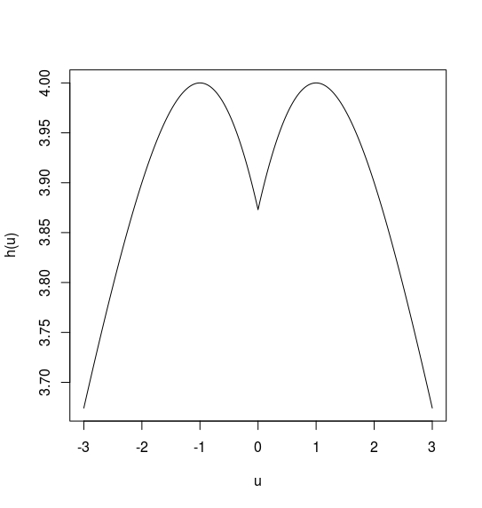
that gives a new proposal. Note that the Sign penalty works like LASSO over all unit vectors and in this sense, it enables the selection of a direction, more than raw variable selection. The Sign penalty produces a thresholding rule, that is, it estimates some coefficients as non–zero. It reaches the minimum when only one of its components is not zero and its maximum when all its components are equal and different from zero. Two important features of this new penalty are that it is scale invariant, so it does not shrink the estimated coefficients as the Elastic Net penalty, and it does not require to select an extra parameter as SCAD and MCP.

3.1 Selection of the penalty parameter

As it is well known, the selection of the penalty parameter is an important practical issue when fitting sparse models, since in some sense it tunes the complexity of the model. This problems has been discussed, among others, in Efron et al. (2004), Meinshausen (2007) and Chi and Scott (2014). In this paper, a robust K−K-fold criterion is used to select the penalty parameter.

As usual, first randomly split the data set into KK disjoint subsets of approximately equal sizes, with indices 𝒞j{\mathcal{C}}_{j}, 1≤j≤K1\leq j\leq K, the j−j-th subset having size nj≥2n_{j}\geq 2, so that ⋃j=1K𝒞j={1,…,n}\bigcup_{j=1}^{K}{\mathcal{C}}_{j}=\{1,\ldots,n\} and ∑j=1Knj=n\sum_{j=1}^{K}n_{j}=n. Let Λ~⊂ℝ\widetilde{\Lambda}\subset\mathbb{R} be the set of possible values for λ\lambda to be considered, and let 𝜷^λ(j)\widehat{\mbox{\boldmath$\beta$}}_{\lambda}^{(j)} be an estimator of 𝜷0\mbox{\boldmath$\beta$}_{0}, computed with penalty parameter λ∈Λ~\lambda\in\widetilde{\Lambda} and without using the observations with indices in 𝒞j{\mathcal{C}}_{j}. For each i=1,…,ni=1,\dots,n, the prediction residuals d^i\widehat{d}_{i} are

d^i,λ=d(yi,𝐱it𝜷^λ(j)),i∈𝒞j,j=1,…,K.\widehat{d}_{i,\lambda}\,=\,d(y_{i},\mathbf{x}_{i}^{\mbox{\footnotesize\sc t}}\widehat{\mbox{\boldmath$\beta$}}_{\lambda}^{(j)})\,,\hskip 9.24994pti\in{\mathcal{C}}_{j}\,,\ j=1,\,\ldots,K\,.

The classical cross–validation criterion constructs adaptive data–driven estimators by minimizing

C​V​(λ)=1n​∑i=1nd^i,λ,CV(\lambda)=\frac{1}{n}\sum_{i=1}^{n}\widehat{d}_{i,\lambda}\,, (14)

an objective function that is usually employed for the classical estimators that involve the minimization of the deviance. However, this criterion is very sensitive to the presence of outliers. In fact, even when 𝜷0\mbox{\boldmath$\beta$}_{0} is estimated by means of a robust method, the traditional cross–validation criterion may lead to poor variable selection results since atypical data may have large prediction residuals that could be very influential on C​V​(λ)CV(\lambda). To overcome this problem, when using robust estimators, it seems natural to use the same loss function ϕ\phi as in (13). Hence, the robust cross-validation criterion selects the penalty parameter by minimizing over Λ~\widetilde{\Lambda}

R​C​V​(λ)=1n​∑1≤j≤K∑i∈𝒞jϕ⁡(yi,𝐱it​𝜷^λ(j))​w​(𝐱i).RCV(\lambda)=\frac{1}{n}\sum_{1\leq j\leq K}\sum_{i\in{\mathcal{C}}_{j}}\phi(y_{i},\mathbf{x}_{i}^{\mbox{\footnotesize\sc t}}\widehat{\mbox{\boldmath$\beta$}}_{\lambda}^{(j)})\,w(\mathbf{x}_{i})\,. (15)

The particular case K=nK=n leads to leave-one-out cross-validation which is a popular choice with a more expensive computational cost. In Section 6, we illustrate through a numerical example, the importance of considering a bounded loss in the cross validation criterion when performing the selection of the penalty parameter.

4 Consistency and order of convergence

In this section, we study the asymptotic behaviour of the estimators defined in (13) when pp is fixed. Even though we are mainly concerned with bounded penalties, our results are general and include among others the Bridge and Elastic Net penalties.

4.1 Assumptions

When considering the function ϕ\phi given in (2), the following set of assumptions on the function ρ\rho are needed.

  1. R1

    ρ:ℝ≥0→ℝ\rho:\mathbb{R}_{\geq 0}\to\mathbb{R} is a bounded, continuously differentiable function with bounded derivative ψ\psi and ρ⁡(0)=0\rho(0)=0.

  2. R2

    ψ⁡(t)≥0\psi(t)\geq 0 and there exists some c≥log⁡2c\geq\log 2 such that ψ⁡(t)>0\psi(t)>0 for all 0<t<c0<t<c.

  3. R3

    ρ\rho is twice continuously differentiable with bounded derivatives, i.e., ψ\psi and ψ′=ρ′′\psi^{\prime}=\rho^{\prime\,\prime} are bounded.

Remark 4.1

Recall that for the estimators defined in (13), ϕ⁡(y,t)=ρ⁡(d⁡(y,t))+G⁡(F⁡(t))+G⁡(1−F⁡(t))\phi(y,t)=\rho(d(y,t))+G(F(t))+G(1-F(t)) and Ψ⁡(y,t)=∂ϕ⁡(y,t)/∂t=−[y−F⁡(t)]​ν​(t)\Psi(y,t)={\partial}\phi(y,t)/{\partial t}=-[y-F(t)]\nu(t) with ν⁡(t)\nu(t) given in (9). Note also that, under R1 and R2, the function Ψ⁡(y,⋅)\Psi(y,\cdot) is continuous and strictly positive.

Denote as χ⁡(y,t)=∂Ψ⁡(y,t)/∂t=F⁡(t)​(1−F⁡(t))​ν​(t)−(y−F⁡(t))​ν′​(t)\chi(y,t)=\partial\Psi(y,t)/\partial t=F(t)(1-F(t))\nu(t)-(y-F(t))\nu^{\prime}(t) and note that χ⁡(0,s)=χ⁡(1,−s)\chi(0,s)=\chi(1,-s). The function χ⁡(y,t)\chi(y,t) always exists for the minimum divergence estimators and is well defined for any function ρ\rho satisfying R3.

It is worth noticing that when ψ⁡(t)>0\psi(t)>0 the constant cc in R2 may be taken as ∞\infty. For instance, this happens when choosing the function ρc\rho_{c} given in (2) or the loss function ρ=ρdiv\rho=\rho_{\mbox{\scriptsize\sc div}} related to the divergence estimators, since their derivatives are always positive. Moreover, when considering the penalized minimum divergence estimators, ρ\rho automatically satisfies conditions R1, R2 and R3. ∎

On the other hand, for the results in this section, the following assumptions regarding the distribution of 𝐱\mathbf{x} are needed.

  1. H1

    For all 𝜶∈ℝp\mbox{\boldmath$\alpha$}\in\mathbb{R}^{p}, 𝜶≠𝟎\mbox{\boldmath$\alpha$}\neq{\bf{0}}, we have ℙ⁡(𝐱t​𝜶=0)=0\mathbb{P}(\mathbf{x}^{\mbox{\footnotesize\sc t}}\mbox{\boldmath$\alpha$}=0)=0.

  2. H2

    ww is a non–negative bounded function with support 𝒞w{\mathcal{C}}_{w} such that ℙ⁡(𝐱∈𝒞w)>0\mathbb{P}(\mathbf{x}\in{\mathcal{C}}_{w})>0. Without loss of generality, we assume that ‖w‖∞=1\|w\|_{\infty}=1.

  3. H3

    𝔼⁡[w⁡(𝐱)​‖𝐱‖2]<∞\mathbb{E}[w(\mathbf{x})\|\mathbf{x}\|^{2}]<\infty.

  4. H4

    The matrix 𝐀\mathbf{A} given in (11) is non–singular.

Remark 4.2

Assumptions H1 and H2 entail that the estimators defined in (6) are Fisher–consistent and will allow to derive consistency results for the estimators defined in (13). H1 holds for instance, when 𝐱\mathbf{x} has a density with support 𝒮{\mathcal{S}} such that 𝒮∩𝒞w≠∅{\mathcal{S}}\cap{\mathcal{C}}_{w}\neq\emptyset. In fact, the weaker assumption ℙ⁡(𝐱t​𝜶=0∪w⁡(𝐱)=0)<1\mathbb{P}(\mathbf{x}^{\mbox{\footnotesize\sc t}}\mbox{\boldmath$\alpha$}=0\cup w(\mathbf{x})=0)<1 for any 𝜶≠𝟎\mbox{\boldmath$\alpha$}\neq{\bf{0}} is enough for obtaining Fisher–consistency. However, in order to ensure consistency a stronger requirement is needed to warranty that the infimum is not attained at infinity. It is worth noticing that H1 entails that 𝔼⁡[w⁡(𝐱)​𝐱𝐱t]\mathbb{E}[w(\mathbf{x})\,\mathbf{x}\mathbf{x}^{\mbox{\footnotesize\sc t}}] is a positive definite matrix. Furthermore, when considering the minimum divergence estimators the matrix 𝐀\mathbf{A} is non–singular, since ℙ⁡(ν⁡(𝐱t​𝜷0)>0)=1\mathbb{P}(\nu(\mathbf{x}^{\mbox{\footnotesize\sc t}}\mbox{\boldmath$\beta$}_{0})>0)=1, so H4 holds. Similarly, when ℙ⁡(𝐱t​𝜶=0)<1\mathbb{P}(\mathbf{x}^{\mbox{\footnotesize\sc t}}\mbox{\boldmath$\alpha$}=0)<1 for any 𝜶≠𝟎\mbox{\boldmath$\alpha$}\neq{\bf{0}}, and ϕ\phi is given by (2) and ψ⁡(t)>0\psi(t)>0 for all tt, as is the case with the loss function introduced in Croux and Haesbroeck (2003), 𝐀\mathbf{A} is non–singular. On the other hand, when R2 holds for some finite positive constant c≥log⁡2c\geq\log 2, 𝐀\mathbf{A} is positive definite when H1 holds. Moreover, define Υ⁡(t)=F⁡(t)​(1−F⁡(t))​ν​(t)\Upsilon(t)=F(t)(1-F(t))\nu(t), straightforward arguments allow to see that 𝐀\mathbf{A} is also non–singular when ℙ⁡(𝐱t​𝜶=0)<1\mathbb{P}(\mathbf{x}^{\mbox{\footnotesize\sc t}}\mbox{\boldmath$\alpha$}=0)<1 holds, for any 𝜶≠𝟎\mbox{\boldmath$\alpha$}\neq{\bf{0}}, and at least one of the following conditions is fulfilled: a) the function 𝔼⁡[w⁡(𝐱)​𝐱𝐱t​1Υ⁡(𝐱t​𝜷0)≥η]\mathbb{E}[w(\mathbf{x})\mathbf{x}\mathbf{x}^{\mbox{\footnotesize\sc t}}\textbf{1}_{\Upsilon(\mathbf{x}^{\mbox{\footnotesize\sc t}}\mbox{\scriptsize${\mbox{\boldmath$\beta$}}$}_{0})\geq\eta}] is continuous in η\eta or b) there exists some c>0c>0 such that ℙ⁡(Υ⁡(𝐱t​𝜷0)>c)=1\mathbb{P}(\Upsilon(\mathbf{x}^{\mbox{\footnotesize\sc t}}\mbox{\boldmath$\beta$}_{0})>c)=1. ∎

4.2 Consistency and rate of convergence

It is worth noticing that, in Theorem 4.1, the parameter λn\lambda_{n} may be deterministic or random and in the latter situation, the only requirement is that Iλn​(𝜷0)⟶a.s.0I_{\lambda_{n}}(\mbox{\boldmath$\beta$}_{0})\mathrel{\mathop{\kern 0.0pt\longrightarrow}\limits^{a.s.}}0. In particular, for the penalties LASSO, Sign, Ridge, Bridge, SCAD and MCP mentioned in Section 3 this condition holds when λn⟶c.s.0\lambda_{n}\mathrel{\mathop{\kern 0.0pt\longrightarrow}\limits^{c.s.}}0.

The next Theorem states the strong consistency of the estimators defined in (13), when considering as function ϕ\phi the function controlling large values of the deviance residuals given in (2).

Theorem 4.1.

Let ϕ:ℝ2→ℝ\phi:\mathbb{R}^{2}\to\mathbb{R} be the function given in (2), where the function ρ:ℝ≥0→ℝ\rho:\mathbb{R}_{\geq 0}\to\mathbb{R} satisfies R1 and R2. Then, if Iλn​(𝛃0)⟶a.s.0I_{\lambda_{n}}(\mbox{\boldmath$\beta$}_{0})\mathrel{\mathop{\kern 0.0pt\longrightarrow}\limits^{a.s.}}0 when n→∞n\to\infty and H1 and H2 hold, we have that the estimator 𝛃^n\widehat{\mbox{\boldmath$\beta$}}_{n} defined in (13) is strongly consistent for 𝛃0\mbox{\boldmath$\beta$}_{0}.

In order to prove the n−\sqrt{n}-consistency of the proposed estimators, we need the following assumption on the penalty function. From now on, ℬ⁡(𝜷,ϵ){\mathcal{B}}(\mbox{\boldmath$\beta$},\epsilon) stands for the closed ball, with respect to the usual ∥⋅∥2\|\cdot\|_{2} norm, centred at 𝜷\beta with radius ϵ\epsilon, i.e., ℬ⁡(𝜷,ϵ)={𝐛∈ℝp:‖𝐛−𝜷‖2≤ϵ}{\mathcal{B}}(\mbox{\boldmath$\beta$},\epsilon)=\{\mathbf{b}\in\mathbb{R}^{p}:\|\mathbf{b}-\mbox{\boldmath$\beta$}\|_{2}\leq\epsilon\}.

  1. P1

    Iλ​(𝜷)/λI_{\lambda}(\mbox{\boldmath$\beta$})/\lambda is Lipschitz in a neighbourhood of 𝜷0\mbox{\boldmath$\beta$}_{0}, that is, there exists ϵ>0\epsilon>0 a constant KK, which does not depend on λ\lambda, such that if 𝜷1,𝜷2∈ℬ⁡(𝜷0,ϵ)\mbox{\boldmath$\beta$}_{1},\mbox{\boldmath$\beta$}_{2}\in{\mathcal{B}}(\mbox{\boldmath$\beta$}_{0},\epsilon) then |Iλ​(𝜷1)−Iλ​(𝜷2)|≤λ​K​‖𝜷1−𝜷2‖1|I_{\lambda}(\mbox{\boldmath$\beta$}_{1})-I_{\lambda}(\mbox{\boldmath$\beta$}_{2})|\leq\lambda K\|\mbox{\boldmath$\beta$}_{1}-\mbox{\boldmath$\beta$}_{2}\|_{1}.

Remark 4.3

Note that the Ridge, Elastic Net, SCAD and MCP penalties satisfy P1, since ‖𝜷‖2≤‖𝜷‖1≤p​‖𝜷‖2\|\mbox{\boldmath$\beta$}\|_{2}\leq\|\mbox{\boldmath$\beta$}\|_{1}\leq\sqrt{p}\,\|\mbox{\boldmath$\beta$}\|_{2}. Furthermore, the Sign penalty also satisfies P1 if ‖𝜷0‖2≠0\|\mbox{\boldmath$\beta$}_{0}\|_{2}\neq 0. Moreover, if Iλ​(𝜷)=λ​∑ℓ=1pJℓ​(|βℓ|)I_{\lambda}(\mbox{\boldmath$\beta$})=\lambda\,\sum_{\ell=1}^{p}J_{\ell}(|\beta_{\ell}|), where Jℓ​(⋅)J_{\ell}(\cdot) is a continuously differentiable function, then IλI_{\lambda} satisfies P1, which implies that the Bridge penalty satisfies P1 for q≥1q\geq 1. ∎

Theorem 4.2.

Let 𝛃^n\widehat{\mbox{\boldmath$\beta$}}_{n} be the estimator defined in (13) with ϕ⁡(y,t)\phi(y,t) given in (2), where the function ρ:ℝ≥0→ℝ\rho:\mathbb{R}_{\geq 0}\to\mathbb{R} satisfies R3. Furthermore, assume that 𝛃^n⟶p𝛃0\widehat{\mbox{\boldmath$\beta$}}_{n}\mathrel{\mathop{\kern 0.0pt\longrightarrow}\limits^{p}}\mbox{\boldmath$\beta$}_{0} and that assumptions H2 to H4 hold.

  1. (a)

    If assumption P1 holds, ‖𝜷^n−𝜷0‖2=Oℙ​(λn+ 1/n)\|\widehat{\mbox{\boldmath$\beta$}}_{n}-\mbox{\boldmath$\beta$}_{0}\|_{2}=O_{\mathbb{P}}(\lambda_{n}\,+\,1/\sqrt{n}). Hence, if λn=Oℙ​(1/n)\lambda_{n}=O_{\mathbb{P}}(1/\sqrt{n}), we have that ‖𝜷^n−𝜷0‖2=Oℙ​(1/n)\|\widehat{\mbox{\boldmath$\beta$}}_{n}-\mbox{\boldmath$\beta$}_{0}\|_{2}=O_{\mathbb{P}}(1/\sqrt{n}), while if λn​n→∞\lambda_{n}\sqrt{n}\to\infty, ‖𝜷^n−𝜷0‖2=Oℙ​(λn)\|\widehat{\mbox{\boldmath$\beta$}}_{n}-\mbox{\boldmath$\beta$}_{0}\|_{2}=O_{\mathbb{P}}(\lambda_{n}).

  2. (b)

    Suppose Iλn​(𝜷)=∑ℓ=1pJλn​(|βℓ|)I_{\lambda_{n}}(\mbox{\boldmath$\beta$})=\sum_{\ell=1}^{p}J_{\lambda_{n}}(|\beta_{\ell}|) where Jλn​(⋅)J_{\lambda_{n}}(\cdot) is two times differentiable in (0,∞)(0,\infty), takes nonnegative values, Jλn′​(|β0,ℓ|)≥0J^{\prime}_{\lambda_{n}}(|\beta_{0,\ell}|)\geq 0 and Jλn​(0)=0J_{\lambda_{n}}(0)=0. Let

    an=max⁡{Jλn′​(|β0,ℓ|):1≤ℓ≤p​and​β0,ℓ≠0}​and​αn=1n+an.a_{n}=\max\,\left\{J^{\prime}_{\lambda_{n}}(|\beta_{0,\ell}|):1\leq\ell\leq p\;\;\text{and}\;\;\beta_{0,\ell}\neq 0\right\}\hskip 9.24994pt\text{and}\hskip 9.24994pt\alpha_{n}=\frac{1}{\sqrt{n}}+a_{n}.

    In addition, assume that there exists some δ>0\delta>0 such that

    sup{|Jλn′′(|β0,ℓ|+τδ)|:τ∈[−1,1], 1≤ℓ≤pandβ0,ℓ≠0}⟶p0.\sup\{|J_{\lambda_{n}}^{\prime\,\prime}(|\beta_{0,\ell}|+\tau\delta)|:\tau\in[-1,1]\;,\;1\leq\ell\leq p\;\;\text{and}\;\;\beta_{0,\ell}\neq 0\}\mathrel{\mathop{\kern 0.0pt\longrightarrow}\limits^{p}}0.

    Then, ‖𝜷^n−𝜷0‖2=Oℙ​(αn)\|\widehat{\mbox{\boldmath$\beta$}}_{n}-\mbox{\boldmath$\beta$}_{0}\|_{2}=O_{\mathbb{P}}(\alpha_{n}).

Remark 4.4

Theorem 4.2(a) shows that, when the penalty satisfies assumption P1, the estimator rate of convergence depend on the convergence rate of λn\lambda_{n} to 0. In particular, if λn​n\lambda_{n}\sqrt{n} is bounded in probability, then the robust penalized consistent estimator has rate n\sqrt{n}, while if λn​n→∞\lambda_{n}\sqrt{n}\to\infty, the convergence rate of 𝜷^n\widehat{\mbox{\boldmath$\beta$}}_{n} is slower than n\sqrt{n}. This result is analogous to the one obtained, under a linear regression model, in Zou (2006) for the penalized least squares estimator when a LASSO penalty is considered. Note that, for the LASSO penalty, the convergence rates obtained in (a) and ( b) are equal since Jλn​(v)=λn​vJ_{\lambda_{n}}(v)=\lambda_{n}\,v. which entails that an=λna_{n}=\lambda_{n} and for any β0,ℓ≠0\beta_{0,\ell}\neq 0, τ∈[−1,1]\tau\in[-1,1], Jλn′′​(|β0,ℓ|+τ​δ)=0J_{\lambda_{n}}^{\prime\prime}(|\beta_{0,\ell}|+\tau\delta)=0 for a smaller enough δ>0\delta>0.

Instead, SCAD and MCP penalties are not only Lipschitz, but based on univariate twice continuously differentiable functions Jλn​(t)J_{\lambda_{n}}(t) satisfying the requirements asked in Theorem 4.2(b) when λn→0\lambda_{n}\to 0. Indeed, for these penalties Jλn′​(t)J^{\prime}_{\lambda_{n}}(t) and Jλn′′​(t)J_{\lambda_{n}}^{\prime\prime}(t) are 0 if t>a​λnt>\,a\,\lambda_{n} where aa is their second tuning constant which is assumed to be fixed. Hence, if λn⟶p0\lambda_{n}\mathrel{\mathop{\kern 0.0pt\longrightarrow}\limits^{p}}0 for any δ>0\delta>0 there exists n0n_{0} such that, for any n≥n0n\geq n_{0}, we have that ℙ⁡(a​λn<m0)>1−δ\mathbb{P}(a\lambda_{n}<m_{0})>1-\delta with m0=min{|β0,ℓ|):1≤ℓ≤pandβ0,ℓ≠0}m_{0}=\min\{|\beta_{0,\ell}|):1\leq\ell\leq p\;\;\text{and}\;\;\beta_{0,\ell}\neq 0\}. Thus, for n≥n0n\geq n_{0}, ℙ⁡(an=0​ and ​bn=0)>1−δ\mathbb{P}(a_{n}=0\mbox{ and }b_{n}=0)>1-\delta and therefore, αn=Oℙ​(1/n)\alpha_{n}=O_{\mathbb{P}}(1/{\sqrt{n}}), implying that the root–nn rate may be achieved only assuming only that λn⟶p0\lambda_{n}\mathrel{\mathop{\kern 0.0pt\longrightarrow}\limits^{p}}0. It is worth noticing that, even when, the Ridge penalty is Lipschitz and it is also based on univariate twice continuously differentiable functions, Jλn′​(|β0,ℓ|)=λn​|β0,ℓ|J^{\prime}_{\lambda_{n}}(|\beta_{0,\ell}|)=\lambda_{n}|\beta_{0,\ell}|, so that an=O⁡(1/n+λn)a_{n}=O(1/\sqrt{n}+\lambda_{n}), leading to root-nn consistency rate with the additional requirement λn=Oℙ​(1/n)\lambda_{n}=O_{\mathbb{P}}(1/\sqrt{n}). The different behaviour of the estimators related to Lipschitz penalties or penalties related to twice continuously differentiable functions with null first derivative for nn large enough, plays an important role regarding the variable selection properties of the procedure. ∎

5 Asymptotic distribution results

The first result in this Section concerns the variable selection properties for our estimator. As shown below the result depends on the behaviour of the penalty function.

Without loss of generality, assume that 𝜷0=(𝜷0,At,𝟎p−kt)t\mbox{\boldmath$\beta$}_{0}=(\mbox{\boldmath$\beta$}_{0,A}^{\mbox{\footnotesize\sc t}},{\bf{0}}_{p-k}^{\mbox{\footnotesize\sc t}})^{\mbox{\footnotesize\sc t}} and 𝜷0,A∈ℝk\mbox{\boldmath$\beta$}_{0,A}\in\mathbb{R}^{k}, k≥1k\geq 1, is the subvector with active coordinates of 𝜷0\mbox{\boldmath$\beta$}_{0} (i.e. the subvector of non–zero elements of 𝜷0\mbox{\boldmath$\beta$}_{0}). We will make use of the notation 𝜷=(𝜷At,𝜷Bt)t\mbox{\boldmath$\beta$}=(\mbox{\boldmath$\beta$}_{A}^{\mbox{\footnotesize\sc t}},\mbox{\boldmath$\beta$}_{B}^{\mbox{\footnotesize\sc t}})^{\mbox{\footnotesize\sc t}}, where 𝜷A∈ℝk\mbox{\boldmath$\beta$}_{A}\in\mathbb{R}^{k} with k≥1k\geq 1 and 𝜷B∈ℝp−k\mbox{\boldmath$\beta$}_{B}\in\mathbb{R}^{p-k}.

When the estimator automatically selects variables, we will be able to show an oracle property, that is, that the penalized M−M-estimator of the non–null components of 𝜷0\mbox{\boldmath$\beta$}_{0}, 𝜷^n,A\widehat{\mbox{\boldmath$\beta$}}_{n,A} has the same asymptotic distribution as that of the estimator obtained assuming that the last components of 𝜷0\mbox{\boldmath$\beta$}_{0} are equal to 00 and using this restriction in the logistic regression model.

5.1 Variable selection property

Theorem 5.1.

Let 𝛃^n=(𝛃^n,At,𝛃^n,Bt)t\widehat{\mbox{\boldmath$\beta$}}_{n}=(\widehat{\mbox{\boldmath$\beta$}}_{n,A}^{\mbox{\footnotesize\sc t}},\widehat{\mbox{\boldmath$\beta$}}_{n,B}^{\mbox{\footnotesize\sc t}})^{\mbox{\footnotesize\sc t}} be the estimator defined in (13), where ϕ⁡(y,t)\phi(y,t) is given in (2) and the function ρ:ℝ≥0→ℝ\rho:\mathbb{R}_{\geq 0}\to\mathbb{R} satisfies R3. Furthermore, assume that H2 and H3 hold and that n​‖𝛃^n−𝛃0‖2=Oℙ​(1)\sqrt{n}\|\widehat{\mbox{\boldmath$\beta$}}_{n}-\mbox{\boldmath$\beta$}_{0}\|_{2}=O_{\mathbb{P}}(1). Furthermore, assume that for every C>0C>0 and ℓ∈{k+1,…,p}\ell\in\{k+1,\dots,p\}, there exist a constant KC,ℓK_{C,\ell} and NC,ℓ∈ℕN_{C,\ell}\in\mathbb{N} such that if ‖𝐮‖2≤C\|\mathbf{u}\|_{2}\leq C and n≥NC,ℓn\geq N_{C,\ell}, then

Iλn​(𝜷0+𝐮n)−Iλn​(𝜷0+𝐮(−ℓ)n)≥KC,ℓ​λnn​|uℓ|,I_{\lambda_{n}}\left(\mbox{\boldmath$\beta$}_{0}+\frac{\mathbf{u}}{\sqrt{n}}\right)-I_{\lambda_{n}}\left(\mbox{\boldmath$\beta$}_{0}+\frac{\mathbf{u}^{(-\ell)}}{\sqrt{n}}\right)\geq K_{C,\ell}\,\frac{\lambda_{n}}{\sqrt{n}}\,|u_{\ell}|, (16)

where 𝐮(−ℓ)\mathbf{u}^{(-\ell)} is obtained by replacing the ℓ−\ell-th coordinate of 𝐮\mathbf{u} with zero and uℓu_{\ell} is the ℓ−\ell-th coordinate of 𝐮\mathbf{u}.

  1. (a)

    For every τ>0\tau>0, there exists b>0b>0 and n0∈ℕn_{0}\in\mathbb{N} such that if λn=b/n\lambda_{n}=b/\sqrt{n}, we have that, for any n≥n0n\geq n_{0},

    ℙ⁡(𝜷^n,B=𝟎p−k)≥1−τ.\mathbb{P}(\widehat{\mbox{\boldmath$\beta$}}_{n,B}={\bf{0}}_{p-k})\geq 1-\tau\,.
  2. (b)

    If λn​n→∞\lambda_{n}\,\sqrt{n}\to\infty, then

    ℙ⁡(𝜷^n,B=𝟎p−k)→1.\mathbb{P}(\widehat{\mbox{\boldmath$\beta$}}_{n,B}={\bf{0}}_{p-k})\to 1\,.

To prove variable selection properties for our estimators, it only remains to show that condition (16) holds for the different penalties mentioned above. First note that (16) is clearly satisfied for the LASSO penalty. In the proof of Corollary 5.2 we show that SCAD, MCP and the Sign penalty also verify (16).

Corollary 5.2.

Let 𝛃^n=(𝛃^n,At,𝛃^n,Bt)t\widehat{\mbox{\boldmath$\beta$}}_{n}=(\widehat{\mbox{\boldmath$\beta$}}_{n,A}^{\mbox{\footnotesize\sc t}},\widehat{\mbox{\boldmath$\beta$}}_{n,B}^{\mbox{\footnotesize\sc t}})^{\mbox{\footnotesize\sc t}} be the estimator defined in (13) with ϕ⁡(y,t)\phi(y,t) given by (2) where the function ρ:ℝ≥0→ℝ\rho:\mathbb{R}_{\geq 0}\to\mathbb{R} satisfies R3. Assume that H2 and H3 hold and n​‖𝛃^n−𝛃0‖2=Oℙ​(1)\sqrt{n}\|\widehat{\mbox{\boldmath$\beta$}}_{n}-\mbox{\boldmath$\beta$}_{0}\|_{2}=O_{\mathbb{P}}(1).

  1. (a)

    If Iλn​(𝜷)I_{\lambda_{n}}(\mbox{\boldmath$\beta$}) is the Sign penalty, then for every τ>0\tau>0 there exist b>0b>0 and n0∈ℕn_{0}\in\mathbb{N} such that if λn=b/n\lambda_{n}=b/\sqrt{n}, we have that, for any n≥n0n\geq n_{0},

    ℙ⁡(𝜷^n,B=𝟎p−k)≥1−τ.\mathbb{P}(\widehat{\mbox{\boldmath$\beta$}}_{n,B}={\bf{0}}_{p-k})\geq 1-\tau\,.
  2. (b)

    If Iλn​(𝜷)I_{\lambda_{n}}(\mbox{\boldmath$\beta$}) is taken as the SCAD or MCP penalties and n​λn→∞\sqrt{n}\lambda_{n}\to\infty, then

    ℙ⁡(𝜷^n,B=𝟎p−k)→1.\mathbb{P}(\widehat{\mbox{\boldmath$\beta$}}_{n,B}={\bf{0}}_{p-k})\to 1.
Remark 5.1

A consequence of Corollary 5.2 is that the penalties SCAD and MCP have the property of automatically selecting variables whenn​λn→∞\sqrt{n}\lambda_{n}\to\infty. In contrast, when using the LASSO and Sign penalties, we cannot ensure the variable selection property when the estimator is root-nn consistent. Recall that, for these two penalties, Theorem 4.2 entails that the estimator converges at a rate slower than n\sqrt{n} when λn​n→∞\lambda_{n}\sqrt{n}\to\infty. For that reason, we can only guarantee that for a given 0<τ<10<\tau<1, we can choose a sequence of penalty parameters λn=b/n\lambda_{n}=b/\sqrt{n} (in order to ensure that the estimator has a root-nn rate) and such that the penalized M−M-estimator selects variables with probability larger than 1−τ1-\tau.

The results in the asymptotic distribution given below will allow to conclude that, for the LASSO and Sign penalties, when the estimator has convergence rate n\sqrt{n}, then lim supnℙ⁡(𝒜n=𝒜)<1\limsup_{n}\mathbb{P}({\mathcal{A}}_{n}={\mathcal{A}})<1, where 𝒜={j:β0,j≠0}={1,…,k}{\mathcal{A}}=\{j:\beta_{0,j}\neq 0\}=\{1,\dots,k\} and 𝒜n={j:β^n,j≠0}{\mathcal{A}}_{n}=\{j:\widehat{\beta}_{n,j}\neq 0\} are the set of index related to the active components of 𝜷0\mbox{\boldmath$\beta$}_{0} and to the non–null coordinates of 𝜷^n\widehat{\mbox{\boldmath$\beta$}}_{n}, respectively. This result is analogous to Proposition 1 in Zou (2006), which shows that the LASSO estimator leads to inconsistent variable selection in the linear regression model, when λn=O⁡(1/n)\lambda_{n}=O(1/\sqrt{n}).

It is worth noticing that 𝜷^n,B=𝟎p−k\widehat{\mbox{\boldmath$\beta$}}_{n,B}={\bf{0}}_{p-k} if and only if 𝒜n⊂𝒜{\mathcal{A}}_{n}\subset{\mathcal{A}}, hence, if ℙ⁡(𝜷^n,B=𝟎p−k)→1\mathbb{P}(\widehat{\mbox{\boldmath$\beta$}}_{n,B}={\bf{0}}_{p-k})\to 1 we have that ℙ⁡(𝒜n⊂𝒜)→1\mathbb{P}({\mathcal{A}}_{n}\subset{\mathcal{A}})\to 1. Note that when 𝒜n⊊𝒜{\mathcal{A}}_{n}\subsetneq{\mathcal{A}}, the penalized M−M-estimator may select a submodel with less predictors than the original one, shrinking the estimation of some of the active to 00; however, the oracle property of the estimators based on SCAD or MCP given in Theorem 5.7 will allow to conclude that ℙ⁡(𝒜n=𝒜)→1\mathbb{P}({\mathcal{A}}_{n}={\mathcal{A}})\to 1. ∎

5.2 Asymptotic distribution

In this section, we derive separately the asymptotic distribution of our estimator depending on the choice of the penalty. As the rate of convergence to 00 of λn\lambda_{n} required to obtain root−n-n estimators for the Sign is different from that of SCAD or MCP penalties, we will study these two situations separately. Even though most results on penalized estimators assume that the sequence of penalty parameters is deterministic, in this section, as in Theorem 4.2, we will allow random penalty parameters λn\lambda_{n}, having in this sense a more realistic point of view.

It is worth noticing that, under H4, the matrix 𝐀\mathbf{A} defined in (11) is positive definite, so the submatrix corresponding to the active coordinates of 𝜷0\mbox{\boldmath$\beta$}_{0} is also positive definite.

From now on, 𝐞ℓ\mathbf{e}_{\ell} stands for the ℓ−\ell-th canonical vector and sign​(z){\mbox{\rm sign}}(z) is the univariate sign function, that is, sign​(z)=z/|z|{\mbox{\rm sign}}(z)=z/|z| when z≠0z\neq 0 and sign​(0)=0{\mbox{\rm sign}}(0)=0.

Theorem 5.3.

Let 𝛃^n\widehat{\mbox{\boldmath$\beta$}}_{n} be the estimator defined in (13) with ϕ⁡(y,t)\phi(y,t) given in (2), where the function ρ:ℝ≥0→ℝ\rho:\mathbb{R}_{\geq 0}\to\mathbb{R} satisfies R3. Assume that H2 to H4 hold, n​(𝛃^n−𝛃0)=Oℙ​(1)\sqrt{n}(\widehat{\mbox{\boldmath$\beta$}}_{n}-\mbox{\boldmath$\beta$}_{0})=O_{\mathbb{P}}(1) and n​λn⟶pb\sqrt{n}\,\lambda_{n}\mathrel{\mathop{\kern 0.0pt\longrightarrow}\limits^{p}}b. Consider the Sign penalty given by

Iλ​(𝜷)=λ​‖𝜷‖1‖𝜷‖2=λ​∑ℓ=1p|βℓ|‖𝜷‖2.I_{\lambda}(\mbox{\boldmath$\beta$})=\lambda\,\frac{\|\mbox{\boldmath$\beta$}\|_{1}}{\|\mbox{\boldmath$\beta$}\|_{2}}=\lambda\,\sum_{\ell=1}^{p}\frac{|\beta_{\ell}|}{\|\mbox{\boldmath$\beta$}\|_{2}}\,.

Then, if ‖𝛃0‖≠0\|\mbox{\boldmath$\beta$}_{0}\|\neq 0, n​(𝛃^n−𝛃0)⟶Dargmin𝐳⁡R⁡(𝐳)\sqrt{n}(\widehat{\mbox{\boldmath$\beta$}}_{n}-\mbox{\boldmath$\beta$}_{0})\mathrel{\mathop{\kern 0.0pt\longrightarrow}\limits^{D}}\mathop{\mbox{\rm argmin}}_{\mathbf{z}}R(\mathbf{z}), where the process R:ℝp→ℝR:\mathbb{R}^{p}\to\mathbb{R} is defined as

R⁡(𝐳)=𝐳t​𝐰+𝐳t​𝐀𝐳+b​𝐳t​𝐪​(𝐳),R(\mathbf{z})=\mathbf{z}^{\mbox{\footnotesize\sc t}}\mathbf{w}+\mathbf{z}^{\mbox{\footnotesize\sc t}}\mathbf{A}\mathbf{z}+b\;\mathbf{z}^{\mbox{\footnotesize\sc t}}\mathbf{q}(\mathbf{z})\,,

with 𝐰∼Np​(𝟎,𝐁)\mathbf{w}\sim N_{p}({\bf{0}},\mathbf{B}), 𝐀\mathbf{A} and 𝐁\mathbf{B} are given in (11) and (12), respectively and

𝐪⁡(𝐳)\displaystyle\mathbf{q}(\mathbf{z}) =\displaystyle= ∑ℓ=1p∇Jℓ(𝜷0)1{β0,ℓ≠0}+sign​(zℓ)‖𝜷0‖21{β0,ℓ=0}𝐞ℓ,\displaystyle\sum_{\ell=1}^{p}\nabla J_{\ell}(\mbox{\boldmath$\beta$}_{0})\textbf{1}_{\{\beta_{0,\ell}\neq 0\}}+\frac{{\mbox{\rm sign}}(z_{\ell})}{\|\mbox{\boldmath$\beta$}_{0}\|_{2}}\textbf{1}_{\{\beta_{0,\ell}=0\}}\,\mathbf{e}_{\ell}\,,
∇Jℓ​(𝜷)\displaystyle\nabla J_{\ell}(\mbox{\boldmath$\beta$}) =\displaystyle= (−|βℓ|​β1‖𝜷‖23,−|βℓ|​β2‖𝜷‖23,…,sign​(βℓ)​‖𝜷‖22−βℓ2‖𝜷‖23,…,−|βℓ|​βp‖𝜷‖23)\displaystyle\left(-\frac{|\beta_{\ell}|\beta_{1}}{\|\mbox{\boldmath$\beta$}\|_{2}^{3}},-\frac{|\beta_{\ell}|\beta_{2}}{\|\mbox{\boldmath$\beta$}\|_{2}^{3}},\dots,{\mbox{\rm sign}}(\beta_{\ell})\frac{\|\mbox{\boldmath$\beta$}\|_{2}^{2}-\beta_{\ell}^{2}}{\|\mbox{\boldmath$\beta$}\|_{2}^{3}},\dots,-\frac{|\beta_{\ell}|\beta_{p}}{\|\mbox{\boldmath$\beta$}\|_{2}^{3}}\right)
=\displaystyle= −|βℓ|‖𝜷‖23​𝜷+sign​(βℓ)‖𝜷‖2​𝐞ℓ\displaystyle\,-\,\frac{|\beta_{\ell}|}{\|\mbox{\boldmath$\beta$}\|_{2}^{3}}\,\mbox{\boldmath$\beta$}\,+\,\frac{{\mbox{\rm sign}}(\beta_{\ell})}{\|\mbox{\boldmath$\beta$}\|_{2}}\,\mathbf{e}_{\ell}

where Jℓ​(𝛃)=|βℓ|/‖𝛃‖2J_{\ell}(\mbox{\boldmath$\beta$})=|\beta_{\ell}|/\|\mbox{\boldmath$\beta$}\|_{2}.

The following result generalizes Theorem 5.3 to differentiable penalties and includes, among others, the LASSO and Ridge penalties, and any convex combination of them, in particular the Elastic Net.

Theorem 5.4.

Let 𝛃^n\widehat{\mbox{\boldmath$\beta$}}_{n} be the estimator defined in (13) with ϕ⁡(y,t)\phi(y,t) given by (2), where the function ρ:ℝ≥0→ℝ\rho:\mathbb{R}_{\geq 0}\to\mathbb{R} satisfies R3 and let 𝐀\mathbf{A} and 𝐁\mathbf{B} be the matrices defined in (11) and (12), respectively. Let us consider the penalty given by

Iλ​(𝜷)=λ⁡{(1−α)​∑ℓ=1pJℓ​(|βℓ|)+α​∑ℓ=1p|βℓ|},I_{\lambda}(\mbox{\boldmath$\beta$})=\lambda\,\left\{(1-\alpha)\sum_{\ell=1}^{p}J_{\ell}(|\beta_{\ell}|)+\alpha\sum_{\ell=1}^{p}|\beta_{\ell}|\right\}\,, (17)

where Jℓ​(⋅)J_{\ell}(\cdot) is a continuously differentiable function such that Jℓ′​(0)=0J_{\ell}^{\prime}(0)=0. Assume that H2 to H4 hold, n​(𝛃^n−𝛃0)=Oℙ​(1)\sqrt{n}(\widehat{\mbox{\boldmath$\beta$}}_{n}-\mbox{\boldmath$\beta$}_{0})=O_{\mathbb{P}}(1) and that n​λn⟶pb\sqrt{n}\,\lambda_{n}\mathrel{\mathop{\kern 0.0pt\longrightarrow}\limits^{p}}b. Then, if ‖𝛃0‖≠0\|\mbox{\boldmath$\beta$}_{0}\|\neq 0, n​(𝛃^n−𝛃0)⟶Dargmin𝐳⁡R⁡(𝐳)\sqrt{n}(\widehat{\mbox{\boldmath$\beta$}}_{n}-\mbox{\boldmath$\beta$}_{0})\mathrel{\mathop{\kern 0.0pt\longrightarrow}\limits^{D}}\mathop{\mbox{\rm argmin}}_{\mathbf{z}}R(\mathbf{z}) where the process R:ℝp→ℝR:\mathbb{R}^{p}\to\mathbb{R} is defined as

R⁡(𝐳)=𝐳t​𝐰+12​𝐳t​𝐀𝐳+b​𝐳t​𝐪​(𝐳),R(\mathbf{z})=\mathbf{z}^{\mbox{\footnotesize\sc t}}\mathbf{w}+\frac{1}{2}\,\mathbf{z}^{\mbox{\footnotesize\sc t}}\mathbf{A}\mathbf{z}+b\;\mathbf{z}^{\mbox{\footnotesize\sc t}}\mathbf{q}(\mathbf{z})\,,

with 𝐰∼Np​(𝟎,𝐁)\mathbf{w}\sim N_{p}({\bf{0}},\mathbf{B}) and 𝐪⁡(𝐳)=(q1​(𝐳),…,qp​(𝐳))t\mathbf{q}(\mathbf{z})=(q_{1}(\mathbf{z}),\dots,q_{p}(\mathbf{z}))^{\mbox{\footnotesize\sc t}} being

qℓ​(𝐳)\displaystyle q_{\ell}(\mathbf{z}) =\displaystyle= (1−α)Jℓ′(|β0,ℓ|)sign(β0,ℓ)+α{sign(β0,ℓ)1{β0,ℓ≠0}+sign(zℓ)1{β0,ℓ=0}}.\displaystyle(1-\alpha)J_{\ell}^{\prime}(|\beta_{0,\ell}|)\;{\mbox{\rm sign}}(\beta_{0,\ell})+\alpha\left\{{\mbox{\rm sign}}(\beta_{0,\ell})\textbf{1}_{\{\beta_{0,\ell}\neq 0\}}+{\mbox{\rm sign}}(z_{\ell})\textbf{1}_{\{\beta_{0,\ell}=0\}}\right\}\,.
Remark 5.2

Note that when n​λn⟶p0\sqrt{n}\lambda_{n}\mathrel{\mathop{\kern 0.0pt\longrightarrow}\limits^{p}}0 (b=0b=0), the penalized estimators based on the Sign penalty or on a penalty of the form (17) have the same asymptotic distribution as the M−M-estimators defined through (6). If b>0b>0 and α>0\alpha>0 in (17), analogous arguments to those considered in linear regression by Knight and Fu (2000), allow to show that the asymptotic distribution of the coordinates of 𝜷^n\widehat{\mbox{\boldmath$\beta$}}_{n} corresponding to null coefficients of 𝜷0\mbox{\boldmath$\beta$}_{0}, that is, the asymptotic distribution of 𝜷^n,B\widehat{\mbox{\boldmath$\beta$}}_{n,B} puts positive probability at zero. On the other hand, if α=0\alpha=0 and b>0b>0, the amount of shrinkage of the estimated regression coefficients increases with the magnitude of the true regression coefficients. Hence, for “large” parameters, the bias introduced by the differentiable penalty Jℓ​(⋅)J_{\ell}(\cdot) may be large.

It is worth noticing that Theorem 5.4 implies that, when Iλ​(𝜷)=λ​∑ℓ=1pJℓ​(|βℓ|)I_{\lambda}(\mbox{\boldmath$\beta$})=\lambda\,\sum_{\ell=1}^{p}J_{\ell}(|\beta_{\ell}|) and n​λn⟶pb\sqrt{n}\lambda_{n}\mathrel{\mathop{\kern 0.0pt\longrightarrow}\limits^{p}}b, n​(𝜷^n−𝜷0)⟶D𝐀−1​(𝐰+b​𝐚)\sqrt{n}(\widehat{\mbox{\boldmath$\beta$}}_{n}-\mbox{\boldmath$\beta$}_{0})\mathrel{\mathop{\kern 0.0pt\longrightarrow}\limits^{D}}\mathbf{A}^{-1}\left(\mathbf{w}+b\mathbf{a}\right), where 𝐚=(a1,…,ap)t\mathbf{a}=(a_{1},\dots,a_{p})^{\mbox{\footnotesize\sc t}} is such that aℓ=Jℓ′​(|β0,ℓ|)​sign​(β0,ℓ)a_{\ell}=J_{\ell}^{\prime}(|\beta_{0,\ell}|)\;{\mbox{\rm sign}}(\beta_{0,\ell}), which shows the existing asymptotic bias introduced in the limiting distribution, unless b=0b=0. In particular, the robust Ridge M−M-estimator, that provides a robust alternative under collinearity, is asymptotically normally distributed as Np​(2​b​𝐀−1​𝜷0,𝐀−1​𝐁𝐀−1)N_{p}(2\,b\,\mathbf{A}^{-1}\mbox{\boldmath$\beta$}_{0},\mathbf{A}^{-1}\mathbf{B}\mathbf{A}^{-1}). ∎

When considering the Sign and LASSO penalties, analogous arguments to those considered in the proof of Proposition 1 in Zou (2006), together with Theorems 5.3 and 5.4 allow to see that, if the penalized M−M-estimator has a root−n-n rate of convergence, then it is inconsistent for variable selection (see Corollary 5.5). Furthermore, from the proof we may conclude that if n​λn⟶p0\sqrt{n}\lambda_{n}\mathrel{\mathop{\kern 0.0pt\longrightarrow}\limits^{p}}0, then ℙ⁡(𝒜n=𝒜)→0\mathbb{P}({\mathcal{A}}_{n}={\mathcal{A}})\to 0, that is, we need regularization parameters that converge to 00, but not too fast in order to select variables with non–null probability.

Corollary 5.5.

Let 𝛃^n=(𝛃^n,At,𝛃^n,Bt)t\widehat{\mbox{\boldmath$\beta$}}_{n}=(\widehat{\mbox{\boldmath$\beta$}}_{n,A}^{\mbox{\footnotesize\sc t}},\widehat{\mbox{\boldmath$\beta$}}_{n,B}^{\mbox{\footnotesize\sc t}})^{\mbox{\footnotesize\sc t}} be the estimator defined in (13), where ϕ⁡(y,t)\phi(y,t) is given through (2) with the function ρ:ℝ≥0→ℝ\rho:\mathbb{R}_{\geq 0}\to\mathbb{R} satisfying R3. Assume that ‖𝛃0‖≠0\|\mbox{\boldmath$\beta$}_{0}\|\neq 0, n​λn⟶pb\sqrt{n}\lambda_{n}\mathrel{\mathop{\kern 0.0pt\longrightarrow}\limits^{p}}b, n​‖𝛃^n−𝛃0‖2=Oℙ​(1)\sqrt{n}\|\widehat{\mbox{\boldmath$\beta$}}_{n}-\mbox{\boldmath$\beta$}_{0}\|_{2}=O_{\mathbb{P}}(1) and that H2 to H4 hold. Then, for the Sign or LASSO penalties, there exists c<1c<1 such that lim supnℙ⁡(𝒜n=𝒜)≤c<1\limsup_{n}\mathbb{P}({\mathcal{A}}_{n}={\mathcal{A}})\leq c<1, where 𝒜={j:β0,j≠0}{\mathcal{A}}=\{j:\beta_{0,j}\neq 0\} is the set of indexes corresponding to the active coordinates of 𝛃0\mbox{\boldmath$\beta$}_{0} and 𝒜n={j:β^n,j≠0}{\mathcal{A}}_{n}=\{j:\widehat{\beta}_{n,j}\neq 0\}.

Similar arguments to those considered in the proof of Theorem5.3, allow to obtain the asymptotic distribution of the penalized M−M-estimator with Sign penalty when n​λn→∞\sqrt{n}\lambda_{n}\to\infty. A similar result holds for penalizations satisfying (17), as the LASSO one.

Theorem 5.6.

Let 𝛃^n\widehat{\mbox{\boldmath$\beta$}}_{n} be the estimator defined in (13), where ϕ⁡(y,t)\phi(y,t) is given through (2) with the function ρ:ℝ≥0→ℝ\rho:\mathbb{R}_{\geq 0}\to\mathbb{R} satisfying R3. Assume that ‖𝛃0‖≠0\|\mbox{\boldmath$\beta$}_{0}\|\neq 0, n​λn⟶p∞\sqrt{n}\lambda_{n}\mathrel{\mathop{\kern 0.0pt\longrightarrow}\limits^{p}}\infty, 𝛃^n−𝛃0=Oℙ​(λn)\widehat{\mbox{\boldmath$\beta$}}_{n}-\mbox{\boldmath$\beta$}_{0}=O_{\mathbb{P}}(\lambda_{n}) and that H2 to H4 hold. Let 𝐀\mathbf{A} be the matrix defined in (11) and consider the Sign penalty

Iλ​(𝜷)=λ​‖𝜷‖1‖𝜷‖2.I_{\lambda}(\mbox{\boldmath$\beta$})=\lambda\,\frac{\|\mbox{\boldmath$\beta$}\|_{1}}{\|\mbox{\boldmath$\beta$}\|_{2}}\,.

Then, (1/λn)​(𝛃^n−𝛃0)⟶pargmin𝐳⁡R⁡(𝐳)(1/\lambda_{n})\;(\widehat{\mbox{\boldmath$\beta$}}_{n}-\mbox{\boldmath$\beta$}_{0})\mathrel{\mathop{\kern 0.0pt\longrightarrow}\limits^{p}}\mathop{\mbox{\rm argmin}}_{\mathbf{z}}R(\mathbf{z}), where the function R:ℝp→ℝR:\mathbb{R}^{p}\to\mathbb{R} is defined through

R⁡(𝐳)=12​𝐳t​𝐀𝐳+𝐳t​𝐪​(𝐳),R(\mathbf{z})=\frac{1}{2}\mathbf{z}^{\mbox{\footnotesize\sc t}}\mathbf{A}\mathbf{z}+\mathbf{z}^{\mbox{\footnotesize\sc t}}\mathbf{q}(\mathbf{z})\,,

with 𝐪⁡(𝐳)\mathbf{q}(\mathbf{z}) the function defined in Theorem 5.3.

Remark 5.3

Lemma 3 in Zou (2006) provides a result analogous to Theorem 5.6 for the LASSO least squares estimator, under a linear regression model. As in that result, the rate of convergence of 𝜷^n\widehat{\mbox{\boldmath$\beta$}}_{n} is slower than n\sqrt{n} and the limit is a non–random quantity. As noted in Zou (2006), the optimal rate for 𝜷^n\widehat{\mbox{\boldmath$\beta$}}_{n} is obtained when λn=Oℙ​(1/n)\lambda_{n}=O_{\mathbb{P}}(1/\sqrt{n}), but at expenses of not selecting variables. ∎

Finally, the following theorem gives the asymptotic distribution of 𝜷^n,A\widehat{\mbox{\boldmath$\beta$}}_{n,A} when the penalty is consistent for variable selection, that is, when ℙ⁡(𝜷^n,B=𝟎p−k)→1\mathbb{P}(\widehat{\mbox{\boldmath$\beta$}}_{n,B}={\bf{0}}_{p-k})\to 1. For that purpose, recall that 𝜷0=(𝜷0,At,𝟎p−kt)t\mbox{\boldmath$\beta$}_{0}=(\mbox{\boldmath$\beta$}_{0,A}^{\mbox{\footnotesize\sc t}},{\bf{0}}_{p-k}^{\mbox{\footnotesize\sc t}})^{\mbox{\footnotesize\sc t}} where 𝜷0,A∈ℝk\mbox{\boldmath$\beta$}_{0,A}\in\mathbb{R}^{k}, k≥1k\geq 1, is the vector of active coordinates of 𝜷0\mbox{\boldmath$\beta$}_{0} and for 𝐛∈ℝk\mathbf{b}\in\mathbb{R}^{k}, define

∇Iλ​(𝐛)=∂Iλ​((𝐛t,𝟎p−kt)t)∂𝐛.\nabla I_{\lambda}(\mathbf{b})=\frac{\partial I_{\lambda}\left((\mathbf{b}^{\mbox{\footnotesize\sc t}},{\bf{0}}_{p-k}^{\mbox{\footnotesize\sc t}})^{\mbox{\footnotesize\sc t}}\right)}{\partial\mathbf{b}}\,.
Theorem 5.7.

Let 𝛃^n\widehat{\mbox{\boldmath$\beta$}}_{n} be the estimator defined in (13) with ϕ⁡(y,t)\phi(y,t) given in (2), where the function ρ:ℝ≥0→ℝ\rho:\mathbb{R}_{\geq 0}\to\mathbb{R} satisfies R3 and assume that H2 and H3 hold. Suppose that there exists some δ>0\delta>0 such that

sup‖𝜷A−𝜷0,A‖2≤δ‖∇Iλn​(𝜷A)‖2=o⁡(1n),\sup_{\|\mbox{\scriptsize${\mbox{\boldmath$\beta$}}$}_{A}-\mbox{\scriptsize${\mbox{\boldmath$\beta$}}$}_{0,A}\|_{2}\leq\delta}\|\nabla I_{\lambda_{n}}(\mbox{\boldmath$\beta$}_{A})\|_{2}=o\left(\frac{1}{\sqrt{n}}\right), (18)

ℙ⁡(𝜷^n,B=𝟎p−k)→1\mathbb{P}(\widehat{\mbox{\boldmath$\beta$}}_{n,B}={\bf{0}}_{p-k})\to 1 and 𝛃^n⟶p𝛃0\widehat{\mbox{\boldmath$\beta$}}_{n}\mathrel{\mathop{\kern 0.0pt\longrightarrow}\limits^{p}}\mbox{\boldmath$\beta$}_{0}. Let 𝐀~\widetilde{\mathbf{A}} and 𝐁~\widetilde{\mathbf{B}} be the k×kk\times k submatrices of 𝐀\mathbf{A} and 𝐁\mathbf{B}, respectively, corresponding to the first kk coordinates of 𝛃0\mbox{\boldmath$\beta$}_{0}, where 𝐀\mathbf{A} and 𝐁\mathbf{B} were defined in (11) and (12). Then, if 𝐀~\widetilde{\mathbf{A}} is invertible,

n​(𝜷^n,A−𝜷0,A)⟶DNk​(𝟎,𝐀~−1​𝐁~​𝐀~−1).\sqrt{n}(\widehat{\mbox{\boldmath$\beta$}}_{n,A}-\mbox{\boldmath$\beta$}_{0,A})\mathrel{\mathop{\kern 0.0pt\longrightarrow}\limits^{D}}N_{k}({\bf{0}},\widetilde{\mathbf{A}}^{-1}\widetilde{\mathbf{B}}\widetilde{\mathbf{A}}^{-1}).
Remark 5.4

Penalties SCAD and MCP fulfil (18) when λn→0\lambda_{n}\to 0. Effectively, recall that any of them may be written as Iλ​(𝜷)=∑j=1pJλ​(|βj|)I_{\lambda}(\mbox{\boldmath$\beta$})=\sum_{j=1}^{p}J_{\lambda}(|\beta_{j}|), where Jλ​(t)J_{\lambda}(t) is constant in [a​λ,∞)[a\lambda,\infty), with a>0a>0 the second tuning constant of these penalties. Using that Jλ​(0)=0J_{\lambda}(0)=0, we obtain that, for any 𝐛∈ℝk\mathbf{b}\in\mathbb{R}^{k}, Iλ​((𝐛t,𝟎p−kt)t)=∑j=1kJλ​(|bj|)I_{\lambda}\left((\mathbf{b}^{\mbox{\footnotesize\sc t}},{\bf{0}}_{p-k}^{\mbox{\footnotesize\sc t}})^{\mbox{\footnotesize\sc t}}\right)=\sum_{j=1}^{k}J_{\lambda}(|b_{j}|) and ∇Iλ​(𝐛)=∑j=1kJλ′​(|bj|)\nabla I_{\lambda}(\mathbf{b})=\sum_{j=1}^{k}J^{\prime}_{\lambda}(|b_{j}|). Since ‖𝜷^−𝜷0‖2=Oℙ​(1/n)\|\widehat{\mbox{\boldmath$\beta$}}-\mbox{\boldmath$\beta$}_{0}\|_{2}=O_{\mathbb{P}}\left(1/\sqrt{n}\right), given δ>0\delta>0 there exists C1>0C_{1}>0 such that ℙ⁡(𝒟n)>1−δ\mathbb{P}({\mathcal{D}}_{n})>1-\delta for n≥n0n\geq n_{0}, with 𝒟n={∥𝜷^−𝜷0∥2≤C1/n}{\mathcal{D}}_{n}=\{\|\widehat{\mbox{\boldmath$\beta$}}-\mbox{\boldmath$\beta$}_{0}\|_{2}\leq C_{1}/\sqrt{n}\}.

Let n1n_{1} be such that C1/n≤m0/2C_{1}/\sqrt{n}\leq m_{0}/2. Then, for any ω∈𝒟n\omega\in{\mathcal{D}}_{n}, n≥n1n\geq n_{1} and 1≤j≤k1\leq j\leq k, we have that

|β^j|≥|β0,j|−|β^j−β0,j|≥m0−C1n≥m02.|\widehat{\beta}_{j}|\geq|\beta_{0,j}|-|\widehat{\beta}_{j}-\beta_{0,j}|\geq m_{0}-\frac{C_{1}}{\sqrt{n}}\geq\frac{m_{0}}{2}\,.

Using that λn→0\lambda_{n}\to 0 we get that for n≥max⁡{n0,n1}n\geq\max\{n_{0},n_{1}\}, we have that j=1,…,kj=1,\ldots,k, |β^j|>a​λn|\widehat{\beta}_{j}|>a\lambda_{n}, implying that 𝒟n⊂{∥∇Iλn(𝜷^A)∥2=0}{\mathcal{D}}_{n}\subset\{\|\nabla I_{\lambda_{n}}(\widehat{\mbox{\boldmath$\beta$}}_{A})\|_{2}=0\} as desired.

Hence, using Corollary 5.2, we get that the penalized M−M-estimators defined through (13) have the oracle property when using SCAD or MCP and λn→0\lambda_{n}\to 0 with n​λn→∞\sqrt{n}\;\lambda_{n}\to\infty. ∎

6 Monte Carlo study

In this section, we present the results of a Monte Carlo study designed to compare the small sample performance of classical and robust penalized estimators. Section 6.1 describes the algorithm used to compute the robust penalized estimators, while the simulation settings and the obtained results are summarized in Section 6.2.

6.1 Algorithm

The algorithm used to compute the estimators proposed in Section 3 is an implementation of the cyclical descent algorithm. Taking into account that the estimators defined in (13) depend on a penalty parameter which is usually chosen by cross–validation , we set a grid of candidates Λ~={λ1,λ2,…,λK}\widetilde{\Lambda}=\{\lambda_{1},\lambda_{2},\dots,\lambda_{K}\}. Given λk∈Λ~\lambda_{k}\in\widetilde{\Lambda} and a subset of indexes ℐk⊂{1,…,p}{\mathcal{I}}_{k}\subset\{1,\dots,p\}, the algorithm consists on the following steps:

  1. (a)

    Obtain an initial estimator 𝜷^ini\widehat{\mbox{\boldmath$\beta$}}_{\mbox{\footnotesize\sc ini}} and define M(0)=Mn​(𝜷^ini)M^{(0)}=M_{n}(\widehat{\mbox{\boldmath$\beta$}}_{\mbox{\footnotesize\sc ini}}), where Mn​(𝜷)=Ln​(𝜷)+Iλ​(𝜷)M_{n}(\mbox{\boldmath$\beta$})=L_{n}(\mbox{\boldmath$\beta$})+I_{\lambda}(\mbox{\boldmath$\beta$}) is given in (13). Fix initially ℓ=0\ell=0.

  2. (b)

    ℓ←ℓ+1\ell\leftarrow\ell+1

    1. Step 1

      Choose a random permutation of the elements of ℐk{\mathcal{I}}_{k}, say i1,…,isi_{1},\dots,i_{s}, where ss is the number of elements of ℐk{\mathcal{I}}_{k}. Following the order given by the indexes of the permutation, minimize the function Mn​(𝜷)M_{n}(\mbox{\boldmath$\beta$}) over one coordinate of 𝜷\beta each at a time, while leaving fixed the remaining ones. This procedure involves ss minimization steps. Denote as 𝜷~\widetilde{\mbox{\boldmath$\beta$}} the obtained value after passing through all the coordinates in ℐk{\mathcal{I}}_{k}.

    2. Step 2

      Choose the value c>0c>0 that minimizes the function Mn​(c​𝜷~)M_{n}(c\,\widetilde{\mbox{\boldmath$\beta$}}). Denote c~\widetilde{c} the resulting value, 𝜷(ℓ)=c~​𝜷~\mbox{\boldmath$\beta$}^{(\ell)}=\widetilde{c}\,\widetilde{\mbox{\boldmath$\beta$}} and M(ℓ)=Mn​(𝜷(ℓ))M^{(\ell)}=M_{n}(\mbox{\boldmath$\beta$}^{(\ell)})

    3. Step 3

      Compute R(ℓ)=|M(ℓ−1)−M(ℓ)|/M(ℓ)R^{(\ell)}=|M^{(\ell-1)}-M^{(\ell)}|/M^{(\ell)}.

  3. (c)

    If the ratio R(ℓ)R^{(\ell)} is smaller than a fixed tolerance parameter, define 𝜷^=𝜷(ℓ)\widehat{\mbox{\boldmath$\beta$}}=\mbox{\boldmath$\beta$}^{(\ell)}, otherwise go back to (b).

When the model includes an intercept, an intermediate step between Steps 1 and 2 is introduced in order to get an intercept estimate by minimizing the objective function only over the intercept parameter, while keeping fixed the value of 𝜷^=𝜷(ℓ)\widehat{\mbox{\boldmath$\beta$}}=\mbox{\boldmath$\beta$}^{(\ell)} obtained in Step 2.

It is worth noting that, in our numerical studies, the univariate optimization in Steps 1 and 2 are carried out using the function optim in R, which implements the Nelder–Mead optimization method. A key point is the choice of the initial estimator 𝜷^ini\widehat{\mbox{\boldmath$\beta$}}_{\mbox{\footnotesize\sc ini}}. Recall that Chi and Scott (2014) based their initial estimator choice on the Karush–Kuhn–Tucker (KKT) conditions for the problem of minimizing argmin𝜷∈ℝp⁡(1/n)​∑i=1n(yi−F⁡(𝐱it​𝜷))2+λ​‖𝜷‖1\mathop{\mbox{\rm argmin}}_{\mbox{\scriptsize${\mbox{\boldmath$\beta$}}$}\in\mathbb{R}^{p}}(1/n)\sum_{i=1}^{n}(y_{i}-F(\mathbf{x}_{i}^{\mbox{\footnotesize\sc t}}\mbox{\boldmath$\beta$}))^{2}+\lambda\|\mbox{\boldmath$\beta$}\|_{1}\,. For j=1,…,pj=1,\dots,p, those authors compute the scores zj=|y¯​(1−y¯)​𝐱(j)t​(𝐲−y¯​𝟏n)|z_{j}=\left|\overline{y}(1-\overline{y})\mathbf{x}_{(j)}^{\mbox{\footnotesize\sc t}}(\mathbf{y}-\overline{y}{\bf{1}}_{n})\right|, where y¯=∑i=1nyi/n\overline{y}=\sum_{i=1}^{n}y_{i}/n, 𝐲=(y1,…,yn)t\mathbf{y}=(y_{1},\dots,y_{n})^{\mbox{\footnotesize\sc t}} and 𝐱(j)\mathbf{x}_{(j)} is the j−j-th column of 𝐱\mathbf{x}. Their initial estimator is based on the response variables with the highest scores (in absolute value) which are set to 1, the remaining ones being set to 0.

When the sample has no contamination, this initial estimator seems to be a good choice (see Chi and Scott, 2014). However, this method may be influenced by outliers as those added in our numerical study. To overcome this drawback, we first compute the quantities κi​j=xi​j​(yi−y¯)\kappa_{ij}=x_{ij}(y_{i}-\overline{y}), 1≤j≤p1\leq j\leq p, 1≤i≤n1\leq i\leq n. Then, for every j=1,…,pj=1,\dots,p, the score z~j\widetilde{z}_{j} is evaluated as the absolute value of the α−\alpha-trimmed mean of {κ1​j,κ2​j,…,κn​j}\{\kappa_{1j},\kappa_{2j},\dots,\kappa_{nj}\}. In our simulation study, we fixed α=0.15\alpha=0.15. Finally, we choose the proportion 0<τ<10<\tau<1 of variables with highest absolute score and we apply the weighted estimator introduced in (7) with the ρ−\rho-function of Croux and Haesbroeck (2003) given in (2) on these selected variables. In our experimental results we have chosen the proportion τ=0.1\tau=0.1.

As mentioned above, the penalty parameter selection is an important step to effectively implement the computation of the procedure in sparse models. This fact and the necessity of a robust cross–validation criterion are discussed in Section 3.1. Therefore, in our study we determine the penalty parameter by minimizing of the traditional criterion C​V​(λ)CV(\lambda) given in (14) when using the classical estimators, while for the robust ones we consider R​C​V​(λ)RCV(\lambda) given in (15).

Several parts of the code were implemented in C++ and integrated with the Rcpp package in R.

6.2 Numerical Experiments

In this section, we report the results of a Monte Carlo study for clean and contaminated samples with different choices of the loss function and penalties so as to cover a wide variety of possibilities. For that purpose, we have generated a training sample ℳ{\mathcal{M}} of i.i.d. observations (yi,𝐱i)(y_{i},\mathbf{x}_{i}), 1≤i≤n1\leq i\leq n, 𝐱i∈ℝp\mathbf{x}_{i}\in\mathbb{R}^{p} and yi|𝐱i∼B​i​(1,F⁡(γ0+𝐱it​𝜷0))y_{i}|\mathbf{x}_{i}\sim Bi(1,F(\gamma_{0}+\mathbf{x}_{i}^{\mbox{\footnotesize\sc t}}\mbox{\boldmath$\beta$}_{0})), where the intercept γ0=0\gamma_{0}=0 and varying the values of nn, pp and the true parameter 𝜷0\mbox{\boldmath$\beta$}_{0}. For clean samples the covariates distribution is Np​(𝟎,𝐈)N_{p}({\bf{0}},\mathbf{I}). Henceforth, the uncontaminated setting is denoted C0.

To confront our estimators with some challenging situations, we considered cases where the ratio p/np/n is large. More precisely, we choose the pairs (n,p)(n,p), with n∈{150,300}n\in\{150,300\} and p∈{40,80,120}p\in\{40,80,120\}. In order to generate a sparse scenario we chose the true regression parameter as 𝜷0=(1,1,1,1,1,0,0,…,0)t∈ℝp\mbox{\boldmath$\beta$}_{0}=(1,1,1,1,1,0,0,\dots,0)^{\mbox{\footnotesize\sc t}}\in\mathbb{R}^{p}, that is, only the first five components are non–null and equal to one, yielding to values of 𝔼⁡(yi)\mathbb{E}(y_{i}) equal to 0.50. In all cases, the number of Monte Carlo replications was N​R=500NR=500.

To study the impact of contamination, we have explored two settings by adding a proportion ε=0.05\varepsilon=0.05 or 0.100.10 of atypical points. In the first contamination scheme, namely outliers of class A, we generated misclassified points (y~,𝐱~)(\widetilde{y},\widetilde{\mathbf{x}}), where 𝐱~∼Np​(0,20​𝐈)\widetilde{\mathbf{x}}\sim N_{p}(0,20\,\mathbf{I}) and

y~={1if ​γ0+𝐱~t​𝜷0<00if ​γ0+𝐱~t​𝜷0≥0.\widetilde{y}=\begin{cases}1&\hskip 9.24994pt\text{if }\gamma_{0}+\widetilde{\mathbf{x}}^{\mbox{\footnotesize\sc t}}\mbox{\boldmath$\beta$}_{0}<0\\ 0&\hskip 9.24994pt\text{if }\gamma_{0}+\widetilde{\mathbf{x}}^{\mbox{\footnotesize\sc t}}\mbox{\boldmath$\beta$}_{0}\geq 0\;.\\ \end{cases} (19)

Besides, outliers of class B, were obtained as in Croux y Haesbroeck (2003). This means that given m>0m>0, we fixed 𝐰~=m​p​𝜷0/5\widetilde{\mathbf{w}}={m}\sqrt{p}\,\mbox{\boldmath$\beta$}_{0}/{5} and set 𝐱~=𝐰~+𝐮~\widetilde{\mathbf{x}}=\widetilde{\mathbf{w}}+\widetilde{\mathbf{u}}, where 𝐮~∼Np​(𝟎,𝐈/100)\widetilde{\mathbf{u}}\sim N_{p}({\bf{0}},\mathbf{I}/{100}) is introduced so as to get distinct covariate values. The response y~\widetilde{y}, related to 𝐱~\widetilde{\mathbf{x}}, is always taken equal to 00. It is worth noticing that 𝐰~t​𝜷0≈m\widetilde{\mathbf{w}}^{\mbox{\footnotesize\sc t}}\mbox{\boldmath$\beta$}_{0}\approx m, thus the leverage of the added points increases with mm. The selected values of mm are 0.5, 1, 1.5, 2, 3, 4 and 5.

Summarizing, we consider the scenarios CA1 and CA2 which correspond to adding, respectively, a proportion ε=0.05\varepsilon=0.05 and 0.100.10 of outliers of class A and CB1 and CB2 where we add outliers of class B in a proportion ε=0.05\varepsilon=0.05 and 0.100.10, respectively.

We compare the performance of the estimators based on the deviance, that is, when ρ⁡(t)=t\rho(t)=t, labelled ml in all Tables and Figures, with those obtained bounding the deviance and also with their robust weighted versions. The three bounded loss functions considered are ρ⁡(t)=1−exp⁡(−t)\rho(t)=1-\exp(-t) that leads to the least squares estimators, the loss functions ρc\rho_{c} introduced by Croux and Haesbroeck (2003), given in (2), and ρ⁡(t)=(c+1)​(1+exp⁡(−c​t))\rho(t)=(c+1)(1+\exp(-ct)) related to the divergence estimators. For the last two loss functions, the tuning constant equals c=0.5c=0.5. These estimators are indicated with the subscript ls, m and div, respectively. We have also considered weighted version of them that bound the leverage. For this purpose, define D2​(𝐱,𝝁,𝚺−1)=(𝐱−𝝁)t​𝚺−1​(𝐱−𝝁)D^{2}(\mathbf{x},\mbox{\boldmath$\mu$},\mbox{\boldmath$\Sigma$}^{-1})=(\mathbf{x}-\mbox{\boldmath$\mu$})^{\mbox{\footnotesize\sc t}}\mbox{\boldmath$\Sigma$}^{-1}(\mathbf{x}-\mbox{\boldmath$\mu$}), the square of the Mahalanobis distance. We take weights w⁡(𝐱)=W⁡(D2​(𝐱,𝝁^,𝚺^−1))w(\mathbf{x})=W(D^{2}(\mathbf{x},\widehat{\mbox{\boldmath$\mu$}},\widehat{\mbox{\boldmath$\Sigma$}}^{-1})), where to adjust for robustness 𝝁^\widehat{\mbox{\boldmath$\mu$}} is the L1−L_{1}-median, 𝚺^−1\widehat{\mbox{\boldmath$\Sigma$}}^{-1} is an estimator of 𝚺−1\mbox{\boldmath$\Sigma$}^{-1} computed using graphical LASSO and WW is the hard rejection weight function W​(t)=1[0,cw]​(t)W(t)=\textbf{1}_{[0,c_{w}]}(t). The tuning constant cwc_{w} is adaptive and based on the quantiles of di2=D2​(𝐱i,𝝁^,𝚺^−1)d^{2}_{i}=D^{2}(\mathbf{x}_{i},\widehat{\mbox{\boldmath$\mu$}},\widehat{\mbox{\boldmath$\Sigma$}}^{-1}). These estimators are labelled with the subscript wls, wm or wdiv, according to the loss function considered. For each loss function, different penalties are considered: LASSO, Sign and , MCP, labelled with the superscript l, s and mcp, respectively. The non–sparse estimators without any penalization term are indicated with no superscript. All estimators were computed using the algorithm defined on Section 6.1.

Under C0 and scenarios CA1 and CA2, we compare all the described estimators. However, in view of the results obtained for these three situations and for the sake of brevity, under CB1 and CB2 we only report the results for 𝜷^ml\widehat{\mbox{\boldmath$\beta$}}_{\mbox{\scriptsize\sc ml}}, 𝜷^m\widehat{\mbox{\boldmath$\beta$}}_{\mbox{\scriptsize\sc m}} and 𝜷^wm\widehat{\mbox{\boldmath$\beta$}}_{\mbox{\scriptsize\sc wm}} with penalties s and mcp.

To evaluate the performance of a given estimator 𝜷^\widehat{\mbox{\boldmath$\beta$}}, we consider four summary measures. In the following, let 𝒯={(yi,𝒯,𝐱i,𝒯),i=1,…,n𝒯}{\mathcal{T}}=\{(y_{i,{\mathcal{T}}},\mathbf{x}_{i,{\mathcal{T}}}),i=1,\dots,n_{{\mathcal{T}}}\}, n𝒯=100n_{{\mathcal{T}}}=100, be a new sample generated independently from the training sample and distributed as C0. Given the estimates 𝜷^\widehat{\mbox{\boldmath$\beta$}} of the slope and γ^\widehat{\gamma} of the intercept computed from ℳ{\mathcal{M}}, denote y^i,𝒯=1{𝐱i,𝒯t𝜷^+γ^>0}\widehat{y}_{i,{\mathcal{T}}}=\textbf{1}_{\{\mathbf{x}_{i,{\mathcal{T}}}^{\mbox{\footnotesize\sc t}}\mbox{\scriptsize${\widehat{\mbox{\boldmath$\beta$}}}$}+\widehat{\gamma}>0\}} and Π=ℙ(yi,𝒯=1{𝐱i,𝒯t𝜷0+γ0> 0})\Pi=\mathbb{P}(y_{i,{\mathcal{T}}}=\textbf{1}_{\{\mathbf{x}_{i,{\mathcal{T}}}^{\mbox{\footnotesize\sc t}}\mbox{\scriptsize${\mbox{\boldmath$\beta$}}$}_{0}+\gamma_{0}\,>\,0\}}). We define the following quantities

  • •

    Probabilities Mean Squared Error

    PMSE=1n𝒯​∑i=1n𝒯(F⁡(𝐱i,𝒯t​𝜷0+γ0)−F⁡(𝐱i,𝒯t​𝜷^+γ^))2,\text{PMSE}=\frac{1}{n_{{\mathcal{T}}}}\sum_{i=1}^{n_{{\mathcal{T}}}}(F(\mathbf{x}_{i,{\mathcal{T}}}^{\mbox{\footnotesize\sc t}}\mbox{\boldmath$\beta$}_{0}+\gamma_{0})-F(\mathbf{x}_{i,{\mathcal{T}}}^{\mbox{\footnotesize\sc t}}\widehat{\mbox{\boldmath$\beta$}}+\widehat{\gamma}))^{2}\,,
  • •

    Mean Squared Error

    MSE=‖𝜷^−𝜷0‖22,\text{MSE}=\|\widehat{\mbox{\boldmath$\beta$}}-\mbox{\boldmath$\beta$}_{0}\|_{2}^{2}\,,
  • •

    True Positive Proportion

    TPP=#{j:1≤j≤p,β0,j≠0,β^j≠0}#{j:1≤j≤p,β0,j≠0},\text{TPP}=\frac{\#\{j:1\leq j\leq p,\;\beta_{0,j}\neq 0,\;\widehat{\beta}_{j}\neq 0\}}{\#\{j:1\leq j\leq p,\;\beta_{0,j}\neq 0\}}\,,
  • •

    True Null Proportion

    TNP=#{j:1≤j≤p,β0,j=0,β^j=0}#{j:1≤j≤p,β0,j=0}.\text{TNP}=\frac{\#\{j:1\leq j\leq p,\;\beta_{0,j}=0,\;\widehat{\beta}_{j}=0\}}{\#\{j:1\leq j\leq p,\;\beta_{0,j}=0\}}\,.

6.3 Finite–sample performance of the cross-validation criteria

In this section, we report the results of a small simulation study regarding the selection of the regularization parameter λ\lambda. The analysis is twofold, on one hand we illustrate the importance of choosing λ\lambda by means of a robust criterion when we deal with a robust estimator so as to ensure the stability of the resulting estimates. On the other one, we concern about the rate of convergence to 00 of the penalization parameter λ\lambda under C0.

For the first purpose, we generate clean samples and contaminated ones following scheme CB1 with slope m=4m=4. We compute the estimators 𝜷^wmmcp\widehat{\mbox{\boldmath$\beta$}}_{\mbox{\scriptsize\sc wm}}^{\mbox{{\scriptsize\sc mcp}}} and 𝜷^wms\widehat{\mbox{\boldmath$\beta$}}_{\mbox{\scriptsize\sc wm}}^{\mbox{{\scriptsize\sc s}}} with the regularization parameter that minimizes the cross-validation criteria C​V​(λ)CV(\lambda) or its robust version R​C​V​(λ)RCV(\lambda), given in (14) and (15), respectively.

The sample size nn and the dimension of the covariates pp are taken as (n,p)=(150,40),(150,80),(300,80)(n,p)=(150,40),(150,80),(300,80) and (300,120)(300,120). Table 1 shows the 10%−10\%-trimmed means of the measures PMSE, MSE, TPP and TNP under C0 for each pair (n,p)(n,p), while Table 2 presents the results obtained under CB1.

n=150n=150 n=300n=300
C​VCV R​C​VRCV C​VCV R​C​VRCV
pp 4040 8080 4040 8080 8080 120120 8080 120120
PMSE 𝜷^wms\widehat{\mbox{\boldmath$\beta$}}_{\mbox{\scriptsize\sc wm}}^{\mbox{{\scriptsize\sc s}}} 0.033 0.046 0.029 0.038 𝜷^wms\widehat{\mbox{\boldmath$\beta$}}_{\mbox{\scriptsize\sc wm}}^{\mbox{{\scriptsize\sc s}}} 0.010 0.011 0.010 0.011
𝜷^wmmcp\widehat{\mbox{\boldmath$\beta$}}_{\mbox{\scriptsize\sc wm}}^{\mbox{{\scriptsize\sc mcp}}} 0.022 0.028 0.022 0.027 𝜷^wmmcp\widehat{\mbox{\boldmath$\beta$}}_{\mbox{\scriptsize\sc wm}}^{\mbox{{\scriptsize\sc mcp}}} 0.006 0.008 0.007 0.008
MSE 𝜷^wms\widehat{\mbox{\boldmath$\beta$}}_{\mbox{\scriptsize\sc wm}}^{\mbox{{\scriptsize\sc s}}} 1.708 2.239 1.642 2.014 𝜷^wms\widehat{\mbox{\boldmath$\beta$}}_{\mbox{\scriptsize\sc wm}}^{\mbox{{\scriptsize\sc s}}} 0.501 0.546 0.507 0.539
𝜷^wmmcp\widehat{\mbox{\boldmath$\beta$}}_{\mbox{\scriptsize\sc wm}}^{\mbox{{\scriptsize\sc mcp}}} 1.144 1.377 1.150 1.414 𝜷^wmmcp\widehat{\mbox{\boldmath$\beta$}}_{\mbox{\scriptsize\sc wm}}^{\mbox{{\scriptsize\sc mcp}}} 0.318 0.348 0.327 0.359
TPP 𝜷^wms\widehat{\mbox{\boldmath$\beta$}}_{\mbox{\scriptsize\sc wm}}^{\mbox{{\scriptsize\sc s}}} 0.926 0.906 0.966 0.944 𝜷^wms\widehat{\mbox{\boldmath$\beta$}}_{\mbox{\scriptsize\sc wm}}^{\mbox{{\scriptsize\sc s}}} 1.000 1.000 1.000 1.000
𝜷^wmmcp\widehat{\mbox{\boldmath$\beta$}}_{\mbox{\scriptsize\sc wm}}^{\mbox{{\scriptsize\sc mcp}}} 0.932 0.924 0.942 0.936 𝜷^wmmcp\widehat{\mbox{\boldmath$\beta$}}_{\mbox{\scriptsize\sc wm}}^{\mbox{{\scriptsize\sc mcp}}} 1.000 1.000 1.000 1.000
TNP 𝜷^wms\widehat{\mbox{\boldmath$\beta$}}_{\mbox{\scriptsize\sc wm}}^{\mbox{{\scriptsize\sc s}}} 0.968 0.965 0.949 0.963 𝜷^wms\widehat{\mbox{\boldmath$\beta$}}_{\mbox{\scriptsize\sc wm}}^{\mbox{{\scriptsize\sc s}}} 0.961 0.955 0.960 0.953
𝜷^wmmcp\widehat{\mbox{\boldmath$\beta$}}_{\mbox{\scriptsize\sc wm}}^{\mbox{{\scriptsize\sc mcp}}} 0.988 0.971 0.986 0.970 𝜷^wmmcp\widehat{\mbox{\boldmath$\beta$}}_{\mbox{\scriptsize\sc wm}}^{\mbox{{\scriptsize\sc mcp}}} 0.977 0.972 0.977 0.971
Table 1: 10%−10\%-trimmed means of measures PMSE, MSE, TPP and TNP under C0
n=150n=150 n=300n=300
C​VCV R​C​VRCV C​VCV R​C​VRCV
pp 4040 8080 4040 8080 8080 120120 8080 120120
PMSE 𝜷^wms\widehat{\mbox{\boldmath$\beta$}}_{\mbox{\scriptsize\sc wm}}^{\mbox{{\scriptsize\sc s}}} 0.097 0.095 0.035 0.051 𝜷^wms\widehat{\mbox{\boldmath$\beta$}}_{\mbox{\scriptsize\sc wm}}^{\mbox{{\scriptsize\sc s}}} 0.090 0.090 0.010 0.012
𝜷^wmmcp\widehat{\mbox{\boldmath$\beta$}}_{\mbox{\scriptsize\sc wm}}^{\mbox{{\scriptsize\sc mcp}}} 0.109 0.107 0.023 0.039 𝜷^wmmcp\widehat{\mbox{\boldmath$\beta$}}_{\mbox{\scriptsize\sc wm}}^{\mbox{{\scriptsize\sc mcp}}} 0.105 0.109 0.009 0.011
MSE 𝜷^wms\widehat{\mbox{\boldmath$\beta$}}_{\mbox{\scriptsize\sc wm}}^{\mbox{{\scriptsize\sc s}}} 4.191 4.160 2.023 2.542 𝜷^wms\widehat{\mbox{\boldmath$\beta$}}_{\mbox{\scriptsize\sc wm}}^{\mbox{{\scriptsize\sc s}}} 4.089 4.097 0.519 0.558
𝜷^wmmcp\widehat{\mbox{\boldmath$\beta$}}_{\mbox{\scriptsize\sc wm}}^{\mbox{{\scriptsize\sc mcp}}} 4.969 4.922 1.300 2.157 𝜷^wmmcp\widehat{\mbox{\boldmath$\beta$}}_{\mbox{\scriptsize\sc wm}}^{\mbox{{\scriptsize\sc mcp}}} 4.804 5.000 0.435 0.509
TPP 𝜷^wms\widehat{\mbox{\boldmath$\beta$}}_{\mbox{\scriptsize\sc wm}}^{\mbox{{\scriptsize\sc s}}} 0.260 0.272 0.948 0.831 𝜷^wms\widehat{\mbox{\boldmath$\beta$}}_{\mbox{\scriptsize\sc wm}}^{\mbox{{\scriptsize\sc s}}} 0.264 0.252 1.000 1.000
𝜷^wmmcp\widehat{\mbox{\boldmath$\beta$}}_{\mbox{\scriptsize\sc wm}}^{\mbox{{\scriptsize\sc mcp}}} 0.084 0.140 0.956 0.876 𝜷^wmmcp\widehat{\mbox{\boldmath$\beta$}}_{\mbox{\scriptsize\sc wm}}^{\mbox{{\scriptsize\sc mcp}}} 0.107 0.606 1.000 1.000
TNP 𝜷^wms\widehat{\mbox{\boldmath$\beta$}}_{\mbox{\scriptsize\sc wm}}^{\mbox{{\scriptsize\sc s}}} 0.972 0.969 0.926 0.957 𝜷^wms\widehat{\mbox{\boldmath$\beta$}}_{\mbox{\scriptsize\sc wm}}^{\mbox{{\scriptsize\sc s}}} 0.972 0.972 0.954 0.950
𝜷^wmmcp\widehat{\mbox{\boldmath$\beta$}}_{\mbox{\scriptsize\sc wm}}^{\mbox{{\scriptsize\sc mcp}}} 0.954 0.960 0.971 0.960 𝜷^wmmcp\widehat{\mbox{\boldmath$\beta$}}_{\mbox{\scriptsize\sc wm}}^{\mbox{{\scriptsize\sc mcp}}} 0.967 0.947 0.972 0.968
Table 2: 10%−10\%-trimmed means of measures PMSE, MSE, TPP and TNP under scheme CB1 with slope m=4m=4.

As illustrated in Table 1, for clean samples, the estimators obtained with C​VCV or R​C​VRCV are very similar. In some cases the latter ones show a slight advantage over those based on C​VCV. For instance, 𝜷^wms\widehat{\mbox{\boldmath$\beta$}}_{\mbox{\scriptsize\sc wm}}^{\mbox{{\scriptsize\sc s}}} shows better results in measures PMSE and TPP when n=150n=150 when the criterion R​C​VRCV is used.

The substantial advantage of using the robust cross–validation procedure over the classical one is clearly seen in Table 2. The proportion of true positives (TPP) is strongly affected when the classical cross–validation criterion is used, even when robust estimators are computed, showing the important role played by the selection method for λ\lambda, so as to ensure the final resistance of the estimator to the presence of atypical data. An example of the effect of the artificially introduced misclassified observations can be illustrated through the estimator 𝜷^wmmcp\widehat{\mbox{\boldmath$\beta$}}_{\mbox{\scriptsize\sc wm}}^{\mbox{{\scriptsize\sc mcp}}}: when the C​VCV method is used, the proportion of true positives is less than 0.2 for several pairs (n,p)(n,p), while using R​C​VRCV criterion, the corresponding TPP values are always greater than 0.5.

The same conclusions can be applied to other weighted M−M-estimators. In general, the weighted M−M-estimators obtained using the classic cross–validation procedure are excessively sparse. As expected, this fact severely affects the measures PMSE and MSE. In all cases, these quantities decrease when R​C​VRCV is used. For these estimators, when n=150n=150, the PMSE and MSE measures double their value when C​VCV is used instead of the robust alternative. On the other hand, when n=300n=300, this relationship is even greater: these measures are approximately 10 times larger when using C​VCV instead of R​C​VRCV, also being almost 10 times larger than those obtained under C0.

This numerical experiment shows that the presence of outliers affects the choice of the parameter λ\lambda when the classical criterion C​VCV is used. For this reason, to study the effect produced in this parameter, Figure 1 shows superimposed the density estimators of the values λ\lambda chosen for each estimator and for each cross–validation method.

C​VCV R​C​VRCV
𝜷^wms\widehat{\mbox{\boldmath$\beta$}}_{\mbox{\scriptsize\sc wm}}^{\mbox{{\scriptsize\sc s}}}
𝜷^wmmcp\widehat{\mbox{\boldmath$\beta$}}_{\mbox{\scriptsize\sc wm}}^{\mbox{{\scriptsize\sc mcp}}}
Figure 1: Density estimators of the values of the penalizing parameter λ\lambda obtained when (n,p)=(150,80)(n,p)=(150,80). The plots on the left correspond to the classical criterion C​VCV, while those on the right to the robust version R​C​VRCV. Solid lines filled in deep grey are related to clean samples,while broken lines filled in light grey to contamination scheme CB1 with m=4m=4.

As expected, by combining a robust estimation procedure with the associated robust cross–validation method, the obtained values of λ\lambda remain stable, giving rise to similar densities for both, clean and contaminated samples (see Figure 1). On the other hand, by choosing the regularization parameter λ\lambda with the classical C​VCV procedure, the outliers severely affect the final selection. The effect of the contamination becomes evident from the estimated density which is shifted to the right, giving rise to higher values of the regularization parameter. This phenomenon is consistent with the results of Tables 1 and 2 where the estimators result to be more sparse, since they lead to lower TPP values.

In order to evaluate the convergence rate to 00 of λ\lambda, a numerical study was conducted for different sample sizes n=150,200,n=150,200, 250,300,250,300, 500500 and 10001000 under C0. For simplicity, only two loss functions are considered, i.e., the loss ρ⁡(t)=t\rho(t)=t that gives rise to the maximum likelihood estimator and that introduced by Croux and Haesbroeck (2003). Each of them is combined with the Sign and MCP penalties. For the classical estimator, the classical cross–validation procedure C​V​(λ)CV(\lambda) was used, while the robust version R​C​V​(λ)RCV(\lambda) is employed for the robust estimator. On the upper panel of Figure 2, the means over 500 replications of λn\lambda_{n} versus the sample size nn are represented, while those of n​λn\sqrt{n}\,\lambda_{n} are plotted on panel (b). Figure 2 (b) shows that for the classical procedure with the Sign penalty, the values of n​λn\sqrt{n}\,\lambda_{n} quickly stabilize around 1.801.80, which suggests that n​λn\sqrt{n}\,\lambda_{n} is bounded and therefore, the method leads to estimators with n−\sqrt{n}-rate. In contrast, when using the MCP penalty, both for the classical and the robust estimators, it is observed that n​λn\sqrt{n}\,\lambda_{n} grows with the sample size, while λn\lambda_{n} decreases to 00 (more slowly than with the Sign penalty, as expected). This last fact suggests that in this case we get an estimator with a n−\sqrt{n}-rate (see Remark 4.4) that also consistently selects variables, according to Corollary 5.2.

(a)
(b)
Figure 2: Means over 500 replications of the cross-validation penalty parameter λn\lambda_{n} versus the sample size nn are represented on panel (a), while the means of n​λn\sqrt{n}\,\lambda_{n} versus nn are given on panel (b). Red triangles correspond to the estimator based on ρ⁡(t)=t\rho(t)=t and blue circles to that based on ρ=ρc\rho=\rho_{c}. The solid and dashed lines represent the values obtained using the Sign and MCP penalties, respectively.

6.4 Results of the numerical study

As usual when considering robust methods, we report pruned averages by considering 10%-trimmed means over 500 replications. All tables are presented in Appendix B. Tables B.1 to B.3 sum up the results corresponding to PMSE, MSE, TPP and TNP quantities under C0, Tables B.4 to B.7 summarize contaminations CA1 and CA2, while Tables B.8 to B.13 present the results obtained under scenarios CB1 and CB2.

Figures B.7 to B.12 graphically show the 10%-trimmed means of measures PMSE, TPP and TNP, under C0, CA1 and CA2. In these figures, the solid line corresponds to C0, while the dotted ones with triangles and the dashed lines with squares to CA1 and CA2, respectively. In addition, the blue, violet, red and green lines are related to the following penalized estimators: those minimizing the deviance (ρ⁡(t)=t\rho(t)=t), the least squares estimators (ρ⁡(t)=1−exp⁡(−t)\rho(t)=1-\exp(-t)), the M−M-estimators obtained using the loss function ρ=ρc\rho=\rho_{c} introduced in Croux and Haesbroeck (2003) given in (2) and those based on ρ=ρdiv\rho=\rho_{\mbox{\scriptsize\sc div}} that gives rise to the divergence estimators, respectively. The upper graphs show the results when w≡1w\equiv 1 and the lower ones when w⁡(𝐱)=W⁡(D2​(𝐱,𝝁^,𝚺^−1))w(\mathbf{x})=W(D^{2}(\mathbf{x},\widehat{\mbox{\boldmath$\mu$}},\widehat{\mbox{\boldmath$\Sigma$}}^{-1})). Finally, the plots on the left side of each figure correspond to the estimators with LASSO penalty, those of the center are associated with the Sign penalty and those on the right to MCP.

Besides, Figures B.13 to B.18 display the values of PMSE, TPP and TNP, when considering clean samples and contaminated ones according to schemes CB1 and CB2. In all cases, the solid line corresponds to C0, while the dotted line with triangles and the dashed line with squares are related to CB1 and CB2, respectively. Moreover, the blue, red and green lines correspond to 𝜷^mls\widehat{\mbox{\boldmath$\beta$}}_{\mbox{\scriptsize\sc ml}}^{\mbox{{\scriptsize\sc s}}}, 𝜷^ms\widehat{\mbox{\boldmath$\beta$}}_{\mbox{\scriptsize\sc m}}^{\mbox{{\scriptsize\sc s}}} and 𝜷^wms\widehat{\mbox{\boldmath$\beta$}}_{\mbox{\scriptsize\sc wm}}^{\mbox{{\scriptsize\sc s}}} in the case of Figures B.13, B.15, B.17 and to 𝜷^mlmcp\widehat{\mbox{\boldmath$\beta$}}_{\mbox{\scriptsize\sc ml}}^{\mbox{{\scriptsize\sc mcp}}}, 𝜷^mmcp\widehat{\mbox{\boldmath$\beta$}}_{\mbox{\scriptsize\sc m}}^{\mbox{{\scriptsize\sc mcp}}}, 𝜷^wmmcp\widehat{\mbox{\boldmath$\beta$}}_{\mbox{\scriptsize\sc wm}}^{\mbox{{\scriptsize\sc mcp}}} in the remaining ones.

Table B.1 and Figure B.7 show that, for samples without contamination, the estimators penalized with MCP achieve lower PMSE values than with the other penalties. In particular, for samples of size n=300n=300, the maximum likelihood estimators using the MCP penalty come to have PMSE values that are a third of those obtained with the LASSO penalty. That difference is even greater for the least squares estimator and for the M−M-estimators calculated with the function ρ=ρc\rho=\rho_{c} given in (2). Under C0, the robust weighted estimators give similar results to the unweighted ones, not only with respect to the mean squared error of the probabilities, but also with respect to all the other measures (see Tables B.1 to B.3).

As Tables B.1 and B.2 reveal, the M−M-estimator penalized with LASSO loses more efficiency than with the other penalties, reaching PMSE and MSE values that at least double those obtained with 𝜷^mll\widehat{\mbox{\boldmath$\beta$}}_{\mbox{\scriptsize\sc ml}}^{\mbox{{\scriptsize\sc l}}}. Indeed, Figure B.8 shows this phenomenon, when n=300n=300 and the sample is clean. In this case, the Sign and MCP penalties give lower PMSE values than the LASSO penalty. This fact can be explained by the non–negligible bias, already discussed in this paper, introduced by the LASSO penalty even when the ratio n/pn/p is large. For both bounded penalties, all loss functions give very similar results.

As expected, the non–penalized estimators give worse results than those obtained by regularizing the estimation procedure. In addition, the PMSE and MSE errors grow when the dimension increases. In particular, this growth is greater when using the Sign penalty for n=150n=150 and p=120p=120, where PMSE values almost double those obtained with n=150n=150 and p=40p=40 for most estimators. As mentioned above, the case (n,p)=(150,120)(n,p)=(150,120) poses a great challenge to the estimation of the regression parameter and to the selection of variables, as well.

It should be mentioned that the behaviour of measures PMSE and MSE do not always coincide. For some cases, a very high estimation error of the estimates of 𝜷0\mbox{\boldmath$\beta$}_{0} is obtained together with a low prediction error of the probabilities. This happens, for example, with ρ=ρdiv\rho=\rho_{\mbox{\scriptsize\sc div}} and the loss function that gives rise to the least squares estimators. Indeed, for some dimensions the MSE values of these estimators take such large values that they are reported with a ★\bigstar. A possible explanation of this fact could be that these losses, unlike what happens with the proposal given in Croux and Haesbroeck (2003), do not meet the conditions that guarantee the existence of the non–penalized maximum likelihood estimator. The obtained results suggest that introducing a penalty does not solve this existence problem, so these estimators may explode in some samples. The procedures based on the loss introduced by Croux and Haesbroeck (2003), both weighted and unweighted versions, produce better average squared errors, MSE(𝜷^)(\widehat{\mbox{\boldmath$\beta$}}), than other bounded losses, in particular, when using the penalty Sign.

Regarding the proportion of correct classifications and the proportions of true positives and null coefficients, all penalized estimators give similar results. It should be mentioned that, when the LASSO penalty is used, lower TNP values are obtained than with other penalties, giving rise to less sparse estimators. This procedure seems to be less skilled than MCP to identify as 00 those coefficients associated with explanatory variables that are not involved in the model. This drawback is also observed, although to a lesser extent, when considering the unweighted divergence estimator or the maximum likelihood one, both combined with the Sign penalty (see Table B.3).

The sensitivity to atypical data of estimators based on ρ⁡(t)=t\rho(t)=t and w≡1w\equiv 1, combined with any of the considered penalties, becomes evident all along the tables. On one hand, Tables B.4 and B.5 show that, when outliers following schemes CA1 or CA2 are introduced, PMSE and MSE are at least three times those obtained for uncontaminated samples. On the other hand, in some situations under contaminations CB1 and CB2, the MSE become five times larger than the corresponding value under C0 (see Tables B.8 and B.9).

Figures B.7 and B.8 reveal that, under contamination patterns CA1 and CA2, the best behaviour is attained by the penalized weighted M−M-estimators. In fact, their probability mean squared errors (PMSE) are close to those obtained for clean samples with the bounded penalties Sign and MCP. The benefits of using weighted estimators is also reflected in the proportions of true positives and zeros, as illustrated in Figures B.9 to B.12. In the case of these latter measures, the LASSO penalty gives higher values of the probability of true positives in detriment of the TNP values since, as we mentioned, this penalty has more difficulties in the identification of non-active explanatory variables.

Worth noticing that, under CA1 and CA2, unweighted estimators have higher PMSE values than their weighted versions, especially when n=150n=150. Under CA2, these values can double those obtained with the estimators that control the leverage of the covariates. Among the estimators with w≡1w\equiv 1, those that give lower PMSE values are the procedures corresponding to ρ=ρdiv\rho=\rho_{\mbox{\scriptsize\sc div}} and those based on the least squares method when combined with the Sign and MCP penalties, in particular when n=300n=300.

In scenario CA1, the most stable estimators are those based on bounded loss functions. For example, Figure B.10 shows that the procedure based on ρ⁡(t)=t\rho(t)=t is the only one having problems with this level of contamination. On the other hand, the loss function introduced by Croux and Haesbroeck (2003) leads to more sparse estimators than those obtained with ρ=ρdiv\rho=\rho_{\mbox{\scriptsize\sc div}} and ρ⁡(t)=1−exp⁡(−t)\rho(t)=1-\exp(-t).

Table B.7 shows that as the level of contamination increases (scheme CA2), all estimators seem to become too sparse. This effect directly impacts on measure TPP that decreases by almost half in unweighted estimators. As expected, this behaviour is more pronounced when using the Sign and MCP penalties combined with ρ⁡(t)=t\rho(t)=t. Although to a lesser extent, the M−M-estimators with ρ=ρc\rho=\rho_{c} given in (2) are affected by this contamination scheme. With respect to the ability to detect active variables, weighted estimators achieve similar results to those obtained under C0.

When considering contamination schemes CB1 and CB2, Tables B.10 and B.11 show a decrease in the probability of true positives, in particular, for small values of the slope mm (m=0.5,1.2m=0.5,1.2) corresponding to mild outliers that are the most difficult ones to be detected. The TPP values of the weighted M−M-estimators, based on the function introduced by Croux and Haesbroeck (2003), recover their good performance when the slope mm increases. This effect is also observed in the results obtained for the PMSE measure that grows for low values of mm and decreases as the leverage of the outliers increases (see Figures B.13 and B.14). It is worth mentioning that the TNP values obtained under CB1 and CB2 are similar to those obtained for uncontaminated samples, except for estimator 𝜷^mlmcp\widehat{\mbox{\boldmath$\beta$}}_{\mbox{\scriptsize\sc ml}}^{\mbox{{\scriptsize\sc mcp}}} that seems to be the most affected by this type of contamination. In summary, these results show that the Sign and MCP penalties manage to identify the non–active variables (see Tables B.12 and B.13)

From Figures B.13 and B.14 it follows that, under CB1, the estimators based on ρ=ρc\rho=\rho_{c} combined with for the Sign or MCP penalties have much lower PMSE values than those obtained with ρ⁡(t)=t\rho(t)=t, particularly when considering weighted M−M-estimators. This effect is clearer when mm is greater than 3 since the estimators 𝜷^mls\widehat{\mbox{\boldmath$\beta$}}_{\mbox{\scriptsize\sc ml}}^{\mbox{{\scriptsize\sc s}}} and 𝜷^mlmcp\widehat{\mbox{\boldmath$\beta$}}_{\mbox{\scriptsize\sc ml}}^{\mbox{{\scriptsize\sc mcp}}} yield PMSE values larger than 0.100.10, that is, 5 times larger than those obtained under C0. The best behaviour of the weighted estimators is due to the fact that these methods detect most of the atypical data when the slope mm is large. In some cases, when the MCP penalty is used, the advantages of the robust weighted M−M-estimators are strengthened. For example, when (n,p)=(300,80)(n,p)=(300,80), the PMSE of 𝜷^wms\widehat{\mbox{\boldmath$\beta$}}_{\mbox{\scriptsize\sc wm}}^{\mbox{{\scriptsize\sc s}}} and 𝜷^wmmcp\widehat{\mbox{\boldmath$\beta$}}_{\mbox{\scriptsize\sc wm}}^{\mbox{{\scriptsize\sc mcp}}} is very similar to that obtained for clean data.

Summarizing, for the studied contaminations, the weighted M−M-estimators based on the function ρ=ρc\rho=\rho_{c} given in (2) combined with the MCP and Sign penalties, turn out to be the most stable and reliable among the considered procedures.

7 Real Data Analysis

In this section, we consider two real data sets: the Diagnostic Wisconsin Breast Cancer and the Single Positron Emission Computed Tomography (SPECT) data. Based on the results obtained in the numerical experiments reported in Section 6.2, we only illustrate the performance of the M−M-estimators computed with the Croux and Haesbroeck (2003) loss function and of the classical ones by using different penalties. For the robust estimators, the tuning constants are equal to those considered in Section 6.2.

7.1 Breast cancer diagnosis

We study a dataset corresponding to the Diagnostic Wisconsin Breast Cancer Database available at https://archive.ics.uci.edu/ml/datasets/Breast+Cancer+Wisconsin+%28Diagnostic%29.

Ten real-valued features are computed from a digitized image of a fine needle aspirate (FNA) of a breast mass and they describe characteristics of the cell nuclei present in the image. Measured attributes are related to: radius (mean of distances from centre to points on the perimeter), texture (standard deviation of grey-scale values), perimeter, area, smoothness (local variation in radius lengths), compactness (p​e​r​i​m​e​t​e​r2/a​r​e​a−1.0perimeter^{2}/area-1.0), concavity (severity of concave portions of the contour), concave points (number of concave portions of the contour), symmetry and fractal dimension. For each of these features the mean, the standard deviation and the maximum among all the nuclei of the image were computed, generating a total of p=30p=30 covariates for each image. From the n=569n=569 tumours, 357 were benign and 212 malignant and the goal is to predict the type of tumour from the p=30p=30 covariates.

From this dataset, we want to assess the impact of artificial outliers on the variable selection capability of different methods. For this purpose, we add n0n_{0} atypical observations artificially. Each outlier (y~,𝐱~)(\widetilde{y},\widetilde{\mathbf{x}}) was generated as follows. In a first step we compute the weighted M−M-estimator with MCP penalty, (𝜷^wmmcp,γ^wmmcp)(\widehat{\mbox{\boldmath$\beta$}}_{\mbox{\scriptsize\sc wm}}^{\mbox{{\scriptsize\sc mcp}}},\widehat{\gamma}_{\mbox{\scriptsize\sc wm}}^{\mbox{{\scriptsize\sc mcp}}}), with the original points and then, we generate 𝐱~∼Np​(0,100​𝐈)\widetilde{\mathbf{x}}\sim N_{p}({\bf{0}},100\,\mathbf{I}) and define a bad classified observations as y~=1\widetilde{y}=1 when 𝐱~t​𝜷^wmmcp+γ^wmmcp<0\widetilde{\mathbf{x}}^{\mbox{\footnotesize\sc t}}\,\widehat{\mbox{\boldmath$\beta$}}_{\mbox{\scriptsize\sc wm}}^{\mbox{{\scriptsize\sc mcp}}}+\widehat{\gamma}_{\mbox{\scriptsize\sc wm}}^{\mbox{{\scriptsize\sc mcp}}}<0 and 00, otherwise. We add n0=0,20,40n_{0}=0,20,40 and 8080 outliers. Given each contaminated set, we split the data in 10 folds of approximately the same size. For each estimation method and each subset ii (1≤i≤101\leq i\leq 10), we obtain 𝜷^(−i)\widehat{\mbox{\boldmath$\beta$}}^{(-i)} and γ^(−i)\widehat{\gamma}^{(-i)}, the slope and intercept estimates computed without the observations that lie in the i−i-th subset. Then, for each variable, we evaluate the fraction of times that it is detected as active among the 1010 folds as Πa,j=#⁡{i:𝜷^j(−i)≠0}/10\Pi_{a,j}={\#\{i:\widehat{\mbox{\boldmath$\beta$}}^{(-i)}_{j}\neq 0\}}/{10} for 1≤j≤301\leq j\leq 30. Note that this quantity depends on the estimator that is used and on n0n_{0} and, regarding variable selection, it attempts to capture the stability of each method against outliers. In each row of the plots of Figure 3, for each estimator and each value of n0n_{0}, we show a grey–scale representation of the measures Πa,1,…,Πa,30\Pi_{a,1},\dots,\Pi_{a,30}.

As illustrated in Figure 3, for the considered contamination, the non–robust estimators 𝜷^mll\widehat{\mbox{\boldmath$\beta$}}_{\mbox{\scriptsize\sc ml}}^{\mbox{{\scriptsize\sc l}}} and 𝜷^mlmcp\widehat{\mbox{\boldmath$\beta$}}_{\mbox{\scriptsize\sc ml}}^{\mbox{{\scriptsize\sc mcp}}} show a very unstable and erratic variable selection, making evident their sensitivity to outliers. The results regarding 𝜷^mls\widehat{\mbox{\boldmath$\beta$}}_{\mbox{\scriptsize\sc ml}}^{\mbox{{\scriptsize\sc s}}} are not included just for brevity since they lead to similar conclusions. In contrast, the robust procedures based on the Croux and Haesbroeck (2003) loss function select approximately the same subset of covariates, regardless of the amount n0n_{0} of added outliers, showing a stable identification of active variables. In particular, the hard rejection weighted estimators are more stable than their unweighted counterparts, when using the Sign penalty. The robust estimators with MCP penalty are more sparse than when using the Sign penalty, which can be explained by means of the theoretical properties studied in Section 5.1.

𝜷^mll\widehat{\mbox{\boldmath$\beta$}}_{\mbox{\scriptsize\sc ml}}^{\mbox{{\scriptsize\sc l}}} 𝜷^mlmcp\widehat{\mbox{\boldmath$\beta$}}_{\mbox{\scriptsize\sc ml}}^{\mbox{{\scriptsize\sc mcp}}}
𝜷^ms\widehat{\mbox{\boldmath$\beta$}}_{\mbox{\scriptsize\sc m}}^{\mbox{{\scriptsize\sc s}}} 𝜷^mmcp\widehat{\mbox{\boldmath$\beta$}}_{\mbox{\scriptsize\sc m}}^{\mbox{{\scriptsize\sc mcp}}}
𝜷^wms\widehat{\mbox{\boldmath$\beta$}}_{\mbox{\scriptsize\sc wm}}^{\mbox{{\scriptsize\sc s}}} 𝜷^wmmcp\widehat{\mbox{\boldmath$\beta$}}_{\mbox{\scriptsize\sc wm}}^{\mbox{{\scriptsize\sc mcp}}}
Figure 3: Grey–scale representation of measures Πa,j,1≤j≤30\Pi_{a,j},1\leq j\leq 30 for each method and number of atypical points introduced artificially.

7.2 SPECT dataset

Single Positron Emission Computed Tomography (SPECT) imaging is used as a diagnostic tool for myocardial perfusion. This technique is very popular due to its high signal–to–noise rate and relative low cost. However, subjective interpretations of these images are often inaccurate so a computational procedure is needed as a complement in order to obtain an semi–automatic classification. The data are available at the UCI repository (https://archive.ics.uci.edu/ml/datasets/SPECT+Heart).

In order to semi–automate the SPECT diagnostic process, p=44p=44 features were generated from each image, as described in Kurgan et al. (2001). We aim to classify each image into one of the two categories referring to the patient’s cardiac situation: Normal and Abnormal. The dataset consists on n=267n=267 observations, where 212212 were classified as Normal and the remaining 55 as Abnormal. A feature of this data set is that it is highly unbalanced. Hence, one may suspect that some difficulties may be encountered when classifying the observations.

The dataset was split in 10 folds of approximately the same size as in Section 7.1. For each subset ii (1≤i≤101\leq i\leq 10) and for each estimator, we obtain 𝜷^(−i)\widehat{\mbox{\boldmath$\beta$}}^{(-i)} and γ^(−i)\widehat{\gamma}^{(-i)}, the slope and intercept computed without the i−i-th subsample. We consider the classical maximum likelihood estimator with the LASSO penalty and the weighted M−M-estimators with the three penalties: LASSO, Sign and MCP. After this step, each observation ss in the i−i-th subsample is classified according to the sign of 𝐱st​𝜷^(−i)+γ^(−i)\mathbf{x}_{s}^{\mbox{\footnotesize\sc t}}\widehat{\mbox{\boldmath$\beta$}}^{(-i)}+\widehat{\gamma}^{(-i)}. Within the i−i-th subset, we define the following quantities: tit_{i} the proportion of observations correctly classified, mim_{i} the proportion of observations correctly assigned that belong to the class Abnormal and bib_{i} those correctly assigned to the category Normal. Besides, aia_{i} denotes the active coordinates of 𝜷^(−i)\widehat{\mbox{\boldmath$\beta$}}^{(-i)}, i.e., those different from 0.

We label PCCtotal\mbox{PCC}_{\mbox{\tiny\sc total}}, PCCabnor\mbox{PCC}_{\mbox{\tiny\sc abnor}}, PCCnor\mbox{PCC}_{\mbox{\tiny\sc nor}} and Nact\mbox{N}_{\mbox{\tiny\sc act}}, the mean over the 1010 folds of the quantities {ti}\{t_{i}\}, {mi}\{m_{i}\}, {bi}\{b_{i}\} and {ai}\{a_{i}\}, respectively. Figures 4 and 5 summarize these averages for the considered estimators as a barplot.

𝜷^mll\widehat{\mbox{\boldmath$\beta$}}_{\mbox{\scriptsize\sc ml}}^{\mbox{{\scriptsize\sc l}}} 𝜷^wml\widehat{\mbox{\boldmath$\beta$}}_{\mbox{\scriptsize\sc wm}}^{\mbox{{\scriptsize\sc l}}}
𝜷^wms\widehat{\mbox{\boldmath$\beta$}}_{\mbox{\scriptsize\sc wm}}^{\mbox{{\scriptsize\sc s}}} 𝜷^wmmcp\widehat{\mbox{\boldmath$\beta$}}_{\mbox{\scriptsize\sc wm}}^{\mbox{{\scriptsize\sc mcp}}}
Figure 4: Barplot corresponding to PCCtotal\mbox{PCC}_{\mbox{\tiny\sc total}} (in grey), PCCabnor\mbox{PCC}_{\mbox{\tiny\sc abnor}} (in pink with lines with positive slope) and PCCnor\mbox{PCC}_{\mbox{\tiny\sc nor}} (in blue with lines with negative slope) for the SPECT dataset.
Figure 5: Barplot corresponding to Nact\mbox{N}_{\mbox{\tiny\sc act}} for the SPECT dataset.

The obtained results show that the overall classification proportion, PCCtotal\mbox{PCC}_{\mbox{\tiny\sc total}}, is quite similar in all cases. Note that, when using the LASSO penalty, this total correct classification proportion is close to 1 at the expense of obtaining a very low proportion of correct classifications in the Abnormal category, in particular for the classical procedure the value of PCCabnor\mbox{PCC}_{\mbox{\tiny\sc abnor}} is 0.060. In other words, when using LASSO the procedures tend to classify almost all the observations as Normal. Better classification proportions for the class Abnormal are obtained when considering 𝜷^wml\widehat{\mbox{\boldmath$\beta$}}_{\mbox{\scriptsize\sc wm}}^{\mbox{{\scriptsize\sc l}}} than for 𝜷^mll\widehat{\mbox{\boldmath$\beta$}}_{\mbox{\scriptsize\sc ml}}^{\mbox{{\scriptsize\sc l}}}. This phenomenon may be explained by the fact that these estimators give rise to less sparse estimators of 𝜷\beta (see Figure 5) and are less sensitive to outliers into a data set than the classical ones (see Section 6.4).

The weighted M−M-estimators with the Croux and Haesbroeck (2003) loss function combined either with the Sign or MCP penalties lead to a better classification in the Abnormal category, with only a slight decrease in PCCnor\mbox{PCC}_{\mbox{\tiny\sc nor}} and at the same they obtain higher values of the total proportion of correct classification. For example, the estimator 𝜷^wmmcp\widehat{\mbox{\boldmath$\beta$}}_{\mbox{\scriptsize\sc wm}}^{\mbox{{\scriptsize\sc mcp}}} correctly classifies more than 50 % of the observations in the category Abnormal and 90 % of those in the Normal class, assessing the best results in this example, besides the MCP penalty is the one that gives also the most sparse robust estimator.

8 Concluding remarks

The logistic regression model may be used for classification purposes when covariates with predictive capability are observed for each of the classes. When the regression coefficients are assumed to be sparse, i.e., when only a few coefficients are nonzero, the problem of joint estimation and automatic variable selection needs to be considered. For this reason and with the goal of obtaining more reliable estimates in the presence of atypical data, under a logistic regression model, we addressed the problem of estimating and selecting variables using weighted penalized M−M-procedures. The obtained results are derived for a broad family of penalty functions, which include the LASSO, ADALASSO, Ridge, SCAD and MCP penalties. In addition to these known penalties, we define a new one called Sign, which has an intuitive motivation and a simple expression, depending only on a single adjustment parameter.

An in-depth study of the theoretical properties of the proposed methods is presented. In particular, we showed that the penalized weighted M−M-estimators are consistent and, for some families of penalties, they select variables consistently. In addition, we obtain expressions for its asymptotic distribution. In particular, it is shown that the choice of the penalty function plays a fundamental role in this case. Specifically, we obtain that by using the random penalty ADALASSO or penalties which are constant from one point onwards (such as SCAD or MCP), the estimators have the desired oracle property. The assumptions required to derived these results are very undemanding, which shows that these methods can be applied in very diverse contexts.

We also proposed a robust cross-validation procedure and numerically showed its advantage over the classical one. Through an extensive simulation study, we compared the behaviour of classical and robust estimators for different choices for the loss function and penalty. The obtained results illustrate that robust methods have a performance similar to the classical ones for clean samples and behave much better in contaminated scenarios, showing greater reliability. On the other hand, we showed that the results obtained when using penalties bounded as the Sign or MCP were remarkably better than those obtained when using convex penalties such as LASSO. Finally, the penalized weighted M−M-estimators based on the function ρ=ρc\rho=\rho_{c} given in (2) combined with the MCP and Sign penalties, were the most stable and reliable among the considered procedures. Finally, the proposed methods are applied to two data sets, where the robust estimators combined with bounded penalties showed their advantages over the classical ones.

A Appendix: Proofs

A.1 Fisher–consistency

Theorem A.1 states the Fisher–consistency of the estimators defined through (6). When considering the estimators with w≡1w\equiv 1, Theorem A.1 follows from Theorem 2.2 in Bianco and Yohai (1996), while for the weighted estimators the proof is relegated to the appendix. Henceforth, for simplicity, let (y,𝐱)(y,\mathbf{x}) be a random vector with the same distribution as (yi,𝐱i)(y_{i},\mathbf{x}_{i}), that is, y|𝐱∼B​i​(1,F⁡(𝐱t​𝜷0))y|\mathbf{x}\sim Bi(1,F(\mathbf{x}^{\mbox{\footnotesize\sc t}}\mbox{\boldmath$\beta$}_{0})).

Theorem A.1.

Let ϕ:ℝ2→ℝ\phi:\mathbb{R}^{2}\to\mathbb{R} be the function given by (2), satisfying R1 and R2 and let ww be a non–negative bounded function. Furthermore, assume that

ℙ⁡(𝐱t​𝜶=0∪w⁡(𝐱)=0)<1,∀𝜶∈ℝp,𝜶≠𝟎.\mathbb{P}\left(\mathbf{x}^{\mbox{\footnotesize\sc t}}\mbox{\boldmath$\alpha$}=0\cup w(\mathbf{x})=0\right)<1,\hskip 18.49988pt\forall\mbox{\boldmath$\alpha$}\in\mathbb{R}^{p},\hskip 9.24994pt\mbox{\boldmath$\alpha$}\neq{\bf{0}}. (A.1)

Then, for all 𝛃∈ℝp\mbox{\boldmath$\beta$}\in\mathbb{R}^{p}, 𝛃≠𝛃0\mbox{\boldmath$\beta$}\neq\mbox{\boldmath$\beta$}_{0}, we have 𝔼⁡[ϕ⁡(y,𝐱t​𝛃0)​w​(𝐱)]<𝔼⁡[ϕ⁡(y,𝐱t​𝛃)​w​(𝐱)]\mathbb{E}[\phi(y,\mathbf{x}^{\mbox{\footnotesize\sc t}}\mbox{\boldmath$\beta$}_{0})w(\mathbf{x})]<\mathbb{E}[\phi(y,\mathbf{x}^{\mbox{\footnotesize\sc t}}\mbox{\boldmath$\beta$})w(\mathbf{x})].

Proof. As in Theorem 2.2 in Bianco and Yohai (1996), taking conditional expectation, we have that

𝔼​ϕ​(y,𝐱t​𝜷)​w​(𝐱)=𝔼⁡[𝔼​ϕ​(y,𝐱t​𝜷)​w​(𝐱)|𝐱]=𝔼​ϕ​(F⁡(𝐱t​𝜷0),𝐱t​𝜷)​w​(𝐱).\mathbb{E}\phi(y,\mathbf{x}^{\mbox{\footnotesize\sc t}}\mbox{\boldmath$\beta$})w(\mathbf{x})=\mathbb{E}\left[\mathbb{E}\phi(y,\mathbf{x}^{\mbox{\footnotesize\sc t}}\mbox{\boldmath$\beta$})w(\mathbf{x})|\mathbf{x}\right]=\mathbb{E}\phi(F(\mathbf{x}^{\mbox{\footnotesize\sc t}}\mbox{\boldmath$\beta$}_{0}),\mathbf{x}^{\mbox{\footnotesize\sc t}}\mbox{\boldmath$\beta$})w(\mathbf{x})\,.

For a fixed value 𝐱\mathbf{x}, denote t=𝐱t​𝜷t=\mathbf{x}^{\mbox{\footnotesize\sc t}}\mbox{\boldmath$\beta$} and t0=𝐱t​𝜷0t_{0}=\mathbf{x}^{\mbox{\footnotesize\sc t}}\mbox{\boldmath$\beta$}_{0}, we will show that the function ϕ⁡(F⁡(t0),t)\phi(F(t_{0}),t) reaches its unique minimum when t=t0t=t_{0}. For simplicity, denote Φ⁡(t)=ϕ⁡(F⁡(t0),t)\Phi(t)=\phi(F(t_{0}),t), then, straightforward calculations allow to show that

Φ′​(t)=−(F⁡(t0)−F⁡(t))​ν​(t)Φ′′​(t)=F⁡(t)​(1−F⁡(t))​ν​(t)−(F⁡(t0)−F⁡(t))​ν′​(t).\displaystyle\Phi^{\prime}(t)=\,-\,(F(t_{0})-F(t))\nu(t)\hskip 18.49988pt\Phi^{\prime\,\prime}(t)=F(t)(1-F(t))\nu(t)\,-\,(F(t_{0})-F(t))\nu^{\prime}(t)\,.

Hence, Φ′​(t0)=0\Phi^{\prime}(t_{0})=0 and Φ′′​(t0)=F⁡(t0)​(1−F⁡(t0))​ν​(t0)>0\Phi^{\prime\,\prime}(t_{0})=F(t_{0})(1-F(t_{0}))\nu(t_{0})>0. Furthermore, Φ′​(t)>0\Phi^{\prime}(t)>0, for t>t0t>t_{0}, and Φ′​(t)<0\Phi^{\prime}(t)<0 for t<t0t<t_{0} which entails that Φ\Phi has a unique minimum at t0t_{0}, so ϕ⁡(F⁡(𝐱t​𝜷0),𝐱t​𝜷)>ϕ⁡(F⁡(𝐱t​𝜷0),𝐱t​𝜷0)\phi(F(\mathbf{x}^{\mbox{\footnotesize\sc t}}\mbox{\boldmath$\beta$}_{0}),\mathbf{x}^{\mbox{\footnotesize\sc t}}\mbox{\boldmath$\beta$})>\phi(F(\mathbf{x}^{\mbox{\footnotesize\sc t}}\mbox{\boldmath$\beta$}_{0}),\mathbf{x}^{\mbox{\footnotesize\sc t}}\mbox{\boldmath$\beta$}_{0}) for any 𝐱t​(𝜷−𝜷0)≠𝟎\mathbf{x}^{\mbox{\footnotesize\sc t}}(\mbox{\boldmath$\beta$}-\mbox{\boldmath$\beta$}_{0})\neq{\bf{0}}, which concludes the proof, since (A.1) holds. □\square

A.2 Proof of Theorem 4.1.

The following result will be needed to derive Theorem 4.1. It provides a consistency result for the estimators defined in (13) for a general function ϕ:ℝ2→ℝ\phi:\mathbb{R}^{2}\to\mathbb{R}.

Theorem A.2.

Let 𝛃^n\widehat{\mbox{\boldmath$\beta$}}_{n} be the estimator defined in (13). Assume that L⁡(𝛃)=𝔼​ϕ​(y,𝐱,𝛃)​w​(𝐱)L(\mbox{\boldmath$\beta$})=\mathbb{E}\phi(y,\mathbf{x},\mbox{\boldmath$\beta$})\,w(\mathbf{x}) reaches its unique minimum at 𝛃=𝛃0\mbox{\boldmath$\beta$}=\mbox{\boldmath$\beta$}_{0} and that Iλn​(𝛃0)⟶a.s.0I_{\lambda_{n}}(\mbox{\boldmath$\beta$}_{0})\mathrel{\mathop{\kern 0.0pt\longrightarrow}\limits^{a.s.}}0 when n→∞n\to\infty. Furthermore, assume that, for any ϵ>0\epsilon>0,

inf‖𝜷−𝜷0‖>ϵL⁡(𝜷)>L⁡(𝜷0)\inf_{\|\mbox{\scriptsize${\mbox{\boldmath$\beta$}}$}-\mbox{\scriptsize${\mbox{\boldmath$\beta$}}$}_{0}\|>\epsilon}L(\mbox{\boldmath$\beta$})>L(\mbox{\boldmath$\beta$}_{0}) (A.2)

and that the following uniform Law of Large Numbers holds

ℙ⁡(limn→∞sup𝜷∈ℝp|1n​∑i=1nϕ⁡(yi,𝐱it​𝜷)​w​(𝐱i)−𝔼​ϕ​(y,𝐱,𝜷)​w​(𝐱)|=0)=1.\mathbb{P}\left(\lim_{n\to\infty}\sup_{\mbox{\scriptsize${\mbox{\boldmath$\beta$}}$}\in\mathbb{R}^{p}}\left|\frac{1}{n}\sum_{i=1}^{n}\phi(y_{i},\mathbf{x}_{i}^{\mbox{\footnotesize\sc t}}\mbox{\boldmath$\beta$})w(\mathbf{x}_{i})-\mathbb{E}\phi(y,\mathbf{x},\mbox{\boldmath$\beta$})\,w(\mathbf{x})\right|=0\right)=1\,. (A.3)

Then, 𝛃^n\widehat{\mbox{\boldmath$\beta$}}_{n} is strongly consistent for 𝛃0\mbox{\boldmath$\beta$}_{0}.

Proof. The fact that 𝜷^n\widehat{\mbox{\boldmath$\beta$}}_{n} minimizes Ln​(𝜷)+Iλn​(𝜷)L_{n}(\mbox{\boldmath$\beta$})+I_{\lambda_{n}}(\mbox{\boldmath$\beta$}) entails that

Ln​(𝜷^n)≤Ln​(𝜷^n)+Iλn​(𝜷^n)≤Ln​(𝜷0)+Iλn​(𝜷0).L_{n}(\widehat{\mbox{\boldmath$\beta$}}_{n})\leq L_{n}(\widehat{\mbox{\boldmath$\beta$}}_{n})+I_{\lambda_{n}}(\widehat{\mbox{\boldmath$\beta$}}_{n})\leq L_{n}(\mbox{\boldmath$\beta$}_{0})+I_{\lambda_{n}}(\mbox{\boldmath$\beta$}_{0})\,.

Therefore,

lim supn→∞Ln​(𝜷^n)≤lim supn→∞Ln​(𝜷0)+Iλn​(𝜷0).\limsup_{n\to\infty}L_{n}(\widehat{\mbox{\boldmath$\beta$}}_{n})\leq\limsup_{n\to\infty}L_{n}(\mbox{\boldmath$\beta$}_{0})+I_{\lambda_{n}}(\mbox{\boldmath$\beta$}_{0}).

Using the law of large numbers and the fact that Iλn​(𝜷0)→0I_{\lambda_{n}}(\mbox{\boldmath$\beta$}_{0})\to 0 when n→∞n\to\infty, we have that, with probability one,

lim supn→∞Ln​(𝜷^n)≤𝔼​ϕ​(y,𝐱t​𝜷0)​w​(𝐱).\limsup_{n\to\infty}L_{n}(\widehat{\mbox{\boldmath$\beta$}}_{n})\leq\mathbb{E}\phi(y,\mathbf{x}^{\mbox{\footnotesize\sc t}}\mbox{\boldmath$\beta$}_{0})\,w(\mathbf{x})\,. (A.4)

Recall that L⁡(𝜷)=𝔼​ϕ​(y,𝐱t​𝜷)​w​(𝐱)L(\mbox{\boldmath$\beta$})=\mathbb{E}\phi(y,\mathbf{x}^{\mbox{\footnotesize\sc t}}\mbox{\boldmath$\beta$})w(\mathbf{x}). Using (A.3), we get that with probability 11, for any ϵ>0\epsilon>0,

limn→∞sup‖𝜷−𝜷0‖>ϵ|Ln​(𝜷)−L⁡(𝜷)|=0.\lim_{n\to\infty}\sup_{\|\mbox{\scriptsize${\mbox{\boldmath$\beta$}}$}-\mbox{\scriptsize${\mbox{\boldmath$\beta$}}$}_{0}\|>\epsilon}\left|L_{n}(\mbox{\boldmath$\beta$})-L(\mbox{\boldmath$\beta$})\right|=0\,. (A.5)

Note that Ln​(𝜷)=Ln​(𝜷)−L⁡(𝜷)+L⁡(𝜷)≥−|Ln​(𝜷)−L⁡(𝜷)|+L⁡(𝜷)L_{n}(\mbox{\boldmath$\beta$})=L_{n}(\mbox{\boldmath$\beta$})-L(\mbox{\boldmath$\beta$})+L(\mbox{\boldmath$\beta$})\geq-|L_{n}(\mbox{\boldmath$\beta$})-L(\mbox{\boldmath$\beta$})|+L(\mbox{\boldmath$\beta$}), hence for any fixed ϵ>0\epsilon>0, we have that

inf‖𝜷−𝜷0‖>ϵLn(𝜷)≥−sup‖𝜷−𝜷0‖>ϵ|Ln(𝜷)−L(𝜷)]|+inf‖𝜷−𝜷0‖>ϵL(𝜷).\inf_{\|\mbox{\scriptsize${\mbox{\boldmath$\beta$}}$}-\mbox{\scriptsize${\mbox{\boldmath$\beta$}}$}_{0}\|>\epsilon}L_{n}(\mbox{\boldmath$\beta$})\geq\,-\,\sup_{\|\mbox{\scriptsize${\mbox{\boldmath$\beta$}}$}-\mbox{\scriptsize${\mbox{\boldmath$\beta$}}$}_{0}\|>\epsilon}\left|L_{n}(\mbox{\boldmath$\beta$})-L(\mbox{\boldmath$\beta$})]\right|+\inf_{\|\mbox{\scriptsize${\mbox{\boldmath$\beta$}}$}-\mbox{\scriptsize${\mbox{\boldmath$\beta$}}$}_{0}\|>\epsilon}L(\mbox{\boldmath$\beta$})\,.

Hence, using (A.5) we get that with probability one

lim infn→∞inf‖𝜷−𝜷0‖>ϵLn​(𝜷)≥inf‖𝜷−𝜷0‖>ϵL⁡(𝜷)>L⁡(𝜷0),\liminf_{n\to\infty}\inf_{\|\mbox{\scriptsize${\mbox{\boldmath$\beta$}}$}-\mbox{\scriptsize${\mbox{\boldmath$\beta$}}$}_{0}\|>\epsilon}L_{n}(\mbox{\boldmath$\beta$})\geq\inf_{\|\mbox{\scriptsize${\mbox{\boldmath$\beta$}}$}-\mbox{\scriptsize${\mbox{\boldmath$\beta$}}$}_{0}\|>\epsilon}L(\mbox{\boldmath$\beta$})>L(\mbox{\boldmath$\beta$}_{0})\,, (A.6)

where the first inequality follows from (A.5) and the second one from (A.2). Therefore, from (A.6) and (A.4), we obtain that with probability one there exists n0∈ℕn_{0}\in\mathbb{N} such that ‖𝜷^n−𝜷0‖≤ϵ\|\widehat{\mbox{\boldmath$\beta$}}_{n}-\mbox{\boldmath$\beta$}_{0}\|\leq\epsilon for all n≥n0n\geq n_{0}, concluding the proof. □\square

The next lemma provides a bound for the Vapnik-Chervonenkis (VC) dimension for the set defined by the functions ϕ⁡(y,𝐱t​𝜷)\phi(y,\mathbf{x}^{\mbox{\footnotesize\sc t}}\mbox{\boldmath$\beta$}) when the vector 𝜷\beta varies in ℝp\mathbb{R}^{p} and ϕ\phi is given in (2). This result will be used to obtain a uniform Law of Large Numbers that guarantees consistency of our proposal.

Lemma A.3.

Let ϕ:ℝ2→ℝ\phi:\mathbb{R}^{2}\to\mathbb{R} be the function given in (2) where the function ρ:ℝ≥0→ℝ\rho:\mathbb{R}_{\geq 0}\to\mathbb{R} satisfies R1 and R2. Then, the class of functions

ℱ={f𝜷​(y,𝐱)=ϕ⁡(y,𝐱t​𝜷)​w​(𝐱):𝜷∈ℝp}{\mathcal{F}}=\{f_{\mbox{\scriptsize${\mbox{\boldmath$\beta$}}$}}(y,\mathbf{x})=\phi(y,\mathbf{x}^{\mbox{\footnotesize\sc t}}\mbox{\boldmath$\beta$})w(\mathbf{x}):\mbox{\boldmath$\beta$}\in\mathbb{R}^{p}\}

is VC-subgraph with index V⁡(ℱ)≤2​p+4V({\mathcal{F}})\leq 2p+4.

Proof. Taking into account that multiplying by a fixed function preserves the index of a class, it is enough to derive the result when w⁡(𝐱)≡1w(\mathbf{x})\equiv 1. Suppose this class is not VC-subgraph, that is, the sub–graphs of the functions in ℱ{\mathcal{F}} are not a VC family, or that its VC–index is greater than 2​p+42p+4. Then, there exists a set 𝒞0={(yi,𝐱i,ri),i=1,…,2​p+5}{\mathcal{C}}_{0}=\{(y_{i},\mathbf{x}_{i},r_{i})\,,\,i=1,\dots,2p+5\}, where ri∈ℝr_{i}\in\mathbb{R} and ϕ\phi that can be shuttered by the sub–graphs of the functions in ℱ{\mathcal{F}}. Since there are only two possible values for yy, we can take a subset 𝒞⊂𝒞0{\mathcal{C}}\subset{\mathcal{C}}_{0} such that |𝒞|=ℓ=p+3|{\mathcal{C}}|=\ell=p+3 and the corresponding values of yy is the same for all the elements in 𝒞{\mathcal{C}}.

Without loss of generality, assume that this common value is 0 and that the corresponding indexes in 𝒞{\mathcal{C}} are i=1,…,ℓi=1,\dots,\ell. Let ϕ0​(𝐱t​𝜷)=ϕ⁡(0,𝐱t​𝜷)\phi_{0}(\mathbf{x}^{\mbox{\footnotesize\sc t}}\mbox{\boldmath$\beta$})=\phi(0,\mathbf{x}^{\mbox{\footnotesize\sc t}}\mbox{\boldmath$\beta$}) and ϕ1​(𝐱t​𝜷)=ϕ⁡(1,𝐱t​𝜷)\phi_{1}(\mathbf{x}^{\mbox{\footnotesize\sc t}}\mbox{\boldmath$\beta$})=\phi(1,\mathbf{x}^{\mbox{\footnotesize\sc t}}\mbox{\boldmath$\beta$}). Then, ϕ0​(s)\phi_{0}(s) is a strictly increasing function, while ϕ1​(s)\phi_{1}(s) is strictly decreasing.

Suppose {(𝐱1,r1),…,(𝐱ℓ,rℓ)}\{(\mathbf{x}_{1},r_{1}),\dots,(\mathbf{x}_{\ell},r_{\ell})\} are the second and third arguments corresponding to the ℓ\ell elements in 𝒞{\mathcal{C}}. Then, for each subset ℐ⊂{1,…,ℓ}{\mathcal{I}}\subset\{1,\dots,\ell\}, there exists 𝜷ℐ\mbox{\boldmath$\beta$}_{\mathcal{I}} such that ϕ0​(𝐱it​𝜷ℐ)≥ri\phi_{0}(\mathbf{x}_{i}^{\mbox{\footnotesize\sc t}}\mbox{\boldmath$\beta$}_{\mathcal{I}})\geq r_{i} if and only if i∈ℐi\in{\mathcal{I}} which implies that 𝐱it​𝜷ℐ≥ϕ0−1​(ri)\mathbf{x}_{i}^{\mbox{\footnotesize\sc t}}\mbox{\boldmath$\beta$}_{\mathcal{I}}\geq\phi_{0}^{-1}(r_{i}) if and only if i∈ℐi\in{\mathcal{I}}.

Let 𝐱~i=(𝐱i,ϕ0−1​(ri))\widetilde{\mathbf{x}}_{i}=(\mathbf{x}_{i},\phi_{0}^{-1}(r_{i})), 1≤i≤ℓ1\leq i\leq\ell, and 𝜷~ℐ=(𝜷ℐ,−1)\widetilde{\mbox{\boldmath$\beta$}}_{\mathcal{I}}=(\mbox{\boldmath$\beta$}_{\mathcal{I}},-1). Then, 𝐱~it​𝜷~ℐ≥0\widetilde{\mathbf{x}}_{i}^{\mbox{\footnotesize\sc t}}\widetilde{\mbox{\boldmath$\beta$}}_{\mathcal{I}}\geq 0 if and only if i∈ℐi\in{\mathcal{I}}. However, this would imply that, either for y=0y=0 or y=1y=1, the family of half–spaces of dimension p+1p+1 can shutter an ℓ=(p+3)−\ell=(p+3)-element set, which is known to be false, see, for instance, Van de Geer (2000), Example 3.7.4c. Thus, we conclude that ℱ{\mathcal{F}} is a VC-subgraph family and its index satisfies V⁡(ℱ)≤2​p+4V({\mathcal{F}})\leq 2p+4. □\square

The following Lemma corresponds to Lemma 6.3 in Bianco and Yohai (1996) when w⁡(𝐱)≡1w(\mathbf{x})\equiv 1, its proof for a general weight function follows using similar arguments and assumption H2.

Lemma A.4.

Let ϕ:ℝ2→ℝ\phi:\mathbb{R}^{2}\to\mathbb{R} be the function given by (2), where the function ρ:ℝ≥0→ℝ\rho:\mathbb{R}_{\geq 0}\to\mathbb{R} satisfies R1 and R2. Then, if H1 and H2 hold, for any ‖𝐮‖2=1\|\mathbf{u}\|_{2}=1 there exists ϵ𝐮\epsilon_{\mathbf{u}} such that

𝔼⁡(lim infa→∞inf𝐯∈𝒱⁡(𝐮,ϵ𝐮)ϕ⁡(y,a​𝐱t​𝐯)​w​(𝐱))>L⁡(𝜷0),\mathbb{E}\left(\liminf_{a\to\infty}\inf_{\mathbf{v}\in{\mathcal{V}}(\mathbf{u},\epsilon_{\mathbf{u}})}\phi(y,a\,\mathbf{x}^{\mbox{\footnotesize\sc t}}\mathbf{v})\,w(\mathbf{x})\right)>L(\mbox{\boldmath$\beta$}_{0})\,,

where 𝒱⁡(𝐮,ϵ)={𝐯:‖𝐯−𝐮‖2<ϵ}{\mathcal{V}}(\mathbf{u},\epsilon)=\{\mathbf{v}:\|\mathbf{v}-\mathbf{u}\|_{2}<\epsilon\}.

Proof of Theorem 4.1. It is enough to show that the conditions of Theorem A.2 are satisfied. Theorem A.1 implies that L⁡(𝜷)L(\mbox{\boldmath$\beta$}) has a unique minimum at 𝜷=𝜷0\mbox{\boldmath$\beta$}=\mbox{\boldmath$\beta$}_{0}. On the other hand, Corollary 3.12 in Van de Geer (2000), Lemma A.3 and the fact that |ϕ⁡(y,𝐱t​𝜷)||\phi(y,\mathbf{x}^{\mbox{\footnotesize\sc t}}\mbox{\boldmath$\beta$})| is uniformly bounded and w⁡(𝐱)w(\mathbf{x}) is a bounded function implies that (A.3) holds.

It remains to show that (A.2) holds. Assume that it does not hold, that is, assume that, for some ϵ>0\epsilon>0,

inf‖𝜷−𝜷0‖>ϵL⁡(𝜷)≤L⁡(𝜷0).\inf_{\|\mbox{\scriptsize${\mbox{\boldmath$\beta$}}$}-\mbox{\scriptsize${\mbox{\boldmath$\beta$}}$}_{0}\|>\epsilon}L(\mbox{\boldmath$\beta$})\leq L(\mbox{\boldmath$\beta$}_{0})\,. (A.7)

Let (𝜷n)n≥1(\mbox{\boldmath$\beta$}_{n})_{n\geq 1} be a sequence such that

limn→∞L⁡(𝜷n)=inf‖𝜷−𝜷0‖>ϵL⁡(𝜷).\lim_{n\to\infty}L(\mbox{\boldmath$\beta$}_{n})=\inf_{\|\mbox{\scriptsize${\mbox{\boldmath$\beta$}}$}-\mbox{\scriptsize${\mbox{\boldmath$\beta$}}$}_{0}\|>\epsilon}L(\mbox{\boldmath$\beta$})\,.

Assume first that the sequence (𝜷n)n≥1(\mbox{\boldmath$\beta$}_{n})_{n\geq 1} is bounded. Then, there exists a subsequence (𝜷nj)j≥1(\mbox{\boldmath$\beta$}_{n_{j}})_{j\geq 1} of (𝜷n)n≥1(\mbox{\boldmath$\beta$}_{n})_{n\geq 1} converging to a value 𝜷⋆\mbox{\boldmath$\beta$}^{\star}. The continuity of L⁡(𝜷)L(\mbox{\boldmath$\beta$}) entails that

limj→∞L⁡(𝜷nj)=L⁡(𝜷⋆)>L⁡(𝜷0),\lim_{j\to\infty}L(\mbox{\boldmath$\beta$}_{n_{j}})=L(\mbox{\boldmath$\beta$}^{\star})>L(\mbox{\boldmath$\beta$}_{0})\,,

where the last inequality follows from Theorem A.1 leading to a contradiction with (A.7).

Hence, lim supn→∞‖𝜷n‖2=∞\limsup_{n\to\infty}\|\mbox{\boldmath$\beta$}_{n}\|_{2}=\infty and limn→∞L⁡(𝜷n)=inf‖𝜷−𝜷0‖>ϵL⁡(𝜷)≤L⁡(𝜷0)\lim_{n\to\infty}L(\mbox{\boldmath$\beta$}_{n})=\inf_{\|\mbox{\scriptsize${\mbox{\boldmath$\beta$}}$}-\mbox{\scriptsize${\mbox{\boldmath$\beta$}}$}_{0}\|>\epsilon}L(\mbox{\boldmath$\beta$})\leq L(\mbox{\boldmath$\beta$}_{0}).

Define 𝜷n⋆=𝜷n/‖𝜷n‖2\mbox{\boldmath$\beta$}_{n}^{\star}=\mbox{\boldmath$\beta$}_{n}/\|\mbox{\boldmath$\beta$}_{n}\|_{2}. Assume, eventually taking a subsequence, that limn→∞𝜷n⋆=𝜷⋆\lim_{n\to\infty}\mbox{\boldmath$\beta$}_{n}^{\star}=\mbox{\boldmath$\beta$}^{\star} with ‖𝜷⋆‖=1\|\mbox{\boldmath$\beta$}^{\star}\|=1.

Recall that we have denoted 𝒱⁡(𝐮,ϵ)={𝐯:‖𝐯−𝐮‖2<ϵ}{\mathcal{V}}(\mathbf{u},\epsilon)=\{\mathbf{v}:\|\mathbf{v}-\mathbf{u}\|_{2}<\epsilon\}. Lemma A.4 entails that there exists ϵ⋆=ϵ𝜷⋆\epsilon^{\star}=\epsilon_{\mbox{\scriptsize${\mbox{\boldmath$\beta$}}$}^{\star}} such that

𝔼​lim infa→∞inf𝐯∈𝒱⁡(𝜷⋆,ϵ⋆)ϕ⁡(y,a​𝐱t​𝐯)​w​(𝐱)>L⁡(𝜷0).\mathbb{E}\liminf_{a\to\infty}\inf_{\mathbf{v}\in{\mathcal{V}}(\mbox{\scriptsize${\mbox{\boldmath$\beta$}}$}^{\star},\epsilon^{\star})}\phi(y,a\mathbf{x}^{\mbox{\footnotesize\sc t}}\mathbf{v})\,w(\mathbf{x})>L(\mbox{\boldmath$\beta$}_{0})\,. (A.8)

Choose n0∈ℕn_{0}\in\mathbb{N} such that 𝜷n⋆∈𝒱⁡(𝜷⋆,ϵ⋆)\mbox{\boldmath$\beta$}_{n}^{\star}\in{\mathcal{V}}(\mbox{\boldmath$\beta$}^{\star},\epsilon^{\star}) and ‖𝜷n‖2>M\|\mbox{\boldmath$\beta$}_{n}\|_{2}>M, for n≥n0n\geq n_{0}. Then,

ϕ⁡(y,‖𝜷n‖2​𝐱t​𝜷n⋆)≥infa>Minf𝐯∈𝒱⁡(𝜷⋆,ϵ⋆)ϕ⁡(y,a​𝐱t​𝐯)\phi(y,\|\mbox{\boldmath$\beta$}_{n}\|_{2}\mathbf{x}^{\mbox{\footnotesize\sc t}}\mbox{\boldmath$\beta$}_{n}^{\star})\geq\inf_{a>M}\inf_{\mathbf{v}\in{\mathcal{V}}(\mbox{\scriptsize${\mbox{\boldmath$\beta$}}$}^{\star},\epsilon^{\star})}\phi(y,a\,\mathbf{x}^{\mbox{\footnotesize\sc t}}\mathbf{v})

which implies, using Fatou’s Lemma, that

limn→∞L⁡(𝜷n)\displaystyle\lim_{n\to\infty}L(\mbox{\boldmath$\beta$}_{n}) =\displaystyle= limn→∞L⁡(‖𝜷n‖2​𝜷n⋆)≥𝔼​lim infa→+∞inf𝐯∈𝒱⁡(𝜷⋆,ϵ⋆)ϕ⁡(y,a​𝐱t​𝐯)​w​(𝐱)\displaystyle\lim_{n\to\infty}L(\|\mbox{\boldmath$\beta$}_{n}\|_{2}\,\mbox{\boldmath$\beta$}_{n}^{\star})\geq\mathbb{E}\liminf_{a\to+\infty}\inf_{\mathbf{v}\in{\mathcal{V}}(\mbox{\scriptsize${\mbox{\boldmath$\beta$}}$}^{\star},\epsilon^{\star})}\phi(y,a\,\mathbf{x}^{\mbox{\footnotesize\sc t}}\mathbf{v})\,w(\mathbf{x})

Hence, using (A.8), we get that limn→∞L⁡(𝜷n)>L⁡(𝜷0)\lim_{n\to\infty}L(\mbox{\boldmath$\beta$}_{n})>L(\mbox{\boldmath$\beta$}_{0}) which again contradicts our assumption implying that (A.2) holds. □\square

A.3 Proof of Theorem 4.2

To prove Theorem 4.2, we will need the following Lemma which is a refinement of Lemma 4.1 in Bianco and Martínez (2009).

Lemma A.5.

Let 𝛃~n\widetilde{\mbox{\boldmath$\beta$}}_{n} be such that 𝛃~n⟶a.s.𝛃0\widetilde{\mbox{\boldmath$\beta$}}_{n}\mathrel{\mathop{\kern 0.0pt\longrightarrow}\limits^{a.s.}}\mbox{\boldmath$\beta$}_{0} and ϕ⁡(y,t)\phi(y,t) the function given by (2) with ρ:ℝ≥0→ℝ\rho:\mathbb{R}_{\geq 0}\to\mathbb{R} satisfying R3. Then, if H3 holds, we have that 𝐀n​(𝛃~n)⟶a.s.𝐀\mathbf{A}_{n}(\widetilde{\mbox{\boldmath$\beta$}}_{n})\mathrel{\mathop{\kern 0.0pt\longrightarrow}\limits^{a.s.}}\mathbf{A} where 𝐀\mathbf{A} is given in (11) and

𝐀n​(𝜷)=1n​∑i=1nχ⁡(yi,𝐱it​𝜷)​w​(𝐱i)​𝐱i​𝐱it.\mathbf{A}_{n}(\mbox{\boldmath$\beta$})=\frac{1}{n}\sum_{i=1}^{n}\chi(y_{i},\mathbf{x}_{i}^{\mbox{\footnotesize\sc t}}\mbox{\boldmath$\beta$})w(\mathbf{x}_{i})\,\mathbf{x}_{i}\mathbf{x}_{i}^{\mbox{\footnotesize\sc t}}\,. (A.9)

Proof of Lemma A.5. It is enough to show that ‖𝐀n​(𝜷~n)−𝐀n​(𝜷0)‖⟶a.s.0\|\mathbf{A}_{n}(\widetilde{\mbox{\boldmath$\beta$}}_{n})-\mathbf{A}_{n}(\mbox{\boldmath$\beta$}_{0})\|\mathrel{\mathop{\kern 0.0pt\longrightarrow}\limits^{a.s.}}0, since 𝐀n​(𝜷0)⟶a.s.𝐀\mathbf{A}_{n}(\mbox{\boldmath$\beta$}_{0})\mathrel{\mathop{\kern 0.0pt\longrightarrow}\limits^{a.s.}}\mathbf{A}. It suffices to show that for every 1≤k,j≤p1\leq k,j\leq p,

An,k​j=1n​∑i=1n|χ⁡(yi,𝐱it​𝜷~n)−χ⁡(yi,𝐱it​𝜷0)|​w​(𝐱i)​|xi​k||xi​j|⟶a.s.0.A_{n,kj}=\frac{1}{n}\sum_{i=1}^{n}|\chi(y_{i},\mathbf{x}_{i}^{\mbox{\footnotesize\sc t}}\widetilde{\mbox{\boldmath$\beta$}}_{n})-\chi(y_{i},\mathbf{x}_{i}^{\mbox{\footnotesize\sc t}}\mbox{\boldmath$\beta$}_{0})|\,w(\mathbf{x}_{i})\,|x_{ik}|\,|x_{ij}|\mathrel{\mathop{\kern 0.0pt\longrightarrow}\limits^{a.s.}}0. (A.10)

Let ϵ>0\epsilon>0. Taking into account that ϕ\phi is given in (2), assumption R3 implies that the function χ\chi is bounded. Choose M>0M>0 such that

𝔼[1{∥𝐱∥>M}w(𝐱)∥𝐱∥2]<ϵ4​‖χ‖∞.\mathbb{E}[\textbf{1}_{\{\|\mathbf{x}\|>M\}}\,w(\mathbf{x})\,\|\mathbf{x}\|^{2}]<\frac{\epsilon}{4\|\chi\|_{\infty}}. (A.11)

Then, we have that

An,k​j\displaystyle A_{n,kj} ≤\displaystyle\leq 1n∑i=1n|χ(yi,𝐱it𝜷~n)−χ(yi,𝐱it𝜷0)|w(𝐱i)∥𝐱i∥2(1{∥𝐱i∥>M}+1{∥𝐱i∥≤M})\displaystyle\frac{1}{n}\sum_{i=1}^{n}|\chi(y_{i},\mathbf{x}_{i}^{\mbox{\footnotesize\sc t}}\widetilde{\mbox{\boldmath$\beta$}}_{n})-\chi(y_{i},\mathbf{x}_{i}^{\mbox{\footnotesize\sc t}}\mbox{\boldmath$\beta$}_{0})|\,w(\mathbf{x}_{i})\,\|\mathbf{x}_{i}\|^{2}\left(\textbf{1}_{\{\|\mathbf{x}_{i}\|>M\}}+\textbf{1}_{\{\|\mathbf{x}_{i}\|\leq M\}}\right)
≤\displaystyle\leq 2∥χ∥∞1n∑i=1nw(𝐱i)∥𝐱i∥21{∥𝐱i∥>M}+1n∑i=1n|χ(yi,𝐱it𝜷~n)−χ(yi,𝐱it𝜷0)|w(𝐱i)∥𝐱i∥21{∥𝐱i∥≤M}.\displaystyle 2\,\|\chi\|_{\infty}\,\frac{1}{n}\sum_{i=1}^{n}w(\mathbf{x}_{i})\,\|\mathbf{x}_{i}\|^{2}\textbf{1}_{\{\|\mathbf{x}_{i}\|>M\}}+\frac{1}{n}\sum_{i=1}^{n}|\chi(y_{i},\mathbf{x}_{i}^{\mbox{\footnotesize\sc t}}\widetilde{\mbox{\boldmath$\beta$}}_{n})-\chi(y_{i},\mathbf{x}_{i}^{\mbox{\footnotesize\sc t}}\mbox{\boldmath$\beta$}_{0})|\,w(\mathbf{x}_{i})\,\|\mathbf{x}_{i}\|^{2}\textbf{1}_{\{\|\mathbf{x}_{i}\|\leq M\}}.

Note that if 𝒞w{\mathcal{C}}_{w} is compact, for MM large enough 𝔼[1{∥𝐱∥>M}w(𝐱)∥𝐱∥2]=0\mathbb{E}[\textbf{1}_{\{\|\mathbf{x}\|>M\}}\,w(\mathbf{x})\,\|\mathbf{x}\|^{2}]=0 and the first term on the right hand side of the above equation also equals 00, simplifying the arguments below.

The function χ⁡(y,t)\chi(y,t) is uniformly continuous in tt when restricting tt to be in a compact set. Since there are only two possible values for the first coordinate yy, one can choose a value δ>0\delta>0 such that if |s|≤M⁡(‖𝜷0‖+1)|s|\leq M(\|\mbox{\boldmath$\beta$}_{0}\|+1) and |s′|≤M⁡(‖𝜷0‖+1)|s^{\prime}|\leq M(\|\mbox{\boldmath$\beta$}_{0}\|+1) are such that |s−s′|<δ|s-s^{\prime}|<\delta then |χ⁡(y,s)−χ⁡(y,s′)|<ϵ/(2​M2)|\chi(y,s)-\chi(y,s^{\prime})|<\epsilon/(2M^{2}).

Using that 𝜷~n⟶a.s.𝜷0\widetilde{\mbox{\boldmath$\beta$}}_{n}\mathrel{\mathop{\kern 0.0pt\longrightarrow}\limits^{a.s.}}\mbox{\boldmath$\beta$}_{0} and the strong law of large numbers, we get that there exists a null probability set 𝒩{\mathcal{N}}, such that, for any ω∉𝒩\omega\notin{\mathcal{N}}, 𝜷~n→𝜷0\widetilde{\mbox{\boldmath$\beta$}}_{n}\to\mbox{\boldmath$\beta$}_{0} and (1/n)∑i=1nw(𝐱i)∥𝐱i∥21{∥𝐱i∥>M}→𝔼[1{∥𝐱∥>M}w(𝐱)∥𝐱∥2](1/n)\sum_{i=1}^{n}w(\mathbf{x}_{i})\,\|\mathbf{x}_{i}\|^{2}\textbf{1}_{\{\|\mathbf{x}_{i}\|>M\}}\to\mathbb{E}[\textbf{1}_{\{\|\mathbf{x}\|>M\}}w(\mathbf{x})\,\|\mathbf{x}\|^{2}]. Let n1=n1​(ω)n_{1}=n_{1}(\omega) be such that, for n≥n1n\geq n_{1}, ‖𝜷~n−𝜷0‖≤min⁡{1,δ/M}\|\widetilde{\mbox{\boldmath$\beta$}}_{n}-\mbox{\boldmath$\beta$}_{0}\|\leq\min\{1,\delta/M\} and

1n∑i=1nw(𝐱i)∥𝐱i∥21{∥𝐱i∥>M}<ϵ4​‖χ‖∞.\frac{1}{n}\sum_{i=1}^{n}w(\mathbf{x}_{i})\,\|\mathbf{x}_{i}\|^{2}\textbf{1}_{\{\|\mathbf{x}_{i}\|>M\}}<\frac{\epsilon}{4\|\chi\|_{\infty}}.

Suppose ‖𝐱i‖≤M\|\mathbf{x}_{i}\|\leq M and n≥n1n\geq n_{1}. Then, using that ‖𝜷~n−𝜷0‖≤1\|\widetilde{\mbox{\boldmath$\beta$}}_{n}-\mbox{\boldmath$\beta$}_{0}\|\leq 1 it is easy to see that both 𝐱it​𝜷~n\mathbf{x}_{i}^{\mbox{\footnotesize\sc t}}\widetilde{\mbox{\boldmath$\beta$}}_{n} and 𝐱it​𝜷0\mathbf{x}_{i}^{\mbox{\footnotesize\sc t}}\mbox{\boldmath$\beta$}_{0} have absolute value not greater than M⁡(‖𝜷0‖+1)M(\|\mbox{\boldmath$\beta$}_{0}\|+1). Moreover, since ‖𝜷~n−𝜷0‖≤δ/M\|\widetilde{\mbox{\boldmath$\beta$}}_{n}-\mbox{\boldmath$\beta$}_{0}\|\leq\delta/M, we also have that |𝐱it​𝜷~n−𝐱it​𝜷0|≤δ|\mathbf{x}_{i}^{\mbox{\footnotesize\sc t}}\widetilde{\mbox{\boldmath$\beta$}}_{n}-\mathbf{x}_{i}^{\mbox{\footnotesize\sc t}}\mbox{\boldmath$\beta$}_{0}|\leq\delta, so

|χ⁡(yi,𝐱it​𝜷~n)−χ⁡(yi,𝐱it​𝜷0)|≤ϵ2​M2.|\chi(y_{i},\mathbf{x}_{i}^{\mbox{\footnotesize\sc t}}\widetilde{\mbox{\boldmath$\beta$}}_{n})-\chi(y_{i},\mathbf{x}_{i}^{\mbox{\footnotesize\sc t}}\mbox{\boldmath$\beta$}_{0})|\leq\frac{\epsilon}{2M^{2}}.

Hence, using that ‖w‖∞=1\|w\|_{\infty}=1, we have

1n​∑i=1n|χ⁡(yi,𝐱it​𝜷~n)−χ⁡(yi,𝐱it​𝜷0)|​w​(𝐱i)|xi​k|xi​j|≤2​‖χ‖∞​ϵ4​‖χ‖∞+1n​∑i=1nϵ2​M2​M2=ϵ,\frac{1}{n}\sum_{i=1}^{n}|\chi(y_{i},\mathbf{x}_{i}^{\mbox{\footnotesize\sc t}}\widetilde{\mbox{\boldmath$\beta$}}_{n})-\chi(y_{i},\mathbf{x}_{i}^{\mbox{\footnotesize\sc t}}\mbox{\boldmath$\beta$}_{0})|\,w(\mathbf{x}_{i})\,|x_{ik}\|x_{ij}|\leq 2\|\chi\|_{\infty}\frac{\epsilon}{4\|\chi\|_{\infty}}+\frac{1}{n}\sum_{i=1}^{n}\frac{\epsilon}{2M^{2}}M^{2}=\epsilon,

concluding the proof of (A.10). □\square

The following result is an extension of Lemma A.5 and can be derived using similar arguments to those considered in Lemma 1 in Bianco and Boente (2002). Note that a direct consequence of Lemma A.6 is that 𝐀n​(𝜷~n)⟶p𝐀\mathbf{A}_{n}(\widetilde{\mbox{\boldmath$\beta$}}_{n})\mathrel{\mathop{\kern 0.0pt\longrightarrow}\limits^{p}}\mathbf{A}, whenever 𝜷~n⟶p𝜷0\widetilde{\mbox{\boldmath$\beta$}}_{n}\mathrel{\mathop{\kern 0.0pt\longrightarrow}\limits^{p}}\mbox{\boldmath$\beta$}_{0}.

Lemma A.6.

Let ϕ⁡(y,t)\phi(y,t) the function given by (2) with ρ:ℝ≥0→ℝ\rho:\mathbb{R}_{\geq 0}\to\mathbb{R} satisfying R3. Then, if H3 holds, for any δ>0\delta>0

  • a)

    lim𝜷→𝜷0𝔼​χ​(y,𝐱t​𝜷)​w​(𝐱)​𝐱𝐱t=𝐀\lim_{\mbox{\scriptsize${\mbox{\boldmath$\beta$}}$}\to\mbox{\scriptsize${\mbox{\boldmath$\beta$}}$}_{0}}\mathbb{E}\chi(y,\mathbf{x}^{\mbox{\footnotesize\sc t}}\mbox{\boldmath$\beta$})\,w(\mathbf{x})\,\mathbf{x}\mathbf{x}^{\mbox{\footnotesize\sc t}}=\mathbf{A},

  • b)

    sup‖𝜷−𝜷0‖<δ|𝐀n​(𝜷)−𝔼​χ​(y,𝐱t​𝜷)​w​(𝐱)​𝐱𝐱t|⟶p0\sup_{\|\mbox{\scriptsize${\mbox{\boldmath$\beta$}}$}-\mbox{\scriptsize${\mbox{\boldmath$\beta$}}$}_{0}\|<\delta}\left|\mathbf{A}_{n}(\mbox{\boldmath$\beta$})-\mathbb{E}\chi(y,\mathbf{x}^{\mbox{\footnotesize\sc t}}\mbox{\boldmath$\beta$})\,w(\mathbf{x})\,\mathbf{x}\mathbf{x}^{\mbox{\footnotesize\sc t}}\right|\mathrel{\mathop{\kern 0.0pt\longrightarrow}\limits^{p}}0

where 𝐀\mathbf{A} and 𝐀n​(𝛃)\mathbf{A}_{n}(\mbox{\boldmath$\beta$}) are given in (11) and (A.9), respectively.

Proof of Theorem 4.2. Let Wn​(𝜷)=Ln​(𝜷)+Iλn​(𝜷)W_{n}(\mbox{\boldmath$\beta$})=L_{n}(\mbox{\boldmath$\beta$})+I_{\lambda_{n}}(\mbox{\boldmath$\beta$}) where LnL_{n} is defined in (7). Using a Taylor’s expansion of order 2 of Ln​(𝜷^n)L_{n}(\widehat{\mbox{\boldmath$\beta$}}_{n}) around 𝜷0\mbox{\boldmath$\beta$}_{0}, we get

Wn(𝜷^n)=Ln(𝜷0)+(𝜷^n−𝜷0)t∇Ln(𝜷0)+12(𝜷^n−𝜷0)t𝐀n(𝜷~n)(𝜷^n−𝜷0)+Iλn(𝜷^n),W_{n}(\widehat{\mbox{\boldmath$\beta$}}_{n})=L_{n}(\mbox{\boldmath$\beta$}_{0})+(\widehat{\mbox{\boldmath$\beta$}}_{n}-\mbox{\boldmath$\beta$}_{0})^{\mbox{\footnotesize\sc t}}\nabla L_{n}(\mbox{\boldmath$\beta$}_{0})+\frac{1}{2}(\widehat{\mbox{\boldmath$\beta$}}_{n}-\mbox{\boldmath$\beta$}_{0})^{\mbox{\footnotesize\sc t}}\mathbf{A}_{n}(\widetilde{\mbox{\boldmath$\beta$}}_{n})(\widehat{\mbox{\boldmath$\beta$}}_{n}-\mbox{\boldmath$\beta$}_{0})+I_{\lambda_{n}}(\widehat{\mbox{\boldmath$\beta$}}_{n}),

where 𝜷~n=𝜷0+τn​(𝜷^n−𝜷0)\widetilde{\mbox{\boldmath$\beta$}}_{n}=\mbox{\boldmath$\beta$}_{0}+\tau_{n}(\widehat{\mbox{\boldmath$\beta$}}_{n}-\mbox{\boldmath$\beta$}_{0}) is an intermediate point between 𝜷0\mbox{\boldmath$\beta$}_{0} and 𝜷^n\widehat{\mbox{\boldmath$\beta$}}_{n}, τn∈[0,1]\tau_{n}\in[0,1], ∇Ln​(𝜷)\nabla L_{n}(\mbox{\boldmath$\beta$}) is the gradient Ln​(𝜷)L_{n}(\mbox{\boldmath$\beta$}) given by

∇Ln​(𝜷)=1n​∑i=1nΨ⁡(yi,𝐱it​𝜷)​w​(𝐱i)​𝐱i\nabla L_{n}(\mbox{\boldmath$\beta$})=\frac{1}{n}\sum_{i=1}^{n}\Psi(y_{i},\mathbf{x}_{i}^{\mbox{\footnotesize\sc t}}\mbox{\boldmath$\beta$})\,w(\mathbf{x}_{i})\,\mathbf{x}_{i}

and 𝐀n​(𝜷)\mathbf{A}_{n}(\mbox{\boldmath$\beta$}) is defined in (A.9) and corresponds to the Hessian of Ln​(𝜷)L_{n}(\mbox{\boldmath$\beta$}), that is,

𝐀n​(𝜷)=∂2(∂𝜷)2​Ln​(𝜷)=1n​∑i=1nχ⁡(yi,𝐱it​𝜷)​w​(𝐱i)​𝐱i​𝐱it.\mathbf{A}_{n}(\mbox{\boldmath$\beta$})=\frac{\partial^{2}}{(\partial\mbox{\boldmath$\beta$})^{2}}L_{n}(\mbox{\boldmath$\beta$})=\frac{1}{n}\sum_{i=1}^{n}\chi(y_{i},\mathbf{x}_{i}^{\mbox{\footnotesize\sc t}}\mbox{\boldmath$\beta$})\,w(\mathbf{x}_{i})\,\mathbf{x}_{i}\mathbf{x}_{i}^{\mbox{\footnotesize\sc t}}\,.

Let ε\varepsilon be a positive constant and ζ1\zeta_{1} be the smallest eigenvalue of the matrix 𝐀\mathbf{A} which is strictly positive from H4. Since 𝜷^n⟶p𝜷0\widehat{\mbox{\boldmath$\beta$}}_{n}\mathrel{\mathop{\kern 0.0pt\longrightarrow}\limits^{p}}\mbox{\boldmath$\beta$}_{0}, from Lemma A.6 we have that 𝐀n​(𝜷~n)⟶p𝐀\mathbf{A}_{n}(\widetilde{\mbox{\boldmath$\beta$}}_{n})\mathrel{\mathop{\kern 0.0pt\longrightarrow}\limits^{p}}\mathbf{A}, so there exists n1n_{1} such that for every n≥n1n\geq n_{1}, ℙ⁡(ℬn)>1−ε/4\mathbb{P}({\mathcal{B}}_{n})>1-\varepsilon/4, where ℬn={∥𝐀n(𝜷~n)−𝐀∥<ζ1/2}{\mathcal{B}}_{n}=\left\{\|\mathbf{A}_{n}(\widetilde{\mbox{\boldmath$\beta$}}_{n})-\mathbf{A}\|<\zeta_{1}/2\right\}.

On the other hand, the Central Limit Theorem together with (10) leads to

n∇Ln(𝜷0)=Oℙ(1),\sqrt{n}\nabla L_{n}(\mbox{\boldmath$\beta$}_{0})=O_{\mathbb{P}}(1),

so there exists a constant M1M_{1} such that, for all nn, ℙ⁡(𝒞n)>1−ε/4\mathbb{P}({\mathcal{C}}_{n})>1-\varepsilon/4, where 𝒞n={∥n∇Ln(𝜷0)∥2<M1}{\mathcal{C}}_{n}=\{\|\sqrt{n}\nabla L_{n}(\mbox{\boldmath$\beta$}_{0})\|_{2}<M_{1}\}. By the definition of 𝜷^n\widehat{\mbox{\boldmath$\beta$}}_{n}, we have that in ℬn∩𝒞n{\mathcal{B}}_{n}\cap{\mathcal{C}}_{n},

0\displaystyle 0 ≥Wn​(𝜷^n)−Wn​(𝜷0)\displaystyle\geq W_{n}(\widehat{\mbox{\boldmath$\beta$}}_{n})-W_{n}(\mbox{\boldmath$\beta$}_{0})
=(𝜷^n−𝜷0)t∇Ln(𝜷0)+12(𝜷^n−𝜷0)t𝐀n(𝜷~n)(𝜷^n−𝜷0)+Iλn(𝜷^n)−Iλn(𝜷0)\displaystyle=(\widehat{\mbox{\boldmath$\beta$}}_{n}-\mbox{\boldmath$\beta$}_{0})^{\mbox{\footnotesize\sc t}}\nabla L_{n}(\mbox{\boldmath$\beta$}_{0})+\frac{1}{2}(\widehat{\mbox{\boldmath$\beta$}}_{n}-\mbox{\boldmath$\beta$}_{0})^{\mbox{\footnotesize\sc t}}\mathbf{A}_{n}(\widetilde{\mbox{\boldmath$\beta$}}_{n})(\widehat{\mbox{\boldmath$\beta$}}_{n}-\mbox{\boldmath$\beta$}_{0})+I_{\lambda_{n}}(\widehat{\mbox{\boldmath$\beta$}}_{n})-I_{\lambda_{n}}(\mbox{\boldmath$\beta$}_{0})
≥−∥𝜷^n−𝜷0∥21n∥n∇Ln(𝜷0)∥2−∥𝐀n(𝜷~n)−𝐀∥∥𝜷^n−𝜷0∥22+ζ1∥𝜷^n−𝜷0∥22+Iλn(𝜷^n)−Iλn(𝜷0)\displaystyle\geq-\|\widehat{\mbox{\boldmath$\beta$}}_{n}-\mbox{\boldmath$\beta$}_{0}\|_{2}\frac{1}{\sqrt{n}}\|\sqrt{n}\nabla L_{n}(\mbox{\boldmath$\beta$}_{0})\|_{2}-\|\mathbf{A}_{n}(\widetilde{\mbox{\boldmath$\beta$}}_{n})-\mathbf{A}\|\|\widehat{\mbox{\boldmath$\beta$}}_{n}-\mbox{\boldmath$\beta$}_{0}\|_{2}^{2}+\zeta_{1}\|\widehat{\mbox{\boldmath$\beta$}}_{n}-\mbox{\boldmath$\beta$}_{0}\|_{2}^{2}+I_{\lambda_{n}}(\widehat{\mbox{\boldmath$\beta$}}_{n})-I_{\lambda_{n}}(\mbox{\boldmath$\beta$}_{0})
≥−‖𝜷^n−𝜷0‖2​1n​M1+ζ12​‖𝜷^n−𝜷0‖22+Iλn​(𝜷^n)−Iλn​(𝜷0)\displaystyle\geq-\|\widehat{\mbox{\boldmath$\beta$}}_{n}-\mbox{\boldmath$\beta$}_{0}\|_{2}\frac{1}{\sqrt{n}}M_{1}+\frac{\zeta_{1}}{2}\|\widehat{\mbox{\boldmath$\beta$}}_{n}-\mbox{\boldmath$\beta$}_{0}\|_{2}^{2}+I_{\lambda_{n}}(\widehat{\mbox{\boldmath$\beta$}}_{n})-I_{\lambda_{n}}(\mbox{\boldmath$\beta$}_{0}) (A.12)

To prove (a), define the event 𝒟n={Iλn(𝜷^n)−Iλn(𝜷0)≤Kλn∥𝜷^n−𝜷0∥2}{\mathcal{D}}_{n}=\{I_{\lambda_{n}}(\widehat{\mbox{\boldmath$\beta$}}_{n})-I_{\lambda_{n}}(\mbox{\boldmath$\beta$}_{0})\leq K\,\lambda_{n}\|\widehat{\mbox{\boldmath$\beta$}}_{n}-\mbox{\boldmath$\beta$}_{0}\|_{2}\}. Observe that P1 together with the fact that 𝜷^n⟶p𝜷0\widehat{\mbox{\boldmath$\beta$}}_{n}\mathrel{\mathop{\kern 0.0pt\longrightarrow}\limits^{p}}\mbox{\boldmath$\beta$}_{0} implies that there exists a constant KK and n2∈ℕn_{2}\in\mathbb{N} such that for n≥n2n\geq n_{2}, ℙ⁡(𝒟n)≥1−ε/2\mathbb{P}({\mathcal{D}}_{n})\geq 1-\varepsilon/2. Hence, for n≥max⁡{n1,n2}n\geq\max\{n_{1},n_{2}\} we have that ℙ⁡(ℬn∩𝒞n∩𝒟n)>1−ϵ\mathbb{P}({\mathcal{B}}_{n}\cap{\mathcal{C}}_{n}\cap{\mathcal{D}}_{n})>1-\epsilon. Besides, in ℬn∩𝒞n∩𝒟n{\mathcal{B}}_{n}\cap{\mathcal{C}}_{n}\cap{\mathcal{D}}_{n} we have that

0≥−‖𝜷^n−𝜷0‖2​1n​M1+ζ12​‖𝜷^n−𝜷0‖22−K​λn​‖𝜷^n−𝜷0‖2,0\geq-\|\widehat{\mbox{\boldmath$\beta$}}_{n}-\mbox{\boldmath$\beta$}_{0}\|_{2}\frac{1}{\sqrt{n}}M_{1}+\frac{\zeta_{1}}{2}\|\widehat{\mbox{\boldmath$\beta$}}_{n}-\mbox{\boldmath$\beta$}_{0}\|_{2}^{2}-K\,\lambda_{n}\|\widehat{\mbox{\boldmath$\beta$}}_{n}-\mbox{\boldmath$\beta$}_{0}\|_{2},

which implies

‖𝜷^n−𝜷0‖2≤2​(λn+1n)​M1+Kζ1.\|\widehat{\mbox{\boldmath$\beta$}}_{n}-\mbox{\boldmath$\beta$}_{0}\|_{2}\leq 2\,\left(\lambda_{n}+\frac{1}{\sqrt{n}}\right)\frac{M_{1}+K}{\zeta_{1}}\,.

Hence, ‖𝜷^n−𝜷0‖2=Oℙ​(λn+1/n)\|\widehat{\mbox{\boldmath$\beta$}}_{n}-\mbox{\boldmath$\beta$}_{0}\|_{2}=O_{\mathbb{P}}(\lambda_{n}+1/\sqrt{n}), which completes the proof.

We now turn to prove (b). Suppose without loss of generality that 𝜷0=(𝜷0,At,𝟎p−kt)t\mbox{\boldmath$\beta$}_{0}=(\mbox{\boldmath$\beta$}_{0,A}^{\mbox{\footnotesize\sc t}},{\bf{0}}_{p-k}^{\mbox{\footnotesize\sc t}})^{\mbox{\footnotesize\sc t}} and 𝜷0,A∈ℝk\mbox{\boldmath$\beta$}_{0,A}\in\mathbb{R}^{k} is the subvector with active coordinates of 𝜷0\mbox{\boldmath$\beta$}_{0} (this means the first kk coordinates of 𝜷0\mbox{\boldmath$\beta$}_{0} are different from 0). Since Jλn​(0)=0J_{\lambda_{n}}(0)=0 and Jλn​(s)≥0J_{\lambda_{n}}(s)\geq 0, we get that

Iλn​(𝜷)−Iλn​(𝜷0)=∑ℓ=1kJλn​(|βℓ|)−Jλn​(|β0,ℓ|)+∑ℓ=l+1pJλn​(|βℓ|)≥∑ℓ=1kJλn​(|βℓ|)−Jλn​(|β0,ℓ|),I_{\lambda_{n}}(\mbox{\boldmath$\beta$})-I_{\lambda_{n}}(\mbox{\boldmath$\beta$}_{0})=\sum_{\ell=1}^{k}J_{\lambda_{n}}(|\beta_{\ell}|)-J_{\lambda_{n}}(|\beta_{0,\ell}|)+\sum_{\ell=l+1}^{p}J_{\lambda_{n}}(|\beta_{\ell}|)\geq\sum_{\ell=1}^{k}J_{\lambda_{n}}(|\beta_{\ell}|)-J_{\lambda_{n}}(|\beta_{0,\ell}|)\,,

which together with (A.12) leads to

0≥−‖𝜷^n−𝜷0‖2​1n​M1+ζ12​‖𝜷^n−𝜷0‖22+∑ℓ=1kJλn​(|β^n,ℓ|)−Jλn​(|β0,ℓ|).0\geq-\|\widehat{\mbox{\boldmath$\beta$}}_{n}-\mbox{\boldmath$\beta$}_{0}\|_{2}\frac{1}{\sqrt{n}}M_{1}+\frac{\zeta_{1}}{2}\|\widehat{\mbox{\boldmath$\beta$}}_{n}-\mbox{\boldmath$\beta$}_{0}\|_{2}^{2}+\sum_{\ell=1}^{k}J_{\lambda_{n}}(|\widehat{\beta}_{n,\ell}|)-J_{\lambda_{n}}(|\beta_{0,\ell}|).

Choose δ\delta and n3n_{3} such that for every n≥n3n\geq n_{3}, ℙ⁡(ℰn,1)>1−ε/4\mathbb{P}({\mathcal{E}}_{n,1})>1-\varepsilon/4 and ℙ⁡(ℰn,2)≥1−ε/4\mathbb{P}({\mathcal{E}}_{n,2})\geq 1-\varepsilon/4, where ℰn,2={∥𝜷^n−𝜷0∥2≤δ}{\mathcal{E}}_{n,2}=\{\|\widehat{\mbox{\boldmath$\beta$}}_{n}-\mbox{\boldmath$\beta$}_{0}\|_{2}\leq\delta\}

ℰn,1={sup{|Jλn′′(|β0,ℓ|+τδ)|:τ∈[−1,1], 1≤ℓ≤pandβ0,ℓ≠0}≤ζ12}.{\mathcal{E}}_{n,1}=\left\{\sup\{|J_{\lambda_{n}}^{\prime\,\prime}(|\beta_{0,\ell}|+\tau\delta)|:\tau\in[-1,1]\;,\;1\leq\ell\leq p\;\;\text{and}\;\;\beta_{0,\ell}\neq 0\}\leq\frac{\zeta_{1}}{2}\right\}.

Let ℰn=ℰn,1∩ℰn,2{\mathcal{E}}_{n}={\mathcal{E}}_{n,1}\cap{\mathcal{E}}_{n,2}. Using a first order Taylor’s expansion, we have

Jλn​(|β^n,ℓ|)−Jλn​(|β0,ℓ|)=Jλn′​(|β0,ℓ|)​(|β^n,ℓ|−|β0,ℓ|)+12​Jλn′′​(ξn,ℓ)​(|β^n,ℓ|−|β0,ℓ|)2,J_{\lambda_{n}}(|\widehat{\beta}_{n,\ell}|)-J_{\lambda_{n}}(|\beta_{0,\ell}|)=J^{\prime}_{\lambda_{n}}(|\beta_{0,\ell}|)(|\widehat{\beta}_{n,\ell}|-|\beta_{0,\ell}|)+\frac{1}{2}J^{\prime\prime}_{\lambda_{n}}(\xi_{n,\ell})(|\widehat{\beta}_{n,\ell}|-|\beta_{0,\ell}|)^{2}\,,

where ξn,ℓ\xi_{n,\ell} lies between |β^n,ℓ||\widehat{\beta}_{n,\ell}| and |β0,ℓ||\beta_{0,\ell}|. Using that ||a|−|b||≤|a−b||\,|a|-|b|\,|\leq|a-b|, Jλn′​(|β0,ℓ|)≥0J^{\prime}_{\lambda_{n}}(|\beta_{0,\ell}|)\geq 0 and that in the event ℬn∩𝒞n∩ℰn{\mathcal{B}}_{n}\cap{\mathcal{C}}_{n}\cap{\mathcal{E}}_{n}, |Jλn′′​(ξn,ℓ)|<ζ1/2|J^{\prime\prime}_{\lambda_{n}}(\xi_{n,\ell})|<\zeta_{1}/2, since max⁡(0,|β0,ℓ|−δ)<ξn,ℓ≤|β0,ℓ|+δ\max(0,|\beta_{0,\ell}|-\delta)<\xi_{n,\ell}\leq|\beta_{0,\ell}|+\delta, we get that

Iλn​(β^n)−Iλn​(β0)\displaystyle I_{\lambda_{n}}(\widehat{\beta}_{n})-I_{\lambda_{n}}(\beta_{0}) ≥\displaystyle\geq ∑ℓ=1kJλn​(|β^n,ℓ|)−Jλn​(|β0,ℓ|)\displaystyle\sum_{\ell=1}^{k}J_{\lambda_{n}}(|\widehat{\beta}_{n,\ell}|)-J_{\lambda_{n}}(|\beta_{0,\ell}|)
≥\displaystyle\geq −∑ℓ=1kJλn′(|β0,ℓ|)|β^n,ℓ−β0,ℓ|−12∑ℓ=1k|Jλn′′(ξn,ℓ)|(β^n,ℓ−β0,ℓ)2\displaystyle-\sum_{\ell=1}^{k}J^{\prime}_{\lambda_{n}}(|\beta_{0,\ell}|)|\widehat{\beta}_{n,\ell}-\beta_{0,\ell}|-\frac{1}{2}\sum_{\ell=1}^{k}|J^{\prime\prime}_{\lambda_{n}}(\xi_{n,\ell})|(\widehat{\beta}_{n,\ell}-\beta_{0,\ell})^{2}
≥\displaystyle\geq −an∑ℓ=1k|β^n,ℓ−β0,ℓ|−ζ14∑ℓ=1k(β^n,ℓ−β0,ℓ)2\displaystyle-a_{n}\sum_{\ell=1}^{k}|\widehat{\beta}_{n,\ell}-\beta_{0,\ell}|-\frac{\zeta_{1}}{4}\sum_{\ell=1}^{k}(\widehat{\beta}_{n,\ell}-\beta_{0,\ell})^{2}
≥\displaystyle\geq −an​k​‖𝜷^n−𝜷0‖2−ζ14​‖𝜷^n−𝜷0‖22.\displaystyle-a_{n}\sqrt{k}\;\|\widehat{\mbox{\boldmath$\beta$}}_{n}-\mbox{\boldmath$\beta$}_{0}\|_{2}-\frac{\zeta_{1}}{4}\|\widehat{\mbox{\boldmath$\beta$}}_{n}-\mbox{\boldmath$\beta$}_{0}\|_{2}^{2}\,.

Hence,

0≥−‖𝜷^n−𝜷0‖2​1n​M1+ζ12​‖𝜷^n−𝜷0‖22−an​k​‖𝜷^n−𝜷0‖2−ζ14​‖𝜷^n−𝜷0‖22,0\geq-\|\widehat{\mbox{\boldmath$\beta$}}_{n}-\mbox{\boldmath$\beta$}_{0}\|_{2}\frac{1}{\sqrt{n}}M_{1}+\frac{\zeta_{1}}{2}\|\widehat{\mbox{\boldmath$\beta$}}_{n}-\mbox{\boldmath$\beta$}_{0}\|_{2}^{2}-a_{n}\sqrt{k}\;\|\widehat{\mbox{\boldmath$\beta$}}_{n}-\mbox{\boldmath$\beta$}_{0}\|_{2}-\frac{\zeta_{1}}{4}\|\widehat{\mbox{\boldmath$\beta$}}_{n}-\mbox{\boldmath$\beta$}_{0}\|_{2}^{2}\;,

which implies that 4​αn​(M1+k)/ζ1≥‖𝜷^n−𝜷0‖24\alpha_{n}(M_{1}+\sqrt{k})/\zeta_{1}\geq\|\widehat{\mbox{\boldmath$\beta$}}_{n}-\mbox{\boldmath$\beta$}_{0}\|_{2}. Now, for n≥max1≤i≤3⁡nin\geq\max_{1\leq i\leq 3}n_{i}, ℙ⁡(ℬn∩𝒞n∩ℰn)≥1−ε\mathbb{P}({\mathcal{B}}_{n}\cap{\mathcal{C}}_{n}\cap{\mathcal{E}}_{n})\geq 1-\varepsilon, so the desired result follows. □\square

A.4 Proofs of the results in Section 5.1

Proof of Theorem 5.1. Consider the decomposition 𝜷0=(𝜷~0t,0)t\mbox{\boldmath$\beta$}_{0}=(\widetilde{\mbox{\boldmath$\beta$}}_{0}^{\mbox{\footnotesize\sc t}},0)^{\mbox{\footnotesize\sc t}} where 𝜷~0∈ℝp−1\widetilde{\mbox{\boldmath$\beta$}}_{0}\in\mathbb{R}^{p-1} and define

Vn​(𝐮1,u2)=Ln​(𝜷~0+𝐮1n,u2n)+Iλn​(𝜷~0+𝐮1n,u2n),V_{n}(\mathbf{u}_{1},u_{2})=L_{n}\left(\widetilde{\mbox{\boldmath$\beta$}}_{0}+\frac{\mathbf{u}_{1}}{\sqrt{n}},\frac{u_{2}}{\sqrt{n}}\right)+I_{\lambda_{n}}\left(\widetilde{\mbox{\boldmath$\beta$}}_{0}+\frac{\mathbf{u}_{1}}{\sqrt{n}},\frac{u_{2}}{\sqrt{n}}\right),

where Ln​(𝜷)L_{n}(\mbox{\boldmath$\beta$}) was defined in (7). Fix τ>0\tau>0 and define τ∗=τ/(2​(p−k))\tau^{*}=\tau/(2(p-k)) . Let C>0C>0 be such that the event ℬn={n∥𝜷^n−𝜷0∥2≤C}{\mathcal{B}}_{n}=\{\sqrt{n}\|\widehat{\mbox{\boldmath$\beta$}}_{n}-\mbox{\boldmath$\beta$}_{0}\|_{2}\leq C\} satisfies ℙ⁡(ℬn)≥1−τ∗\mathbb{P}({\mathcal{B}}_{n})\geq 1-\tau^{*}, for all nn. Then, for any ω∈ℬn\omega\in{\mathcal{B}}_{n},

𝜷^n=(𝜷~0t+𝝊1,ntn,u2,nn)t\widehat{\mbox{\boldmath$\beta$}}_{n}=\left(\widetilde{\mbox{\boldmath$\beta$}}_{0}^{\mbox{\footnotesize\sc t}}+\frac{\mbox{\boldmath$\upsilon$}_{1,n}^{\mbox{\footnotesize\sc t}}}{\sqrt{n}},\frac{u_{2,n}}{\sqrt{n}}\right)^{\mbox{\footnotesize\sc t}}

where 𝐮1,n∈ℝp−1\mathbf{u}_{1,n}\in\mathbb{R}^{p-1}, u2,n∈ℝu_{2,n}\in\mathbb{R}, ‖𝐮n‖2≤C\|\mathbf{u}_{n}\|_{2}\leq C with 𝐮n=(𝐮1,nt,u2,n)t\mathbf{u}_{n}=(\mathbf{u}_{1,n}^{\mbox{\footnotesize\sc t}},u_{2,n})^{\mbox{\footnotesize\sc t}} such that

𝐮n=(𝐮1,nt,u2,n)t=argmin‖(𝐮1,u2)‖2≤C⁡Vn​(𝐮1,u2).\mathbf{u}_{n}=(\mathbf{u}_{1,n}^{\mbox{\footnotesize\sc t}},u_{2,n})^{\mbox{\footnotesize\sc t}}=\mathop{\mbox{\rm argmin}}_{\|(\mathbf{u}_{1},u_{2})\|_{2}\leq C}V_{n}(\mathbf{u}_{1},u_{2})\,.

Our aim is to prove that for ‖𝐮1‖2+u22≤C2\|\mathbf{u}_{1}\|^{2}+u_{2}^{2}\leq C^{2} and u2≠0u_{2}\neq 0, Vn​(𝐮1,u2)−Vn​(𝐮1,0)>0V_{n}(\mathbf{u}_{1},u_{2})-V_{n}(\mathbf{u}_{1},0)>0 with high probability. Take 𝐮1∈ℝp−1\mathbf{u}_{1}\in\mathbb{R}^{p-1} and u2≠0u_{2}\neq 0 such that ‖𝐮1‖2+u22≤C2\|\mathbf{u}_{1}\|^{2}+u_{2}^{2}\leq C^{2}. Observe that Vn​(𝐮1,u2)−Vn​(𝐮1,0)=S1,n​(𝐮)+S2,n​(𝐮)V_{n}(\mathbf{u}_{1},u_{2})-V_{n}(\mathbf{u}_{1},0)=S_{1,n}(\mathbf{u})+S_{2,n}(\mathbf{u}) where 𝐮=(𝐮1,u2)\mathbf{u}=(\mathbf{u}_{1},u_{2}) and

S1,n​(𝐮)\displaystyle S_{1,n}(\mathbf{u}) =Ln​(𝜷~0+𝐮1n,u2n)−Ln​(𝜷~0+𝐮1n,0),\displaystyle=L_{n}\left(\widetilde{\mbox{\boldmath$\beta$}}_{0}+\frac{\mathbf{u}_{1}}{\sqrt{n}},\frac{u_{2}}{\sqrt{n}}\right)-L_{n}\left(\widetilde{\mbox{\boldmath$\beta$}}_{0}+\frac{\mathbf{u}_{1}}{\sqrt{n}},0\right),
S2,n​(𝐮)\displaystyle S_{2,n}(\mathbf{u}) =Iλn​(𝜷~0+𝐮1n,u2n)−Iλn​(𝜷~0+𝐮1n,0).\displaystyle=I_{\lambda_{n}}\left(\widetilde{\mbox{\boldmath$\beta$}}_{0}+\frac{\mathbf{u}_{1}}{\sqrt{n}},\frac{u_{2}}{\sqrt{n}}\right)-I_{\lambda_{n}}\left(\widetilde{\mbox{\boldmath$\beta$}}_{0}+\frac{\mathbf{u}_{1}}{\sqrt{n}},0\right).

First, we have to bound S1,n​(𝐮)S_{1,n}(\mathbf{u}). Denote as 𝐮n(0)=(𝟎p−1t,u2/n)t\mathbf{u}_{n}^{(0)}=\left({\bf{0}}_{p-1}^{\mbox{\footnotesize\sc t}},u_{2}/\sqrt{n}\right)^{\mbox{\footnotesize\sc t}}. Then, the mean value theorem entails that

S1,n​(𝐮)=1n​∑i=1nΨ⁡(yi,𝐱it​𝜷n∗)​w​(𝐱i)​𝐱it​𝐮n(0),S_{1,n}(\mathbf{u})=\frac{1}{n}\sum_{i=1}^{n}\Psi(y_{i},\mathbf{x}_{i}^{\mbox{\footnotesize\sc t}}\mbox{\boldmath$\beta$}^{*}_{n})w(\mathbf{x}_{i})\,\mathbf{x}_{i}^{\mbox{\footnotesize\sc t}}\mathbf{u}_{n}^{(0)},

where

𝜷n∗=(𝜷~0+𝐮1nαn,1​u2n),\mbox{\boldmath$\beta$}_{n}^{*}=\left(\begin{array}[]{c}\widetilde{\mbox{\boldmath$\beta$}}_{0}+\displaystyle\frac{\mathbf{u}_{1}}{\sqrt{n}}\\ \\ \,\alpha_{n,1}\displaystyle\frac{u_{2}}{\sqrt{n}}\end{array}\right)\,,

with αn,1∈[0,1]\alpha_{n,1}\in[0,1]. Moreover, using again the mean value theorem, we get that

𝐮n(0)​t​1n​∑i=1n[Ψ⁡(yi,𝐱it​𝜷n∗)−Ψ⁡(yi,𝐱it​𝜷0)]​w​(𝐱i)​𝐱i\displaystyle\mathbf{u}_{n}^{(0){\mbox{\footnotesize\sc t}}}\frac{1}{n}\sum_{i=1}^{n}[\Psi(y_{i},\mathbf{x}_{i}^{\mbox{\footnotesize\sc t}}\mbox{\boldmath$\beta$}^{*}_{n})-\Psi(y_{i},\mathbf{x}_{i}^{\mbox{\footnotesize\sc t}}\mbox{\boldmath$\beta$}_{0})]\,w(\mathbf{x}_{i})\,\mathbf{x}_{i} =\displaystyle= 𝐮n(0)​t​1n​∑i=1nχ⁡(yi,𝐱it​𝜷n∗⁣∗)​w​(𝐱i)​𝐱i​𝐱it​(𝜷n∗−𝜷0)\displaystyle\mathbf{u}_{n}^{(0){\mbox{\footnotesize\sc t}}}\frac{1}{n}\sum_{i=1}^{n}\chi(y_{i},\mathbf{x}_{i}^{\mbox{\footnotesize\sc t}}\mbox{\boldmath$\beta$}_{n}^{**})\,w(\mathbf{x}_{i})\,\mathbf{x}_{i}\mathbf{x}_{i}^{\mbox{\footnotesize\sc t}}(\mbox{\boldmath$\beta$}^{*}_{n}-\mbox{\boldmath$\beta$}_{0})
=\displaystyle= 𝐮n(0)​t​𝐀n​(𝜷n∗⁣∗)​(𝜷n∗−𝜷0),\displaystyle\mathbf{u}_{n}^{(0){\mbox{\footnotesize\sc t}}}\mathbf{A}_{n}(\mbox{\boldmath$\beta$}_{n}^{**})(\mbox{\boldmath$\beta$}^{*}_{n}-\mbox{\boldmath$\beta$}_{0})\,,

where 𝐀n​(𝜷)\mathbf{A}_{n}(\mbox{\boldmath$\beta$}) is given in (A.9) and

𝜷n∗⁣∗=(𝜷~0+αn,2​𝐮1nαn,2​αn,1​u2n)\mbox{\boldmath$\beta$}_{n}^{**}=\left(\begin{array}[]{c}\widetilde{\mbox{\boldmath$\beta$}}_{0}+\alpha_{n,2}\displaystyle\frac{\mathbf{u}_{1}}{\sqrt{n}}\\ \\ \alpha_{n,2}\,\alpha_{n,1}\displaystyle\frac{u_{2}}{\sqrt{n}}\end{array}\right)

with αn,2∈[0,1]\alpha_{n,2}\in[0,1]. Thus, noticing that

S1,n​(𝐮)={1n​∑i=1nΨ⁡(yi,𝐱it​𝜷0)​w​(𝐱i)​𝐱it+1n​∑i=1n[Ψ⁡(yi,𝐱it​𝜷n∗)−Ψ⁡(yi,𝐱it​𝜷0)]​w​(𝐱i)​𝐱it}​𝐮n(0).S_{1,n}(\mathbf{u})=\left\{\frac{1}{n}\sum_{i=1}^{n}\Psi(y_{i},\mathbf{x}_{i}^{\mbox{\footnotesize\sc t}}\mbox{\boldmath$\beta$}_{0})\,w(\mathbf{x}_{i})\,\mathbf{x}_{i}^{\mbox{\footnotesize\sc t}}+\frac{1}{n}\sum_{i=1}^{n}[\Psi(y_{i},\mathbf{x}_{i}^{\mbox{\footnotesize\sc t}}\mbox{\boldmath$\beta$}^{*}_{n})-\Psi(y_{i},\mathbf{x}_{i}^{\mbox{\footnotesize\sc t}}\mbox{\boldmath$\beta$}_{0})]\,w(\mathbf{x}_{i})\,\mathbf{x}_{i}^{\mbox{\footnotesize\sc t}}\right\}\mathbf{u}_{n}^{(0)}.

we get S1,n​(𝐮)=S11,n+S12,nS_{1,n}(\mathbf{u})=S_{11,n}+S_{12,n} with

S11,n\displaystyle S_{11,n} =\displaystyle= 1n​∑i=1nΨ⁡(yi,𝐱it​𝜷0)​w​(𝐱i)​𝐱it​𝐮n(0)=1n​1n​∑i=1nΨ⁡(yi,𝐱it​𝜷0)​w​(𝐱i)​𝐱it​(𝟎p−1t,u2)t\displaystyle\frac{1}{n}\sum_{i=1}^{n}\Psi(y_{i},\mathbf{x}_{i}^{\mbox{\footnotesize\sc t}}\mbox{\boldmath$\beta$}_{0})\,w(\mathbf{x}_{i})\,\mathbf{x}_{i}^{\mbox{\footnotesize\sc t}}\mathbf{u}_{n}^{(0)}=\frac{1}{n}\frac{1}{\sqrt{n}}\sum_{i=1}^{n}\Psi(y_{i},\mathbf{x}_{i}^{\mbox{\footnotesize\sc t}}\mbox{\boldmath$\beta$}_{0})\,w(\mathbf{x}_{i})\,\mathbf{x}_{i}^{\mbox{\footnotesize\sc t}}({\bf{0}}_{p-1}^{\mbox{\footnotesize\sc t}},u_{2})^{\mbox{\footnotesize\sc t}}
S12,n\displaystyle S_{12,n} =\displaystyle= (𝜷n∗−𝜷0)t​𝐀n​(𝜷n∗⁣∗)​𝐮n(0)=1n​(𝐮1t,αn,1​u2)​𝐀n​(𝜷n∗⁣∗)​(𝟎p−1t,u2)t.\displaystyle(\mbox{\boldmath$\beta$}^{*}_{n}-\mbox{\boldmath$\beta$}_{0})^{\mbox{\footnotesize\sc t}}\,\mathbf{A}_{n}(\mbox{\boldmath$\beta$}_{n}^{**})\mathbf{u}_{n}^{(0)}=\frac{1}{n}(\mathbf{u}_{1}^{\mbox{\footnotesize\sc t}},\alpha_{n,1}\,u_{2})\,\mathbf{A}_{n}(\mbox{\boldmath$\beta$}_{n}^{**})({\bf{0}}_{p-1}^{\mbox{\footnotesize\sc t}},u_{2})^{\mbox{\footnotesize\sc t}}\,.

Using (10) and the Multivariate Central Limit Theorem, we have that n​|S11,n|=Oℙ​(1)​|u2|n\,|S_{11,n}|=O_{\mathbb{P}}(1)\,|u_{2}|. On the other hand,

|S12,n|\displaystyle|S_{12,n}| ≤\displaystyle\leq 1n​|(𝐮1,αn​u2)t​1n​∑i=1nχ⁡(yi,𝐱it​𝜷n∗⁣∗)​w​(𝐱i)​𝐱i​𝐱it​(𝟎p−1,u2)|\displaystyle\frac{1}{n}\left|(\mathbf{u}_{1},\alpha_{n}\,u_{2})^{\mbox{\footnotesize\sc t}}\,\frac{1}{n}\sum_{i=1}^{n}\chi(y_{i},\mathbf{x}_{i}^{\mbox{\footnotesize\sc t}}\mbox{\boldmath$\beta$}_{n}^{**})\,w(\mathbf{x}_{i})\,\mathbf{x}_{i}\mathbf{x}_{i}^{\mbox{\footnotesize\sc t}}({\bf{0}}_{p-1},u_{2})\right|
≤\displaystyle\leq 1n​‖χ‖∞​‖(𝐮1,αn​u2)‖2​(1n​∑i=1nw⁡(𝐱i)​‖𝐱i‖2)​|u2|≤1n​‖χ‖∞​C​(1n​∑i=1nw⁡(𝐱i)​‖𝐱i‖2)​|u2|.\displaystyle\frac{1}{n}\|\chi\|_{\infty}\|(\mathbf{u}_{1},\alpha_{n}\,u_{2})\|_{2}\left(\frac{1}{n}\sum_{i=1}^{n}\,w(\mathbf{x}_{i})\,\|\mathbf{x}_{i}\|^{2}\right)|u_{2}|\leq\frac{1}{n}\|\chi\|_{\infty}\,C\,\left(\frac{1}{n}\sum_{i=1}^{n}\,w(\mathbf{x}_{i})\,\|\mathbf{x}_{i}\|^{2}\right)|u_{2}|\,.

Therefore, using that H3 entails that (1/n)​∑i=1nw⁡(𝐱i)​‖𝐱i‖2⟶p𝔼​w​(𝐱)​‖𝐱‖2(1/n)\sum_{i=1}^{n}\,w(\mathbf{x}_{i})\,\|\mathbf{x}_{i}\|^{2}\mathrel{\mathop{\kern 0.0pt\longrightarrow}\limits^{p}}\mathbb{E}w(\mathbf{x})\,\|\mathbf{x}\|^{2}, we get that

C​‖χ‖∞​(1n​∑i=1nw⁡(𝐱i)​‖𝐱i‖2)=Oℙ​(1)C\,\|\chi\|_{\infty}\left(\frac{1}{n}\sum_{i=1}^{n}\,w(\mathbf{x}_{i})\,\|\mathbf{x}_{i}\|^{2}\right)=O_{\mathbb{P}}(1)

which implies that n​|S12,n|=Oℙ​(1)​|u2|n|S_{12,n}|=O_{\mathbb{P}}(1)\,|u_{2}| which together with the fact that n​|S11,n|=Oℙ​(1)​|u2|n|S_{11,n}|=O_{\mathbb{P}}(1)\,|u_{2}| leads to n​|S1,n​(𝐮)|=An​|u2|n|S_{1,n}(\mathbf{u})|=A_{n}\,|u_{2}| with An≥0A_{n}\geq 0 and An=Oℙ​(1)A_{n}=O_{\mathbb{P}}(1).

Let MpM_{p} be such that ℙ⁡(0≤An<Mp)≥1−τ∗\mathbb{P}(0\leq A_{n}<M_{p})\geq 1-\tau^{*} for all nn, note that MpM_{p} depends on CC and so on τ\tau. Hence, if 𝒟n={nS1,n(𝐮)>−Mp|u2|}{\mathcal{D}}_{n}=\{n\,S_{1,n}(\mathbf{u})>\,-\,M_{p}\,|u_{2}|\}

ℙ⁡(𝒟n)>ℙ⁡(0≤An<Mp)≥1−τ∗.\mathbb{P}({\mathcal{D}}_{n})>\mathbb{P}(0\leq A_{n}<M_{p})\geq 1-\tau^{*}\;.

Take NpN_{p} and KpK_{p} (both depending on CC) such that for n≥Npn\geq N_{p} and ‖𝐮‖2≤C\|\mathbf{u}\|_{2}\leq C,

Iλn​(𝜷0+𝐮n)−Iλn​(𝜷0+𝐮(−p)n)≥Kp​λnn​|up|,I_{\lambda_{n}}\left(\mbox{\boldmath$\beta$}_{0}+\frac{\mathbf{u}}{\sqrt{n}}\right)-I_{\lambda_{n}}\left(\mbox{\boldmath$\beta$}_{0}+\frac{\mathbf{u}^{(-p)}}{\sqrt{n}}\right)\geq K_{p}\,\frac{\lambda_{n}}{\sqrt{n}}\,|u_{p}|,

which implies n​S2,n​(𝐮)≥Kp​λn​n​|up|n\,S_{2,n}(\mathbf{u})\geq K_{p}\,\lambda_{n}\,\sqrt{n}\,|u_{p}|. Then, in ℬn∩𝒟n{\mathcal{B}}_{n}\cap{\mathcal{D}}_{n} and for n≥Npn\geq N_{p}, we have

V⁡(𝐮1,n,u2,n)−V⁡(𝐮1,n,0)=S1,n​(𝐮1,n,u2,n)+S2,n​(𝐮1,n,u2,n)≥1n​|u2,n|​(Kp​λn​n−Mp).V(\mathbf{u}_{1,n},u_{2,n})-V(\mathbf{u}_{1,n},0)=S_{1,n}(\mathbf{u}_{1,n},u_{2,n})+S_{2,n}(\mathbf{u}_{1,n},u_{2,n})\geq\frac{1}{n}|u_{2,n}|(K_{p}\,\lambda_{n}\,\sqrt{n}-M_{p}). (A.13)

Thus, if b≥Mp/Kpb\geq M_{p}/K_{p},

ℙ⁡(β^n,p=0)≥1−2​τ∗=1−τ/(p−k).\mathbb{P}(\widehat{\beta}_{n,p}=0)\geq 1-2\tau^{*}=1-\tau/(p-k).

We can proceed sequentially with the same reasoning for every non active coordinate, obtaining values Ns∈ℕN_{s}\in\mathbb{N}, Ks∈ℝK_{s}\in\mathbb{R}, Ms∈ℝM_{s}\in\mathbb{R} for s=p,p−1,…,k+1s=p,p-1,\dots,k+1.

Item (a) is proved by taking n0=max⁡(Np,Np−1,…,Nk+1)n_{0}=\max(N_{p},N_{p-1},\dots,N_{k+1}) and b>max⁡(Ap,Ap−1,…,Ak+1)b>\max(A_{p},A_{p-1},\dots,A_{k+1}) with Aj=Mj/KjA_{j}=M_{j}/K_{j}.

On the other hand, if n​λn→∞\sqrt{n}\lambda_{n}\to\infty, then there exists some n~0\widetilde{n}_{0} such that for n≥n~0n\geq\widetilde{n}_{0}, n​λn>max⁡{Mp/Kp,…,Mk+1/Kk+1}\sqrt{n}\lambda_{n}>\max\{M_{p}/K_{p},\dots,M_{k+1}/K_{k+1}\}. Then, if n0=max⁡{n~0,Np,…,Nk+1}n_{0}=\max\{\widetilde{n}_{0},N_{p},\dots,N_{k+1}\}, for every n≥n0n\geq n_{0}, we have

ℙ⁡(β^n,p=0∩β^n,p−1=0∩⋯∩β^n,k+1=0)≥1−τ,\mathbb{P}(\widehat{\beta}_{n,p}=0\cap\widehat{\beta}_{n,p-1}=0\cap\dots\cap\widehat{\beta}_{n,k+1}=0)\geq 1-\tau,

so item (b) follows. □\square

Proof of Corollary 5.2. In order to use Theorem 5.1, it only remains to show that condition (16) holds. Without loss of generality, we will prove condition (16) holds only for the last coordinate, this is, for ℓ=p\ell=p. Fix C>0C>0 and take 𝐮=(𝐮1,u2)\mathbf{u}=(\mathbf{u}_{1},u_{2}) with 𝐮1∈ℝp−1\mathbf{u}_{1}\in\mathbb{R}^{p-1}, u2∈ℝu_{2}\in\mathbb{R} and ‖𝐮1‖22+u22≤C2\|\mathbf{u}_{1}\|_{2}^{2}+u_{2}^{2}\leq C^{2}.

We first prove part (a) of the Corollary. For a fixed value 𝐮~∈ℝp−1−{𝟎p−1}\widetilde{\mathbf{u}}\in\mathbb{R}^{p-1}-\{{\bf{0}}_{p-1}\} consider the function

h⁡(u)=h𝐮~​(u)=J⁡(𝐮~,u),h(u)=h_{\widetilde{\mathbf{u}}}(u)=J(\widetilde{\mathbf{u}},u)\,,

where J⁡(𝜷)=‖𝜷‖1/‖𝜷‖2J(\mbox{\boldmath$\beta$})=\|\mbox{\boldmath$\beta$}\|_{1}/\|\mbox{\boldmath$\beta$}\|_{2}.

To have a better insight of the behaviour of this even function, let us consider the case when 𝐮~=𝟏15\widetilde{\mathbf{u}}={\bf{1}}_{15}. Figure 6 gives the we plot of the function h𝐮~​(u)h_{\widetilde{\mathbf{u}}}(u).

Refer to caption
Figure 6: Plot of the function h𝐮~​(u)=J​(𝐮~,u)h_{\widetilde{\mathbf{u}}}(u)=J(\widetilde{\mathbf{u}},u) for 𝐮~=𝟏15\widetilde{\mathbf{u}}={\bf{1}}_{15}.

As shown in the plot, function h⁡(u)h(u) is clearly not derivable on u=0u=0. However, for u≠0u\neq 0 the derivative of hh can be computed and is given by

h′​(u)=sign​(u)​(∑j=1p−1u~ℓ2+u2)−u⁡(∑j=1p−1|u~ℓ|+|u|)(∑j=1p−1u~ℓ2+u2)32,h^{\prime}(u)=\frac{{\mbox{\rm sign}}(u)\left(\sum_{j=1}^{p-1}\widetilde{u}_{\ell}^{2}+u^{2}\right)-u\left(\sum_{j=1}^{p-1}|\widetilde{u}_{\ell}|+|u|\right)}{\left(\sum_{j=1}^{p-1}\widetilde{u}_{\ell}^{2}+u^{2}\right)^{\frac{3}{2}}}\,,

so that the critical points of hh are ±∥𝐮~∥22/∥𝐮~∥1\pm\|\widetilde{\mathbf{u}}\|_{2}^{2}/\|\widetilde{\mathbf{u}}\|_{1}, both of them being local maxima. Hence, h𝐮~h_{\widetilde{\mathbf{u}}} is an increasing function of |u||u| when |u|≤‖𝐮~‖22/‖𝐮~‖1|u|\leq\|\widetilde{\mathbf{u}}\|_{2}^{2}/\|\widetilde{\mathbf{u}}\|_{1}. Moreover,

limu→0+h′​(u)=1‖𝐮~‖2andlimu→0−h′​(u)=−1‖𝐮~‖2.\lim_{u\to 0^{+}}h^{\prime}(u)=\frac{1}{\|\widetilde{\mathbf{u}}\|_{2}}\hskip 18.49988pt\text{and}\hskip 18.49988pt\lim_{u\to 0^{-}}h^{\prime}(u)=-\frac{1}{\|\widetilde{\mathbf{u}}\|_{2}}.

For a given 𝐮1\mathbf{u}_{1}, denote as

hn,𝐮1​(u)=h𝜷~0+𝐮1n​(u)=J⁡(𝜷~0+𝐮1n,u).h_{n,\mathbf{u}_{1}}(u)=h_{\mbox{\scriptsize$\widetilde{\mbox{\boldmath$\beta$}}$}_{0}+\frac{\mathbf{u}_{1}}{\sqrt{n}}}(u)=J\left(\widetilde{\mbox{\boldmath$\beta$}}_{0}+\frac{\mathbf{u}_{1}}{\sqrt{n}},u\right)\,.

Using that the critical points of h𝐮~h_{\widetilde{\mathbf{u}}} are ±∥𝐮~∥22/∥𝐮~∥1\pm\|\widetilde{\mathbf{u}}\|_{2}^{2}/\|\widetilde{\mathbf{u}}\|_{1}, we get that those of hn,𝐮1h_{n,\mathbf{u}_{1}} are cn+​(𝐮1)=‖𝜷~0+𝐮1/n‖22/‖𝜷~0+𝐮1/n‖1c_{n}^{+}(\mathbf{u}_{1})=\|\widetilde{\mbox{\boldmath$\beta$}}_{0}+{\mathbf{u}_{1}}/{\sqrt{n}}\|_{2}^{2}/\|\widetilde{\mbox{\boldmath$\beta$}}_{0}+{\mathbf{u}_{1}}/{\sqrt{n}}\|_{1} and cn−​(𝐮1)=−cn+​(𝐮1)c_{n}^{-}(\mathbf{u}_{1})=-c_{n}^{+}(\mathbf{u}_{1}) which, respectively, converge to c+c^{+} and c−=−c+c^{-}=-c^{+}, , uniformly over compact sets, with

c+=‖𝜷~0‖22‖𝜷~0‖1=‖𝜷0,A‖22‖𝜷0,A‖1c^{+}=\frac{\|\widetilde{\mbox{\boldmath$\beta$}}_{0}\|_{2}^{2}}{\|\widetilde{\mbox{\boldmath$\beta$}}_{0}\|_{1}}=\frac{\|\mbox{\boldmath$\beta$}_{0,A}\|_{2}^{2}}{\|\mbox{\boldmath$\beta$}_{0,A}\|_{1}}

that is, limn→∞sup‖𝐮1‖≤C|cn+​(𝐮1)−c+|=0\lim_{n\to\infty}\sup_{\|\mathbf{u}_{1}\|\leq C}\left|c_{n}^{+}(\mathbf{u}_{1})-c^{+}\right|=0. Furthermore,

limn→∞limu→0+hn,𝐮1′​(u)=1‖𝜷~0‖2andlimn→∞limu→0−hn,𝐮1′​(u)=−1‖𝜷~0‖2,\lim_{n\to\infty}\lim_{u\to 0^{+}}h_{n,\mathbf{u}_{1}}^{\prime}(u)=\frac{1}{\|\widetilde{\mbox{\boldmath$\beta$}}_{0}\|_{2}}\hskip 18.49988pt\text{and}\hskip 18.49988pt\lim_{n\to\infty}\lim_{u\to 0^{-}}h_{n,\mathbf{u}_{1}}^{\prime}(u)=-\,\frac{1}{\|\widetilde{\mbox{\boldmath$\beta$}}_{0}\|_{2}}\,,

where the convergence is again uniform over any compact set since ‖𝜷~0‖2=‖𝜷0,A‖2≠0\|\widetilde{\mbox{\boldmath$\beta$}}_{0}\|_{2}=\|\mbox{\boldmath$\beta$}_{0,A}\|_{2}\neq 0.

Let n1∈ℕn_{1}\in\mathbb{N} and δ>0\delta>0 be such that for n≥n1n\geq n_{1} and 0<|u|<δ0<|u|<\delta, we have

sup‖𝐮1‖≤C|hn,𝐮1′​(u)−sign​(u)‖𝜷~0‖2|<12​‖𝜷~0‖2,\sup_{\|\mathbf{u}_{1}\|\leq C}\left|h_{n,\mathbf{u}_{1}}^{\prime}(u)-\frac{{\mbox{\rm sign}}(u)}{\|\widetilde{\mbox{\boldmath$\beta$}}_{0}\|_{2}}\right|<\frac{1}{2\|\widetilde{\mbox{\boldmath$\beta$}}_{0}\|_{2}}\,,

and choose n2n_{2} such that Cn−1/2≤min(c+/2,δ)Cn^{-1/2}\leq\min({c^{+}}/{2},\delta) and sup‖𝐮1‖≤C|cn+​(𝐮1)−c+|≤c+/2\sup_{\|\mathbf{u}_{1}\|\leq C}\left|c_{n}^{+}(\mathbf{u}_{1})-c^{+}\right|\leq c^{+}/2 for n≥n2n\geq n_{2}. Then, for n≥Np=max⁡(n1,n2)n\geq N_{p}=\max(n_{1},n_{2}) we have that for any 𝐮1∈{𝐯∈ℝp−1:‖𝐯‖≤C}\mathbf{u}_{1}\in\{\mathbf{v}\in\mathbb{R}^{p-1}:\|\mathbf{v}\|\leq C\}

Cn−1/2≤min(c+2,δ),cn+(𝐮1)>c+2and|hn,𝐮1′(u)|1{0<|u|<δ}<12​‖𝜷~0‖2.Cn^{-1/2}\leq\min\left(\frac{c^{+}}{2},\delta\right)\;,c_{n}^{+}(\mathbf{u}_{1})>\frac{\;c^{+}}{2}\hskip 9.24994pt\mbox{and}\hskip 9.24994pt\left|h_{n,\mathbf{u}_{1}}^{\prime}(u)\right|\textbf{1}_{\{0<|u|<\delta\}}<\frac{1}{2\|\widetilde{\mbox{\boldmath$\beta$}}_{0}\|_{2}}\,. (A.14)

In particular, we have that the functions hn,𝐮1​(u)h_{n,\mathbf{u}_{1}}(u) are increasing functions of |u||u| when restricted to the interval [−c+/2,c+/2][-{c^{+}}/{2},{c^{+}}/{2}]. Using that ‖𝐮‖2≤C\|\mathbf{u}\|_{2}\leq C, which implies that ‖𝐮1‖≤C\|\mathbf{u}_{1}\|\leq C and 0<|u2|≤C0<|u_{2}|\leq C, from (A.14) we get that

hn,𝐮1​(u2n)>hn,𝐮1​(0).h_{n,\mathbf{u}_{1}}\left(\frac{u_{2}}{\sqrt{n}}\right)>h_{n,\mathbf{u}_{1}}(0)\,.

Furthermore, if ξn\xi_{n} is an intermediate point between 00 and u2/nu_{2}/\sqrt{n}, we have that 0<|ξn|≤Cn−1/2<δ0<|\xi_{n}|\leq Cn^{-1/2}<\delta so

hn,𝐮1​(u2n)−hn,𝐮1​(0)=|hn,𝐮1′​(ξn)|​|u2|n>12​‖𝜷~0‖2​|u2|n.h_{n,\mathbf{u}_{1}}\left(\frac{u_{2}}{\sqrt{n}}\right)-h_{n,\mathbf{u}_{1}}(0)=|h_{n,\mathbf{u}_{1}}^{\prime}(\xi_{n})|\frac{|u_{2}|}{\sqrt{n}}>\frac{1}{2\|\widetilde{\mbox{\boldmath$\beta$}}_{0}\|_{2}}\;\frac{|u_{2}|}{\sqrt{n}}\,.

Finally, we have

Iλn​(𝜷0+𝐮n)−Iλn​(𝜷0+𝐮(−p)n)=λn​{hn,𝐮1​(u2n)−hn,𝐮1​(0)},I_{\lambda_{n}}\left(\mbox{\boldmath$\beta$}_{0}+\frac{\mathbf{u}}{\sqrt{n}}\right)-I_{\lambda_{n}}\left(\mbox{\boldmath$\beta$}_{0}+\frac{\mathbf{u}^{(-p)}}{\sqrt{n}}\right)=\lambda_{n}\left\{h_{n,\mathbf{u}_{1}}\left(\frac{u_{2}}{\sqrt{n}}\right)-h_{n,\mathbf{u}_{1}}(0)\right\},

so condition (16) holds by taking KC,p=1/(2​‖𝜷~0‖2)=1/(2​‖𝜷0‖2)K_{C,p}=1/(2\|\widetilde{\mbox{\boldmath$\beta$}}_{0}\|_{2})=1/(2\|\mbox{\boldmath$\beta$}_{0}\|_{2}) and NC,p=NpN_{C,p}=N_{p}. The desired results follows from using item (a) from Theorem 5.1.

We now turn to prove item (b). For the SCAD penalty, it is easy to see that

Iλn​(𝜷0+𝐮n)−Iλn​(𝜷0+𝐮(−p)n)=scadλn,a​(u2n),I_{\lambda_{n}}\left(\mbox{\boldmath$\beta$}_{0}+\frac{\mathbf{u}}{\sqrt{n}}\right)-I_{\lambda_{n}}\left(\mbox{\boldmath$\beta$}_{0}+\frac{\mathbf{u}^{(-p)}}{\sqrt{n}}\right)=\mbox{\sc scad}_{\lambda_{n},a}\left(\frac{u_{2}}{\sqrt{n}}\right),

where

scadλ,a​(β)={λ​|β|if​|β|≤λa​λ​|β|−β2+λ22if​λ<|β|≤a​λλ2​(a2−1)2​(a−1)if​|β|>a​λ.\mbox{\sc scad}_{\lambda,a}(\beta)=\begin{cases}\lambda|\beta|\hskip 9.24994pt&\text{if}\hskip 9.24994pt|\beta|\leq\lambda\\ a\lambda|\beta|-\frac{\beta^{2}+\lambda^{2}}{2}\hskip 9.24994pt&\text{if}\hskip 9.24994pt\lambda<|\beta|\leq a\lambda\\ \frac{\lambda^{2}(a^{2}-1)}{2(a-1)}\hskip 9.24994pt&\text{if}\hskip 9.24994pt|\beta|>a\lambda\,.\end{cases}

Take n0n_{0} such that for n≥n0n\geq n_{0}, n​λn≥C\sqrt{n}\lambda_{n}\geq C. If this is the case, scadλn,a​(u2/n)=λn​|u2|/n\mbox{\sc scad}_{\lambda_{n},a}(u_{2}/\sqrt{n})=\lambda_{n}|u_{2}|/\sqrt{n}, so condition (16) holds for KC,p=1K_{C,p}=1 and NC,p=n0N_{C,p}=n_{0}.

For the MCP penalty, the proof is very similar. In this case,

Iλn​(𝜷0+𝐮n)−Iλn​(𝜷0+𝐮(−p)n)=mcpλn,a​(u2n),I_{\lambda_{n}}\left(\mbox{\boldmath$\beta$}_{0}+\frac{\mathbf{u}}{\sqrt{n}}\right)-I_{\lambda_{n}}\left(\mbox{\boldmath$\beta$}_{0}+\frac{\mathbf{u}^{(-p)}}{\sqrt{n}}\right)=\mbox{\sc mcp}_{\lambda_{n},a}\left(\frac{u_{2}}{\sqrt{n}}\right),

where

mcpλ,a​(β)={λ​|β|−β22​aif​|β|≤a​λa​λ22if​|β|>a​λ.\mbox{\sc mcp}_{\lambda,a}(\beta)=\begin{cases}\lambda|\beta|-\frac{\beta^{2}}{2a}\hskip 9.24994pt&\text{if}\hskip 9.24994pt|\beta|\leq a\lambda\\ \frac{a\lambda^{2}}{2}\hskip 9.24994pt&\text{if}\hskip 9.24994pt|\beta|>a\lambda\,.\end{cases}

As before, take n0n_{0} such that for n≥n0n\geq n_{0}, n​λn≥C/a\sqrt{n}\lambda_{n}\geq C/a. If this is the case,

mcpλn,a​(u2n)=λn​|u2|n−u222​n​a=λn​|u2|n​(1−u22​n​λn​a)≥12​λn​|u2|n,\mbox{\sc mcp}_{\lambda_{n},a}\left(\frac{u_{2}}{\sqrt{n}}\right)=\lambda_{n}\frac{|u_{2}|}{\sqrt{n}}-\frac{u_{2}^{2}}{2na}=\lambda_{n}\frac{|u_{2}|}{\sqrt{n}}\left(1-\frac{u_{2}}{2\sqrt{n}\lambda_{n}a}\right)\geq\frac{1}{2}\lambda_{n}\frac{|u_{2}|}{\sqrt{n}},

so condition (16) holds for KC,p=1/2K_{C,p}=1/2 and NC,p=n0N_{C,p}=n_{0}.

For both SCAD and MCP penalties, item (b) from Theorem 5.1 gives the desired result. □\square

A.5 Proof of the results in Section 5.2

In order to prove Theorem 5.3 the following two Lemmas are useful.

Lemma A.7.

Let ϕ⁡(y,t)\phi(y,t) given by (2) where the function ρ:ℝ≥0→ℝ\rho:\mathbb{R}_{\geq 0}\to\mathbb{R} satisfies R3. Assume that the matrix 𝐀\mathbf{A} defined in (11) is non-singular and define the process R1:ℝp→ℝR_{1}:\mathbb{R}^{p}\to\mathbb{R} as

R1​(𝐳)=𝐳t​𝐰+12​𝐳t​𝐀𝐳,R_{1}(\mathbf{z})=\mathbf{z}^{\mbox{\footnotesize\sc t}}\mathbf{w}+\frac{1}{2}\mathbf{z}^{\mbox{\footnotesize\sc t}}\mathbf{A}\mathbf{z}\,,

where 𝐰∼Np​(𝟎,𝐁)\mathbf{w}\sim N_{p}({\bf{0}},\mathbf{B}) with 𝐁\mathbf{B} given in (12). Furthermore, let Rn,1​(𝐳)R_{n,1}(\mathbf{z}) be

Rn,1​(𝐳)\displaystyle R_{n,1}(\mathbf{z}) =\displaystyle= ∑i=1n{ϕ⁡(yi,𝐱it​[𝜷0+𝐳n])​w​(𝐱i)−ϕ⁡(yi,𝐱it​𝜷0)​w​(𝐱i)},\displaystyle\sum_{i=1}^{n}\left\{\phi\left(y_{i},\mathbf{x}_{i}^{\mbox{\footnotesize\sc t}}\left[\mbox{\boldmath$\beta$}_{0}+\frac{\mathbf{z}}{\sqrt{n}}\right]\right)\,w(\mathbf{x}_{i})-\phi(y_{i},\mathbf{x}_{i}^{\mbox{\footnotesize\sc t}}\mbox{\boldmath$\beta$}_{0})\,w(\mathbf{x}_{i})\right\}\,, (A.15)

Then, the process Rn,1R_{n,1} converges in distribution to R1R_{1}.

Proof. According to Theorem 2.3 in Kim and Pollard (1990) it is enough to show the finite–dimensional convergence and the stochastic equicontinuity, i.e.,

  1. (a)

    For any 𝐳1,⋯,𝐳s\mathbf{z}_{1},\cdots,\mathbf{z}_{s} (Rn,1​(𝐳1),⋯,Rn,1​(𝐳s))t⟶D(R1​(𝐳1),⋯,R1​(𝐳s))t(R_{n,1}(\mathbf{z}_{1}),\cdots,R_{n,1}(\mathbf{z}_{s}))^{\mbox{\footnotesize\sc t}}\mathrel{\mathop{\kern 0.0pt\longrightarrow}\limits^{D}}(R_{1}(\mathbf{z}_{1}),\cdots,R_{1}(\mathbf{z}_{s}))^{\mbox{\footnotesize\sc t}}.

  2. (b)

    Given ϵ>0\epsilon>0, η>0\eta>0 and M<∞M<\infty there exists δ>0\delta>0 such that

    lim supn→∞ℙ∗​(sup‖𝐮−𝐯‖2<δ‖𝐮‖≤M,‖𝐯‖≤M|Rn,1​(𝐮)−Rn,1​(𝐯)|>ϵ)<η,\limsup_{n\to\infty}\mathbb{P}^{*}\left(\sup_{\stackrel{{\scriptstyle\|\mathbf{u}\|\leq M,\|\mathbf{v}\|\leq M}}{{\|\mathbf{u}-\mathbf{v}\|_{2}<\delta}}}|R_{n,1}(\mathbf{u})-R_{n,1}(\mathbf{v})|>\epsilon\right)<\eta,

    where ℙ∗\mathbb{P}^{*} stands for outer probability.

Let us show (a), we will only consider the situation s=1s=1 since for any ss the proof follows similarly using the Cramer–Wald device, that is projecting over any 𝐚∈ℝs\mathbf{a}\in\mathbb{R}^{s}. Hence, we fix 𝐳∈ℝp\mathbf{z}\in\mathbb{R}^{p}.

Using a first order Taylor’s expansion, we get that

Rn,1(𝐳)=n𝐳t∇Ln(𝜷0)+12𝐳t𝐀n(𝜷~𝐳𝐳),R_{n,1}(\mathbf{z})=\sqrt{n}\,\mathbf{z}^{\mbox{\footnotesize\sc t}}\nabla L_{n}(\mbox{\boldmath$\beta$}_{0})+\frac{1}{2}\mathbf{z}^{\mbox{\footnotesize\sc t}}\mathbf{A}_{n}(\widetilde{\mbox{\boldmath$\beta$}}_{\mathbf{z}}\mathbf{z}),

where Ln​(𝜷)L_{n}(\mbox{\boldmath$\beta$}) and 𝐀n​(𝜷)\mathbf{A}_{n}(\mbox{\boldmath$\beta$}) where defined in (7) and (A.9), respectively and 𝜷~𝐳=𝜷0+τn​𝐳/n\widetilde{\mbox{\boldmath$\beta$}}_{\mathbf{z}}=\mbox{\boldmath$\beta$}_{0}+{\tau_{n}\mathbf{z}}/{\sqrt{n}}, is an the intermediate point with τn∈[0,1]\tau_{n}\in[0,1]. As above, the conditional Fisher–consistency given in (10) and the Multivariate Central Limit Theorem entail that n∇Ln(𝜷0)⟶DNp(𝟎,𝐁)\sqrt{n}\nabla L_{n}(\mbox{\boldmath$\beta$}_{0})\mathrel{\mathop{\kern 0.0pt\longrightarrow}\limits^{D}}N_{p}({\bf{0}},\mathbf{B}), since Var​[Ψ⁡(y,𝐱t​𝜷0)​w​(𝐱)​𝐱]=𝐁\mbox{\sc Var}[\Psi(y,\mathbf{x}^{\mbox{\footnotesize\sc t}}\mbox{\boldmath$\beta$}_{0})w(\mathbf{x})\,\mathbf{x}]=\mathbf{B}. On the other hand, Lemma A.5 implies that 𝐀n​(𝜷~𝐳)⟶p𝐀\mathbf{A}_{n}(\widetilde{\mbox{\boldmath$\beta$}}_{\mathbf{z}})\mathrel{\mathop{\kern 0.0pt\longrightarrow}\limits^{p}}\mathbf{A}, so using Slutsky’s Theorem we obtain that Rn,1⟶D𝐳t​𝐰+12​𝐳t​𝐀𝐳R_{n,1}\mathrel{\mathop{\kern 0.0pt\longrightarrow}\limits^{D}}\mathbf{z}^{\mbox{\footnotesize\sc t}}\mathbf{w}+\frac{1}{2}\mathbf{z}^{\mbox{\footnotesize\sc t}}\mathbf{A}\mathbf{z}, concluding the proof of (a).

To derive (b), we perform a first order Taylor’s expansion of Rn,1​(𝐮)R_{n,1}(\mathbf{u}) and Rn,1​(𝐯)R_{n,1}(\mathbf{v}) around 𝜷0\mbox{\boldmath$\beta$}_{0} obtaining

Rn,1(𝐮)−Rn,1(𝐯)=n∇Ln(𝜷0)t(𝐮−𝐯)+12𝐮t𝐀n(𝜷~𝐮)𝐮−12𝐯t𝐀n(𝜷~𝐯)𝐯,R_{n,1}(\mathbf{u})-R_{n,1}(\mathbf{v})=\sqrt{n}\nabla L_{n}(\mbox{\boldmath$\beta$}_{0})^{\mbox{\footnotesize\sc t}}(\mathbf{u}-\mathbf{v})+\frac{1}{2}\mathbf{u}^{\mbox{\footnotesize\sc t}}\mathbf{A}_{n}(\widetilde{\mbox{\boldmath$\beta$}}_{\mathbf{u}})\mathbf{u}-\frac{1}{2}\mathbf{v}^{\mbox{\footnotesize\sc t}}\mathbf{A}_{n}(\widetilde{\mbox{\boldmath$\beta$}}_{\mathbf{v}})\mathbf{v},

where 𝜷~𝐮\widetilde{\mbox{\boldmath$\beta$}}_{\mathbf{u}} and 𝜷~𝐯\widetilde{\mbox{\boldmath$\beta$}}_{\mathbf{v}} are defined as above, that is,

𝜷~𝐯=𝜷0+τ𝐯,n​𝐯n𝜷~𝐮=𝜷0+τ𝐮,n​𝐮n,\widetilde{\mbox{\boldmath$\beta$}}_{\mathbf{v}}=\mbox{\boldmath$\beta$}_{0}+\frac{\tau_{\mathbf{v},n}\mathbf{v}}{\sqrt{n}}\hskip 18.49988pt\hskip 18.49988pt\widetilde{\mbox{\boldmath$\beta$}}_{\mathbf{u}}=\mbox{\boldmath$\beta$}_{0}+\frac{\tau_{\mathbf{u},n}\mathbf{u}}{\sqrt{n}}\,,

with τ𝐯,n\tau_{\mathbf{v},n}, τ𝐮,n∈[0,1]\tau_{\mathbf{u},n}\in[0,1]. Noting that n∇Ln(𝜷0)t(𝐮−𝐯)≤Oℙ(1)∥𝐮−𝐯∥2\sqrt{n}\nabla L_{n}(\mbox{\boldmath$\beta$}_{0})^{\mbox{\footnotesize\sc t}}(\mathbf{u}-\mathbf{v})\leq O_{\mathbb{P}}(1)\|\mathbf{u}-\mathbf{v}\|_{2} and

𝐮t​𝐀n​(𝜷~𝐮)​𝐮−𝐯t​𝐀n​(𝜷~𝐯)​𝐯\displaystyle\mathbf{u}^{\mbox{\footnotesize\sc t}}\mathbf{A}_{n}(\widetilde{\mbox{\boldmath$\beta$}}_{\mathbf{u}})\mathbf{u}-\mathbf{v}^{\mbox{\footnotesize\sc t}}\mathbf{A}_{n}(\widetilde{\mbox{\boldmath$\beta$}}_{\mathbf{v}})\mathbf{v} =\displaystyle= 𝐮t​𝐀n​(𝜷~𝐮)​𝐮−𝐮t​𝐀n​(𝜷~𝐯)​𝐮+𝐮t​𝐀n​(𝜷~𝐯)​𝐮\displaystyle\mathbf{u}^{\mbox{\footnotesize\sc t}}\mathbf{A}_{n}(\widetilde{\mbox{\boldmath$\beta$}}_{\mathbf{u}})\mathbf{u}-\mathbf{u}^{\mbox{\footnotesize\sc t}}\mathbf{A}_{n}(\widetilde{\mbox{\boldmath$\beta$}}_{\mathbf{v}})\mathbf{u}+\mathbf{u}^{\mbox{\footnotesize\sc t}}\mathbf{A}_{n}(\widetilde{\mbox{\boldmath$\beta$}}_{\mathbf{v}})\mathbf{u}
−\displaystyle- 𝐮t​𝐀n​(𝜷~𝐯)​𝐯+𝐮t​𝐀n​(𝜷~𝐯)​𝐯−𝐯t​𝐀n​(𝜷~𝐯)​𝐯,\displaystyle\mathbf{u}^{\mbox{\footnotesize\sc t}}\mathbf{A}_{n}(\widetilde{\mbox{\boldmath$\beta$}}_{\mathbf{v}})\mathbf{v}+\mathbf{u}^{\mbox{\footnotesize\sc t}}\mathbf{A}_{n}(\widetilde{\mbox{\boldmath$\beta$}}_{\mathbf{v}})\mathbf{v}-\mathbf{v}^{\mbox{\footnotesize\sc t}}\mathbf{A}_{n}(\widetilde{\mbox{\boldmath$\beta$}}_{\mathbf{v}})\mathbf{v}\,,

we obtain that, if ‖𝐮‖,‖𝐯‖≤M\|\mathbf{u}\|,\|\mathbf{v}\|\leq M,

|Rn,1​(𝐮)−Rn,2​(𝐯)|\displaystyle|R_{n,1}(\mathbf{u})-R_{n,2}(\mathbf{v})| ≤\displaystyle\leq Op​(1)​‖𝐮−𝐯‖2+M2​‖𝐀n​(𝜷~𝐮)−𝐀n​(𝜷~𝐯)‖\displaystyle O_{p}(1)\|\mathbf{u}-\mathbf{v}\|_{2}+M^{2}\left\|\mathbf{A}_{n}(\widetilde{\mbox{\boldmath$\beta$}}_{\mathbf{u}})-\mathbf{A}_{n}(\widetilde{\mbox{\boldmath$\beta$}}_{\mathbf{v}})\right\|
+2​‖𝐮−𝐯‖2​M​‖𝐀n​(𝜷~𝐯)‖,\displaystyle+2\|\mathbf{u}-\mathbf{v}\|_{2}M\left\|\mathbf{A}_{n}(\widetilde{\mbox{\boldmath$\beta$}}_{\mathbf{v}})\right\|\,,

where ‖𝐂‖\|\mathbf{C}\| stands for the Frobenius norm of the matrix 𝐂\mathbf{C}. Lemma A.6 entails that 𝐀n​(𝜷~𝐮)−𝐀n​(𝜷~𝐯)⟶p0\mathbf{A}_{n}(\widetilde{\mbox{\boldmath$\beta$}}_{\mathbf{u}})-\mathbf{A}_{n}(\widetilde{\mbox{\boldmath$\beta$}}_{\mathbf{v}})\mathrel{\mathop{\kern 0.0pt\longrightarrow}\limits^{p}}0 and 𝐀n​(𝜷~𝐯)⟶p𝐀\mathbf{A}_{n}(\widetilde{\mbox{\boldmath$\beta$}}_{\mathbf{v}})\mathrel{\mathop{\kern 0.0pt\longrightarrow}\limits^{p}}\mathbf{A}, uniformly over all {𝐮,𝐯∈ℝp:max{∥𝐮∥,∥𝐯∥}≤M}\{\mathbf{u},\mathbf{v}\in\mathbb{R}^{p}:\max\{\|\mathbf{u}\|,\|\mathbf{v}\|\}\leq M\} and (b) follows easily, concluding the proof. □\square

It is worth noticing that Theorem 2.3 in Kim and Pollard (1990) states that if conditions a) and b) hold, then the limiting stochastic process exists and its finite dimensional projections are those of R1​(𝐳)R_{1}(\mathbf{z}). However, since stochastic processes that concentrates its paths in 𝒞b​(ℝp){\mathcal{C}}_{b}(\mathbb{R}^{p}) are determined by its finite dimensional projections, we can conclude that R1R_{1} must be this limiting stochastic process.

In the next Lemma as in Theorem 5.3, we allow the penalty constant λn\lambda_{n} to be random.

Lemma A.8.

Let Iλn​(𝛃)I_{\lambda_{n}}(\mbox{\boldmath$\beta$}) be a penalty satisfying P1 and such that n​λn=Oℙ​(1)\sqrt{n}\,\lambda_{n}=O_{\mathbb{P}}(1). Define

Rn,2​(𝐳)=n⁡{Iλn​(𝜷0+𝐳n)−Iλn​(𝜷0)}.R_{n,2}(\mathbf{z})=n\,\left\{I_{\lambda_{n}}\left(\mbox{\boldmath$\beta$}_{0}+\frac{\mathbf{z}}{\sqrt{n}}\right)-I_{\lambda_{n}}(\mbox{\boldmath$\beta$}_{0})\right\}\,. (A.16)

Then, the process Rn,2​(𝐳)R_{n,2}(\mathbf{z}) is equicontinuous, i.e., for any ϵ>0\epsilon>0, η>0\eta>0 and M<∞M<\infty there exists δ>0\delta>0 such that

lim supn→∞ℙ∗​(sup‖𝐮−𝐯‖2<δ‖𝐮‖≤M,‖𝐯‖≤M|Rn,2​(𝐮)−Rn,2​(𝐯)|>ϵ)<η,\limsup_{n\to\infty}\mathbb{P}^{*}\left(\sup_{\stackrel{{\scriptstyle\|\mathbf{u}\|\leq M,\|\mathbf{v}\|\leq M}}{{\|\mathbf{u}-\mathbf{v}\|_{2}<\delta}}}|R_{n,2}(\mathbf{u})-R_{n,2}(\mathbf{v})|>\epsilon\right)<\eta,

Proof. It is enough to note that P1 implies that

|Rn,2​(𝐮)−Rn,2​(𝐯)|\displaystyle|R_{n,2}(\mathbf{u})-R_{n,2}(\mathbf{v})| =\displaystyle= n​|Iλn​(𝜷0+𝐮n)−Iλn​(𝜷0+𝐯n)|≤n​λn​K​‖𝐮−𝐯‖1n\displaystyle n\,\left|I_{\lambda_{n}}\left(\mbox{\boldmath$\beta$}_{0}+\frac{\mathbf{u}}{\sqrt{n}}\right)-I_{\lambda_{n}}\left(\mbox{\boldmath$\beta$}_{0}+\frac{\mathbf{v}}{\sqrt{n}}\right)\right|\leq n\,\lambda_{n}K\,\frac{\|\mathbf{u}-\mathbf{v}\|_{1}}{\sqrt{n}}
≤\displaystyle\leq n​λn​K​p​‖𝐮−𝐯‖2,\displaystyle\sqrt{n}\,\lambda_{n}\,K\,\sqrt{p}\,\|\mathbf{u}-\mathbf{v}\|_{2}\,,

which together with the fact that n​λn=Oℙ​(1)\sqrt{n}\,\lambda_{n}=O_{\mathbb{P}}(1) concludes the proof. □\square

Proof of Theorem 5.3. Let us consider the stochastic process indexed in 𝐳\mathbf{z} defined by Rn​(𝐳)=Rn,1​(𝐳)+Rn,2​(𝐳)R_{n}(\mathbf{z})=R_{n,1}(\mathbf{z})+R_{n,2}(\mathbf{z}), where Rn,1​(𝐳)R_{n,1}(\mathbf{z}) and Rn,2​(𝐳)R_{n,2}(\mathbf{z}) are defined in (A.15) and (A.16), respectively with Iλn​(𝜷)=λn​J​(𝜷)I_{\lambda_{n}}(\mbox{\boldmath$\beta$})=\lambda_{n}J(\mbox{\boldmath$\beta$}) and J⁡(𝜷)=‖𝜷‖1/‖𝜷‖2J(\mbox{\boldmath$\beta$})=\|\mbox{\boldmath$\beta$}\|_{1}/\|\mbox{\boldmath$\beta$}\|_{2}. Observe that argmin𝐳⁡Rn​(𝐳)=n​(𝜷^n−𝜷0)\mathop{\mbox{\rm argmin}}_{\mathbf{z}}R_{n}(\mathbf{z})=\sqrt{n}(\widehat{\mbox{\boldmath$\beta$}}_{n}-\mbox{\boldmath$\beta$}_{0}).

To show that n​(𝜷^n−𝜷0)=argmin𝐳⁡Rn​(𝐳)⟶Dargmin𝐳⁡R⁡(𝐳)\sqrt{n}(\widehat{\mbox{\boldmath$\beta$}}_{n}-\mbox{\boldmath$\beta$}_{0})=\mathop{\mbox{\rm argmin}}_{\mathbf{z}}R_{n}(\mathbf{z})\mathrel{\mathop{\kern 0.0pt\longrightarrow}\limits^{D}}\mathop{\mbox{\rm argmin}}_{\mathbf{z}}R(\mathbf{z}), we will use Theorem 2.7 in Kim and Pollard (1990). Condition (iii) is trivially verified and condition (ii) is a direct consequence of Theorem 4.2. Thus, it is enough to show that the process Rn​(𝐳)R_{n}(\mathbf{z}) converges in distribution to the process R⁡(𝐳)R(\mathbf{z}) which corresponds to condition (i) in Theorem 2.7 in Kim and Pollard (1990). For that purpose, it is enough to show the finite–dimensional convergence and the stochastic equicontinuity, that is, that the following two conditions hold

  1. (a)

    For any 𝐳1,⋯,𝐳s\mathbf{z}_{1},\cdots,\mathbf{z}_{s} (Rn​(𝐳1),⋯,Rn​(𝐳s))t⟶D(R⁡(𝐳1),⋯,R⁡(𝐳s))t(R_{n}(\mathbf{z}_{1}),\cdots,R_{n}(\mathbf{z}_{s}))^{\mbox{\footnotesize\sc t}}\mathrel{\mathop{\kern 0.0pt\longrightarrow}\limits^{D}}(R(\mathbf{z}_{1}),\cdots,R(\mathbf{z}_{s}))^{\mbox{\footnotesize\sc t}}.

  2. (b)

    Given ϵ>0\epsilon>0, η>0\eta>0 and M<∞M<\infty there exists δ>0\delta>0 such that

    lim supn→∞ℙ∗​(sup‖𝐮−𝐯‖2<δ‖𝐮‖≤M,‖𝐯‖≤M|Rn​(𝐮)−Rn​(𝐯)|>ϵ)<η,\limsup_{n\to\infty}\mathbb{P}^{*}\left(\sup_{\stackrel{{\scriptstyle\|\mathbf{u}\|\leq M,\|\mathbf{v}\|\leq M}}{{\|\mathbf{u}-\mathbf{v}\|_{2}<\delta}}}|R_{n}(\mathbf{u})-R_{n}(\mathbf{v})|>\epsilon\right)<\eta,

    where ℙ∗\mathbb{P}^{*} stands for outer probability.

Using that 𝜷0≠𝟎\mbox{\boldmath$\beta$}_{0}\neq{\bf{0}}, we get that the Sign penalty satisfies P1, hence the equicontinuity stated in (b) follows easily from Lemmas A.7 and A.8.

It only remains to derive (a). As noted in the proof of Lemma A.7 it is enough to consider the situation s=1s=1, for that reason, we fix 𝐳∈ℝp\mathbf{z}\in\mathbb{R}^{p}.

From Lemma A.7, we get that Rn,1​(𝐳)⟶D𝐳t​𝐰+12​𝐳t​𝐀𝐳R_{n,1}(\mathbf{z})\mathrel{\mathop{\kern 0.0pt\longrightarrow}\limits^{D}}\mathbf{z}^{\mbox{\footnotesize\sc t}}\mathbf{w}+\frac{1}{2}\mathbf{z}^{\mbox{\footnotesize\sc t}}\mathbf{A}\mathbf{z}, so we only have to study the convergence of Rn,2​(𝐳)R_{n,2}(\mathbf{z}). Observe that, for J⁡(𝜷)=‖𝜷‖1/‖𝜷‖2J(\mbox{\boldmath$\beta$})=\|\mbox{\boldmath$\beta$}\|_{1}/\|\mbox{\boldmath$\beta$}\|_{2}, one has

J⁡(𝜷)=∑ℓ=1p|βℓ|‖𝜷‖2=∑ℓ=1pJℓ​(𝜷)J(\mbox{\boldmath$\beta$})=\sum_{\ell=1}^{p}\frac{|\beta_{\ell}|}{\|\mbox{\boldmath$\beta$}\|_{2}}=\sum_{\ell=1}^{p}J_{\ell}(\mbox{\boldmath$\beta$})

and JℓJ_{\ell} is differentiable everywhere except on the hyperplane {𝜷:βℓ=0}\{\mbox{\boldmath$\beta$}:\beta_{\ell}=0\}. Suppose that β0,ℓ≠0\beta_{0,\ell}\neq 0. Then, for nn large enough, β0,ℓ+zℓ/n\beta_{0,\ell}+z_{\ell}/\sqrt{n} stays away from zero and has the same sign as βℓ\beta_{\ell}. Therefore, the Mean Value Theorem for Jℓ​(𝜷0+𝐳/n)−Jℓ​(𝜷0)J_{\ell}(\mbox{\boldmath$\beta$}_{0}+\mathbf{z}/\sqrt{n})-J_{\ell}(\mbox{\boldmath$\beta$}_{0}) yields

Jℓ​(𝜷0+𝐳n)−Jℓ​(𝜷0)=[∇Jℓ​(𝜷0+αn,ℓ​𝐳n)]t​𝐳n,J_{\ell}\left(\mbox{\boldmath$\beta$}_{0}+\frac{\mathbf{z}}{\sqrt{n}}\right)-J_{\ell}(\mbox{\boldmath$\beta$}_{0})=\left[\nabla J_{\ell}\left(\mbox{\boldmath$\beta$}_{0}+\alpha_{n,\ell}\frac{\mathbf{z}}{\sqrt{n}}\right)\right]^{\mbox{\footnotesize\sc t}}\frac{\mathbf{z}}{\sqrt{n}},

with αn,ℓ∈[0,1]\alpha_{n,\ell}\in[0,1]. When β0,ℓ=0\beta_{0,\ell}=0, Jℓ​(𝜷0)=0J_{\ell}(\mbox{\boldmath$\beta$}_{0})=0, so

Jℓ​(𝜷0+𝐳n)−Jℓ​(𝜷0)=|zℓ|n​1‖𝜷0+𝐳n‖2.J_{\ell}\left(\mbox{\boldmath$\beta$}_{0}+\frac{\mathbf{z}}{\sqrt{n}}\right)-J_{\ell}(\mbox{\boldmath$\beta$}_{0})=\frac{|z_{\ell}|}{\sqrt{n}}\frac{1}{\left\|\mbox{\boldmath$\beta$}_{0}+\displaystyle\frac{\mathbf{z}}{\sqrt{n}}\right\|_{2}}.

Hence, Rn,2​(𝐳)R_{n,2}(\mathbf{z}) can be written as

Rn,2​(𝐳)\displaystyle R_{n,2}(\mathbf{z}) =\displaystyle= nλn{∑ℓ=1p[∇Jℓ(𝜷0+αn,ℓ𝐳n)]t𝐳1{β0.ℓ≠0}+∑ℓ=1p|zℓ|1‖𝜷0+𝐳n‖21{β0.ℓ=0}}\displaystyle\sqrt{n}\,\lambda_{n}\left\{\sum_{\ell=1}^{p}\left[\nabla J_{\ell}\left(\mbox{\boldmath$\beta$}_{0}+\alpha_{n,\ell}\frac{\mathbf{z}}{\sqrt{n}}\right)\right]^{\mbox{\footnotesize\sc t}}{\mathbf{z}}\textbf{1}_{\{\beta_{0.\ell}\neq 0\}}+\sum_{\ell=1}^{p}|z_{\ell}|\frac{1}{\left\|\mbox{\boldmath$\beta$}_{0}+\displaystyle\frac{\mathbf{z}}{\sqrt{n}}\right\|_{2}}\textbf{1}_{\{\beta_{0.\ell}=0\}}\right\}

which implies that Rn,2​(𝐳)⟶pb​𝐳t​𝐪​(𝐳)R_{n,2}(\mathbf{z})\mathrel{\mathop{\kern 0.0pt\longrightarrow}\limits^{p}}b\;\mathbf{z}^{\mbox{\footnotesize\sc t}}\mathbf{q}(\mathbf{z}) so condition (a) holds. □\square

Proof of Theorem 5.4. The proof follows the same steps as that of Theorem 5.3. We only point out the differences. As in Theorem 5.3, let us consider the stochastic process indexed in 𝐳\mathbf{z} defined by Rn​(𝐳)=Rn,1​(𝐳)+Rn,2​(𝐳)R_{n}(\mathbf{z})=R_{n,1}(\mathbf{z})+R_{n,2}(\mathbf{z}), where Rn,1​(𝐳)R_{n,1}(\mathbf{z}) and Rn,2​(𝐳)R_{n,2}(\mathbf{z}) are defined in (A.15) and (A.16), respectively with

Iλn​(𝜷)=λn​{(1−α)​∑ℓ=1pJℓ​(|βℓ|)+α​∑ℓ=1p|βℓ|}.I_{\lambda_{n}}(\mbox{\boldmath$\beta$})=\lambda_{n}\,\left\{(1-\alpha)\sum_{\ell=1}^{p}J_{\ell}(|\beta_{\ell}|)+\alpha\sum_{\ell=1}^{p}|\beta_{\ell}|\right\}\,.

Then, arguing as in Theorem 5.3, we have to show that the process Rn​(𝐳)R_{n}(\mathbf{z}) converges in distribution to the process R⁡(𝐳)R(\mathbf{z}), that is, it is enough to show that the conditions (a) and (b) in the proof of Theorem 5.3 hold.

Using that Jℓ​(⋅)J_{\ell}(\cdot) is a continuously differentiable function, we get that Iλn​(𝜷)I_{\lambda_{n}}(\mbox{\boldmath$\beta$}) satisfies P1, hence the equicontinuity stated in (b) follows again from Lemmas A.7 and A.8.

It only remains to derive (a). As noted in the proof of Lemma A.7 it is enough to consider the situation s=1s=1, for that reason, we fix 𝐳∈ℝp\mathbf{z}\in\mathbb{R}^{p}.

From Lemma A.7, we get that Rn,1​(𝐳)⟶D𝐳t​𝐰+12​𝐳t​𝐀𝐳R_{n,1}(\mathbf{z})\mathrel{\mathop{\kern 0.0pt\longrightarrow}\limits^{D}}\mathbf{z}^{\mbox{\footnotesize\sc t}}\mathbf{w}+\frac{1}{2}\mathbf{z}^{\mbox{\footnotesize\sc t}}\mathbf{A}\mathbf{z}, so we only have to study the convergence of Rn,2​(𝐳)R_{n,2}(\mathbf{z}). Note that Rn,2​(𝐳)=Rn,2,1​(𝐳)+Rn,2,1​(𝐳)R_{n,2}(\mathbf{z})=R_{n,2,1}(\mathbf{z})+R_{n,2,1}(\mathbf{z}) where

Rn,2,1​(𝐳)\displaystyle R_{n,2,1}(\mathbf{z}) =\displaystyle= n​λn​(1−α)​{∑ℓ=1pJℓ​(|β0,ℓ+zℓn|)−Jℓ​(|β0,ℓ|)}\displaystyle n\,\lambda_{n}(1-\alpha)\left\{\sum_{\ell=1}^{p}J_{\ell}\left(\left|\beta_{0,\ell}+\frac{z_{\ell}}{\sqrt{n}}\right|\right)-J_{\ell}(|\beta_{0,\ell}|)\right\}
Rn,2,2​(𝐳)\displaystyle R_{n,2,2}(\mathbf{z}) =\displaystyle= n​λn​α​{∑ℓ=1p|β0,ℓ+zℓn|−|β0,ℓ|}.\displaystyle n\,\lambda_{n}\alpha\left\{\sum_{\ell=1}^{p}\left|\beta_{0,\ell}+\frac{z_{\ell}}{\sqrt{n}}\right|-|\beta_{0,\ell}|\right\}\,.

Standard arguments allow to show that

Rn,2,1​(𝐳)\displaystyle R_{n,2,1}(\mathbf{z}) ⟶p\displaystyle\mathrel{\mathop{\kern 0.0pt\longrightarrow}\limits^{p}} b⁡(1−α)​∑ℓ=1pJℓ′​(|β0,ℓ|)​sign​(β0,ℓ)​zℓ\displaystyle b\,(1-\alpha)\,\sum_{\ell=1}^{p}J_{\ell}^{\prime}\left(\left|\beta_{0,\ell}\right|\right)\,{\mbox{\rm sign}}(\beta_{0,\ell})\,z_{\ell}
Rn,2,2​(𝐳)\displaystyle R_{n,2,2}(\mathbf{z}) ⟶p\displaystyle\mathrel{\mathop{\kern 0.0pt\longrightarrow}\limits^{p}} bα∑ℓ=1p{zℓsign(β0,ℓ)1{β0,ℓ≠0}+|zℓ|1{β0,ℓ=0}},\displaystyle b\,\alpha\,\sum_{\ell=1}^{p}\left\{z_{\ell}\,{\mbox{\rm sign}}(\beta_{0,\ell})\textbf{1}_{\{\beta_{0,\ell}\neq 0\}}+|z_{\ell}|\textbf{1}_{\{\beta_{0,\ell}=0\}}\right\}\,,

uniformly over compact sets. Hence, Rn,2​(𝐳)⟶pb​𝐳t​𝐪​(𝐳)R_{n,2}(\mathbf{z})\mathrel{\mathop{\kern 0.0pt\longrightarrow}\limits^{p}}b\;\mathbf{z}^{\mbox{\footnotesize\sc t}}\mathbf{q}(\mathbf{z}) concluding the proof. □\square

Proof of Corollary 5.5. We will show the result for the Sign penalty, the case of the LASSO one being similar.

Let

αℓ=sign​(β0,ℓ)‖𝜷0‖2+β0,ℓ​∑j=1k|β0,j|‖𝜷0‖23𝐀=(𝐀11𝐀12𝐀21𝐀22)​𝐀11∈ℝk×k,𝐀22∈ℝ(p−k)×(p−k).\alpha_{\ell}=\frac{{\mbox{\rm sign}}(\beta_{0,\ell})}{\|\mbox{\boldmath$\beta$}_{0}\|_{2}}+\beta_{0,\ell}\;\sum_{j=1}^{k}\frac{|\beta_{0,j}|}{\|\mbox{\boldmath$\beta$}_{0}\|_{2}^{3}}\hskip 18.49988pt\hskip 18.49988pt\mathbf{A}=\left(\begin{array}[]{cc}\mathbf{A}_{11}&\mathbf{A}_{12}\\ \mathbf{A}_{21}&\mathbf{A}_{22}\end{array}\right)\hskip 9.24994pt\mathbf{A}_{11}\in\mathbb{R}^{k\times k},\mathbf{A}_{22}\in\mathbb{R}^{(p-k)\times(p-k)}\,.

Using that β0,ℓ=0\beta_{0,\ell}=0 for ℓ=k+1,…,p\ell=k+1,\dots,p, from Theorem 5.3 we get that n​(𝜷^n−𝜷0)⟶D𝐳⋆=argmin𝐳⁡R⁡(𝐳)\sqrt{n}(\widehat{\mbox{\boldmath$\beta$}}_{n}-\mbox{\boldmath$\beta$}_{0})\mathrel{\mathop{\kern 0.0pt\longrightarrow}\limits^{D}}\mathbf{z}^{\star}=\mathop{\mbox{\rm argmin}}_{\mathbf{z}}R(\mathbf{z}) where

R⁡(𝐳)\displaystyle R(\mathbf{z}) =𝐳t​𝐰+12​𝐳t​𝐀𝐳+b‖𝜷0‖2​∑ℓ=k+1p|zℓ|+b​∑ℓ=1kzℓ​αℓ\displaystyle=\mathbf{z}^{\mbox{\footnotesize\sc t}}\mathbf{w}+\frac{1}{2}\mathbf{z}^{\mbox{\footnotesize\sc t}}\mathbf{A}\mathbf{z}+\frac{b}{\|\mbox{\boldmath$\beta$}_{0}\|_{2}}\;\sum_{\ell=k+1}^{p}|z_{\ell}|+b\;\sum_{\ell=1}^{k}z_{\ell}\;\alpha_{\ell}

with 𝐰∼Np​(𝟎,𝐁)\mathbf{w}\sim N_{p}({\bf{0}},\mathbf{B}).

Note that if 𝒜=𝒜n{\mathcal{A}}={\mathcal{A}}_{n}, then 𝜷^n,j=0\widehat{\mbox{\boldmath$\beta$}}_{n,j}=0 for j∉𝒜j\notin{\mathcal{A}} so

ℙ(𝒜=𝒜n)≤ℙ(n𝜷^n,j=0;∀j∉𝒜).\mathbb{P}({\mathcal{A}}={\mathcal{A}}_{n})\leq\mathbb{P}(\sqrt{n}\;\widehat{\mbox{\boldmath$\beta$}}_{n,j}=0;\forall j\notin{\mathcal{A}})\,.

Besides, since 𝒜={1,…,k}{\mathcal{A}}=\{1,\dots,k\}, we get that n​𝜷^n,B⟶D𝐳B⋆\sqrt{n}\widehat{\mbox{\boldmath$\beta$}}_{n,B}\mathrel{\mathop{\kern 0.0pt\longrightarrow}\limits^{D}}\mathbf{z}^{\star}_{B}, which implies that

lim supn→∞ℙ⁡(𝒜=𝒜n)≤lim supn→∞ℙ⁡(n​𝜷^n,B=𝟎p−k)≤ℙ⁡(𝐳B⋆=𝟎p−k).\limsup_{n\to\infty}\mathbb{P}({\mathcal{A}}={\mathcal{A}}_{n})\leq\limsup_{n\to\infty}\mathbb{P}(\sqrt{n}\;\widehat{\mbox{\boldmath$\beta$}}_{n,B}={\bf{0}}_{p-k})\leq\mathbb{P}(\mathbf{z}^{\star}_{B}={\bf{0}}_{p-k})\,.

Hence, it will be enough to show that ℙ⁡(𝐳B⋆=𝟎p−k)<1\mathbb{P}(\mathbf{z}^{\star}_{B}={\bf{0}}_{p-k})<1. We will consider separately the situation b=0b=0 and b>0b>0.

When b=0b=0, R⁡(𝐳)=𝐳t​𝐰+12​𝐳t​𝐀𝐳R(\mathbf{z})=\mathbf{z}^{\mbox{\footnotesize\sc t}}\mathbf{w}+\frac{1}{2}\mathbf{z}^{\mbox{\footnotesize\sc t}}\mathbf{A}\mathbf{z}, thus 𝐳⋆=−𝐀−1​𝐰∼Np​(𝟎,𝐀−1​𝐁​𝐀−1)\mathbf{z}^{\star}=-\mathbf{A}^{-1}\mathbf{w}\sim N_{p}({\bf{0}},\mathbf{A}^{-1}\,\mathbf{B}\,\mathbf{A}^{-1}), leading to ℙ⁡(𝐳B⋆=𝟎p−k)=0\mathbb{P}(\mathbf{z}^{\star}_{B}={\bf{0}}_{p-k})=0.

When b>0b>0, R⁡(𝐳)R(\mathbf{z}) is not differentiable with respect to zℓz_{\ell} whenever zℓ=0z_{\ell}=0, ℓ=k+1,…,p\ell=k+1,\dots,p. The Karush–Kuhn–Tucker (KKT) optimality condition entail that

wℓ+(𝐀𝐳⋆)ℓ+b​αℓ\displaystyle w_{\ell}+(\mathbf{A}\mathbf{z}^{\star})_{\ell}+b\;\alpha_{\ell} =0ℓ=1,…k\displaystyle=0\hskip 18.49988pt\hskip 18.49988pt\hskip 18.49988pt\ell=1,\dots k
|wℓ+(𝐀𝐳⋆)ℓ|\displaystyle|w_{\ell}+(\mathbf{A}\mathbf{z}^{\star})_{\ell}| ≤b‖𝜷0‖2ℓ∉𝒜,\displaystyle\leq\frac{b}{\|\mbox{\boldmath$\beta$}_{0}\|_{2}}\hskip 18.49988pt\hskip 18.49988pt\ell\notin{\mathcal{A}}\,,

es decir, si 𝜶=(α1,…,αp)t\mbox{\boldmath$\alpha$}=(\alpha_{1},\dots,\alpha_{p})^{\mbox{\footnotesize\sc t}},

𝐰A+𝐀11​𝐳A⋆+𝐀12​𝐳B⋆+b​𝜶A=0and|𝐰B+𝐀21​𝐳A⋆+𝐀22​𝐳B⋆|≤b‖𝜷0‖2,\mathbf{w}_{A}+\mathbf{A}_{11}\mathbf{z}_{A}^{\star}+\mathbf{A}_{12}\mathbf{z}_{B}^{\star}+b\;\mbox{\boldmath$\alpha$}_{A}=0\hskip 18.49988pt\mbox{and}\hskip 18.49988pt|\mathbf{w}_{B}+\mathbf{A}_{21}\mathbf{z}_{A}^{\star}+\mathbf{A}_{22}\mathbf{z}_{B}^{\star}|\leq\frac{b}{\|\mbox{\boldmath$\beta$}_{0}\|_{2}}\;,

where the inequality is understood component-wise. Hence, if 𝐳B⋆=𝟎p−k\mathbf{z}^{\star}_{B}={\bf{0}}_{p-k} we get that 𝐰A+𝐀11​𝐳A⋆+b​𝜶A=0\mathbf{w}_{A}+\mathbf{A}_{11}\mathbf{z}_{A}^{\star}+b\;\mbox{\boldmath$\alpha$}_{A}=0 and |𝐰B+𝐀21​𝐳A⋆|≤b/‖𝜷0‖2|\mathbf{w}_{B}+\mathbf{A}_{21}\mathbf{z}_{A}^{\star}|\leq{b}/{\|\mbox{\boldmath$\beta$}_{0}\|_{2}}. Using that 𝐀\mathbf{A} is positive definite, we conclude that 𝐳A⋆=−𝐀11−1​(𝐰A+b​𝜶A)\mathbf{z}_{A}^{\star}=-\mathbf{A}_{11}^{-1}(\mathbf{w}_{A}+b\;\mbox{\boldmath$\alpha$}_{A}). Therefore, if we denote as 𝐯\mathbf{v} the random vector 𝐯=𝐰B−𝐀21​𝐀11−1​(𝐰A+b​𝜶A)=(v1,…,vp−k)t\mathbf{v}=\mathbf{w}_{B}-\mathbf{A}_{21}\mathbf{A}_{11}^{-1}(\mathbf{w}_{A}+b\;\mbox{\boldmath$\alpha$}_{A})=(v_{1},\dots,v_{p-k})^{\mbox{\footnotesize\sc t}}, we obtain that 𝐯\mathbf{v} is normally distributed and

ℙ(𝐳B⋆=𝟎p−k)≤ℙ(|vℓ|≤b‖𝜷0‖2,∀ℓ=1,…,p−k)<1,\mathbb{P}(\mathbf{z}^{\star}_{B}={\bf{0}}_{p-k})\leq\mathbb{P}\left(|v_{\ell}|\leq\frac{b}{\|\mbox{\boldmath$\beta$}_{0}\|_{2}},\hskip 9.24994pt\forall\ell=1,\dots,p-k\right)<1\,,

conclusing the proof. ∎

Proof of Theorem 5.6. As in the proof of Theorem 5.3 define Rn​(𝐳)=Rn,1​(𝐳)+Rn,2​(𝐳)R_{n}(\mathbf{z})=R_{n,1}(\mathbf{z})+R_{n,2}(\mathbf{z}), where now

Rn,1​(𝐳)\displaystyle R_{n,1}(\mathbf{z}) =1n​λn2​∑i=1n{ϕ⁡(yi,𝐱it​[𝜷0+λn​𝐳])−ϕ⁡(yi,𝐱it​𝜷0)}​w​(𝐱i)\displaystyle=\frac{1}{n\;\lambda_{n}^{2}}\sum_{i=1}^{n}\left\{\phi\left(y_{i},\mathbf{x}_{i}^{\mbox{\footnotesize\sc t}}\left[\mbox{\boldmath$\beta$}_{0}+\lambda_{n}\;\mathbf{z}\right]\right)-\phi(y_{i},\mathbf{x}_{i}^{\mbox{\footnotesize\sc t}}\mbox{\boldmath$\beta$}_{0})\right\}\,w(\mathbf{x}_{i})
Rn,2​(𝐳)\displaystyle R_{n,2}(\mathbf{z}) =1λn2​{Iλn​(𝜷0+λn​𝐳)−Iλn​(𝜷0)},\displaystyle=\frac{1}{\lambda_{n}^{2}}\left\{I_{\lambda_{n}}\left(\mbox{\boldmath$\beta$}_{0}+\lambda_{n}\;\mathbf{z}\right)-I_{\lambda_{n}}(\mbox{\boldmath$\beta$}_{0})\right\}\,,

with Iλ​(𝜷)=λ​‖𝜷‖1/‖𝜷‖2I_{\lambda}(\mbox{\boldmath$\beta$})=\lambda\|\mbox{\boldmath$\beta$}\|_{1}/\|\mbox{\boldmath$\beta$}\|_{2}. Note that argmin𝐳⁡Rn​(𝐳)=(1/λn)​(𝜷^n−𝜷0)\mathop{\mbox{\rm argmin}}_{\mathbf{z}}R_{n}(\mathbf{z})=(1/\lambda_{n})\;(\widehat{\mbox{\boldmath$\beta$}}_{n}-\mbox{\boldmath$\beta$}_{0}). We will begin by showing the equicontinuity of Rn,ℓ​(𝐳)R_{n,\ell}(\mathbf{z}), ℓ=1,2\ell=1,2, i.e., given ϵ>0\epsilon>0, η>0\eta>0 and M<∞M<\infty we will show that there exists δ>0\delta>0 such that

lim supn→∞ℙ∗​(sup‖𝐮−𝐯‖2<δmax⁡(‖𝐮‖2,‖𝐯‖2)≤M|Rn,ℓ​(𝐮)−Rn,ℓ​(𝐯)|>ϵ)<η.\limsup_{n\to\infty}\mathbb{P}^{*}\left(\sup_{\stackrel{{\scriptstyle\max(\|\mathbf{u}\|_{2},\|\mathbf{v}\|_{2})\leq M}}{{\|\mathbf{u}-\mathbf{v}\|_{2}<\delta}}}|R_{n,\ell}(\mathbf{u})-R_{n,\ell}(\mathbf{v})|>\epsilon\right)<\eta\;. (A.17)

As in Lemma A.8, we have that P1 implies that

Iλn​(𝜷0+λn​𝐮)−Iλn​(𝜷0+λn​𝐯)≤λn​K​(λn​‖𝐮−𝐯‖1)I_{\lambda_{n}}\left(\mbox{\boldmath$\beta$}_{0}+\lambda_{n}\;\mathbf{u}\right)-I_{\lambda_{n}}\left(\mbox{\boldmath$\beta$}_{0}+\lambda_{n}\;\mathbf{v}\right)\leq\lambda_{n}K\;(\lambda_{n}\;\|\mathbf{u}-\mathbf{v}\|_{1})

so |Rn,2​(𝐮)−Rn,2​(𝐯)|≤K​‖𝐮−𝐯‖1≤K​p​‖𝐮−𝐯‖2|R_{n,2}(\mathbf{u})-R_{n,2}(\mathbf{v})|\leq K\|\mathbf{u}-\mathbf{v}\|_{1}\leq\,K\,\sqrt{p}\,\|\mathbf{u}-\mathbf{v}\|_{2}, concluding the proof of (A.17) for ℓ=2\ell=2.

Let us show that Rn,1​(𝐳)R_{n,1}(\mathbf{z}) is equicontinuous. As in the proof of Lemma A.7, through a Taylor’s expansion of order one of Rn,1​(𝐮)R_{n,1}(\mathbf{u}) and Rn,1​(𝐯)R_{n,1}(\mathbf{v}) around 𝜷0\mbox{\boldmath$\beta$}_{0}, we get

Rn,1(𝐮)−Rn,1(𝐯)=1λn​nn∇Ln(𝜷0)t(𝐮−𝐯)+12𝐮t𝐀n(𝜷~𝐮)𝐮−12𝐯t𝐀n(𝜷~𝐯)𝐯,R_{n,1}(\mathbf{u})-R_{n,1}(\mathbf{v})=\frac{1}{\lambda_{n}\;\sqrt{n}}\;\sqrt{n}\nabla L_{n}(\mbox{\boldmath$\beta$}_{0})^{\mbox{\footnotesize\sc t}}(\mathbf{u}-\mathbf{v})+\frac{1}{2}\mathbf{u}^{\mbox{\footnotesize\sc t}}\mathbf{A}_{n}(\widetilde{\mbox{\boldmath$\beta$}}_{\mathbf{u}})\mathbf{u}-\frac{1}{2}\mathbf{v}^{\mbox{\footnotesize\sc t}}\mathbf{A}_{n}(\widetilde{\mbox{\boldmath$\beta$}}_{\mathbf{v}})\mathbf{v},

where 𝜷~𝐮\widetilde{\mbox{\boldmath$\beta$}}_{\mathbf{u}} and 𝜷~𝐯\widetilde{\mbox{\boldmath$\beta$}}_{\mathbf{v}} are intermediate point defined as

𝜷~𝐯=𝜷0+λn​τ𝐯,n​𝐯𝜷~𝐮=𝜷0+λn​τ𝐮,n​𝐮,\widetilde{\mbox{\boldmath$\beta$}}_{\mathbf{v}}=\mbox{\boldmath$\beta$}_{0}+\lambda_{n}\;\tau_{\mathbf{v},n}\mathbf{v}\hskip 18.49988pt\hskip 18.49988pt\widetilde{\mbox{\boldmath$\beta$}}_{\mathbf{u}}=\mbox{\boldmath$\beta$}_{0}+\lambda_{n}\;\tau_{\mathbf{u},n}\mathbf{u}\,,

with τ𝐯,n\tau_{\mathbf{v},n}, τ𝐮,n∈[0,1]\tau_{\mathbf{u},n}\in[0,1]. As in the proof of Lemma A.7, using that n∇Ln(𝜷0)⟶DNp(𝟎,𝐁)\sqrt{n}\nabla L_{n}(\mbox{\boldmath$\beta$}_{0})\mathrel{\mathop{\kern 0.0pt\longrightarrow}\limits^{D}}N_{p}({\bf{0}},\mathbf{B}), we conclude that n∇Ln(𝜷0)t(𝐮−𝐯)≤Oℙ(1)∥𝐮−𝐯∥2\sqrt{n}\nabla L_{n}(\mbox{\boldmath$\beta$}_{0})^{\mbox{\footnotesize\sc t}}(\mathbf{u}-\mathbf{v})\leq O_{\mathbb{P}}(1)\|\mathbf{u}-\mathbf{v}\|_{2}. On the other hand,

𝐮t​𝐀n​(𝜷~𝐮)​𝐮−𝐯t​𝐀n​(𝜷~𝐯)​𝐯\displaystyle\mathbf{u}^{\mbox{\footnotesize\sc t}}\mathbf{A}_{n}(\widetilde{\mbox{\boldmath$\beta$}}_{\mathbf{u}})\mathbf{u}-\mathbf{v}^{\mbox{\footnotesize\sc t}}\mathbf{A}_{n}(\widetilde{\mbox{\boldmath$\beta$}}_{\mathbf{v}})\mathbf{v} =\displaystyle= 𝐮t​𝐀n​(𝜷~𝐮)​𝐮−𝐮t​𝐀n​(𝜷~𝐯)​𝐮+𝐮t​𝐀n​(𝜷~𝐯)​𝐮\displaystyle\mathbf{u}^{\mbox{\footnotesize\sc t}}\mathbf{A}_{n}(\widetilde{\mbox{\boldmath$\beta$}}_{\mathbf{u}})\mathbf{u}-\mathbf{u}^{\mbox{\footnotesize\sc t}}\mathbf{A}_{n}(\widetilde{\mbox{\boldmath$\beta$}}_{\mathbf{v}})\mathbf{u}+\mathbf{u}^{\mbox{\footnotesize\sc t}}\mathbf{A}_{n}(\widetilde{\mbox{\boldmath$\beta$}}_{\mathbf{v}})\mathbf{u}
−\displaystyle- 𝐮t​𝐀n​(𝜷~𝐯)​𝐯+𝐮t​𝐀n​(𝜷~𝐯)​𝐯−𝐯t​𝐀n​(𝜷~𝐯)​𝐯,\displaystyle\mathbf{u}^{\mbox{\footnotesize\sc t}}\mathbf{A}_{n}(\widetilde{\mbox{\boldmath$\beta$}}_{\mathbf{v}})\mathbf{v}+\mathbf{u}^{\mbox{\footnotesize\sc t}}\mathbf{A}_{n}(\widetilde{\mbox{\boldmath$\beta$}}_{\mathbf{v}})\mathbf{v}-\mathbf{v}^{\mbox{\footnotesize\sc t}}\mathbf{A}_{n}(\widetilde{\mbox{\boldmath$\beta$}}_{\mathbf{v}})\mathbf{v}\,,

so, if ‖𝐮‖2,‖𝐯‖2≤M\|\mathbf{u}\|_{2},\|\mathbf{v}\|_{2}\leq M,

|Rn,1​(𝐮)−Rn,2​(𝐯)|\displaystyle|R_{n,1}(\mathbf{u})-R_{n,2}(\mathbf{v})| ≤\displaystyle\leq 1λn​n​Op​(1)​‖𝐮−𝐯‖2+M2​‖𝐀n​(𝜷~𝐮)−𝐀n​(𝜷~𝐯)‖\displaystyle\frac{1}{\lambda_{n}\;\sqrt{n}}\;O_{p}(1)\|\mathbf{u}-\mathbf{v}\|_{2}+M^{2}\left\|\mathbf{A}_{n}(\widetilde{\mbox{\boldmath$\beta$}}_{\mathbf{u}})-\mathbf{A}_{n}(\widetilde{\mbox{\boldmath$\beta$}}_{\mathbf{v}})\right\|
+2​‖𝐮−𝐯‖2​M​‖𝐀n​(𝜷~𝐯)‖.\displaystyle+2\|\mathbf{u}-\mathbf{v}\|_{2}M\left\|\mathbf{A}_{n}(\widetilde{\mbox{\boldmath$\beta$}}_{\mathbf{v}})\right\|\,.

Using that λn​n→∞\lambda_{n}\;\sqrt{n}\to\infty and that Lemma A.6 entails that 𝐀n​(𝜷~𝐮)−𝐀n​(𝜷~𝐯)⟶p0\mathbf{A}_{n}(\widetilde{\mbox{\boldmath$\beta$}}_{\mathbf{u}})-\mathbf{A}_{n}(\widetilde{\mbox{\boldmath$\beta$}}_{\mathbf{v}})\mathrel{\mathop{\kern 0.0pt\longrightarrow}\limits^{p}}0 and 𝐀n​(𝜷~𝐯)⟶p𝐀\mathbf{A}_{n}(\widetilde{\mbox{\boldmath$\beta$}}_{\mathbf{v}})\mathrel{\mathop{\kern 0.0pt\longrightarrow}\limits^{p}}\mathbf{A} uniformly over {𝐮,𝐯∈ℝp:max{∥𝐮∥,∥𝐯∥}≤M}{\{\mathbf{u},\mathbf{v}\in\mathbb{R}^{p}:\max\{\|\mathbf{u}\|,\|\mathbf{v}\|\}\leq M\}}, we get that (A.17) holds for ℓ=1\ell=1.

It remains to see that given 𝐳1,…,𝐳s∈ℝp\mathbf{z}_{1},\dots,\mathbf{z}_{s}\in\mathbb{R}^{p}, (Rn​(𝐳1),…,Rn​(𝐳s))t⟶D(R⁡(𝐳1),…,R⁡(𝐳s))t(R_{n}(\mathbf{z}_{1}),\dots,R_{n}(\mathbf{z}_{s}))^{\mbox{\footnotesize\sc t}}\mathrel{\mathop{\kern 0.0pt\longrightarrow}\limits^{D}}(R(\mathbf{z}_{1}),\dots,R(\mathbf{z}_{s}))^{\mbox{\footnotesize\sc t}}, where R⁡(𝐳)=(1/2)​𝐳t​𝐀𝐳+𝐳t​𝐪​(𝐳)R(\mathbf{z})=(1/2)\mathbf{z}^{\mbox{\footnotesize\sc t}}\mathbf{A}\mathbf{z}+\mathbf{z}^{\mbox{\footnotesize\sc t}}\mathbf{q}(\mathbf{z}). As in the proof of Theorem 5.3, it is enough to show the result when s=1s=1. Fix 𝐳∈ℝp\mathbf{z}\in\mathbb{R}^{p}. Using again a Taylor’s expansion of order one, we obtain that

Rn,1(𝐳)=1λn​nn∇Ln(𝜷0)t(𝐮−𝐯)+12𝐳t𝐀n(𝜷~𝐳)𝐳,R_{n,1}(\mathbf{z})=\frac{1}{\lambda_{n}\;\sqrt{n}}\;\sqrt{n}\nabla L_{n}(\mbox{\boldmath$\beta$}_{0})^{\mbox{\footnotesize\sc t}}(\mathbf{u}-\mathbf{v})+\frac{1}{2}\mathbf{z}^{\mbox{\footnotesize\sc t}}\mathbf{A}_{n}(\widetilde{\mbox{\boldmath$\beta$}}_{\mathbf{z}})\mathbf{z}\,,

where Ln​(𝜷)L_{n}(\mbox{\boldmath$\beta$}) and 𝐀n​(𝜷)\mathbf{A}_{n}(\mbox{\boldmath$\beta$}) are defined in (7)and (A.9), respectively and 𝜷~𝐳=𝜷0+λn​τn​𝐳\widetilde{\mbox{\boldmath$\beta$}}_{\mathbf{z}}=\mbox{\boldmath$\beta$}_{0}+\lambda_{n}\;\tau_{n}\mathbf{z}, with τn∈[0,1]\tau_{n}\in[0,1]. The Fisher–consistence given in (10) and the multivariate central limit theorem imply that

n∇Ln(𝜷0)⟶DNp(𝟎,𝐁),\sqrt{n}\nabla L_{n}(\mbox{\boldmath$\beta$}_{0})\mathrel{\mathop{\kern 0.0pt\longrightarrow}\limits^{D}}N_{p}({\bf{0}},\mathbf{B})\,,

where 𝐁\mathbf{B} is defined in (12). The fact that λn​n→∞\lambda_{n}\;\sqrt{n}\to\infty, implies that

1λn​nn∇Ln(𝜷0)t(𝐮−𝐯)⟶p0.\frac{1}{\lambda_{n}\;\sqrt{n}}\;\sqrt{n}\nabla L_{n}(\mbox{\boldmath$\beta$}_{0})^{\mbox{\footnotesize\sc t}}(\mathbf{u}-\mathbf{v})\mathrel{\mathop{\kern 0.0pt\longrightarrow}\limits^{p}}0\,.

Finally, from Lemma A.6, we conclude that 𝐀n​(𝜷~𝐳)⟶p𝐀\mathbf{A}_{n}(\widetilde{\mbox{\boldmath$\beta$}}_{\mathbf{z}})\mathrel{\mathop{\kern 0.0pt\longrightarrow}\limits^{p}}\mathbf{A}, so Rn,1⟶p(1/2)​𝐳t​𝐀𝐳R_{n,1}\mathrel{\mathop{\kern 0.0pt\longrightarrow}\limits^{p}}(1/2)\mathbf{z}^{\mbox{\footnotesize\sc t}}\mathbf{A}\mathbf{z}.

On the other hand, Rn,2​(𝐳)⟶p𝐳t​𝐪​(𝐳)R_{n,2}(\mathbf{z})\mathrel{\mathop{\kern 0.0pt\longrightarrow}\limits^{p}}\mathbf{z}^{\mbox{\footnotesize\sc t}}\mathbf{q}(\mathbf{z}). As in the proof of Theorem 5.3 if J⁡(𝜷)=‖𝜷‖1/‖𝜷‖2J(\mbox{\boldmath$\beta$})=\|\mbox{\boldmath$\beta$}\|_{1}/\|\mbox{\boldmath$\beta$}\|_{2}, we get that Iλ​(𝜷)=λ​J​(𝜷)I_{\lambda}(\mbox{\boldmath$\beta$})=\lambda\;J(\mbox{\boldmath$\beta$})

J⁡(𝜷)=∑ℓ=1p|βℓ|‖𝜷‖2=∑ℓ=1pJℓ​(𝜷)J(\mbox{\boldmath$\beta$})=\sum_{\ell=1}^{p}\frac{|\beta_{\ell}|}{\|\mbox{\boldmath$\beta$}\|_{2}}=\sum_{\ell=1}^{p}J_{\ell}(\mbox{\boldmath$\beta$})

where JℓJ_{\ell} is differentiable everywhere except on the hyperplane {𝜷:βℓ=0}\{\mbox{\boldmath$\beta$}:\beta_{\ell}=0\}. Recall that

Rn,2​(𝐳)=1λn​(J⁡(𝜷0+λn​𝐮)−J⁡(𝜷0)).R_{n,2}(\mathbf{z})=\frac{1}{\lambda_{n}}\left(J\left(\mbox{\boldmath$\beta$}_{0}+\lambda_{n}\;\mathbf{u}\right)-J(\mbox{\boldmath$\beta$}_{0})\right)\;.

Assume that β0,ℓ≠0\beta_{0,\ell}\neq 0. As in the proof of Theorem 5.3, for nn large enough, β0,ℓ+λn​zℓ\beta_{0,\ell}+\lambda_{n}\;z_{\ell} has the same sign than β0,ℓ\beta_{0,\ell}. Hence, using the mean value theorem, we get

Jℓ​(𝜷0+λn​𝐳)−Jℓ​(𝜷0)=[∇Jℓ​(𝜷0+αn,ℓ​λn​𝐳)]t​λn​𝐳,J_{\ell}\left(\mbox{\boldmath$\beta$}_{0}+\lambda_{n}\;\mathbf{z}\right)-J_{\ell}(\mbox{\boldmath$\beta$}_{0})=\left[\nabla J_{\ell}\left(\mbox{\boldmath$\beta$}_{0}+\alpha_{n,\ell}\;\lambda_{n}\;\mathbf{z}\right)\right]^{\mbox{\footnotesize\sc t}}\lambda_{n}\;\mathbf{z}\;,

with αn,ℓ∈[0,1]\alpha_{n,\ell}\in[0,1]. When β0,ℓ=0\beta_{0,\ell}=0, Jℓ​(𝜷0)=0J_{\ell}(\mbox{\boldmath$\beta$}_{0})=0, so

Jℓ​(𝜷0+λn​𝐳)−Jℓ​(𝜷0)=λn​|zℓ|‖𝜷0+λn​𝐳‖2.J_{\ell}\left(\mbox{\boldmath$\beta$}_{0}+\lambda_{n}\;\mathbf{z}\right)-J_{\ell}(\mbox{\boldmath$\beta$}_{0})=\frac{\lambda_{n}\;|z_{\ell}|}{\left\|\mbox{\boldmath$\beta$}_{0}+\lambda_{n}\;\mathbf{z}\right\|_{2}}\;.

Therefore, Rn,2​(𝐳)R_{n,2}(\mathbf{z}) can be written as

Rn,2​(𝐳)\displaystyle R_{n,2}(\mathbf{z}) =\displaystyle= {∑ℓ=1p[∇Jℓ(𝜷0+αn,ℓλn𝐳)]t𝐳1{β0.ℓ≠0}+∑ℓ=1p|zℓ|1‖𝜷0+λn​𝐳‖21{β0.ℓ=0}},\displaystyle\left\{\sum_{\ell=1}^{p}\left[\nabla J_{\ell}\left(\mbox{\boldmath$\beta$}_{0}+\alpha_{n,\ell}\lambda_{n}\;\mathbf{z}\right)\right]^{\mbox{\footnotesize\sc t}}{\mathbf{z}}\;\textbf{1}_{\{\beta_{0.\ell}\neq 0\}}+\sum_{\ell=1}^{p}|z_{\ell}|\frac{1}{\left\|\mbox{\boldmath$\beta$}_{0}+\lambda_{n}\;\mathbf{z}\right\|_{2}}\;\textbf{1}_{\{\beta_{0.\ell}=0\}}\right\}\,,

which entails that Rn,2​(𝐳)⟶p𝐳t​𝐪​(𝐳)R_{n,2}(\mathbf{z})\mathrel{\mathop{\kern 0.0pt\longrightarrow}\limits^{p}}\mathbf{z}^{\mbox{\footnotesize\sc t}}\mathbf{q}(\mathbf{z}). Therefore, the process Rn⟶pRR_{n}\mathrel{\mathop{\kern 0.0pt\longrightarrow}\limits^{p}}R and using Theorem 2.7 in Kim y Pollard (1990), we conclude that (1/λn)​(𝜷^n−𝜷0)=argmin𝐳⁡Rn​(𝐳)⟶pargmin𝐳⁡R⁡(𝐳)(1/\lambda_{n})\;(\widehat{\mbox{\boldmath$\beta$}}_{n}-\mbox{\boldmath$\beta$}_{0})=\mathop{\mbox{\rm argmin}}_{\mathbf{z}}R_{n}(\mathbf{z})\mathrel{\mathop{\kern 0.0pt\longrightarrow}\limits^{p}}\mathop{\mbox{\rm argmin}}_{\mathbf{z}}R(\mathbf{z}).

Proof of Theorem 5.7. Let γ=min⁡{|β0,j|:1≤j≤k}/2\gamma=\min\{|\beta_{0,j}|:1\leq j\leq k\}/2. Consider the event

𝒜n={𝜷^n,B=𝟎p−k∧∥𝜷^n,A−𝜷0,A∥2≤γ}.{\mathcal{A}}_{n}=\{\widehat{\mbox{\boldmath$\beta$}}_{n,B}={\bf{0}}_{p-k}\;\wedge\|\widehat{\mbox{\boldmath$\beta$}}_{n,A}-\mbox{\boldmath$\beta$}_{0,A}\|_{2}\leq\gamma\}.

Since ℙ⁡(𝒜n)→1\mathbb{P}({\mathcal{A}}_{n})\to 1 and by definition of 𝜷^n\widehat{\mbox{\boldmath$\beta$}}_{n}, we have that

𝟎k=1n​∑i=1nΨ⁡(yi,𝐱i,At​𝜷^n,A)​w​(𝐱i)​𝐱i,A+∇Iλn​(𝜷^n,A)+𝐫n{\bf{0}}_{k}=\frac{1}{n}\sum_{i=1}^{n}\Psi(y_{i},\mathbf{x}_{i,A}^{\mbox{\footnotesize\sc t}}\widehat{\mbox{\boldmath$\beta$}}_{n,A})\,w(\mathbf{x}_{i})\,\mathbf{x}_{i,A}+\nabla I_{\lambda_{n}}(\widehat{\mbox{\boldmath$\beta$}}_{n,A})+\mathbf{r}_{n} (A.18)

where 𝐱i,A∈ℝk\mathbf{x}_{i,A}\in\mathbb{R}^{k} is the subvector of 𝐱i\mathbf{x}_{i} corresponding to its first kk coordinates and ℙ⁡(𝐫n=𝟎k)→1\mathbb{P}(\mathbf{r}_{n}={\bf{0}}_{k})\to 1.

Fix 𝐚∈ℝk\mathbf{a}\in\mathbb{R}^{k}. Then, (A.18) and the mean value theorem implies that

𝐚t𝟎k=𝐚t1n∑i=1nΨ(yi,𝐱i,At𝜷0,A)w(𝐱i)𝐱i,A+𝐚t𝐀~n(𝜷^n,A−𝜷0,A)+𝐚t∇Iλn(𝜷^n,A)+𝐚t𝐫n,\mathbf{a}^{\mbox{\footnotesize\sc t}}{\bf{0}}_{k}=\mathbf{a}^{\mbox{\footnotesize\sc t}}\frac{1}{n}\sum_{i=1}^{n}\Psi(y_{i},\mathbf{x}_{i,A}^{\mbox{\footnotesize\sc t}}\mbox{\boldmath$\beta$}_{0,A})\,w(\mathbf{x}_{i})\mathbf{x}_{i,A}+\mathbf{a}^{\mbox{\footnotesize\sc t}}\widetilde{\mathbf{A}}_{n}(\widehat{\mbox{\boldmath$\beta$}}_{n,A}-\mbox{\boldmath$\beta$}_{0,A})+\mathbf{a}^{\mbox{\footnotesize\sc t}}\nabla I_{\lambda_{n}}(\widehat{\mbox{\boldmath$\beta$}}_{n,A})+\mathbf{a}^{\mbox{\footnotesize\sc t}}\mathbf{r}_{n}\,,

where 𝐀~n=(1/n)​∑i=1nχ⁡(yi,𝐱i,At​𝜷~n,A)​w​(𝐱i)​𝐱i,A​𝐱i,At\widetilde{\mathbf{A}}_{n}=({1}/{n})\sum_{i=1}^{n}\chi(y_{i},\mathbf{x}_{i,A}^{\mbox{\footnotesize\sc t}}\widetilde{\mbox{\boldmath$\beta$}}_{n,A})\,w(\mathbf{x}_{i})\mathbf{x}_{i,A}\mathbf{x}_{i,A}^{\mbox{\footnotesize\sc t}} with 𝜷~n,A=𝜷0,A+τn​(𝜷^n,A−𝜷0,A)\widetilde{\mbox{\boldmath$\beta$}}_{n,A}=\mbox{\boldmath$\beta$}_{0,A}+\tau_{n}(\widehat{\mbox{\boldmath$\beta$}}_{n,A}-\mbox{\boldmath$\beta$}_{0,A}) y 0≤τn≤10\leq\tau_{n}\leq 1. Therefore,

n​𝐚t​𝐀~n​(𝜷^n,A−𝜷0,A)=\displaystyle\sqrt{n}\mathbf{a}^{\mbox{\footnotesize\sc t}}\widetilde{\mathbf{A}}_{n}(\widehat{\mbox{\boldmath$\beta$}}_{n,A}-\mbox{\boldmath$\beta$}_{0,A})= −𝐚t1n∑i=1nΨ(yi,𝐱i,At𝜷0,A)w(𝐱i)𝐱i,A−𝐚tn∇Iλn(𝜷^n,A)−𝐚tn𝐫n.\displaystyle-\mathbf{a}^{\mbox{\footnotesize\sc t}}\frac{1}{\sqrt{n}}\sum_{i=1}^{n}\Psi(y_{i},\mathbf{x}_{i,A}^{\mbox{\footnotesize\sc t}}\mbox{\boldmath$\beta$}_{0,A})\,w(\mathbf{x}_{i})\mathbf{x}_{i,A}-\mathbf{a}^{\mbox{\footnotesize\sc t}}\sqrt{n}\;\nabla I_{\lambda_{n}}(\widehat{\mbox{\boldmath$\beta$}}_{n,A})-\mathbf{a}^{\mbox{\footnotesize\sc t}}\sqrt{n}\mathbf{r}_{n}\,.

The requirement (18) implies that n∇Iλn(𝜷^n,A)⟶p0\sqrt{n}\;\nabla I_{\lambda_{n}}(\widehat{\mbox{\boldmath$\beta$}}_{n,A})\mathrel{\mathop{\kern 0.0pt\longrightarrow}\limits^{p}}0. Using that ℙ⁡(𝐫n=𝟎k)→1\mathbb{P}(\mathbf{r}_{n}={\bf{0}}_{k})\to 1 and the central limit theorem we conclude that n​𝐚t​𝐀~n​(𝜷^n,A−𝜷0,A)⟶DN⁡(0,𝐚t​𝐁~​𝐚)\sqrt{n}\;\mathbf{a}^{\mbox{\footnotesize\sc t}}\widetilde{\mathbf{A}}_{n}\;(\widehat{\mbox{\boldmath$\beta$}}_{n,A}-\mbox{\boldmath$\beta$}_{0,A})\mathrel{\mathop{\kern 0.0pt\longrightarrow}\limits^{D}}N(0,\mathbf{a}^{\mbox{\footnotesize\sc t}}\widetilde{\mathbf{B}}\mathbf{a}), that leads to 𝐜n=n​𝐀~n​(𝜷^n,A−𝜷0,A)⟶DNk​(𝟎,𝐁~)\mathbf{c}_{n}=\sqrt{n}\widetilde{\mathbf{A}}_{n}(\widehat{\mbox{\boldmath$\beta$}}_{n,A}-\mbox{\boldmath$\beta$}_{0,A})\mathrel{\mathop{\kern 0.0pt\longrightarrow}\limits^{D}}N_{k}({\bf{0}},\widetilde{\mathbf{B}}).

Lemma A.6 and the fact that 𝜷^n,A⟶p𝜷0,A\widehat{\mbox{\boldmath$\beta$}}_{n,A}\mathrel{\mathop{\kern 0.0pt\longrightarrow}\limits^{p}}\mbox{\boldmath$\beta$}_{0,A}, imply that 𝐀~n−1⟶p𝐀~−1\widetilde{\mathbf{A}}_{n}^{-1}\mathrel{\mathop{\kern 0.0pt\longrightarrow}\limits^{p}}\widetilde{\mathbf{A}}^{-1}. Hence, using that n​(𝜷^n,A−𝜷0,A)=𝐀~n−1​𝐜n\sqrt{n}(\widehat{\mbox{\boldmath$\beta$}}_{n,A}-\mbox{\boldmath$\beta$}_{0,A})=\widetilde{\mathbf{A}}_{n}^{-1}\mathbf{c}_{n}, the result follows from Slutsky’s Lemma. □\square

B Appendix: Tables and Figures

nn 150150 300300 150150 300300
pp 4040 8080 120120 4040 8080 120120 4040 8080 120120 4040 8080 120120
𝜽^ml\widehat{\mbox{\boldmath$\theta$}}_{\mbox{\scriptsize\sc ml}} 0.095 0.162 0.170 0.032 0.091 0.160 𝜽^wml\widehat{\mbox{\boldmath$\theta$}}_{\mbox{\scriptsize\sc wml}} 0.096 0.162 0.170 0.033 0.092 0.160
𝜽^mll\widehat{\mbox{\boldmath$\theta$}}_{\mbox{\scriptsize\sc ml}}^{\mbox{{\scriptsize\sc l}}} 0.022 0.027 0.033 0.012 0.014 0.015 𝜽^wmll\widehat{\mbox{\boldmath$\theta$}}_{\mbox{\scriptsize\sc wml}}^{\mbox{{\scriptsize\sc l}}} 0.022 0.027 0.034 0.012 0.014 0.015
𝜽^mls\widehat{\mbox{\boldmath$\theta$}}_{\mbox{\scriptsize\sc ml}}^{\mbox{{\scriptsize\sc s}}} 0.025 0.043 0.089 0.007 0.009 0.010 𝜽^wmls\widehat{\mbox{\boldmath$\theta$}}_{\mbox{\scriptsize\sc wml}}^{\mbox{{\scriptsize\sc s}}} 0.026 0.044 0.092 0.007 0.009 0.010
𝜽^mlmcp\widehat{\mbox{\boldmath$\theta$}}_{\mbox{\scriptsize\sc ml}}^{\mbox{{\scriptsize\sc mcp}}} 0.020 0.024 0.031 0.004 0.005 0.005 𝜽^wmlmcp\widehat{\mbox{\boldmath$\theta$}}_{\mbox{\scriptsize\sc wml}}^{\mbox{{\scriptsize\sc mcp}}} 0.020 0.024 0.032 0.004 0.005 0.005
𝜽^ls\widehat{\mbox{\boldmath$\theta$}}_{\mbox{\scriptsize\sc ls}} 0.134 0.146 0.155 0.113 0.125 0.134 𝜽^wls\widehat{\mbox{\boldmath$\theta$}}_{\mbox{\scriptsize\sc wls}} 0.134 0.146 0.156 0.114 0.126 0.134
𝜽^lsl\widehat{\mbox{\boldmath$\theta$}}_{\mbox{\scriptsize\sc ls}}^{\mbox{{\scriptsize\sc l}}} 0.046 0.047 0.051 0.037 0.038 0.038 𝜽^wlsl\widehat{\mbox{\boldmath$\theta$}}_{\mbox{\scriptsize\sc wls}}^{\mbox{{\scriptsize\sc l}}} 0.046 0.047 0.051 0.037 0.038 0.038
𝜽^lss\widehat{\mbox{\boldmath$\theta$}}_{\mbox{\scriptsize\sc ls}}^{\mbox{{\scriptsize\sc s}}} 0.046 0.060 0.078 0.009 0.012 0.013 𝜽^wlss\widehat{\mbox{\boldmath$\theta$}}_{\mbox{\scriptsize\sc wls}}^{\mbox{{\scriptsize\sc s}}} 0.046 0.061 0.079 0.009 0.012 0.013
𝜽^lsmcp\widehat{\mbox{\boldmath$\theta$}}_{\mbox{\scriptsize\sc ls}}^{\mbox{{\scriptsize\sc mcp}}} 0.027 0.033 0.046 0.005 0.007 0.009 𝜽^wlsmcp\widehat{\mbox{\boldmath$\theta$}}_{\mbox{\scriptsize\sc wls}}^{\mbox{{\scriptsize\sc mcp}}} 0.027 0.033 0.046 0.005 0.007 0.008
𝜽^div\widehat{\mbox{\boldmath$\theta$}}_{\mbox{\scriptsize\sc div}} 0.137 0.152 0.162 0.065 0.131 0.140 𝜽^wdiv\widehat{\mbox{\boldmath$\theta$}}_{\mbox{\scriptsize\sc wdiv}} 0.137 0.151 0.162 0.068 0.131 0.140
𝜽^divl\widehat{\mbox{\boldmath$\theta$}}_{\mbox{\scriptsize\sc div}}^{\mbox{{\scriptsize\sc l}}} 0.025 0.030 0.036 0.015 0.017 0.018 𝜽^wdivl\widehat{\mbox{\boldmath$\theta$}}_{\mbox{\scriptsize\sc wdiv}}^{\mbox{{\scriptsize\sc l}}} 0.025 0.030 0.036 0.015 0.017 0.018
𝜽^divs\widehat{\mbox{\boldmath$\theta$}}_{\mbox{\scriptsize\sc div}}^{\mbox{{\scriptsize\sc s}}} 0.032 0.047 0.076 0.008 0.010 0.011 𝜽^wdivs\widehat{\mbox{\boldmath$\theta$}}_{\mbox{\scriptsize\sc wdiv}}^{\mbox{{\scriptsize\sc s}}} 0.032 0.047 0.077 0.008 0.011 0.011
𝜽^divmcp\widehat{\mbox{\boldmath$\theta$}}_{\mbox{\scriptsize\sc div}}^{\mbox{{\scriptsize\sc mcp}}} 0.022 0.027 0.037 0.005 0.006 0.006 𝜽^wdivmcp\widehat{\mbox{\boldmath$\theta$}}_{\mbox{\scriptsize\sc wdiv}}^{\mbox{{\scriptsize\sc mcp}}} 0.022 0.026 0.037 0.005 0.006 0.006
𝜽^m\widehat{\mbox{\boldmath$\theta$}}_{\mbox{\scriptsize\sc m}} 0.141 0.159 0.166 0.038 0.139 0.147 𝜽^wm\widehat{\mbox{\boldmath$\theta$}}_{\mbox{\scriptsize\sc wm}} 0.142 0.159 0.166 0.039 0.139 0.149
𝜽^ml\widehat{\mbox{\boldmath$\theta$}}_{\mbox{\scriptsize\sc m}}^{\mbox{{\scriptsize\sc l}}} 0.051 0.052 0.055 0.042 0.042 0.043 𝜽^wml\widehat{\mbox{\boldmath$\theta$}}_{\mbox{\scriptsize\sc wm}}^{\mbox{{\scriptsize\sc l}}} 0.051 0.052 0.055 0.042 0.043 0.043
𝜽^ms\widehat{\mbox{\boldmath$\theta$}}_{\mbox{\scriptsize\sc m}}^{\mbox{{\scriptsize\sc s}}} 0.029 0.038 0.058 0.008 0.010 0.011 𝜽^wms\widehat{\mbox{\boldmath$\theta$}}_{\mbox{\scriptsize\sc wm}}^{\mbox{{\scriptsize\sc s}}} 0.029 0.038 0.057 0.008 0.010 0.011
𝜽^mmcp\widehat{\mbox{\boldmath$\theta$}}_{\mbox{\scriptsize\sc m}}^{\mbox{{\scriptsize\sc mcp}}} 0.021 0.027 0.038 0.005 0.007 0.008 𝜽^wmmcp\widehat{\mbox{\boldmath$\theta$}}_{\mbox{\scriptsize\sc wm}}^{\mbox{{\scriptsize\sc mcp}}} 0.022 0.027 0.038 0.005 0.007 0.008
Table B.1: 10%-trimmed means of the mean squared error of probabilities (PMSE) under C0.
nn 150150 300300 150150 300300
pp 4040 8080 120120 4040 8080 120120 4040 8080 120120 4040 8080 120120
𝜷^ml\widehat{\mbox{\boldmath$\beta$}}_{\mbox{\scriptsize\sc ml}} 49.54 ★\bigstar ★\bigstar 2.28 26.32 ★\bigstar 𝜷^wml\widehat{\mbox{\boldmath$\beta$}}_{\mbox{\scriptsize\sc wml}} 60.68 ★\bigstar ★\bigstar 2.30 27.24 ★\bigstar
𝜷^mll\widehat{\mbox{\boldmath$\beta$}}_{\mbox{\scriptsize\sc ml}}^{\mbox{{\scriptsize\sc l}}} 1.23 1.50 1.75 0.90 0.95 1.03 𝜷^wmll\widehat{\mbox{\boldmath$\beta$}}_{\mbox{\scriptsize\sc wml}}^{\mbox{{\scriptsize\sc l}}} 1.23 1.50 1.76 0.90 0.96 1.03
𝜷^mls\widehat{\mbox{\boldmath$\beta$}}_{\mbox{\scriptsize\sc ml}}^{\mbox{{\scriptsize\sc s}}} 1.33 ★\bigstar ★\bigstar 0.35 0.43 0.45 𝜷^wmls\widehat{\mbox{\boldmath$\beta$}}_{\mbox{\scriptsize\sc wml}}^{\mbox{{\scriptsize\sc s}}} 1.38 ★\bigstar ★\bigstar 0.35 0.44 0.45
𝜷^mlmcp\widehat{\mbox{\boldmath$\beta$}}_{\mbox{\scriptsize\sc ml}}^{\mbox{{\scriptsize\sc mcp}}} 1.02 1.18 1.52 0.20 0.25 0.24 𝜷^wmlmcp\widehat{\mbox{\boldmath$\beta$}}_{\mbox{\scriptsize\sc wml}}^{\mbox{{\scriptsize\sc mcp}}} 1.03 1.16 1.54 0.21 0.27 0.24
𝜷^ls\widehat{\mbox{\boldmath$\beta$}}_{\mbox{\scriptsize\sc ls}} ★\bigstar ★\bigstar ★\bigstar ★\bigstar ★\bigstar ★\bigstar 𝜷^wls\widehat{\mbox{\boldmath$\beta$}}_{\mbox{\scriptsize\sc wls}} ★\bigstar ★\bigstar ★\bigstar ★\bigstar ★\bigstar ★\bigstar
𝜷^lsl\widehat{\mbox{\boldmath$\beta$}}_{\mbox{\scriptsize\sc ls}}^{\mbox{{\scriptsize\sc l}}} 2.78 2.81 2.93 2.50 2.52 2.54 𝜷^wlsl\widehat{\mbox{\boldmath$\beta$}}_{\mbox{\scriptsize\sc wls}}^{\mbox{{\scriptsize\sc l}}} 2.78 2.81 2.94 2.50 2.52 2.54
𝜷^lss\widehat{\mbox{\boldmath$\beta$}}_{\mbox{\scriptsize\sc ls}}^{\mbox{{\scriptsize\sc s}}} 2.80 25.44 ★\bigstar 0.49 0.63 0.69 𝜷^wlss\widehat{\mbox{\boldmath$\beta$}}_{\mbox{\scriptsize\sc wls}}^{\mbox{{\scriptsize\sc s}}} 2.53 ★\bigstar ★\bigstar 0.50 0.65 0.69
𝜷^lsmcp\widehat{\mbox{\boldmath$\beta$}}_{\mbox{\scriptsize\sc ls}}^{\mbox{{\scriptsize\sc mcp}}} 1.62 1.87 2.62 0.30 0.40 0.44 𝜷^wlsmcp\widehat{\mbox{\boldmath$\beta$}}_{\mbox{\scriptsize\sc wls}}^{\mbox{{\scriptsize\sc mcp}}} 1.60 1.86 2.71 0.30 0.39 0.43
𝜷^div\widehat{\mbox{\boldmath$\beta$}}_{\mbox{\scriptsize\sc div}} ★\bigstar ★\bigstar ★\bigstar ★\bigstar ★\bigstar ★\bigstar 𝜷^wdiv\widehat{\mbox{\boldmath$\beta$}}_{\mbox{\scriptsize\sc wdiv}} ★\bigstar ★\bigstar ★\bigstar ★\bigstar ★\bigstar ★\bigstar
𝜷^divl\widehat{\mbox{\boldmath$\beta$}}_{\mbox{\scriptsize\sc div}}^{\mbox{{\scriptsize\sc l}}} 1.50 1.75 1.98 1.18 1.23 1.32 𝜷^wdivl\widehat{\mbox{\boldmath$\beta$}}_{\mbox{\scriptsize\sc wdiv}}^{\mbox{{\scriptsize\sc l}}} 1.50 1.75 1.99 1.18 1.24 1.32
𝜷^divs\widehat{\mbox{\boldmath$\beta$}}_{\mbox{\scriptsize\sc div}}^{\mbox{{\scriptsize\sc s}}} 1.72 ★\bigstar ★\bigstar 0.40 0.52 0.54 𝜷^wdivs\widehat{\mbox{\boldmath$\beta$}}_{\mbox{\scriptsize\sc wdiv}}^{\mbox{{\scriptsize\sc s}}} 1.76 ★\bigstar ★\bigstar 0.41 0.53 0.54
𝜷^divmcp\widehat{\mbox{\boldmath$\beta$}}_{\mbox{\scriptsize\sc div}}^{\mbox{{\scriptsize\sc mcp}}} 1.24 1.43 1.86 0.25 0.31 0.28 𝜷^wdivmcp\widehat{\mbox{\boldmath$\beta$}}_{\mbox{\scriptsize\sc wdiv}}^{\mbox{{\scriptsize\sc mcp}}} 1.23 1.43 1.88 0.24 0.30 0.29
𝜷^m\widehat{\mbox{\boldmath$\beta$}}_{\mbox{\scriptsize\sc m}} ★\bigstar ★\bigstar ★\bigstar 3.69 ★\bigstar ★\bigstar 𝜷^wm\widehat{\mbox{\boldmath$\beta$}}_{\mbox{\scriptsize\sc wm}} ★\bigstar ★\bigstar ★\bigstar 3.76 ★\bigstar ★\bigstar
𝜷^ml\widehat{\mbox{\boldmath$\beta$}}_{\mbox{\scriptsize\sc m}}^{\mbox{{\scriptsize\sc l}}} 2.98 2.99 3.11 2.69 2.72 2.74 𝜷^wml\widehat{\mbox{\boldmath$\beta$}}_{\mbox{\scriptsize\sc wm}}^{\mbox{{\scriptsize\sc l}}} 2.98 3.00 3.11 2.69 2.72 2.74
𝜷^ms\widehat{\mbox{\boldmath$\beta$}}_{\mbox{\scriptsize\sc m}}^{\mbox{{\scriptsize\sc s}}} 1.60 2.00 2.78 0.38 0.50 0.55 𝜷^wms\widehat{\mbox{\boldmath$\beta$}}_{\mbox{\scriptsize\sc wm}}^{\mbox{{\scriptsize\sc s}}} 1.64 2.01 2.76 0.38 0.51 0.54
𝜷^mmcp\widehat{\mbox{\boldmath$\beta$}}_{\mbox{\scriptsize\sc m}}^{\mbox{{\scriptsize\sc mcp}}} 1.15 1.43 1.86 0.23 0.34 0.35 𝜷^wmmcp\widehat{\mbox{\boldmath$\beta$}}_{\mbox{\scriptsize\sc wm}}^{\mbox{{\scriptsize\sc mcp}}} 1.15 1.41 1.87 0.23 0.33 0.36
Table B.2: Mean Squared Error (MSE). No contamination model: scenario C0. 10% trimmed average over 500 replications.
n=150n=150 n=300n=300
pp 4040 8080 120120 4040 8080 120120
𝜷^ml\widehat{\mbox{\boldmath$\beta$}}_{\mbox{\scriptsize\sc ml}} 1.00 / 0.00 1.00 / 0.00 1.00 / 0.00 1.00 / 0.00 1.00 / 0.00 1.00 / 0.00
𝜷^mll\widehat{\mbox{\boldmath$\beta$}}_{\mbox{\scriptsize\sc ml}}^{\mbox{{\scriptsize\sc l}}} 1.00 / 0.61 1.00 / 0.68 1.00 / 0.72 1.00 / 0.69 1.00 / 0.70 1.00 / 0.72
𝜷^mls\widehat{\mbox{\boldmath$\beta$}}_{\mbox{\scriptsize\sc ml}}^{\mbox{{\scriptsize\sc s}}} 0.98 / 0.87 0.98 / 0.82 0.97 / 0.76 1.00 / 0.93 1.00 / 0.92 1.00 / 0.90
𝜷^mlmcp\widehat{\mbox{\boldmath$\beta$}}_{\mbox{\scriptsize\sc ml}}^{\mbox{{\scriptsize\sc mcp}}} 0.96 / 0.95 0.95 / 0.93 0.90 / 0.92 1.00 / 0.98 1.00 / 0.92 1.00 / 0.92
𝜷^ls\widehat{\mbox{\boldmath$\beta$}}_{\mbox{\scriptsize\sc ls}} 1.00 / 0.09 1.00 / 0.18 1.00 / 0.24 1.00 / 0.03 1.00 / 0.09 1.00 / 0.13
𝜷^lsl\widehat{\mbox{\boldmath$\beta$}}_{\mbox{\scriptsize\sc ls}}^{\mbox{{\scriptsize\sc l}}} 1.00 / 0.84 1.00 / 0.85 0.98 / 0.85 1.00 / 0.92 1.00 / 0.92 1.00 / 0.91
𝜷^lss\widehat{\mbox{\boldmath$\beta$}}_{\mbox{\scriptsize\sc ls}}^{\mbox{{\scriptsize\sc s}}} 0.89 / 0.97 0.90 / 0.96 0.85 / 0.95 1.00 / 0.96 1.00 / 0.96 1.00 / 0.95
𝜷^lsmcp\widehat{\mbox{\boldmath$\beta$}}_{\mbox{\scriptsize\sc ls}}^{\mbox{{\scriptsize\sc mcp}}} 0.91 / 0.98 0.91 / 0.97 0.86 / 0.97 1.00 / 0.99 1.00 / 0.97 1.00 / 0.97
𝜷^div\widehat{\mbox{\boldmath$\beta$}}_{\mbox{\scriptsize\sc div}} 1.00 / 0.03 1.00 / 0.03 1.00 / 0.01 1.00 / 0.00 1.00 / 0.05 1.00 / 0.04
𝜷^divl\widehat{\mbox{\boldmath$\beta$}}_{\mbox{\scriptsize\sc div}}^{\mbox{{\scriptsize\sc l}}} 1.00 / 0.60 1.00 / 0.67 1.00 / 0.71 1.00 / 0.68 1.00 / 0.71 1.00 / 0.72
𝜷^divs\widehat{\mbox{\boldmath$\beta$}}_{\mbox{\scriptsize\sc div}}^{\mbox{{\scriptsize\sc s}}} 0.95 / 0.91 0.95 / 0.87 0.94 / 0.84 1.00 / 0.94 1.00 / 0.94 1.00 / 0.93
𝜷^divmcp\widehat{\mbox{\boldmath$\beta$}}_{\mbox{\scriptsize\sc div}}^{\mbox{{\scriptsize\sc mcp}}} 0.95 / 0.96 0.93 / 0.93 0.88 / 0.92 1.00 / 0.98 1.00 / 0.94 1.00 / 0.93
𝜷^m\widehat{\mbox{\boldmath$\beta$}}_{\mbox{\scriptsize\sc m}} 1.00 / 0.01 1.00 / 0.00 1.00 / 0.00 1.00 / 0.00 1.00 / 0.02 1.00 / 0.01
𝜷^ml\widehat{\mbox{\boldmath$\beta$}}_{\mbox{\scriptsize\sc m}}^{\mbox{{\scriptsize\sc l}}} 0.98 / 0.88 0.99 / 0.88 0.97 / 0.88 1.00 / 0.94 1.00 / 0.94 1.00 / 0.93
𝜷^ms\widehat{\mbox{\boldmath$\beta$}}_{\mbox{\scriptsize\sc m}}^{\mbox{{\scriptsize\sc s}}} 0.96 / 0.95 0.94 / 0.96 0.86 / 0.95 1.00 / 0.96 1.00 / 0.95 1.00 / 0.95
𝜷^mmcp\widehat{\mbox{\boldmath$\beta$}}_{\mbox{\scriptsize\sc m}}^{\mbox{{\scriptsize\sc mcp}}} 0.94 / 0.98 0.93 / 0.96 0.88 / 0.96 1.00 / 0.99 1.00 / 0.97 1.00 / 0.97
𝜷^wml\widehat{\mbox{\boldmath$\beta$}}_{\mbox{\scriptsize\sc wml}} 1.00 / 0.00 1.00 / 0.00 1.00 / 0.00 1.00 / 0.00 1.00 / 0.00 1.00 / 0.00
𝜷^wmll\widehat{\mbox{\boldmath$\beta$}}_{\mbox{\scriptsize\sc wml}}^{\mbox{{\scriptsize\sc l}}} 1.00 / 0.61 1.00 / 0.68 1.00 / 0.72 1.00 / 0.69 1.00 / 0.71 1.00 / 0.72
𝜷^wmls\widehat{\mbox{\boldmath$\beta$}}_{\mbox{\scriptsize\sc wml}}^{\mbox{{\scriptsize\sc s}}} 0.98 / 0.87 0.98 / 0.81 0.97 / 0.76 1.00 / 0.93 1.00 / 0.92 1.00 / 0.89
𝜷^wmlmcp\widehat{\mbox{\boldmath$\beta$}}_{\mbox{\scriptsize\sc wml}}^{\mbox{{\scriptsize\sc mcp}}} 0.96 / 0.95 0.95 / 0.93 0.90 / 0.92 1.00 / 0.98 1.00 / 0.93 1.00 / 0.92
𝜷^wls\widehat{\mbox{\boldmath$\beta$}}_{\mbox{\scriptsize\sc wls}} 1.00 / 0.09 1.00 / 0.19 1.00 / 0.25 1.00 / 0.04 1.00 / 0.09 1.00 / 0.14
𝜷^wlsl\widehat{\mbox{\boldmath$\beta$}}_{\mbox{\scriptsize\sc wls}}^{\mbox{{\scriptsize\sc l}}} 1.00 / 0.84 1.00 / 0.85 0.99 / 0.85 1.00 / 0.92 1.00 / 0.92 1.00 / 0.91
𝜷^wlss\widehat{\mbox{\boldmath$\beta$}}_{\mbox{\scriptsize\sc wls}}^{\mbox{{\scriptsize\sc s}}} 0.88 / 0.97 0.89 / 0.96 0.83 / 0.95 1.00 / 0.95 1.00 / 0.96 1.00 / 0.95
𝜷^wlsmcp\widehat{\mbox{\boldmath$\beta$}}_{\mbox{\scriptsize\sc wls}}^{\mbox{{\scriptsize\sc mcp}}} 0.91 / 0.98 0.91 / 0.97 0.86 / 0.97 1.00 / 0.99 1.00 / 0.97 1.00 / 0.97
𝜷^wdiv\widehat{\mbox{\boldmath$\beta$}}_{\mbox{\scriptsize\sc wdiv}} 1.00 / 0.03 1.00 / 0.03 1.00 / 0.01 1.00 / 0.00 1.00 / 0.05 1.00 / 0.04
𝜷^wdivl\widehat{\mbox{\boldmath$\beta$}}_{\mbox{\scriptsize\sc wdiv}}^{\mbox{{\scriptsize\sc l}}} 1.00 / 0.60 1.00 / 0.67 1.00 / 0.71 1.00 / 0.68 1.00 / 0.71 1.00 / 0.72
𝜷^wdivs\widehat{\mbox{\boldmath$\beta$}}_{\mbox{\scriptsize\sc wdiv}}^{\mbox{{\scriptsize\sc s}}} 0.95 / 0.91 0.96 / 0.87 0.93 / 0.84 1.00 / 0.94 1.00 / 0.94 1.00 / 0.93
𝜷^wdivmcp\widehat{\mbox{\boldmath$\beta$}}_{\mbox{\scriptsize\sc wdiv}}^{\mbox{{\scriptsize\sc mcp}}} 0.95 / 0.96 0.93 / 0.93 0.89 / 0.93 1.00 / 0.98 1.00 / 0.94 1.00 / 0.93
𝜷^wm\widehat{\mbox{\boldmath$\beta$}}_{\mbox{\scriptsize\sc wm}} 1.00 / 0.01 1.00 / 0.00 1.00 / 0.00 1.00 / 0.00 1.00 / 0.02 1.00 / 0.01
𝜷^wml\widehat{\mbox{\boldmath$\beta$}}_{\mbox{\scriptsize\sc wm}}^{\mbox{{\scriptsize\sc l}}} 0.99 / 0.87 0.99 / 0.88 0.97 / 0.88 1.00 / 0.94 1.00 / 0.94 1.00 / 0.93
𝜷^wms\widehat{\mbox{\boldmath$\beta$}}_{\mbox{\scriptsize\sc wm}}^{\mbox{{\scriptsize\sc s}}} 0.96 / 0.94 0.94 / 0.96 0.87 / 0.95 1.00 / 0.95 1.00 / 0.95 1.00 / 0.95
𝜷^wmmcp\widehat{\mbox{\boldmath$\beta$}}_{\mbox{\scriptsize\sc wm}}^{\mbox{{\scriptsize\sc mcp}}} 0.94 / 0.98 0.93 / 0.96 0.88 / 0.96 1.00 / 0.99 1.00 / 0.97 1.00 / 0.97
Table B.3: True Positive Proportion / True Null Proportion. No contamination model: scenario C0. 10% trimmed average over 500 replications.
ε=0.05\varepsilon=0.05 ε=0.10\varepsilon=0.10
n=150n=150 n=300n=300 n=150n=150 n=300n=300
pp 4040 8080 120120 4040 8080 120120 4040 8080 120120 4040 8080 120120
𝜽^ml\widehat{\mbox{\boldmath$\theta$}}_{\mbox{\scriptsize\sc ml}} 0.093 0.193 0.204 0.058 0.093 0.179 0.104 0.217 0.230 0.079 0.103 0.157
𝜽^mll\widehat{\mbox{\boldmath$\theta$}}_{\mbox{\scriptsize\sc ml}}^{\mbox{{\scriptsize\sc l}}} 0.077 0.079 0.082 0.069 0.071 0.071 0.105 0.106 0.107 0.104 0.104 0.105
𝜽^mls\widehat{\mbox{\boldmath$\theta$}}_{\mbox{\scriptsize\sc ml}}^{\mbox{{\scriptsize\sc s}}} 0.083 0.096 0.143 0.078 0.084 0.080 0.102 0.105 0.130 0.097 0.102 0.104
𝜽^mlmcp\widehat{\mbox{\boldmath$\theta$}}_{\mbox{\scriptsize\sc ml}}^{\mbox{{\scriptsize\sc mcp}}} 0.074 0.078 0.086 0.062 0.068 0.070 0.106 0.108 0.109 0.106 0.108 0.109
𝜽^ls\widehat{\mbox{\boldmath$\theta$}}_{\mbox{\scriptsize\sc ls}} 0.146 0.165 0.177 0.116 0.138 0.150 0.173 0.194 0.206 0.100 0.162 0.175
𝜽^lsl\widehat{\mbox{\boldmath$\theta$}}_{\mbox{\scriptsize\sc ls}}^{\mbox{{\scriptsize\sc l}}} 0.063 0.066 0.070 0.049 0.051 0.053 0.096 0.100 0.102 0.083 0.086 0.089
𝜽^lss\widehat{\mbox{\boldmath$\theta$}}_{\mbox{\scriptsize\sc ls}}^{\mbox{{\scriptsize\sc s}}} 0.068 0.080 0.090 0.021 0.026 0.031 0.089 0.097 0.100 0.053 0.061 0.076
𝜽^lsmcp\widehat{\mbox{\boldmath$\theta$}}_{\mbox{\scriptsize\sc ls}}^{\mbox{{\scriptsize\sc mcp}}} 0.046 0.061 0.078 0.016 0.020 0.025 0.079 0.096 0.106 0.037 0.047 0.064
𝜽^div\widehat{\mbox{\boldmath$\theta$}}_{\mbox{\scriptsize\sc div}} 0.153 0.171 0.181 0.052 0.145 0.156 0.168 0.197 0.211 0.063 0.170 0.180
𝜽^divl\widehat{\mbox{\boldmath$\theta$}}_{\mbox{\scriptsize\sc div}}^{\mbox{{\scriptsize\sc l}}} 0.047 0.051 0.057 0.032 0.036 0.039 0.091 0.093 0.095 0.078 0.079 0.082
𝜽^divs\widehat{\mbox{\boldmath$\theta$}}_{\mbox{\scriptsize\sc div}}^{\mbox{{\scriptsize\sc s}}} 0.059 0.075 0.105 0.023 0.025 0.030 0.088 0.096 0.109 0.066 0.067 0.075
𝜽^divmcp\widehat{\mbox{\boldmath$\theta$}}_{\mbox{\scriptsize\sc div}}^{\mbox{{\scriptsize\sc mcp}}} 0.045 0.055 0.067 0.020 0.021 0.026 0.080 0.089 0.097 0.049 0.053 0.062
𝜽^m\widehat{\mbox{\boldmath$\theta$}}_{\mbox{\scriptsize\sc m}} 0.141 0.178 0.189 0.047 0.151 0.166 0.123 0.203 0.219 0.063 0.126 0.191
𝜽^ml\widehat{\mbox{\boldmath$\theta$}}_{\mbox{\scriptsize\sc m}}^{\mbox{{\scriptsize\sc l}}} 0.077 0.078 0.082 0.066 0.068 0.068 0.103 0.105 0.106 0.101 0.101 0.102
𝜽^ms\widehat{\mbox{\boldmath$\theta$}}_{\mbox{\scriptsize\sc m}}^{\mbox{{\scriptsize\sc s}}} 0.073 0.082 0.091 0.031 0.034 0.045 0.095 0.100 0.103 0.090 0.092 0.098
𝜽^mmcp\widehat{\mbox{\boldmath$\theta$}}_{\mbox{\scriptsize\sc m}}^{\mbox{{\scriptsize\sc mcp}}} 0.052 0.064 0.084 0.023 0.024 0.033 0.097 0.107 0.110 0.079 0.089 0.101
𝜽^wml\widehat{\mbox{\boldmath$\theta$}}_{\mbox{\scriptsize\sc wml}} 0.095 0.170 0.186 0.032 0.092 0.165 0.095 0.178 0.198 0.032 0.091 0.169
𝜽^wmll\widehat{\mbox{\boldmath$\theta$}}_{\mbox{\scriptsize\sc wml}}^{\mbox{{\scriptsize\sc l}}} 0.022 0.028 0.033 0.012 0.014 0.015 0.022 0.028 0.034 0.012 0.014 0.016
𝜽^wmls\widehat{\mbox{\boldmath$\theta$}}_{\mbox{\scriptsize\sc wml}}^{\mbox{{\scriptsize\sc s}}} 0.027 0.047 0.088 0.007 0.009 0.010 0.030 0.048 0.084 0.008 0.009 0.010
𝜽^wmlmcp\widehat{\mbox{\boldmath$\theta$}}_{\mbox{\scriptsize\sc wml}}^{\mbox{{\scriptsize\sc mcp}}} 0.020 0.029 0.038 0.004 0.006 0.006 0.022 0.034 0.046 0.004 0.008 0.008
𝜽^wls\widehat{\mbox{\boldmath$\theta$}}_{\mbox{\scriptsize\sc wls}} 0.135 0.160 0.174 0.114 0.132 0.145 0.139 0.171 0.192 0.115 0.137 0.155
𝜽^wlsl\widehat{\mbox{\boldmath$\theta$}}_{\mbox{\scriptsize\sc wls}}^{\mbox{{\scriptsize\sc l}}} 0.046 0.047 0.051 0.037 0.038 0.039 0.046 0.047 0.051 0.037 0.038 0.039
𝜽^wlss\widehat{\mbox{\boldmath$\theta$}}_{\mbox{\scriptsize\sc wls}}^{\mbox{{\scriptsize\sc s}}} 0.047 0.067 0.079 0.009 0.012 0.013 0.050 0.071 0.083 0.010 0.012 0.014
𝜽^wlsmcp\widehat{\mbox{\boldmath$\theta$}}_{\mbox{\scriptsize\sc wls}}^{\mbox{{\scriptsize\sc mcp}}} 0.027 0.040 0.053 0.005 0.009 0.010 0.029 0.048 0.063 0.005 0.010 0.014
𝜽^wdiv\widehat{\mbox{\boldmath$\theta$}}_{\mbox{\scriptsize\sc wdiv}} 0.139 0.164 0.178 0.067 0.136 0.150 0.141 0.173 0.194 0.066 0.140 0.157
𝜽^wdivl\widehat{\mbox{\boldmath$\theta$}}_{\mbox{\scriptsize\sc wdiv}}^{\mbox{{\scriptsize\sc l}}} 0.025 0.030 0.036 0.015 0.017 0.018 0.025 0.030 0.037 0.015 0.017 0.019
𝜽^wdivs\widehat{\mbox{\boldmath$\theta$}}_{\mbox{\scriptsize\sc wdiv}}^{\mbox{{\scriptsize\sc s}}} 0.032 0.049 0.074 0.008 0.011 0.011 0.036 0.052 0.069 0.009 0.011 0.011
𝜽^wdivmcp\widehat{\mbox{\boldmath$\theta$}}_{\mbox{\scriptsize\sc wdiv}}^{\mbox{{\scriptsize\sc mcp}}} 0.022 0.033 0.043 0.005 0.007 0.007 0.024 0.037 0.050 0.005 0.008 0.010
𝜽^wm\widehat{\mbox{\boldmath$\theta$}}_{\mbox{\scriptsize\sc wm}} 0.142 0.169 0.181 0.039 0.142 0.155 0.144 0.177 0.196 0.038 0.145 0.161
𝜽^wml\widehat{\mbox{\boldmath$\theta$}}_{\mbox{\scriptsize\sc wm}}^{\mbox{{\scriptsize\sc l}}} 0.051 0.052 0.055 0.042 0.043 0.043 0.051 0.052 0.055 0.041 0.043 0.044
𝜽^wms\widehat{\mbox{\boldmath$\theta$}}_{\mbox{\scriptsize\sc wm}}^{\mbox{{\scriptsize\sc s}}} 0.034 0.047 0.061 0.008 0.010 0.011 0.047 0.054 0.066 0.014 0.011 0.011
𝜽^wmmcp\widehat{\mbox{\boldmath$\theta$}}_{\mbox{\scriptsize\sc wm}}^{\mbox{{\scriptsize\sc mcp}}} 0.022 0.035 0.048 0.005 0.008 0.010 0.023 0.040 0.056 0.005 0.010 0.013
Table B.4: 10%-trimmed means of the mean squared error of probabilities (PMSE) under CA1 and CA2.
ε=0.05\varepsilon=0.05 ε=0.10\varepsilon=0.10
n=150n=150 n=300n=300 n=150n=150 n=300n=300
pp 4040 8080 120120 4040 8080 120120 4040 8080 120120 4040 8080 120120
𝜷^ml\widehat{\mbox{\boldmath$\beta$}}_{\mbox{\scriptsize\sc ml}} 7.43 ★\bigstar ★\bigstar 2.37 6.50 ★\bigstar 4.93 ★\bigstar ★\bigstar 3.33 4.67 33.30
𝜷^mll\widehat{\mbox{\boldmath$\beta$}}_{\mbox{\scriptsize\sc ml}}^{\mbox{{\scriptsize\sc l}}} 3.78 3.88 3.93 3.61 3.67 3.66 4.86 4.86 4.92 4.83 4.85 4.89
𝜷^mls\widehat{\mbox{\boldmath$\beta$}}_{\mbox{\scriptsize\sc ml}}^{\mbox{{\scriptsize\sc s}}} 3.76 ★\bigstar ★\bigstar 3.82 4.00 3.77 4.71 4.76 ★\bigstar 4.62 4.78 4.83
𝜷^mlmcp\widehat{\mbox{\boldmath$\beta$}}_{\mbox{\scriptsize\sc ml}}^{\mbox{{\scriptsize\sc mcp}}} 3.22 3.30 3.66 3.03 3.20 3.21 4.84 4.86 4.92 4.89 4.98 4.99
𝜷^ls\widehat{\mbox{\boldmath$\beta$}}_{\mbox{\scriptsize\sc ls}} ★\bigstar ★\bigstar ★\bigstar ★\bigstar ★\bigstar ★\bigstar ★\bigstar ★\bigstar ★\bigstar ★\bigstar ★\bigstar ★\bigstar
𝜷^lsl\widehat{\mbox{\boldmath$\beta$}}_{\mbox{\scriptsize\sc ls}}^{\mbox{{\scriptsize\sc l}}} 3.36 3.45 3.58 2.93 2.97 3.06 4.55 4.67 4.74 4.12 4.22 4.34
𝜷^lss\widehat{\mbox{\boldmath$\beta$}}_{\mbox{\scriptsize\sc ls}}^{\mbox{{\scriptsize\sc s}}} 3.09 3.74 4.27 1.05 1.21 1.44 4.05 4.41 4.54 2.57 2.86 3.49
𝜷^lsmcp\widehat{\mbox{\boldmath$\beta$}}_{\mbox{\scriptsize\sc ls}}^{\mbox{{\scriptsize\sc mcp}}} 2.28 2.84 3.71 0.73 0.92 1.12 3.64 4.31 4.84 1.68 2.09 2.88
𝜷^div\widehat{\mbox{\boldmath$\beta$}}_{\mbox{\scriptsize\sc div}} ★\bigstar ★\bigstar ★\bigstar 4.47 ★\bigstar ★\bigstar ★\bigstar ★\bigstar ★\bigstar 3.06 ★\bigstar ★\bigstar
𝜷^divl\widehat{\mbox{\boldmath$\beta$}}_{\mbox{\scriptsize\sc div}}^{\mbox{{\scriptsize\sc l}}} 2.39 2.58 2.79 1.93 2.01 2.14 4.27 4.33 4.42 3.83 3.86 3.96
𝜷^divs\widehat{\mbox{\boldmath$\beta$}}_{\mbox{\scriptsize\sc div}}^{\mbox{{\scriptsize\sc s}}} 2.80 ★\bigstar ★\bigstar 1.08 1.17 1.43 4.05 4.31 ★\bigstar 3.13 3.13 3.48
𝜷^divmcp\widehat{\mbox{\boldmath$\beta$}}_{\mbox{\scriptsize\sc div}}^{\mbox{{\scriptsize\sc mcp}}} 2.08 2.49 3.09 0.86 0.90 1.10 3.58 3.89 4.29 2.19 2.31 2.70
𝜷^m\widehat{\mbox{\boldmath$\beta$}}_{\mbox{\scriptsize\sc m}} ★\bigstar ★\bigstar ★\bigstar 2.33 ★\bigstar ★\bigstar ★\bigstar ★\bigstar ★\bigstar 2.59 ★\bigstar ★\bigstar
𝜷^ml\widehat{\mbox{\boldmath$\beta$}}_{\mbox{\scriptsize\sc m}}^{\mbox{{\scriptsize\sc l}}} 3.86 3.94 4.04 3.60 3.63 3.64 4.80 4.84 4.91 4.75 4.76 4.78
𝜷^ms\widehat{\mbox{\boldmath$\beta$}}_{\mbox{\scriptsize\sc m}}^{\mbox{{\scriptsize\sc s}}} 3.36 3.68 4.12 1.41 1.49 2.02 4.44 4.59 4.70 4.32 4.37 4.61
𝜷^mmcp\widehat{\mbox{\boldmath$\beta$}}_{\mbox{\scriptsize\sc m}}^{\mbox{{\scriptsize\sc mcp}}} 2.30 2.84 3.82 1.11 1.08 1.41 4.41 4.86 5.00 3.77 4.14 4.63
𝜷^wml\widehat{\mbox{\boldmath$\beta$}}_{\mbox{\scriptsize\sc wml}} 55.90 ★\bigstar ★\bigstar 2.30 26.77 ★\bigstar 50.81 ★\bigstar ★\bigstar 2.29 26.19 ★\bigstar
𝜷^wmll\widehat{\mbox{\boldmath$\beta$}}_{\mbox{\scriptsize\sc wml}}^{\mbox{{\scriptsize\sc l}}} 1.24 1.52 1.77 0.90 0.97 1.05 1.24 1.53 1.78 0.90 0.97 1.07
𝜷^wmls\widehat{\mbox{\boldmath$\beta$}}_{\mbox{\scriptsize\sc wml}}^{\mbox{{\scriptsize\sc s}}} 1.44 ★\bigstar ★\bigstar 0.34 0.44 0.44 1.59 3.15 ★\bigstar 0.41 0.45 0.45
𝜷^wmlmcp\widehat{\mbox{\boldmath$\beta$}}_{\mbox{\scriptsize\sc wml}}^{\mbox{{\scriptsize\sc mcp}}} 1.05 1.37 1.71 0.21 0.31 0.28 1.11 1.59 2.05 0.22 0.35 0.37
𝜷^wls\widehat{\mbox{\boldmath$\beta$}}_{\mbox{\scriptsize\sc wls}} ★\bigstar ★\bigstar ★\bigstar ★\bigstar ★\bigstar ★\bigstar ★\bigstar ★\bigstar ★\bigstar ★\bigstar ★\bigstar ★\bigstar
𝜷^wlsl\widehat{\mbox{\boldmath$\beta$}}_{\mbox{\scriptsize\sc wls}}^{\mbox{{\scriptsize\sc l}}} 2.77 2.81 2.95 2.50 2.53 2.56 2.77 2.80 2.95 2.50 2.54 2.58
𝜷^wlss\widehat{\mbox{\boldmath$\beta$}}_{\mbox{\scriptsize\sc wls}}^{\mbox{{\scriptsize\sc s}}} 3.43 ★\bigstar ★\bigstar 0.50 0.63 0.70 343.84 ★\bigstar ★\bigstar 0.55 0.68 0.73
𝜷^wlsmcp\widehat{\mbox{\boldmath$\beta$}}_{\mbox{\scriptsize\sc wls}}^{\mbox{{\scriptsize\sc mcp}}} 1.60 2.27 2.68 0.30 0.48 0.48 1.73 2.59 2.99 0.31 0.55 0.68
𝜷^wdiv\widehat{\mbox{\boldmath$\beta$}}_{\mbox{\scriptsize\sc wdiv}} ★\bigstar ★\bigstar ★\bigstar ★\bigstar ★\bigstar ★\bigstar ★\bigstar ★\bigstar ★\bigstar ★\bigstar ★\bigstar ★\bigstar
𝜷^wdivl\widehat{\mbox{\boldmath$\beta$}}_{\mbox{\scriptsize\sc wdiv}}^{\mbox{{\scriptsize\sc l}}} 1.50 1.77 2.02 1.18 1.25 1.33 1.50 1.78 2.04 1.18 1.26 1.36
𝜷^wdivs\widehat{\mbox{\boldmath$\beta$}}_{\mbox{\scriptsize\sc wdiv}}^{\mbox{{\scriptsize\sc s}}} 1.80 ★\bigstar ★\bigstar 0.41 0.53 0.53 1.94 3.16 ★\bigstar 0.47 0.54 0.54
𝜷^wdivmcp\widehat{\mbox{\boldmath$\beta$}}_{\mbox{\scriptsize\sc wdiv}}^{\mbox{{\scriptsize\sc mcp}}} 1.24 1.72 2.04 0.25 0.36 0.33 1.34 1.92 2.34 0.25 0.41 0.45
𝜷^wm\widehat{\mbox{\boldmath$\beta$}}_{\mbox{\scriptsize\sc wm}} ★\bigstar ★\bigstar ★\bigstar 3.72 ★\bigstar ★\bigstar ★\bigstar ★\bigstar ★\bigstar 3.68 ★\bigstar ★\bigstar
𝜷^wml\widehat{\mbox{\boldmath$\beta$}}_{\mbox{\scriptsize\sc wm}}^{\mbox{{\scriptsize\sc l}}} 2.98 3.00 3.10 2.69 2.73 2.77 2.98 3.00 3.12 2.69 2.74 2.79
𝜷^wms\widehat{\mbox{\boldmath$\beta$}}_{\mbox{\scriptsize\sc wm}}^{\mbox{{\scriptsize\sc s}}} 1.89 2.30 2.85 0.39 0.48 0.51 2.27 2.44 2.99 0.65 0.55 0.56
𝜷^wmmcp\widehat{\mbox{\boldmath$\beta$}}_{\mbox{\scriptsize\sc wm}}^{\mbox{{\scriptsize\sc mcp}}} 1.24 1.78 2.27 0.23 0.42 0.47 1.24 2.04 2.62 0.24 0.46 0.57
Table B.5: Mean Squared Error (MSE) for scenarios CA1 and CA2. 10% trimmed average over 500 replications.
n=150n=150 n=300n=300
pp 4040 8080 120120 4040 8080 120120
𝜷^ml\widehat{\mbox{\boldmath$\beta$}}_{\mbox{\scriptsize\sc ml}} 1.00 / 0.00 1.00 / 0.00 1.00 / 0.00 1.00 / 0.00 1.00 / 0.00 1.00 / 0.00
𝜷^mll\widehat{\mbox{\boldmath$\beta$}}_{\mbox{\scriptsize\sc ml}}^{\mbox{{\scriptsize\sc l}}} 0.81 / 0.69 0.79 / 0.75 0.76 / 0.79 0.94 / 0.65 0.95 / 0.71 0.95 / 0.73
𝜷^mls\widehat{\mbox{\boldmath$\beta$}}_{\mbox{\scriptsize\sc ml}}^{\mbox{{\scriptsize\sc s}}} 0.54 / 0.85 0.75 / 0.73 0.91 / 0.67 0.60 / 0.94 0.61 / 0.88 0.61 / 0.81
𝜷^mlmcp\widehat{\mbox{\boldmath$\beta$}}_{\mbox{\scriptsize\sc ml}}^{\mbox{{\scriptsize\sc mcp}}} 0.70 / 0.79 0.71 / 0.82 0.68 / 0.84 0.81 / 0.78 0.78 / 0.81 0.77 / 0.82
𝜷^ls\widehat{\mbox{\boldmath$\beta$}}_{\mbox{\scriptsize\sc ls}} 1.00 / 0.07 1.00 / 0.16 1.00 / 0.24 1.00 / 0.02 1.00 / 0.07 1.00 / 0.11
𝜷^lsl\widehat{\mbox{\boldmath$\beta$}}_{\mbox{\scriptsize\sc ls}}^{\mbox{{\scriptsize\sc l}}} 0.93 / 0.70 0.93 / 0.72 0.92 / 0.75 0.99 / 0.75 1.00 / 0.75 1.00 / 0.75
𝜷^lss\widehat{\mbox{\boldmath$\beta$}}_{\mbox{\scriptsize\sc ls}}^{\mbox{{\scriptsize\sc s}}} 0.72 / 0.97 0.70 / 0.96 0.63 / 0.95 1.00 / 0.87 1.00 / 0.94 0.99 / 0.94
𝜷^lsmcp\widehat{\mbox{\boldmath$\beta$}}_{\mbox{\scriptsize\sc ls}}^{\mbox{{\scriptsize\sc mcp}}} 0.79 / 0.97 0.77 / 0.96 0.67 / 0.96 0.97 / 0.98 0.99 / 0.97 0.96 / 0.96
𝜷^div\widehat{\mbox{\boldmath$\beta$}}_{\mbox{\scriptsize\sc div}} 1.00 / 0.04 1.00 / 0.04 1.00 / 0.03 1.00 / 0.00 1.00 / 0.04 1.00 / 0.06
𝜷^divl\widehat{\mbox{\boldmath$\beta$}}_{\mbox{\scriptsize\sc div}}^{\mbox{{\scriptsize\sc l}}} 0.99 / 0.48 0.98 / 0.56 0.97 / 0.61 1.00 / 0.47 1.00 / 0.51 1.00 / 0.53
𝜷^divs\widehat{\mbox{\boldmath$\beta$}}_{\mbox{\scriptsize\sc div}}^{\mbox{{\scriptsize\sc s}}} 0.82 / 0.87 0.85 / 0.82 0.86 / 0.80 0.99 / 0.80 1.00 / 0.86 0.99 / 0.84
𝜷^divmcp\widehat{\mbox{\boldmath$\beta$}}_{\mbox{\scriptsize\sc div}}^{\mbox{{\scriptsize\sc mcp}}} 0.84 / 0.89 0.85 / 0.89 0.80 / 0.89 0.97 / 0.91 0.98 / 0.89 0.97 / 0.87
𝜷^m\widehat{\mbox{\boldmath$\beta$}}_{\mbox{\scriptsize\sc m}} 1.00 / 0.01 1.00 / 0.02 1.00 / 0.02 1.00 / 0.00 1.00 / 0.01 1.00 / 0.02
𝜷^ml\widehat{\mbox{\boldmath$\beta$}}_{\mbox{\scriptsize\sc m}}^{\mbox{{\scriptsize\sc l}}} 0.87 / 0.73 0.87 / 0.76 0.86 / 0.78 0.96 / 0.75 0.97 / 0.76 0.98 / 0.76
𝜷^ms\widehat{\mbox{\boldmath$\beta$}}_{\mbox{\scriptsize\sc m}}^{\mbox{{\scriptsize\sc s}}} 0.59 / 0.97 0.61 / 0.96 0.55 / 0.95 0.93 / 0.91 0.97 / 0.94 0.94 / 0.94
𝜷^mmcp\widehat{\mbox{\boldmath$\beta$}}_{\mbox{\scriptsize\sc m}}^{\mbox{{\scriptsize\sc mcp}}} 0.72 / 0.96 0.71 / 0.95 0.59 / 0.95 0.91 / 0.97 0.96 / 0.96 0.96 / 0.95
𝜷^wml\widehat{\mbox{\boldmath$\beta$}}_{\mbox{\scriptsize\sc wml}} 1.00 / 0.00 1.00 / 0.00 1.00 / 0.00 1.00 / 0.00 1.00 / 0.00 1.00 / 0.00
𝜷^wmll\widehat{\mbox{\boldmath$\beta$}}_{\mbox{\scriptsize\sc wml}}^{\mbox{{\scriptsize\sc l}}} 1.00 / 0.61 1.00 / 0.67 1.00 / 0.71 1.00 / 0.69 1.00 / 0.71 1.00 / 0.72
𝜷^wmls\widehat{\mbox{\boldmath$\beta$}}_{\mbox{\scriptsize\sc wml}}^{\mbox{{\scriptsize\sc s}}} 0.98 / 0.88 0.96 / 0.83 0.96 / 0.78 1.00 / 0.92 1.00 / 0.92 1.00 / 0.90
𝜷^wmlmcp\widehat{\mbox{\boldmath$\beta$}}_{\mbox{\scriptsize\sc wml}}^{\mbox{{\scriptsize\sc mcp}}} 0.97 / 0.95 0.93 / 0.92 0.87 / 0.92 1.00 / 0.98 1.00 / 0.93 1.00 / 0.92
𝜷^wls\widehat{\mbox{\boldmath$\beta$}}_{\mbox{\scriptsize\sc wls}} 1.00 / 0.09 1.00 / 0.18 1.00 / 0.21 1.00 / 0.04 1.00 / 0.09 1.00 / 0.12
𝜷^wlsl\widehat{\mbox{\boldmath$\beta$}}_{\mbox{\scriptsize\sc wls}}^{\mbox{{\scriptsize\sc l}}} 1.00 / 0.85 1.00 / 0.85 0.98 / 0.85 1.00 / 0.92 1.00 / 0.92 1.00 / 0.91
𝜷^wlss\widehat{\mbox{\boldmath$\beta$}}_{\mbox{\scriptsize\sc wls}}^{\mbox{{\scriptsize\sc s}}} 0.90 / 0.96 0.85 / 0.95 0.79 / 0.95 1.00 / 0.95 1.00 / 0.96 1.00 / 0.95
𝜷^wlsmcp\widehat{\mbox{\boldmath$\beta$}}_{\mbox{\scriptsize\sc wls}}^{\mbox{{\scriptsize\sc mcp}}} 0.91 / 0.98 0.86 / 0.97 0.79 / 0.97 1.00 / 0.99 1.00 / 0.97 1.00 / 0.97
𝜷^wdiv\widehat{\mbox{\boldmath$\beta$}}_{\mbox{\scriptsize\sc wdiv}} 1.00 / 0.03 1.00 / 0.02 1.00 / 0.01 1.00 / 0.00 1.00 / 0.05 1.00 / 0.03
𝜷^wdivl\widehat{\mbox{\boldmath$\beta$}}_{\mbox{\scriptsize\sc wdiv}}^{\mbox{{\scriptsize\sc l}}} 1.00 / 0.60 1.00 / 0.66 1.00 / 0.70 1.00 / 0.69 1.00 / 0.71 1.00 / 0.71
𝜷^wdivs\widehat{\mbox{\boldmath$\beta$}}_{\mbox{\scriptsize\sc wdiv}}^{\mbox{{\scriptsize\sc s}}} 0.96 / 0.91 0.93 / 0.88 0.91 / 0.86 1.00 / 0.93 1.00 / 0.94 1.00 / 0.93
𝜷^wdivmcp\widehat{\mbox{\boldmath$\beta$}}_{\mbox{\scriptsize\sc wdiv}}^{\mbox{{\scriptsize\sc mcp}}} 0.96 / 0.95 0.92 / 0.93 0.85 / 0.92 1.00 / 0.98 1.00 / 0.94 1.00 / 0.93
𝜷^wm\widehat{\mbox{\boldmath$\beta$}}_{\mbox{\scriptsize\sc wm}} 1.00 / 0.01 1.00 / 0.00 1.00 / 0.00 1.00 / 0.00 1.00 / 0.02 1.00 / 0.01
𝜷^wml\widehat{\mbox{\boldmath$\beta$}}_{\mbox{\scriptsize\sc wm}}^{\mbox{{\scriptsize\sc l}}} 0.99 / 0.88 0.99 / 0.88 0.97 / 0.87 1.00 / 0.94 1.00 / 0.94 1.00 / 0.93
𝜷^wms\widehat{\mbox{\boldmath$\beta$}}_{\mbox{\scriptsize\sc wm}}^{\mbox{{\scriptsize\sc s}}} 0.89 / 0.90 0.86 / 0.94 0.80 / 0.95 1.00 / 0.90 1.00 / 0.93 1.00 / 0.93
𝜷^wmmcp\widehat{\mbox{\boldmath$\beta$}}_{\mbox{\scriptsize\sc wm}}^{\mbox{{\scriptsize\sc mcp}}} 0.94 / 0.98 0.90 / 0.96 0.82 / 0.96 1.00 / 0.99 1.00 / 0.97 1.00 / 0.96
Table B.6: True Positive Proportion / True Null Proportion. 5% contamination model: scenario CA1. 10% trimmed average over 500 replications.
n=150n=150 n=300n=300
pp 4040 8080 120120 4040 8080 120120
𝜷^ml\widehat{\mbox{\boldmath$\beta$}}_{\mbox{\scriptsize\sc ml}} 1.00 / 0.00 1.00 / 0.00 1.00 / 0.00 1.00 / 0.00 1.00 / 0.00 1.00 / 0.00
𝜷^mll\widehat{\mbox{\boldmath$\beta$}}_{\mbox{\scriptsize\sc ml}}^{\mbox{{\scriptsize\sc l}}} 0.45 / 0.78 0.44 / 0.84 0.41 / 0.87 0.57 / 0.77 0.60 / 0.83 0.56 / 0.86
𝜷^mls\widehat{\mbox{\boldmath$\beta$}}_{\mbox{\scriptsize\sc ml}}^{\mbox{{\scriptsize\sc s}}} 0.33 / 0.94 0.38 / 0.88 0.60 / 0.78 0.46 / 0.98 0.42 / 0.94 0.33 / 0.92
𝜷^mlmcp\widehat{\mbox{\boldmath$\beta$}}_{\mbox{\scriptsize\sc ml}}^{\mbox{{\scriptsize\sc mcp}}} 0.34 / 0.81 0.33 / 0.87 0.33 / 0.89 0.40 / 0.82 0.31 / 0.90 0.34 / 0.91
𝜷^ls\widehat{\mbox{\boldmath$\beta$}}_{\mbox{\scriptsize\sc ls}} 1.00 / 0.05 1.00 / 0.13 1.00 / 0.19 1.00 / 0.00 1.00 / 0.05 1.00 / 0.08
𝜷^lsl\widehat{\mbox{\boldmath$\beta$}}_{\mbox{\scriptsize\sc ls}}^{\mbox{{\scriptsize\sc l}}} 0.60 / 0.77 0.59 / 0.82 0.58 / 0.84 0.81 / 0.69 0.84 / 0.73 0.83 / 0.75
𝜷^lss\widehat{\mbox{\boldmath$\beta$}}_{\mbox{\scriptsize\sc ls}}^{\mbox{{\scriptsize\sc s}}} 0.47 / 0.97 0.40 / 0.96 0.42 / 0.96 0.83 / 0.88 0.83 / 0.94 0.77 / 0.95
𝜷^lsmcp\widehat{\mbox{\boldmath$\beta$}}_{\mbox{\scriptsize\sc ls}}^{\mbox{{\scriptsize\sc mcp}}} 0.53 / 0.95 0.43 / 0.95 0.38 / 0.95 0.88 / 0.94 0.90 / 0.95 0.79 / 0.95
𝜷^div\widehat{\mbox{\boldmath$\beta$}}_{\mbox{\scriptsize\sc div}} 1.00 / 0.02 1.00 / 0.05 1.00 / 0.05 1.00 / 0.00 1.00 / 0.03 1.00 / 0.06
𝜷^divl\widehat{\mbox{\boldmath$\beta$}}_{\mbox{\scriptsize\sc div}}^{\mbox{{\scriptsize\sc l}}} 0.67 / 0.63 0.68 / 0.71 0.67 / 0.74 0.87 / 0.53 0.87 / 0.60 0.85 / 0.65
𝜷^divs\widehat{\mbox{\boldmath$\beta$}}_{\mbox{\scriptsize\sc div}}^{\mbox{{\scriptsize\sc s}}} 0.48 / 0.90 0.51 / 0.88 0.57 / 0.84 0.73 / 0.82 0.75 / 0.87 0.69 / 0.87
𝜷^divmcp\widehat{\mbox{\boldmath$\beta$}}_{\mbox{\scriptsize\sc div}}^{\mbox{{\scriptsize\sc mcp}}} 0.65 / 0.81 0.60 / 0.86 0.56 / 0.88 0.88 / 0.78 0.90 / 0.83 0.86 / 0.85
𝜷^m\widehat{\mbox{\boldmath$\beta$}}_{\mbox{\scriptsize\sc m}} 1.00 / 0.00 1.00 / 0.02 1.00 / 0.02 1.00 / 0.00 1.00 / 0.00 1.00 / 0.01
𝜷^ml\widehat{\mbox{\boldmath$\beta$}}_{\mbox{\scriptsize\sc m}}^{\mbox{{\scriptsize\sc l}}} 0.50 / 0.83 0.54 / 0.86 0.49 / 0.89 0.62 / 0.81 0.69 / 0.84 0.69 / 0.85
𝜷^ms\widehat{\mbox{\boldmath$\beta$}}_{\mbox{\scriptsize\sc m}}^{\mbox{{\scriptsize\sc s}}} 0.36 / 0.98 0.36 / 0.97 0.27 / 0.97 0.48 / 0.99 0.61 / 0.97 0.52 / 0.96
𝜷^mmcp\widehat{\mbox{\boldmath$\beta$}}_{\mbox{\scriptsize\sc m}}^{\mbox{{\scriptsize\sc mcp}}} 0.34 / 0.94 0.31 / 0.95 0.30 / 0.95 0.51 / 0.95 0.47 / 0.95 0.47 / 0.95
𝜷^wml\widehat{\mbox{\boldmath$\beta$}}_{\mbox{\scriptsize\sc wml}} 1.00 / 0.00 1.00 / 0.00 1.00 / 0.00 1.00 / 0.00 1.00 / 0.00 1.00 / 0.00
𝜷^wmll\widehat{\mbox{\boldmath$\beta$}}_{\mbox{\scriptsize\sc wml}}^{\mbox{{\scriptsize\sc l}}} 1.00 / 0.61 1.00 / 0.67 1.00 / 0.71 1.00 / 0.68 1.00 / 0.70 1.00 / 0.72
𝜷^wmls\widehat{\mbox{\boldmath$\beta$}}_{\mbox{\scriptsize\sc wml}}^{\mbox{{\scriptsize\sc s}}} 0.96 / 0.88 0.93 / 0.85 0.94 / 0.79 1.00 / 0.90 1.00 / 0.92 1.00 / 0.90
𝜷^wmlmcp\widehat{\mbox{\boldmath$\beta$}}_{\mbox{\scriptsize\sc wml}}^{\mbox{{\scriptsize\sc mcp}}} 0.96 / 0.94 0.91 / 0.93 0.83 / 0.91 1.00 / 0.97 1.00 / 0.95 1.00 / 0.93
𝜷^wls\widehat{\mbox{\boldmath$\beta$}}_{\mbox{\scriptsize\sc wls}} 1.00 / 0.09 1.00 / 0.17 1.00 / 0.18 1.00 / 0.03 1.00 / 0.09 1.00 / 0.11
𝜷^wlsl\widehat{\mbox{\boldmath$\beta$}}_{\mbox{\scriptsize\sc wls}}^{\mbox{{\scriptsize\sc l}}} 1.00 / 0.85 1.00 / 0.84 0.99 / 0.85 1.00 / 0.93 1.00 / 0.91 1.00 / 0.91
𝜷^wlss\widehat{\mbox{\boldmath$\beta$}}_{\mbox{\scriptsize\sc wls}}^{\mbox{{\scriptsize\sc s}}} 0.89 / 0.94 0.82 / 0.94 0.73 / 0.95 1.00 / 0.94 1.00 / 0.95 1.00 / 0.95
𝜷^wlsmcp\widehat{\mbox{\boldmath$\beta$}}_{\mbox{\scriptsize\sc wls}}^{\mbox{{\scriptsize\sc mcp}}} 0.90 / 0.97 0.82 / 0.96 0.71 / 0.96 1.00 / 0.99 1.00 / 0.97 1.00 / 0.96
𝜷^wdiv\widehat{\mbox{\boldmath$\beta$}}_{\mbox{\scriptsize\sc wdiv}} 1.00 / 0.04 1.00 / 0.02 1.00 / 0.01 1.00 / 0.00 1.00 / 0.05 1.00 / 0.04
𝜷^wdivl\widehat{\mbox{\boldmath$\beta$}}_{\mbox{\scriptsize\sc wdiv}}^{\mbox{{\scriptsize\sc l}}} 1.00 / 0.59 1.00 / 0.65 1.00 / 0.70 1.00 / 0.68 1.00 / 0.70 1.00 / 0.71
𝜷^wdivs\widehat{\mbox{\boldmath$\beta$}}_{\mbox{\scriptsize\sc wdiv}}^{\mbox{{\scriptsize\sc s}}} 0.95 / 0.92 0.91 / 0.89 0.89 / 0.87 1.00 / 0.91 1.00 / 0.93 1.00 / 0.93
𝜷^wdivmcp\widehat{\mbox{\boldmath$\beta$}}_{\mbox{\scriptsize\sc wdiv}}^{\mbox{{\scriptsize\sc mcp}}} 0.96 / 0.95 0.89 / 0.93 0.81 / 0.92 1.00 / 0.98 1.00 / 0.95 1.00 / 0.94
𝜷^wm\widehat{\mbox{\boldmath$\beta$}}_{\mbox{\scriptsize\sc wm}} 1.00 / 0.02 1.00 / 0.00 1.00 / 0.00 1.00 / 0.00 1.00 / 0.02 1.00 / 0.01
𝜷^wml\widehat{\mbox{\boldmath$\beta$}}_{\mbox{\scriptsize\sc wm}}^{\mbox{{\scriptsize\sc l}}} 0.99 / 0.88 0.99 / 0.87 0.97 / 0.87 1.00 / 0.95 1.00 / 0.93 1.00 / 0.92
𝜷^wms\widehat{\mbox{\boldmath$\beta$}}_{\mbox{\scriptsize\sc wm}}^{\mbox{{\scriptsize\sc s}}} 0.77 / 0.88 0.76 / 0.93 0.71 / 0.95 0.94 / 0.87 0.99 / 0.89 1.00 / 0.91
𝜷^wmmcp\widehat{\mbox{\boldmath$\beta$}}_{\mbox{\scriptsize\sc wm}}^{\mbox{{\scriptsize\sc mcp}}} 0.94 / 0.97 0.87 / 0.96 0.75 / 0.96 1.00 / 0.99 1.00 / 0.97 1.00 / 0.96
Table B.7: True Positive Proportion / True Null Proportion. 10% contamination model: scenario CA2. 10% trimmed average over 500 replications.
n=150n=150 p=40p=40
ε=0.05\varepsilon=0.05 ε=0.10\varepsilon=0.10
mm 0.50.5 11 22 33 44 55 0.50.5 11 22 33 44 55
𝜷^mls\widehat{\mbox{\boldmath$\beta$}}_{\mbox{\scriptsize\sc ml}}^{\mbox{{\scriptsize\sc s}}} 1.843 3.638 4.382 4.736 4.970 5.070 3.304 4.484 5.092 5.138 5.160 5.215
𝜷^mlmcp\widehat{\mbox{\boldmath$\beta$}}_{\mbox{\scriptsize\sc ml}}^{\mbox{{\scriptsize\sc mcp}}} 1.632 3.079 4.540 5.114 5.321 5.349 2.829 4.310 5.433 5.499 5.165 5.181
𝜷^ms\widehat{\mbox{\boldmath$\beta$}}_{\mbox{\scriptsize\sc m}}^{\mbox{{\scriptsize\sc s}}} 1.925 3.316 4.123 4.352 4.397 4.243 3.598 4.531 5.050 5.152 5.153 5.185
𝜷^mmcp\widehat{\mbox{\boldmath$\beta$}}_{\mbox{\scriptsize\sc m}}^{\mbox{{\scriptsize\sc mcp}}} 1.515 2.244 3.119 3.236 2.938 2.661 2.987 4.548 5.110 5.110 5.066 5.137
𝜷^wms\widehat{\mbox{\boldmath$\beta$}}_{\mbox{\scriptsize\sc wm}}^{\mbox{{\scriptsize\sc s}}} 1.999 3.348 4.167 1.871 2.023 2.016 3.597 4.563 5.061 3.597 3.880 3.967
𝜷^wmmcp\widehat{\mbox{\boldmath$\beta$}}_{\mbox{\scriptsize\sc wm}}^{\mbox{{\scriptsize\sc mcp}}} 1.546 2.252 3.185 1.289 1.300 1.304 2.963 4.560 5.104 1.410 1.284 1.282
p=80p=80
ε=0.05\varepsilon=0.05 ε=0.10\varepsilon=0.10
mm 0.50.5 11 22 33 44 55 0.50.5 11 22 33 44 55
𝜷^mls\widehat{\mbox{\boldmath$\beta$}}_{\mbox{\scriptsize\sc ml}}^{\mbox{{\scriptsize\sc s}}} 3.335 4.365 4.951 5.221 5.666 5.194 4.327 5.162 5.221 5.152 5.210 5.258
𝜷^mlmcp\widehat{\mbox{\boldmath$\beta$}}_{\mbox{\scriptsize\sc ml}}^{\mbox{{\scriptsize\sc mcp}}} 2.657 4.238 5.360 5.554 5.526 5.276 3.972 5.365 5.990 5.107 5.141 5.196
𝜷^ms\widehat{\mbox{\boldmath$\beta$}}_{\mbox{\scriptsize\sc m}}^{\mbox{{\scriptsize\sc s}}} 3.378 4.139 4.564 4.510 4.457 4.562 4.451 5.141 5.189 5.172 5.204 5.209
𝜷^mmcp\widehat{\mbox{\boldmath$\beta$}}_{\mbox{\scriptsize\sc m}}^{\mbox{{\scriptsize\sc mcp}}} 2.413 3.556 3.580 3.132 2.849 3.064 4.532 5.065 5.125 5.000 5.027 5.081
𝜷^wms\widehat{\mbox{\boldmath$\beta$}}_{\mbox{\scriptsize\sc wm}}^{\mbox{{\scriptsize\sc s}}} 3.391 4.176 4.594 2.597 2.542 2.516 4.477 5.155 5.150 4.072 4.340 4.273
𝜷^wmmcp\widehat{\mbox{\boldmath$\beta$}}_{\mbox{\scriptsize\sc wm}}^{\mbox{{\scriptsize\sc mcp}}} 2.469 3.544 3.571 2.204 2.157 2.107 4.526 5.070 5.068 2.418 1.890 1.904
Table B.8: Mean Squared Error (MSE)for scenarios CB1 and CB2 with n=150n=150. 10% trimmed average over 500 replications.
n=300n=300 p=80p=80
ε=0.05\varepsilon=0.05 ε=0.10\varepsilon=0.10
mm 0.50.5 11 22 33 44 55 0.50.5 11 22 33 44 55
𝜷^mls\widehat{\mbox{\boldmath$\beta$}}_{\mbox{\scriptsize\sc ml}}^{\mbox{{\scriptsize\sc s}}} 1.571 3.589 4.621 5.013 5.079 5.123 3.520 4.974 5.071 5.216 5.284 5.296
𝜷^mlmcp\widehat{\mbox{\boldmath$\beta$}}_{\mbox{\scriptsize\sc ml}}^{\mbox{{\scriptsize\sc mcp}}} 1.537 3.819 4.966 5.216 5.194 5.060 3.135 4.766 5.376 5.134 5.237 5.250
𝜷^ms\widehat{\mbox{\boldmath$\beta$}}_{\mbox{\scriptsize\sc m}}^{\mbox{{\scriptsize\sc s}}} 1.046 1.607 1.736 1.286 1.277 1.932 3.732 4.963 5.080 5.175 5.215 5.221
𝜷^mmcp\widehat{\mbox{\boldmath$\beta$}}_{\mbox{\scriptsize\sc m}}^{\mbox{{\scriptsize\sc mcp}}} 0.981 1.061 0.618 0.465 0.426 0.677 3.045 4.972 5.028 5.102 5.109 5.082
𝜷^wms\widehat{\mbox{\boldmath$\beta$}}_{\mbox{\scriptsize\sc wm}}^{\mbox{{\scriptsize\sc s}}} 1.061 1.612 1.749 0.509 0.519 0.507 3.768 4.976 5.074 2.681 2.354 1.719
𝜷^wmmcp\widehat{\mbox{\boldmath$\beta$}}_{\mbox{\scriptsize\sc wm}}^{\mbox{{\scriptsize\sc mcp}}} 0.996 1.081 0.653 0.425 0.435 0.433 3.030 4.968 4.946 0.363 0.426 0.446
p=120p=120
ε=0.05\varepsilon=0.05 ε=0.10\varepsilon=0.10
mm 0.50.5 11 22 33 44 55 0.50.5 11 22 33 44 55
𝜷^mls\widehat{\mbox{\boldmath$\beta$}}_{\mbox{\scriptsize\sc ml}}^{\mbox{{\scriptsize\sc s}}} 2.381 3.936 4.947 5.069 5.117 5.147 4.309 5.096 5.095 5.248 5.299 5.297
𝜷^mlmcp\widehat{\mbox{\boldmath$\beta$}}_{\mbox{\scriptsize\sc ml}}^{\mbox{{\scriptsize\sc mcp}}} 2.257 4.514 5.195 5.254 5.066 5.052 3.944 5.340 5.171 5.177 5.232 5.229
𝜷^ms\widehat{\mbox{\boldmath$\beta$}}_{\mbox{\scriptsize\sc m}}^{\mbox{{\scriptsize\sc s}}} 1.161 2.217 1.951 1.578 2.425 2.959 4.462 5.094 5.106 5.195 5.223 5.228
𝜷^mmcp\widehat{\mbox{\boldmath$\beta$}}_{\mbox{\scriptsize\sc m}}^{\mbox{{\scriptsize\sc mcp}}} 1.221 1.286 0.537 0.451 0.868 2.010 4.280 5.035 5.000 5.080 5.096 5.101
𝜷^wms\widehat{\mbox{\boldmath$\beta$}}_{\mbox{\scriptsize\sc wm}}^{\mbox{{\scriptsize\sc s}}} 1.155 2.247 1.997 0.551 0.558 0.550 4.438 5.095 3.835 2.525 2.159 1.572
𝜷^wmmcp\widehat{\mbox{\boldmath$\beta$}}_{\mbox{\scriptsize\sc wm}}^{\mbox{{\scriptsize\sc mcp}}} 1.237 1.352 0.545 0.511 0.509 0.532 4.286 5.036 3.188 0.499 0.586 0.657
Table B.9: Beta Squared Error (MSE) for scenarios CB1 and CB2 with n=300n=300. 10% trimmed average over 500 replications.
n=150n=150 p=40p=40
ε=0.05\varepsilon=0.05 ε=0.10\varepsilon=0.10
mm 0.50.5 11 22 33 44 55 0.50.5 11 22 33 44 55
𝜷^mls\widehat{\mbox{\boldmath$\beta$}}_{\mbox{\scriptsize\sc ml}}^{\mbox{{\scriptsize\sc s}}} 0.865 0.535 0.403 0.356 0.363 0.394 0.597 0.327 0.272 0.249 0.282 0.307
𝜷^mlmcp\widehat{\mbox{\boldmath$\beta$}}_{\mbox{\scriptsize\sc ml}}^{\mbox{{\scriptsize\sc mcp}}} 0.874 0.666 0.497 0.469 0.453 0.456 0.704 0.459 0.467 0.482 0.460 0.552
𝜷^ms\widehat{\mbox{\boldmath$\beta$}}_{\mbox{\scriptsize\sc m}}^{\mbox{{\scriptsize\sc s}}} 0.820 0.566 0.422 0.389 0.415 0.458 0.476 0.259 0.217 0.211 0.224 0.256
𝜷^mmcp\widehat{\mbox{\boldmath$\beta$}}_{\mbox{\scriptsize\sc m}}^{\mbox{{\scriptsize\sc mcp}}} 0.846 0.723 0.588 0.588 0.640 0.727 0.591 0.306 0.275 0.305 0.216 0.425
𝜷^wms\widehat{\mbox{\boldmath$\beta$}}_{\mbox{\scriptsize\sc wm}}^{\mbox{{\scriptsize\sc s}}} 0.805 0.551 0.418 0.965 0.948 0.933 0.469 0.254 0.224 0.619 0.546 0.535
𝜷^wmmcp\widehat{\mbox{\boldmath$\beta$}}_{\mbox{\scriptsize\sc wm}}^{\mbox{{\scriptsize\sc mcp}}} 0.845 0.723 0.582 0.952 0.957 0.951 0.599 0.291 0.285 0.960 0.958 0.956
p=80p=80
ε=0.05\varepsilon=0.05 ε=0.10\varepsilon=0.10
mm 0.50.5 11 22 33 44 55 0.50.5 11 22 33 44 55
𝜷^mls\widehat{\mbox{\boldmath$\beta$}}_{\mbox{\scriptsize\sc ml}}^{\mbox{{\scriptsize\sc s}}} 0.632 0.443 0.365 0.454 0.542 0.509 0.375 0.257 0.314 0.229 0.259 0.308
𝜷^mlmcp\widehat{\mbox{\boldmath$\beta$}}_{\mbox{\scriptsize\sc ml}}^{\mbox{{\scriptsize\sc mcp}}} 0.715 0.546 0.460 0.398 0.445 0.469 0.518 0.420 0.474 0.446 0.554 0.602
𝜷^ms\widehat{\mbox{\boldmath$\beta$}}_{\mbox{\scriptsize\sc m}}^{\mbox{{\scriptsize\sc s}}} 0.648 0.493 0.388 0.418 0.419 0.420 0.354 0.199 0.185 0.216 0.252 0.261
𝜷^mmcp\widehat{\mbox{\boldmath$\beta$}}_{\mbox{\scriptsize\sc m}}^{\mbox{{\scriptsize\sc mcp}}} 0.726 0.506 0.519 0.603 0.682 0.643 0.283 0.213 0.263 0.224 0.438 0.472
𝜷^wms\widehat{\mbox{\boldmath$\beta$}}_{\mbox{\scriptsize\sc wm}}^{\mbox{{\scriptsize\sc s}}} 0.647 0.483 0.380 0.826 0.831 0.837 0.341 0.191 0.219 0.484 0.434 0.431
𝜷^wmmcp\widehat{\mbox{\boldmath$\beta$}}_{\mbox{\scriptsize\sc wm}}^{\mbox{{\scriptsize\sc mcp}}} 0.720 0.511 0.512 0.881 0.876 0.865 0.275 0.224 0.315 0.901 0.923 0.914
Table B.10: True Positive Proportions for scenarios CB1 and CB2 with n=150n=150. 10% trimmed average over 500 replications.
n=300n=300 p=80p=80
ε=0.05\varepsilon=0.05 ε=0.10\varepsilon=0.10
mm 0.50.5 11 22 33 44 55 0.50.5 11 22 33 44 55
𝜷^mls\widehat{\mbox{\boldmath$\beta$}}_{\mbox{\scriptsize\sc ml}}^{\mbox{{\scriptsize\sc s}}} 0.991 0.744 0.571 0.605 0.674 0.626 0.715 0.372 0.311 0.454 0.476 0.459
𝜷^mlmcp\widehat{\mbox{\boldmath$\beta$}}_{\mbox{\scriptsize\sc ml}}^{\mbox{{\scriptsize\sc mcp}}} 0.961 0.726 0.474 0.455 0.526 0.492 0.744 0.593 0.521 0.533 0.611 0.619
𝜷^ms\widehat{\mbox{\boldmath$\beta$}}_{\mbox{\scriptsize\sc m}}^{\mbox{{\scriptsize\sc s}}} 1.000 0.952 0.887 0.912 0.908 0.837 0.673 0.338 0.289 0.391 0.356 0.359
𝜷^mmcp\widehat{\mbox{\boldmath$\beta$}}_{\mbox{\scriptsize\sc m}}^{\mbox{{\scriptsize\sc mcp}}} 0.987 0.970 0.981 0.996 1.000 0.978 0.736 0.312 0.401 0.491 0.530 0.532
𝜷^wms\widehat{\mbox{\boldmath$\beta$}}_{\mbox{\scriptsize\sc wm}}^{\mbox{{\scriptsize\sc s}}} 0.999 0.945 0.868 1.000 1.000 1.000 0.672 0.329 0.324 0.753 0.786 0.869
𝜷^wmmcp\widehat{\mbox{\boldmath$\beta$}}_{\mbox{\scriptsize\sc wm}}^{\mbox{{\scriptsize\sc mcp}}} 0.985 0.968 0.978 1.000 1.000 1.000 0.725 0.301 0.444 1.000 1.000 1.000
p=120p=120
ε=0.05\varepsilon=0.05 ε=0.10\varepsilon=0.10
mm 0.50.5 11 22 33 44 55 0.50.5 11 22 33 44 55
𝜷^mls\widehat{\mbox{\boldmath$\beta$}}_{\mbox{\scriptsize\sc ml}}^{\mbox{{\scriptsize\sc s}}} 0.931 0.667 0.474 0.642 0.624 0.652 0.536 0.334 0.304 0.422 0.438 0.488
𝜷^mlmcp\widehat{\mbox{\boldmath$\beta$}}_{\mbox{\scriptsize\sc ml}}^{\mbox{{\scriptsize\sc mcp}}} 0.897 0.641 0.404 0.474 0.440 0.505 0.596 0.562 0.491 0.572 0.598 0.603
𝜷^ms\widehat{\mbox{\boldmath$\beta$}}_{\mbox{\scriptsize\sc m}}^{\mbox{{\scriptsize\sc s}}} 0.982 0.889 0.858 0.885 0.801 0.805 0.524 0.325 0.307 0.366 0.376 0.370
𝜷^mmcp\widehat{\mbox{\boldmath$\beta$}}_{\mbox{\scriptsize\sc m}}^{\mbox{{\scriptsize\sc mcp}}} 0.967 0.956 0.983 0.993 0.964 0.881 0.463 0.284 0.338 0.514 0.546 0.623
𝜷^wms\widehat{\mbox{\boldmath$\beta$}}_{\mbox{\scriptsize\sc wm}}^{\mbox{{\scriptsize\sc s}}} 0.986 0.889 0.870 1.000 1.000 1.000 0.521 0.331 0.581 0.791 0.836 0.902
𝜷^wmmcp\widehat{\mbox{\boldmath$\beta$}}_{\mbox{\scriptsize\sc wm}}^{\mbox{{\scriptsize\sc mcp}}} 0.968 0.951 0.983 1.000 1.000 0.997 0.463 0.285 0.635 1.000 1.000 1.000
Table B.11: True Positive Proportions for scenarios CB1 and CB2 with n=300n=300. 10% trimmed average over 500 replications.
n=150n=150 p=40p=40
ε=0.05\varepsilon=0.05 ε=0.10\varepsilon=0.10
mm 0.50.5 11 22 33 44 55 0.50.5 11 22 33 44 55
𝜷^mls\widehat{\mbox{\boldmath$\beta$}}_{\mbox{\scriptsize\sc ml}}^{\mbox{{\scriptsize\sc s}}} 0.931 0.955 0.962 0.963 0.950 0.947 0.937 0.922 0.908 0.924 0.946 0.962
𝜷^mlmcp\widehat{\mbox{\boldmath$\beta$}}_{\mbox{\scriptsize\sc ml}}^{\mbox{{\scriptsize\sc mcp}}} 0.931 0.903 0.842 0.784 0.743 0.732 0.897 0.831 0.697 0.739 0.905 0.945
𝜷^ms\widehat{\mbox{\boldmath$\beta$}}_{\mbox{\scriptsize\sc m}}^{\mbox{{\scriptsize\sc s}}} 0.949 0.970 0.979 0.970 0.967 0.963 0.971 0.967 0.956 0.956 0.959 0.968
𝜷^mmcp\widehat{\mbox{\boldmath$\beta$}}_{\mbox{\scriptsize\sc m}}^{\mbox{{\scriptsize\sc mcp}}} 0.974 0.971 0.965 0.961 0.959 0.958 0.961 0.945 0.911 0.928 0.976 0.969
𝜷^wms\widehat{\mbox{\boldmath$\beta$}}_{\mbox{\scriptsize\sc wm}}^{\mbox{{\scriptsize\sc s}}} 0.951 0.973 0.979 0.918 0.926 0.931 0.971 0.966 0.956 0.938 0.935 0.935
𝜷^wmmcp\widehat{\mbox{\boldmath$\beta$}}_{\mbox{\scriptsize\sc wm}}^{\mbox{{\scriptsize\sc mcp}}} 0.974 0.969 0.966 0.972 0.971 0.972 0.961 0.947 0.912 0.944 0.949 0.951
p=80p=80
ε=0.05\varepsilon=0.05 ε=0.10\varepsilon=0.10
mm 0.50.5 11 22 33 44 55 0.50.5 11 22 33 44 55
𝜷^mls\widehat{\mbox{\boldmath$\beta$}}_{\mbox{\scriptsize\sc ml}}^{\mbox{{\scriptsize\sc s}}} 0.934 0.930 0.916 0.887 0.869 0.902 0.913 0.887 0.884 0.953 0.968 0.966
𝜷^mlmcp\widehat{\mbox{\boldmath$\beta$}}_{\mbox{\scriptsize\sc ml}}^{\mbox{{\scriptsize\sc mcp}}} 0.915 0.878 0.819 0.811 0.813 0.869 0.865 0.803 0.770 0.923 0.955 0.958
𝜷^ms\widehat{\mbox{\boldmath$\beta$}}_{\mbox{\scriptsize\sc m}}^{\mbox{{\scriptsize\sc s}}} 0.959 0.962 0.962 0.964 0.963 0.971 0.958 0.955 0.956 0.966 0.972 0.972
𝜷^mmcp\widehat{\mbox{\boldmath$\beta$}}_{\mbox{\scriptsize\sc m}}^{\mbox{{\scriptsize\sc mcp}}} 0.965 0.965 0.953 0.951 0.950 0.958 0.956 0.942 0.933 0.966 0.963 0.962
𝜷^wms\widehat{\mbox{\boldmath$\beta$}}_{\mbox{\scriptsize\sc wm}}^{\mbox{{\scriptsize\sc s}}} 0.960 0.962 0.963 0.956 0.957 0.956 0.959 0.955 0.954 0.947 0.947 0.951
𝜷^wmmcp\widehat{\mbox{\boldmath$\beta$}}_{\mbox{\scriptsize\sc wm}}^{\mbox{{\scriptsize\sc mcp}}} 0.965 0.963 0.953 0.960 0.960 0.960 0.958 0.937 0.934 0.941 0.944 0.943
Table B.12: True Null Proportions for scenarios CB1 and CB2 with n=150n=150. 10% trimmed average over 500 replications.
n=300n=300 p=80p=80
ε=0.05\varepsilon=0.05 ε=0.10\varepsilon=0.10
mm 0.50.5 11 22 33 44 55 0.50.5 11 22 33 44 55
𝜷^mls\widehat{\mbox{\boldmath$\beta$}}_{\mbox{\scriptsize\sc ml}}^{\mbox{{\scriptsize\sc s}}} 0.950 0.957 0.964 0.957 0.960 0.969 0.953 0.926 0.941 0.965 0.968 0.968
𝜷^mlmcp\widehat{\mbox{\boldmath$\beta$}}_{\mbox{\scriptsize\sc ml}}^{\mbox{{\scriptsize\sc mcp}}} 0.953 0.917 0.840 0.767 0.801 0.932 0.910 0.763 0.753 0.957 0.964 0.964
𝜷^ms\widehat{\mbox{\boldmath$\beta$}}_{\mbox{\scriptsize\sc m}}^{\mbox{{\scriptsize\sc s}}} 0.957 0.953 0.955 0.953 0.956 0.964 0.964 0.963 0.963 0.969 0.974 0.975
𝜷^mmcp\widehat{\mbox{\boldmath$\beta$}}_{\mbox{\scriptsize\sc m}}^{\mbox{{\scriptsize\sc mcp}}} 0.971 0.971 0.952 0.938 0.944 0.965 0.963 0.942 0.944 0.967 0.964 0.964
𝜷^wms\widehat{\mbox{\boldmath$\beta$}}_{\mbox{\scriptsize\sc wm}}^{\mbox{{\scriptsize\sc s}}} 0.957 0.953 0.956 0.951 0.954 0.953 0.963 0.964 0.960 0.944 0.943 0.940
𝜷^wmmcp\widehat{\mbox{\boldmath$\beta$}}_{\mbox{\scriptsize\sc wm}}^{\mbox{{\scriptsize\sc mcp}}} 0.971 0.971 0.947 0.972 0.972 0.972 0.964 0.940 0.949 0.961 0.958 0.959
p=120p=120
ε=0.05\varepsilon=0.05 ε=0.10\varepsilon=0.10
mm 0.50.5 11 22 33 44 55 0.50.5 11 22 33 44 55
𝜷^mls\widehat{\mbox{\boldmath$\beta$}}_{\mbox{\scriptsize\sc ml}}^{\mbox{{\scriptsize\sc s}}} 0.950 0.944 0.933 0.938 0.956 0.960 0.939 0.895 0.946 0.968 0.966 0.959
𝜷^mlmcp\widehat{\mbox{\boldmath$\beta$}}_{\mbox{\scriptsize\sc ml}}^{\mbox{{\scriptsize\sc mcp}}} 0.939 0.896 0.829 0.815 0.934 0.960 0.871 0.732 0.883 0.960 0.959 0.958
𝜷^ms\widehat{\mbox{\boldmath$\beta$}}_{\mbox{\scriptsize\sc m}}^{\mbox{{\scriptsize\sc s}}} 0.947 0.949 0.953 0.953 0.959 0.958 0.957 0.955 0.965 0.972 0.970 0.972
𝜷^mmcp\widehat{\mbox{\boldmath$\beta$}}_{\mbox{\scriptsize\sc m}}^{\mbox{{\scriptsize\sc mcp}}} 0.964 0.965 0.930 0.931 0.958 0.968 0.962 0.934 0.960 0.959 0.952 0.951
𝜷^wms\widehat{\mbox{\boldmath$\beta$}}_{\mbox{\scriptsize\sc wm}}^{\mbox{{\scriptsize\sc s}}} 0.947 0.949 0.953 0.950 0.950 0.951 0.959 0.955 0.950 0.940 0.941 0.940
𝜷^wmmcp\widehat{\mbox{\boldmath$\beta$}}_{\mbox{\scriptsize\sc wm}}^{\mbox{{\scriptsize\sc mcp}}} 0.964 0.964 0.929 0.968 0.968 0.967 0.961 0.933 0.956 0.953 0.952 0.952
Table B.13: True Null Proportions for scenarios CB1 and CB2 with n=300n=300. 10% trimmed average over 500 replications.
LASSO Sign MCP
w≡1w\equiv 1
w⁡(t)w(t) =1t≤cw=\textbf{1}_{t\leq c_{w}}
Figure B.7: Probabilities Mean Squared Error for n=150n=150 for scenarios C0, CA1 and CA2.
LASSO Sign MCP
w≡1w\equiv 1
w⁡(t)w(t) =1t≤cw=\textbf{1}_{t\leq c_{w}}
Figure B.8: Probabilities Mean Squared Error for n=300n=300 for scenarios C0, CA1 and CA2.
LASSO Sign MCP
w≡1w\equiv 1
w⁡(t)w(t) =1t≤cw=\textbf{1}_{t\leq c_{w}}
Figure B.9: Correct Classification Relative Proportion for n=150n=150 for scenarios C0, CA1 and CA2.
LASSO Sign MCP
w≡1w\equiv 1
w⁡(t)w(t) =1t≤cw=\textbf{1}_{t\leq c_{w}}
Figure B.10: Correct Classification Relative Proportion for n=300n=300 for scenarios C0, CA1 and CA2.
LASSO Sign MCP
w≡1w\equiv 1
w⁡(t)w(t) =1t≤cw=\textbf{1}_{t\leq c_{w}}
Figure B.11: True Null Proportion for n=150n=150 for scenarios C0, CA1 and CA2.
LASSO Sign MCP
w≡1w\equiv 1
w⁡(t)w(t) =1t≤cw=\textbf{1}_{t\leq c_{w}}
Figure B.12: True Null Proportion for n=300n=300 for scenarios C0, CA1 and CA2.
(n,p)=(150,40)(n,p)=(150,40) (n,p)=(150,80)(n,p)=(150,80)
(n,p)=(300,80)(n,p)=(300,80) (n,p)=(300,120)(n,p)=(300,120)
Figure B.13: Probabilities Mean Squared Error for Sign penalization for scenarios C0, CB1 and CB2.
(n,p)=(150,40)(n,p)=(150,40) (n,p)=(150,80)(n,p)=(150,80)
(n,p)=(300,80)(n,p)=(300,80) (n,p)=(300,120)(n,p)=(300,120)
Figure B.14: Probabilities Mean Squared Error for MCP penalization for scenarios C0, CB1 and CB2.
(n,p)=(150,40)(n,p)=(150,40) (n,p)=(150,80)(n,p)=(150,80)
(n,p)=(300,80)(n,p)=(300,80) (n,p)=(300,120)(n,p)=(300,120)
Figure B.15: True Positive Proportion for Sign Penalization for scenarios C0, CB1 and CB2.
(n,p)=(150,40)(n,p)=(150,40) (n,p)=(150,80)(n,p)=(150,80)
(n,p)=(300,80)(n,p)=(300,80) (n,p)=(300,120)(n,p)=(300,120)
Figure B.16: True Positive Proportion for MCP Penalization for scenarios C0, CB1 and CB2.
(n,p)=(150,40)(n,p)=(150,40) (n,p)=(150,80)(n,p)=(150,80)
(n,p)=(300,80)(n,p)=(300,80) (n,p)=(300,120)(n,p)=(300,120)
Figure B.17: True Null Proportion for Sign Penalization for scenarios C0, CB1 and CB2.
(n,p)=(150,40)(n,p)=(150,40) (n,p)=(150,80)(n,p)=(150,80)
(n,p)=(300,80)(n,p)=(300,80) (n,p)=(300,120)(n,p)=(300,120)
Figure B.18: True Null Proportion for MCP Penalization for scenarios C0, CB1 and CB2.

References

Avella-Medina, M. & Ronchetti, E. (2018). Robust and consistent variable selection in high-dimensional generalized linear models. Biometrika, 105, 31-44.

Basu, A., Gosh, A., Mandal, A., Martin, N. & Pardo, L. (2017). A Wald–type test statistic for testing linear hypothesis in logistic regression models based on minimum density power divergence estimator. Electronic Journal of Statistics, 11, 2741-2772.

Bianco, A. & Boente, G. (2002). On the asymptotic behavior of one-step estimates in heteroscedastic regression models. Statistics and Probability Letters, 60, 33-47.

Bianco, A. & Martínez, E. (2009). Robust testing in the logistic regression model. Computational Statistics & Data Analysis, 53, 4095-4105.

Bianco, A. & Yohai, V. (1996). Robust estimation in the logistic regression model. Lecture Notes in Statistics, 109, 17-34. Springer-Verlag, New York.

Bondell, H. D. (2008). A characteristic function approach to the biased sampling model, with application to robust logistic regression. Journal of Statistical Planning and Inference, 138, 742-755.

Bühlmann, P., & Van De Geer, S. (2011). Statistics for high-dimensional data: methods, theory and applications. Springer Science & Business Media.

Cantoni, E. and Ronchetti, E. (2001), Robust inference for generalized linear models. Journal of the American Statistical Association, 96, 1022-1030.

Chi, E. C., & Scott, D. W. (2014). Robust parametric classification and variable selection by a minimum distance criterion. Journal of Computational and Graphical Statistics, 23, 111-128.

Croux, C., & Haesbroeck, G. (2003). Implementing the Bianco and Yohai estimator for logistic regression. Computational statistics & data analysis, 44, 273-295.

Efron, B., & Hastie, T. (2016). Computer age statistical inference, (Vol. 5). Cambridge University Press.

Efron, B., Hastie, T., Johnstone, I. & Tibshirani, R. (2004). Least Angle Regression. Annals of Statistics, 32, 407-499.

Fan, J., & Li, R. (2001). Variable selection via non–concave penalized likelihood and its oracle properties. Journal of the American Statistical Association, 96, 1348-1360.

Fernandes, K., Cardoso, J. S., & Fernandes, J. (2017, June). Transfer learning with partial observability applied to cervical cancer screening. In Iberian conference on pattern recognition and image analysis (pp. 243-250). Springer, Cham.

Frank, L. E., & Friedman, J. H. (1993). A statistical view of some chemometrics regression tools. Technometrics, 35, 109-135.

Hastie, T., Tibshirani, R. & Wainwright, M. (2015). Statistical Learning with Sparsity: The Lasso and Generalizations. Chapman and Hall/CRC Monographs on Statistics and Applied Probability.

Hoerl, A. E. & Kennard, R. W. (1970). Ridge regression: biased estimation for nonorthogonal problems. Technometrics, 12, 55-67.

Kim, J., & Pollard, D. (1990). Cube root asymptotics. Annals of Statistics, 18, 191-219.

Knight, K. & Fu, W. (2000). Asymptotics for Lasso-type estimators. Annals of Statistics, 28, 1356-1378.

Kurgan, L. A., Cios, K. J., Tadeusiewicz, R., Ogiela, M., & Goodenday, L. S. (2001). Knowledge discovery approach to automated cardiac SPECT diagnosis. Artificial intelligence in medicine, 23(2), 149-169.

Kurnaz, F. S., Hoffmann, I., & Filzmoser, P. (2018). Robust and sparse estimation methods for high-dimensional linear and logistic regression. Chemometrics and Intelligent Laboratory Systems, 172, 211-222.

Meinshausen, N. (2007). Relaxed Lasso. Computational Statistics and Data Analysis, 52, 374-393.

Park, H., & Konishi, S. (2016). Robust logistic regression modelling via the elastic net-type regularization and tuning parameter selection. Journal of Statistical Computation and Simulation, 86, 1450-1461.

Pollard, D. (1989). Asymptotics via Empirical Processes. Statistical Science, 4, 341-354.

Pregibon, D. (1982). Resistant fits for some commonly used logistic models with medical applications. Biometrics, 38, 485-498.

Smucler, E. (2016). Estimadores robustos para el modelo de regresión lineal con datos de alta dimensión. PhD. Thesis (in spanish), Universidad de Buenos Aires. Available at http://cms.dm.uba.ar/academico/carreras/doctorado/Tesis%20Smucler.pdf

Tibshirani, J., & Manning, C. D. (2013). Robust Logistic Regression using Shift Parameters. Proceedings of the 52nd Annual Meeting of the Association for Computational Linguistics, 124-129.

Tibshirani, R. (1996). Regression shrinkage and selection via the lasso. Journal of the Royal Statistical Society, Series B (Methodological), 58, 267-288.

Tikhonov, A. N. (1963). Solution of incorrectly formulated problems and the regularization method. Soviet Mathematics Doklady, 4, 1035-1038.

Van de Geer, S. (2000). Empirical processes in M−M-estimation. Cambridge Series in Statistical and Probabilistic Mathematics.

Van Der Vaart, A. W., & Wellner, J. A. (1996). Weak convergence and empirical processes. Springer, New York, NY.

Zhang, C. H. (2010). Nearly unbiased variable selection under minimax concave penalty. The Annals of statistics, 38, 894-942.

Zou, H. (2006). The adaptive Lasso and its oracle properties. Journal of the American Statistical Association, 101, 1418-1429.

Zou, H. & Hastie, T. (2005). Regularization and variable selection via the elastic net. Journal of the Royal Statistical Society: Series B, 67, 301-320.