Constraining symmetron dark energy using atom interferometry

We modify the software package detailed in Ref. chiow2018multiloop for the symmetron equation of motion Eq. (1). In addition to changing the equation of motion from chameleon to symmetron, proper scaling of Eq. (1) in different regimes is essential for allowing a coverage of over 100 orders of magnitude in the parameter space. It is because the difference of density between vacuum $\rho_{o}$ and the walls $\rho_{w}$ is about 17 orders of magnitude. Moreover, $\rho_{*}$ is varied between simulations by at least 60 orders of magnitude, resulting in $1-\rho_{w}/\rho_{*}$ changing from a large negative number to almost 1. Further, the evaluation of symmetron acceleration $a_{s}$ [Eq. (4)] requires both the field itself and its derivative, where the round-off error may severely limit the quality of $a_{s}$ particularly when the whole system is unscreened with a huge $\phi$ and tiny $\nabla\phi$.

In our simulation, Eq. (1) is transformed as follows. When the symmetry of the field is restored in the wall and in the source mass, the VEV in matter is $\phi_{w}=0$ and the field ranges between 0 and $\phi_{o}$ over the whole domain of simulation. In this case, the field is scaled by $\phi_{o}^{-1}$ so that higher orders have reduced impact:

When the system is unscreened in matter, $\phi_{w}^{2}=\mu^{2}(1-\rho_{w}/\rho_{*})/\lambda$ [Eq. (2)], the field is close to $\mu/\lambda^{1/2}$ everywhere. The equation of motion is solved by offsetting the solution by $\phi_{\text{off}}=\mu/\lambda^{1/2}$:

The profile of the VEV, i.e., $\phi_{e}(\rho(\vec{r}))$, of the simulation domain is used as the initial guess for the solver after respective scaling or offsetting.

To test the robustness of the solution, we check the consistency of solutions by multiplying the initial guess by a factor of 10, 100, and 1000. We also check the solution stability against small variations in $\mu$ or $M$, e.g., by a fraction of $10^{-4}$. Only solutions passing these checks will be used.

The screening factor $\lambda_{A}$ characterizes how the scalar field is modified by the presence of the test object and thus leading to a weaker symmetron force than that would have been measured by an ideal test particle, which presumably does not alter the scalar field. The concept of screening factor is useful when the scalar field is to be probed by a small object, such as an atom. In Ref. BerkeleyNaturePhys, the screening factor of an atom, particularly its nucleus, is estimated by taking the ratio of the symmetron charge of the nucleus $Q_{N}$, which is calculated in the scenario of two spherical objects [Eq. (6)], to its value when the nucleus is unscreened.

The approach of using the symmetron charge calculated with two spherical objects and taking the ratio of itself in the unscreened limit is well motivated, but not justified. Moreover, applying an additional factor to simulation results, which base only on the governing equation of motion, may constitute a loophole in testing the theory itself. In this section, we demonstrate a numerical method to validate the symmetron charge approach, and at the same time to provide symmetron force estimates relying purely on simulation of the symmetron equation of motion of Eq. (1).

The screening charge approach requires finding the hypothetical unscreened symmetron charge $Q_{N,\text{u}}$ of the nucleus. The nucleus is unscreened when the symmetron Compton wavelength $m_{N}^{-1}$ is larger than the nuclear size such that the nucleus has no impact on the field profile. Therefore, the hypothetical unscreened charge is defined to be the leading term of $Q_{N}$ in Eq. (6) in the limit of $m_{N}R_{N}\ll 1$: $Q_{N,\text{u}}\equiv\left(\phi_{o}-\phi_{N}\right)R_{N}\frac{m_{N}^{2}R_{N}^{2}}{3(1+m_{o}R_{N})}$, even though $m_{N}R_{N}$ can be large for the parameters under consideration. Thus, the screening factor of the nucleus is

assuming $\rho_{N}>\rho_{*}$. Since $R_{N}$ is very small, e.g., $3.2\times 10^{-8}$ eV^-1 for Cs (one of the atomic species used in symmetron experiments), $\mu R_{N}$ is much less than 1 for $\mu<1$ eV, such that $\lambda_{A}$ depends largely only on $M$ and independent of $\lambda$ and $\mu$. In the discussions to follow, therefore, we will exam the screening dependence on $M$.

We simulate the screening factor by computing the screened symmetron acceleration experienced by a nucleus in a symmetron field of constant gradient. Specifically, it is a simulation of Eq. (1) in the cylindrical coordinates $(r,z)$ of a sphere at $(0,0)$ of density $\rho_{N}$ and radius $R_{N}$ immersed in vacuum of density $\rho_{o}$, with a spherical domain of radius $R_{\text{d}}\sim 10R_{N}$. The boundary condition of $\phi$ is set to $\phi_{b}(1+\eta z/R_{\text{d}})$, where $\eta\sim 0.1$ and $\phi_{b}$ is typically chosen to be $\phi_{o}$, the VEV corresponding to the background vacuum density. This boundary condition mimics the situation of a constant gradient $\eta\phi_{b}/R_{\text{d}}$ in the $z$-direction on top of a constant background $\phi_{b}$. After finding the solution of $\phi(r,z)$, the acceleration experienced by the nucleus is calculated as

where the integrals are evaluated over the region of the semicircle, $r^{2}+z^{2}\leq R_{N}^{2},r\geq 0$, and the denominator is evaluated numerically as a check for errors in meshing or in area computation, despite that its closed-form is well-known. On the other hand, the unscreened acceleration that would have been measured by an ideal test particle is $-\phi\nabla\phi/M^{2}=-\eta\phi_{b}^{2}/R_{\text{d}}M^{2}$. The screening factor is then the ratio of $a_{N}$ in Eq. (10) to that of the ideal test particle:

Figure 1 shows a comparison of $\lambda_{A}$ calculated using Eq. (9) (solid curve) and $\lambda_{A}$ simulated using Eq. (11) (scattered points) for $\mu=10^{-4}$ eV, $\rho_{o}=6.6\times 10^{-17}\text{~g}/\text{cm}^{3}$, and $\rho_{N}=2.3\times 10^{14}\text{~g}/\text{cm}^{3}$. We find that the simulated $\lambda_{A}$ is insensitive to $\eta$ and $\phi_{b}$, as expected. Clearly, $\lambda_{A}$ from the simulation of a nucleus in a symmetron field of constant gradient agrees with the symmetron charge approach derived from two spherical objects, except at small $M$. The simulation data exist only for $M>\sqrt{\rho_{o}}/\mu=1.68\times 10^{-4}$ GeV; for smaller $M$, $\rho_{*}$ is smaller than $\rho_{o}$, implying that symmetry is restored even in vacuum such that $\phi=0$ everywhere [Eq. (2)], and that no symmetron force at all. However, $\lambda_{A}$ from Eq. (9) exists for all $M$. Nevertheless, since there is no symmetron force for $M<\sqrt{\rho_{o}}/\mu$, the screening factor is not defined and not relevant.

The numerical confirmation of Eq. (9) serves three purposes here. First, even though Eq. (6) is derived with approximations such that no exact solution of Eq. (1) is obtained, we verify that the screening factor calculated is valid for a large parameter range. Second, the software package for solving Eq. (1) is also validated, since it is unlikely that both approaches are inadequate in the same way over a large span of parameter $M$. Third, the approach of considering only experimental configurations with ideal test particles and then applying the corresponding screening factor afterwards can now be regarded as simulations based only on the master equation of Eq. (1), as oppose to needing the oversight of the theoretically motivated screening factor.

The symmetron force exerted on atomic test particles depends on $(\lambda,\mu,M)$ and the geometry between atoms and the source mass. Due to vastly different length scales of the atomic nuclei and the vacuum chamber, it is not practical to simulate Eq. (1) including both atoms and the source mass. Fortunately, as we find from the screening factor simulations, the extent of influence of a nucleus to the symmetron field is limited to few $R_{N}$. The calculation of symmetron acceleration of an atom can thus be divided into two parts. First, given $(\lambda,\mu,M)$, Eq. (1) is solved for the symmetron field profile $\phi$ based on actual experimental arrangement, i.e., the profile of matter density $\rho$, while ignoring the presence of cold atoms. Second, the response of atoms to $\phi$ is altered by the screening factor $\lambda_{A}$, which depends mostly on $M$ and can be obtained via Eq. (9) or simulation as laid out in the previous section.

Now, we show how one can obtain the symmetron constraints from the experimental results of Ref. BerkeleyNaturePhys, where a constraint of $a_{\text{bound}}<49$ nm/s² is placed on unknown forces. Although the experimental setup has no axial symmetry, a cylindrical symmetric configuration is used (depicted in Fig. 2) for reducing complexity and computing resources while capturing major features. Specifically, we consider a tungsten cylinder with an axial thru-hole placed on axis but off-center inside a steel spherical shell, where the background gas pressure is $6\times 10^{-10}$ torr inside and $760$ torr outside the shell for UHV and the ambient air, respectively. To account for the difference in geometry, particularly the slot in the tungsten cylinder in Ref. BerkeleyNaturePhys, the radius of the through hole is adjusted to best match the field profile $\lambda\phi\nabla\phi$ shown in Ref. BerkeleyNaturePhys. We find that a radius of $0.615$ cm yields a satisfactory result. While the best effort is made to represent the experimental configuration for simulation, we note that an uncertainty factor of order one will not significantly undermine the conclusion for such a null measurement. Refined three-dimensional simulations can be conducted when there are parameter regions of particular interest, including near-overlap exclusion regions from distinct measurement types, occurrence of non-zero fifth force measurements, etc.

As atoms are tossed up and freely falling down in the terrestrial experiment, the symmetron acceleration is not uniform during the measurement. We use the triangular response function of an atom interferometer to time dependent accelerations to calculate the time-weighted acceleration geiger2011detecting.

An analytic expression of $a_{s}$ as a function of $(\lambda,\mu,M)$ for a realistic experiment is not generally available, as opposed to the symmetron force given in Eq. (5) for two spheres. Here we describe a recipe for obtaining an expression of $a_{s}$ for a specific experiment, which agrees with simulation results fairly well over several orders of magnitude in all $(\lambda,\mu,M)$. This procedure will significantly reduce the simulation effort and help optimize the design of future experiments.

The recipe was inspired by an argument in Ref. BerkeleyNaturePhys, which is briefly summarized as follows. Since $\phi\sim\mu/\sqrt{\lambda}$ [Eq. (2)], $\phi\nabla\phi\sim\mu^{2}/\lambda$ such that $\lambda\phi\nabla\phi$ should be invariant over $M$ for a fixed $\mu$. This invariance was indeed demonstrated in their work, and was used to obtain the exclusion region based on their experimental bound on unknown acceleration $a_{\text{bound}}<49$ nm/s²: $a_{\text{bound}}\propto\phi\nabla\phi/M^{2}\sim\mu^{2}/\lambda M^{2}$, thus $\lambda\sim M^{-2}$ for generating a fixed symmetron acceleration. Once $\lambda=\lambda_{\text{sim}}$ is found by simulation to yield a symmetron acceleration of magnitude $a_{\text{bound}}$ for a chosen pair of $(\mu,M)=(\mu_{\text{sim}},M_{\text{sim}})$, the exclusion region for $\mu=\mu_{\text{sim}}$ is bounded by the curve $\lambda=\lambda_{\text{sim}}M_{\text{sim}}^{2}/M^{2}$, while the effects of $\lambda_{A}$ and other considerations have to be implemented by hand afterwards.

We establish the closed-form symmetron acceleration as follows. From Eq. (4), $a_{s}$ is a product of a symmetron field $\phi$ and a gradient $\nabla\phi$. Since the measurement is conducted in vacuum, and the relevant scale of field difference is the VEVs between vacuum and the source mass, we anticipate

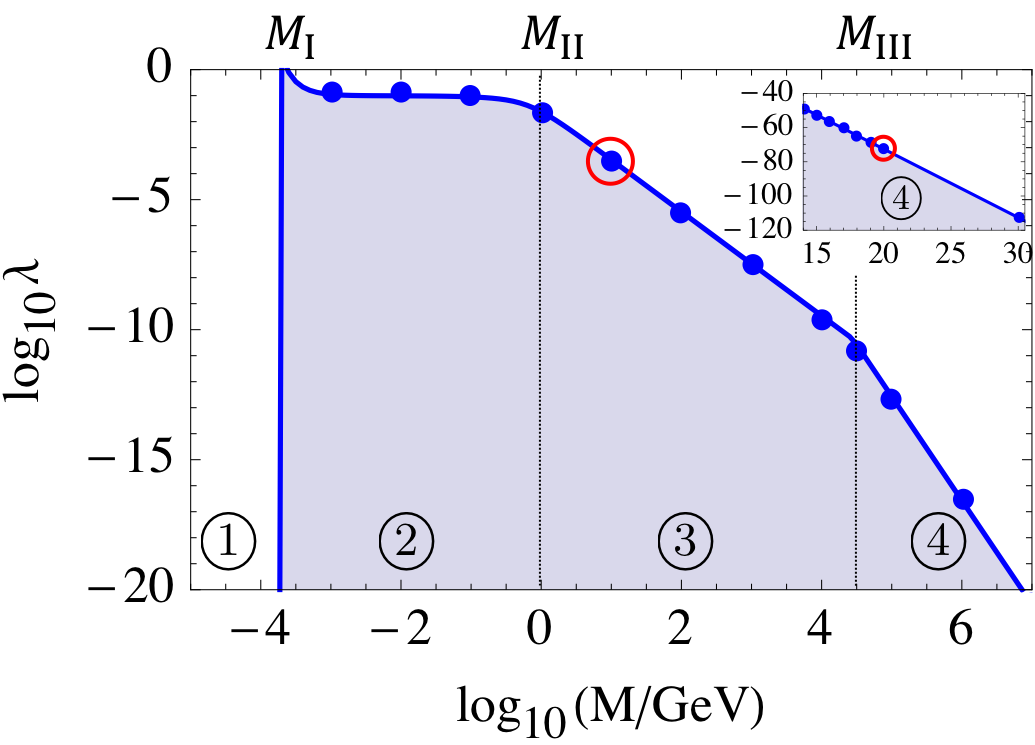
where $\phi_{w}$ is the VEV inside the source mass. There are three values of $M$ that are of particular importance for the exclusion region of a given $\mu$, as illustrated in Fig. 3. First, when $M<\sqrt{\rho_{o}}/\mu\equiv M_{\text{I}}$ (Region \small1⃝), the symmetry is restored in vacuum ($\phi_{o}=0$) such that there is no symmetron force and the parameters are unbounded. Second, when $M_{\text{I}}<M<M_{\text{II}}$ (Region \small2⃝), where $m_{N}R_{N}=1$ is satisfied at $M=M_{\text{II}}\simeq\sqrt{\rho_{N}}R_{N}$, the nucleus is screened with $\lambda_{A}\propto M^{2}$ [Eq. (9)]. Combining with the above discussed acceleration dependence of $a_{s}\propto\phi\nabla\phi/M^{2}\sim\mu^{2}/\lambda M^{2}$, the symmetron acceleration measured by an atom is in fact independent of $M$ in Region \small2⃝: $a_{s}=-\lambda_{A}\phi\nabla\phi/M^{2}\sim\mu^{2}/\lambda$. For $M>M_{\text{II}}$ (Region \small3⃝), $\lambda_{A}\simeq 1$ and $a_{s}\sim\mu^{2}/\lambda M^{2}$, as argued in Ref. BerkeleyNaturePhys and summarized earlier. A fixed $a_{s}$ results in $\lambda\propto M^{-2}$ for a given $\mu$. Third, when $M\geq\sqrt{\rho_{w}}/\mu\equiv M_{\text{III}}$ (Region \small4⃝), where $\rho_{w}$ is the density of the source mass or the vacuum chamber, all materials in the experiment are unscreened [Eq. (2)]. While this region was considered unconstrainable burrage2018tests; BerkeleyNaturePhys, we find that the symmetron force is present albeit suppressed. When unscreened, $\rho<\rho_{*}$, and $\phi_{e}^{2}=\frac{\mu^{2}}{\lambda}\left(1-\frac{\rho}{\rho_{*}}\right)$ [Eq. (2)], such that

Thus, for a fixed $a_{s}$ at a given $\mu$, $\lambda\propto M^{-4}$ in Region \small4⃝.

In short, for a given $\mu$, the symmetron acceleration $a_{s}\simeq-\lambda_{A}\phi_{o}(\phi_{o}-\phi_{w})/M^{2}$ is the same when: $\lambda$ unbounded for $M<M_{\text{I}}$ (Region \small1⃝); $\lambda\propto M^{0}$ for $M_{\text{I}}<M<M_{\text{II}}$ (Region \small2⃝); $\lambda\propto M^{-2}$ for $M_{\text{II}}<M<M_{\text{III}}$ (Region \small3⃝); and $\lambda\propto M^{-4}$ for $M_{\text{III}}<M$ (Region \small4⃝). Figure 3 shows a comparison of simulation results and the above expression for $\mu=10^{-4}$ eV, where Regions \small1⃝-\small3⃝ agree with previous publications BerkeleyNaturePhys; burrage2016constraining while Region \small4⃝ is new result from this study. To have a quantitative comparison, Eq. (12) is fit for an overall scaling factor and $M_{\text{III}}$ with two simulation data points (circled in Fig. 3) at $M=10^{20}$ GeV and $M=10$ GeV where $\lambda_{A}\simeq 1$ for both $M$ values. $M_{\text{I}}$ and $M_{\text{II}}$ are determined solely by the vacuum density $\rho_{o}$ and properties of Cs nucleus. Clearly, Eq. (12) describes the boundary of the exclusion region very well using only two simulation runs. Both the simulation and the theoretical estimate [Eq. (12)] support that the exclusion of $M$ goes well beyond $M_{\text{III}}$ set by the source mass ¹¹ 1 The characteristic density $\rho_{w}$ corresponding to the fitted $M_{\text{III}}$ for $\mu=10^{-4}$ eV (Fig. 3) is about 1.8 g/cm³, which is smaller than the density of the source mass (19.3 g/cm³) and the density of the shell (7 g/cm³), suggesting that the system is unscreened at lower $M$ than that determined by the material density. It is understood that the symmetron field can tunnel through the wall of finite thickness when the material is nearly unscreened. Nevertheless, the difference in $\log_{10}M_{\text{III}}$ is only 0.5 between 1.8 g/cm³ and 19.3 g/cm³, which is negligible compared to the span of $M$ under discussion. , and the validity of $\lambda\sim M^{-4}$ is currently verified up to the simulation capability at about $M=10^{30}$ GeV. Note that the smooth transition between Regions shows that different rescaling of Eq. (1) for numerical simulation are consistent and that the exact distinction between rescaling methods is not critical.

The simulation is extended to other values of $\mu$. At $M=10^{20}$ GeV, $\mu$-$\lambda$ dependence is established, as shown in Fig. 4. We find the data are well described by $\lambda\sim\mu^{2}e^{-\sqrt{2}\mu r_{*}}$, where $r_{*}$ is a characteristic length scale. This relation is in agreement with the two spherical body scenario described by Eq. (5), where $m_{o}\simeq\sqrt{2}\mu$ when $M$ is large [Eq. (3)]. Particularly, the fit of $r_{*}\simeq 1$ cm is indeed the distance of the atoms to the source mass. This geometrical dependence is not captured in Eq. (12), which is motivated from the local field perspective [Eq. (4)]. Thus, a more precise estimate of the symmetron acceleration in the experiment is

where $r_{*}$ is to be determined by fitting the $\mu$-$\lambda$ dependence at large $M$. The introduction of the additional $m_{o}$ dependence yields the sharp increase near $M_{\text{I}}$ in Fig. 3, which will be discussed later in the section.

In Regions \small2⃝ and \small3⃝ where the symmetry is restored in the walls ($\phi_{w}=0$), another constraint exists. Consider the field inside a thick spherical shell of inner radius $R_{w}$, where $\phi=\phi_{w}=0$ inside the sufficiently thick wall. Deviating from the trivial solution of universal $\phi=0$, a perturbative field $\delta\phi$ satisfies (from Eq. (1))

and the boundary conditions for the radial component in the spherical coordinates are $\partial_{r}\delta\phi=0$ at the origin and $\delta\phi=0$ at $r=R_{w}$. The solution is an even-order spherical Bessel function $j_{n}(\sqrt{\lambda}\phi_{o}r)$, and $j_{n}(\sqrt{\lambda}\phi_{o}R_{w})=0$. The lowest allowed $\sqrt{\lambda}\phi_{o}$ is $\sqrt{\lambda}\phi_{o}R_{w}=\pi$, or equivalently $\mu\gtrsim\pi/R_{w}\equiv\mu_{w}$ ($\mu_{w}\simeq 10^{-5}$ eV for $R_{w}=6.1$ cm). In other words, for $\mu<\mu_{w}$ the symmetron field is zero inside the shell and no symmetron force. For $\mu\geq\mu_{w}$, the symmetron field is not zero if the field outside the shell is not zero, i.e., $\phi_{\text{air}}>0$ or equivalently $M>\sqrt{\rho_{\text{air}}}/\mu\equiv M_{\text{III}}^{*}$. In this case, since the field is not separated by the wall, it is in the domain of Region \small4⃝. With a small source mass inside the shell as in the real experiment, $\mu_{w}$ will change slightly and the transition from zero to nonvanishing field will be smooth.

Note that the attempt to establish acceleration scaling versus $(\lambda,\mu,M)$ is also reported in Ref. upadhye2013symmetron and Ref. sabulsky2018experiment, in addition to Ref. BerkeleyNaturePhys. Ref. upadhye2013symmetron uses the one-dimensional plane-parallel (1Dpp) approximation for the symmetron field between two parallel plates, and Ref. sabulsky2018experiment introduces a fitting factor of order 1 to extend the 1Dpp approximation to the interior of a vacuum chamber. Equation (14), on the contrary, is applicable to a wide range of $(\lambda,\mu,M)$ with fixed geometric parameters. It also allows exclusion in Region \small4⃝.

To summarize, the constraints of symmetron parameters $(\lambda,\mu,M)$ are characterized by several bounds associated with experimental parameters, as depicted in Fig. 5. $M_{\text{I}}=\sqrt{\rho_{o}}/\mu$, below which the symmetry of the field is restored in vacuum and the field is zero everywhere. $M_{\text{II}}=\sqrt{\rho_{N}}R_{N}$, below which the nucleus of the atomic test particle is screened with a screening factor $\lambda_{A}\propto M^{-2}$. $M_{\text{III}}=\sqrt{\rho_{w}}/\mu$, below which the symmetry is restored in the vacuum chamber walls, and above which the whole system is unscreened. $M_{\text{III}}^{*}=\sqrt{\rho_{\text{air}}}/\mu$, below which the symmetry is restored in air and $\phi_{\text{air}}=0$. $\mu_{w}=\pi/R_{w}$, below which the field is zero inside the enclosure if the field outside is zero. $\mu_{*}\sim 280/r_{*}$, at which the field is about $e^{-400}$ of its peak value for a given $M$.

The procedure for finding the exclusion region for a specific experimental symmetron acceleration upper bound is as follows. First, determine the characteristic length scale $r_{*}$. It can be found by fitting simulation results at large $M$ for different $\mu$, as in Fig. 4, where the screening factor is essentially 1 and the system is unscreened. Or, one can take the approximate distance of the atomic cloud to the source mass as $r_{*}$. Second, identify the densities of vacuum $\rho_{o}$, the wall $\rho_{w}$, the ambient air $\rho_{\text{air}}$, and the nuclear properties $\rho_{N},R_{N}$. Third, identify the characteristic size of the enclosed vacuum $R_{w}$. Finally, based on the simulation result of one parameter set $(\lambda,\mu,M)$, apply the $M$-$\lambda$ scaling rules in Regions \small1⃝-\small4⃝ and $\lambda\sim\mu^{2}e^{-\sqrt{2}\mu r_{*}}$ for fixed $M$ [or equivalently Eq. (14)] while respecting the bounds of $M_{\text{III}}^{*}$ and $\mu_{w}$ laid out in Fig. 5. Figure 6 shows the comparison of simulation results at various $(\lambda,\mu,M)$ versus the region described by the above procedure, which is a realization of Eq. (14) with modifications imposed by $\mu_{w}$ and $M_{\text{III}}^{*}$. Clearly the simulation results reside on the surface defined by the recipe except very near the edges of $\mu_{w}$ and of $M_{\text{III}}^{*}$. Note that there is a lip around $\mu\sim 10^{-2}$ eV in the surface plot of the exclusion region, which corresponds to the sharp increase of $\lambda$ near $\log_{10}(\mu/\text{eV})=-4$ in Fig. 3. It is because $m_{o}\sim 0$ when $M\gtrsim M_{\text{I}}$ ($\rho_{o}\lesssim\rho_{*}$) such that the exponential factor of $e^{-m_{0}r_{*}}$ in Eq. (14) approaches unity and that the sensitivity is recovered in a narrow range of $M$ bounded by the $m_{o}^{2}$ factor.

Constraints on symmetron theory have also been established through astrophysical observations. By comparing distances of remote stars estimated from methods either sensitive or insensitive to the screening mechanism, bounds on the screening effect and thus on the theories are obtained burrage2018tests; sakstein2017tests; jain2013astrophysical; vikram2014astrophysical. Prior to this work, the constraints from analyzing laboratory experiments in atomic physics are far away from the astrophysical bounds in the parameter space. Thanks to the discovery of Region \small4⃝ from laboratory symmetron acceleration measurements, we are able to extend the atomic physics constraints by more than 20 orders of magnitude to overlap with those from the astrophysical observations where $M$ is of the magnitude of $10^{15}$ GeV or higher. Figure 7 shows simulation results (dots) for $\mu=10^{-4}$ eV, with the range of $M$ extended to $10^{30}$ GeV. Also shown in the figure is the bound calculated based on Eq. (14). Atomic exclusion of $\lambda$ is the shaded area under the bound. The astrophysical constraint, shown in yellow, is reproduced from Ref. burrage2018tests. As shown in Fig. 7, not only the predicted dependence of Eq. (14) but also simulation results make direct comparison in the parameter regions relevant to astrophysics.

One may argue that since all materials in the experiment are unscreened ($\rho<\rho_{*}$) in Region \small4⃝ (see Sec. III.4), a detailed modeling of the environment including the optical table, the floor and ceiling of the building is required for a reliable simulation. In fact, the Compton wavelength of the symmetron field at $\mu=10^{-4}$ eV is $m_{s}^{-1}=2^{-1/2}\mu^{-1}(1-\rho/\rho_{*})^{-1/2}\simeq 2^{-1/2}\mu^{-1}\simeq 1.4$ mm, which is short compared to distances of surrounding objects to the experiment. Thus, the symmetron field in air reaches the VEV around the experiment, effectively isolates the experiment from its environment. This phenomenon is evident in Fig. 7(b), where the symmetron field settles to $\phi_{e}$ of the air, in a short distance. The validity of the simulation result is thus based on a reasonable assumption that the experimental apparatus of Ref. BerkeleyNaturePhys is mostly surrounded by a layer air of at least 2 cm, and that supporting structures to the apparatus would only mildly modify the field inside the vacuum chamber.

The astrophysical constraint is about 10 orders of magnitude more stringent than the current atomic physics constraint for $M>10^{15}$ GeV, though the dependence on $\mu$ is not elaborated. The similarity of $M$-$\lambda$ dependence is a validation of both approaches. While new astrophysical data or analysis could improve the constraint further, specifically designed atom interferometer experiments may provide definite enhancements in near future.

It is also interesting to note that in Region \small4⃝ all materials are unscreened, so that the advantage of using atoms may not be significant as in other regions. Reanalysis of results using macroscopic test objects, as was done in Ref. upadhye2013symmetron, may provide a better bound than atomic tests here after addressing potential practical systematics.