Parallel Randomized Algorithm for Chance Constrained Program

Randomized optimization can be used to solve program in (1). The flow diagram of randomized optimization applied for chance constrained program is illustrated in Fig. 2. Firslty, decision samples are randomly extracted from $\mathscr{U}$ which might not satisfy the chance constraints. Thus, in the next step, violation probability of extracted samples are verified and the unqualified samples are discarded. The optimizer are chosen from the qualified samples. The process is repeated until termination criterion is satisfied and optimizer is outputted finally.

Randomized optimization algorithm is numerical optimization algorithm which does not require the gradient of the problem and it can therefore be used on functions that are not continuous or differentiable[11]. Moreover, if the problem is constrained and the constraints might be non-convex, randomized optimization algorithm still ensures the convergence to the optimizer [12]. Random optimization moves to better positions iteratively in the exploration domain (the exploration domain should be a subset of feasible domain), sampling near the current position according to normal distribution or uniform distribution[13].

Let $F:\mathscr{V}\subset\mathbb{R}^{n}\rightarrow\mathbb{R}$ be the cost function to be minimized in the feasible domain $\mathscr{V}$. Let $v\in\mathscr{V}$ denote a position or candidate optimizer in the feasible domain. The typical randomized optimization algorithm can then be denoted as algorithm 1 and expressed as following[14]:

• •

  Step 1: Initialize $v\in\mathscr{V}$ randomly
  

• •

  Step 2: Extract new sample $v^{\prime}\in\mathscr{V}_{v}$ obeying uniform distribution or normal distribution. Here, $\mathscr{V}_{v}$ is a neighbour of $v$, for instance, as $\mathscr{V}_{v}=\{v_{f}\in\mathscr{V}|\left\|v_{f}-v\right\|^{2}<\epsilon_{v}\}$
  

• •

  Step 3: If $F(v^{\prime})<F(v)$, set $v=v^{\prime}$
  

• •

  Step 4: Examine whether the termination criterion is met(e.g. number of iterations), if termination criterion is met, go to Step 5, otherwise, go to Step 2 and repeat
  

• •

  Step 5: Set $v$ as optimizer

The proposed optimizer exploration algorithm firstly extracts $N_{u}$ samples, $\{u_{1},...,u_{N_{u}}\}\in\mathscr{U}$ , from the decision domain. However, not all the samples satisfy the chance constraints. The violation probabilities of decision samples should be validated. Violation probability of decision $u$ is denoted as

For given decision $u_{i}$ and disturbance $\delta_{k}$, a boolean function can be denoted as

If $N_{\delta}$ samples, $\{\delta_{1},...,\delta_{N_{\delta}}\}$, are extracted from $\Delta$ independently obeying the identical distribution, the estimate violation probability can be written as

According to law of larger numbers, as $N_{\delta}\rightarrow\infty$, $\hat{V}(u_{i})$ converges to $V(u_{i})$ with probability one[15]. Furthermore, for fixed sample number $N_{\delta}$, the mean value of $\hat{V}(u_{i})$, denoted as $\mathbb{E}\{\hat{V}(u_{i})\}$, equals to $V(u_{i})$ and the variance $\sigma\{\hat{V}(u_{i})\}$ equals to $\frac{\sigma\{V(u_{i})\}}{N_{\delta}^{2}}$. Therefore, based on the above disturbance sampling, $V(u_{i})=Pr\{h(u_{i},\delta)>0\},\forall i\in\{1,...,N_{u}\}$ can be calculated and the ones with violation probability larger than $\alpha-\alpha_{\epsilon}$ are discarded, where $\alpha_{\epsilon}$ is within $(0,\alpha)$. The boundary for discarding samples is chosen slightly smaller than the required one for a techinical consideration. Since the estimate $\hat{V}(u_{i})$ is centered at $V(u_{i})$ with variance, half of the estimates might be located in the position where the real violation probability is larger than the required one. By chosen a slightly smaller bound, the percentage of points located out of feasible area decreases as $N_{\delta}$ increases. The remained feasible samples are used to calculate the corresponding cost function values. The one with minimal cost value is chosen and compared with the current optimizer. If it is better than the current optimizer, it will be regarded as optimizer instead. The above steps are repeated until termination criterion is met, for instance, number of iterations. The algorithm for exploring the feasible optimizer is summarized in Algorithm 2

• •

  Step 1: Initialize optimizer $u_{f}^{*}\in\mathscr{U}$ randomly
  

• •

  Step 2: Extract $\{u_{1},,...,u_{i},...,u_{N_{u}}\}\in\mathscr{U}$
  

• •

  Step 3: Extract $\{\delta_{1},...,\delta_{N_{\delta}}\}\in\Delta$ randomly
  

• •

  Step 4: Calculate approximately $V(u_{i}),\forall i\in\{1,...,N_{u}\}$ according to Eq. (8) and (9), discard all $u_{d}$ that $V(u_{d})>\alpha-\alpha_{\epsilon}$, and the remained solution set is $\mathbb{U}_{f}$
  

• •

  Step 5: If $\mathbb{U}_{f}=\emptyset$, return to Step 1, else if $\mathbb{U}_{f}\neq\emptyset$, go to Step 6
  

• •

  Step 6: Set optimizer as $u^{*}=\underset{u\in\mathbb{U}_{f}}{\text{argmin}}J(u)$
  

• •

  Step 7: Replace optimizer $u_{f}^{*}=u^{*}$ and go to Step 8 if $J(u^{*})<J(u_{f}^{*})$; Return to Step 2 directly if $J(u^{*})\geq J(u_{f}^{*})$
  

• •

  Step 8: Examine whether the termination criterion is met (e.g. number of iterations), if termination criterion is met, go to Step 6, otherwise, go to Step 1 and repeat
  

• •

  Step 9: Set $u_{f}^{*}$ as optimizer.

Moreover, the above algorithm is briefly illustrated in Fig. 3 as well. Apparently, the algorithm is parallel compared to the original randomized algorithm. It is able to applied in the hardware which supports parallel algorithm and can improve computation efficiency.

The targeted problem in the numerical simulation is a non-convex program with chance constraints. The decision domain is $\mathscr{U}=[-6,5]^{2}$. The cost function is

The constrained function is

where $a_{1}=1.5,a_{2}=2,b_{1}=2,b_{2}=3$, $\delta$ is random variable which obeys normal distribution $\mathscr{N}(0,1)$. Moreover, the violation probability level is $\alpha=0.05$.

The proposed method is applied to solve the targeted problem, comparing with scenario approach presented in [7]. In scenario approach, independent samples $\delta^{(i)},i=1,...,N$ is identically extracted from $\Delta$ randomly, a deterministic convex optimization problem can be formed as

which is a standard finitely constrained optimization problem. The optimal solution $\hat{u}_{N}$ of the program Eq. (12) is called as the scenario solution for program Eq. (1) generally. Moreover, since the extractions $\delta^{(i)},i=1,...,N$ is randomly chosen, the optimal solution $\hat{u}_{N}$ is random variable. If $\hat{u}_{N}$ is expected to satisfy

then, $N$ should have a lower limitation $N_{l}$

Note that $\beta$ is an important factor and choosing $\beta=0$ makes $N_{l}=\infty$. Namely, if the number of chosen samples gets larger, the probability of satisfying the original chance constraints approaches 1. Actually, when number of chosen samples becomes infinity, the samples cover the whole sample space, not only the feasible area determined by chance constraints, it becomes totally robust.

The results of optimizer exploration are presented here. In this numerical simulation, both proposed method and scenario approach are used to solve the targeted problem. The numerical simulation adopts Monte Carlo methodology, namely, the procedure of exploring the optimizers is repeated for a large number of times and the samples of $u$ and $\delta$ are extracted obeying the identical distribution in every simulation time. 500 times of simulation were done in this validation. Moreover, for the proposed method, the parameter $\alpha_{\epsilon}$ is chosen as 0.005.

In Fig. 4, evolutions of the solution during computation process for proposed method are plotted, for both cases $N(\delta)=100$ and $N(\delta)=1000$. In every simulation, the solutions converge to the small intervals for both $u_{1}$ and $u_{2}$. The final converged values of decision are plotted in Fig. 5. Green star marks stand for solutions from proposed method using 100 disturbance samples, blue points are solutions from proposed method using 1000 disturbance samples, magenta squares are solutions from scenario approach using 100 disturbance samples and red circles present the solutions from scenario approach using 1000 disturbance samples. Apparently, proposed method can converges to the $5\%$ boundary where the cost is minimal in the probabilistic domain. However, for scenario approach, the solution cannot converge to the boundary. In every simulation, the sampled $\delta$ are different, the constraints of problem expressed by Eq. (12) are different, the solution are therefore different and distributed in a larger area. When $N(\delta)$ is small, the considered deterministic constraints are not enough to ensure the violation probability, the solutions are mostly distributed outside the feasible area as shown by magenta squares in Fig. 5. While, as $N(\delta)$ gets larger, the constraints become more and the solutions are consequently conservative and distributed inside the boundary as red circles in Fig. 5.

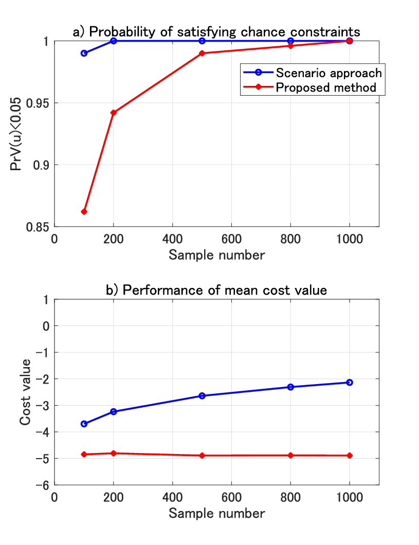
Furthermore, Fig. 6 shows the statistical results of cost values and violation probabilities in all simulations. From these results, obviously, the proposed method achieves the trade-off between violation probability and optimization in a more stable way. While, scenario approach fails to find the balance. It gets minimal cost with loss of violation probability performance in less disturbance samples’ simulations. On the other hand, it provides too conservative results on violation probability with worse cost performance. The mean costs of the proposed method are all near the boundary even the samples of disturbance become more. The violation of chance constraints becomes less when there are larger sample numbers of disturbance.

References

- [1] A. Prekopa, On probabilistic constrained programming. in Proceedings of the Princeton Symposium on Mathematical Programming, Princeton University Press, Princeton, NJ, pages 113–138. 1970.
- [2] A. Charnes, and W. W. Cooper, Chance constrained programming. Management Science, volume 6, no. 1, pages 73-79. 1959.
- [3] X. Shen, and T. Shen, Chance-Constrained Optimization for Torque Tracking Control with Improving Fuel Economy in Spark-Ignition Engines. SICE Journal of Control, Measurement, and System Integration, volume 11, no. 4, pages 365-371. 2018.
- [4] M. C. Campi, and S. Garatti, Introduction to the scenario approach, MOS-SIAM Series on Optimization, Philadelphia, 2019.
- [5] G. Calariore, and M. C. Campi, The scenario approach torobust control design. IEEE Trans. Automatic Control, volume 51, no. 5, pages 742-753. 2006.
- [6] J. Luedtke, and S. Ahmed, A Sample Approximation Approach for Optimization with Probabilistic Constraints. SIAM Journal on Optimization, volume 19, no. 2, pages 674-699. 2008.
- [7] M. C. Campi, and S. Garatti, A sampling-and-discarding approach to chance-constrained optimization: feasibility and optimality. Journal of Optimization Theory and Applications , volume 148, no. 2, pages 257–280. 2011.
- [8] M. Cannon, Chance-constrained optimization with tight confidence bounds. arXiv:1711.03747 [math.OC], 2018, arXiv:1711.03747.
- [9] R. B. Gramacy, and H. K. H. Lee, Optimization Under Unknown Constraints. arXiv:1004.4027 [stat.ME], Jul. 2010, arXiv:1004.4027.
- [10] V. Picheny, R. B. Gramacy, S. M. Wild, and S. Le Digabel, Bayesian optimization under mixed constraints with a slack-variable augmented Lagrangian. arXiv:1605.09466 [stat.CO], 2016, arXiv:1605.09466.
- [11] J. Matyas, Random Optimization. Automation and Remote Control, volume 26, no. 2, pages 246-253. 1965.
- [12] N. Baba, Convergence of a random optimization method for constrained optimization problems. Journal of Optimization Theory and Applications, volume 33, no. 4, pages 451-461. 1981.
- [13] C. C. Y. Dorea, Expected number of steps of a random optimization method. Journal of Optimization Theory and Applications, volume 39, no. 2, pages 165-171. 1983.
- [14] F. J. Solis, and R. J. B. Wets, Minimization by Random Search Techniques. Mathematics of operations research, volume 6, no. 1, pages 19-30. 1981.
- [15] W. Feller, An introduction to probability theory and its applications, John Wiley and Sons, Inc., 1968.