Option-based Equity Risk Premiums
Abstract
We construct the term structure of the (forward-looking, US market) equity risk premium from SPX option chains. The method is “model-light”. Risk-neutral probability densities are estimated by fitting -component Gaussian mixture models to option quotes, where is a small integer (here 4 or 5). These densities are transformed to their real-world equivalents by exponential tilting with a single parameter: the Coefficient of Relative Risk Aversion . From history, I estimate . From the inferred real-world densities, the equity risk premium is readily calculated. Three term structures serve as examples.
1 Introduction and summary
The equity risk premium (ERP throughout) has frequently been called the most important number in finance. To be fair, so have LIBOR and the 10-year US Treasury yield. It’s certainly the elusive one: interest rates are readily observed, while the ERP (as defined here) is a forward-looking “market” expectation, requiring estimation.
US market history suggests a long-run (unconditional) ERP of 4-6% per year. Our topic is the difficult problem of estimating time variation and term structure effects. Plausibly, key drivers of this conditional ERP are outlooks for inflation, rates and yields, earnings, and volatility.
There are many models and approaches in the literature. An interesting and diverse collection of views is found in Hammond et al. (2011). In Duarte & Rosa (2015), the authors use the best linear combination of 20 models to produce, among other things, ERP term structure estimates at various dates. In agreement with them, we find that the ERP term structure has significant time variation and can be flat, upward, or downward sloping. Later, in Sec. 5.3, we further compare our results to theirs.
Many authors use time series models to infer an ERP from the (weak) predictive power of financial ratios: dividend yields or PE ratios. However, there is controversy over the predictive power. Even without the controversy, a difficulty is that financial ratios don’t vary much in the short-term. Another difficulty: beyond key drivers is the large and nebulous set , the time ‘‘state-of-the-world” -- any element of which may become (momentarily) important to the market’s outlook. For example, at this writing, trade negotiations have become a market focus.11 1 Update: at this revision, the COVID-19 pandemic is driving everything. Using the methods here, the US ERP during the pandemic is studied in Lewis (2020).
Here, we develop a new approach, using SPX options and a one-parameter change-of-measure to estimate the ERP term structure at arbitrary trade dates. It’s relatively objective, driven largely by forward-looking market data: option quotes.
While certainly not “model-free”, I call it “model-light”. No stochastic process is adopted for SPX. No financial ratios are singled out as explicit drivers of the ERP, although they can certainly play an implicit role in market expectations. Indeed, anything the market deems momentarily important to its outlook, as long as it’s reflected in the options market, can influence our ERP estimates. Our key modelling assumption – which has theoretical and historical support – is that an exponential change-of-measure transforms the option-based risk-neutral density (RND) to the real-world density (RWD).
Figs. 2-4 show three examples of our new ERP term structure estimates. Near expirations are closely spaced in time, and made more visible with log time scales. The trade dates shown have relatively high, low, and middle-of-the-road (recent) volatility environments, as measured by the VIX index: see Fig.1. In the higher volatility environment, the ERP estimates decay from a large value (from 2-day options) toward the longer-run averages (from 2.5 year options). Conversely, in the lower volatility environment, the ERP term structure is increasing with the term, again toward unconditional values. Finally, the last volatility environment yields a relatively flat term structure. Qualitatively, those are plausible term structure behaviors, key drivers here being volatility and risk-aversion. The decay from 26% is just a recent example. More generally, volatility and the short-term (annualized) ERP estimates can be expected to be very high in systematically stressed markets – let’s say with VIX above 40 – as was seen in the Financial Crisis of 2007-2008.
The figure ERP bands use a Coefficient of Relative Risk Aversion, , in the range , with being the central estimate (central curve). We argue for that range in Sec. 2, using market history. Note that also serves as the parameter for the exponential change-of-measure. Theoretically, the exponential form follows from a standard equilibrium market-clearing argument using a representative investor with power utility – an argument reviewed in the Appendix. To estimate , we use the fact that it is the exponential tilt parameter that turns a (long-run historical) excess return sequence into a zero-mean sequence: see eqn (12) below. Looking forward with options data (in Sec. 4), we estimate RND’s by fitting SPX option quotes to Gaussian mixture models. Then, effects a one-parameter change of measure from the RND’s to RWD’s, the real-world probability densities. Examples are shown in Figs. 10-12. Given the RWD’s, the ERP’s are readily calculated. That’s the paper in a nutshell.
For the remainder of this section, I give a more elaborated summary. Key formulas are boxed.
1.1 Some definitions and notations
What exactly do we mean by the ERP? There are many closely related definitions. First of all, we adopt a US perspective, so “equities” means a broad-based (capitalization weighted) measure of the entire US equity market, frequently proxied by the S&P 500 Index. Second, the ERP is far from a single number. Like interest rates, it’s time-varying, with a time-varying term structure. With denoting a (real-world) expectation conditional on date- information – broadly speaking: the “state of the world” – we define:
| (1) |
- •
is a future random total return on the equity market from to , and
- •
is a time- observable risk-free return (using US Treasury instruments).
Returns in (1) are simple total returns: , where is a total-return index incorporating reinvested dividends. (Without a bar, is the price series without dividends). Call the excess total return. Like interest rates, we’ll always give estimated ERP’s on an annualized percentage basis. For those, we multiply the ERP calculated from (1) by , where the annualization factor , with time measured in years. That convention is used in Figs. 2-4 and associated tables.
Let’s call the risk-free basis for the ERP. There are two natural choices in the literature for the risk-free basis. One choice ignores the and use a short-maturity US Treasury bill return for each basis. The second choice, which we employ, uses the time- return available from Treasury instruments that mature at . That’s more natural for our forward-looking, option-based estimates, and is used in Figs. 2-4. For our history-based estimates of , is a realized return. Those are constructed from monthly Tbill returns (when is one month), chaining together monthly returns (when is greater than a month), or pro-rating monthly returns (when is one day).
| Reference | Description |
|---|---|
| Bliss & Panigirtzoglou (2004) | Smoothing spline fit to mid-quote IV’s flat (Gaussian) extensions |
| Gatheral & Jacquier (2013) | 5-parameter SVI fit to mid-quote IV’s implies a full RND |
| Fengler (2005) | Smoothing spline fit to option prices implies a partial RND |
| Figlewski (2010) | Weighted spline fit to mid-quote IV’s + GEV distribution extensions |
| Malz (2014) | Interpolating spline fit to mid-quote IV’s flat (Gaussian) extensions |
1.2 Estimating risk-neutral and real-world probability densities
Let , denote the time- RND for , where is the terminal index price. The RND depends upon , the starting index price, and generally , our catch-all for information known at . These latter dependencies are freely suppressed, but implied by the subscript in .
From Treasury rates, infer deterministic risk-free discount factors , using various of our notations. Then, where is the option strike price, call option values are given by
| (2) |
where . Given a set of option prices, , there are various types of approaches to estimating :
- (1)
Modelling the underlying stock process.
- (2)
Fitting approaches suggested by the Breeden-Litzenberger relation.
- (3)
Direct modelling of the ℚ-density or (as here) the pdf for .
Type 1. A typical framework is the following. Postulate a (continuous-time) ℚ-measure jump-diffusion process, , where is a parametrized stochastic volatility process and is a parametrized (zero-mean) jump process. Free parameters are estimated by fits to option prices, implied volatilities, or similar targets. Parameters estimates yield ’s.
The main problem is that stationary models will have, let’s say, 6-12 parameters for computational tractability. Unfortunately, such a small number will prove wholly inadequate for fitting a large option data set with multiple trade dates. One could adopt (large) parameter sets that vary with the trade date and option expiration , but this does not typically result in a logically consistent stochastic process. For example, why should the putative underlying process even know about the arbitrary dates of option expirations?
Type 2. If calls were marketed with a continuum of strikes , and zero bid-ask spreads, then the Breeden-Litzenberger relation,
| (3) |
would yield a unique, completely “model-free” risk-neutral density. Then, given discrete strikes and positive spreads, use interpolating or smoothing splines to fit option prices or implied volatilities (IV’s for short). Generally, it’s better to fit the , which yields a smooth function . From that, a smooth option pricing function is available, where is the Black-Scholes formula, suppressing other arguments. Finally, (3) and the chain rule for differentiation yield the estimated .
In my opinion, the main issue with this type of approach is deciding how to extrapolate the to the ranges and . Here represent the range of marketable strikes. You must extrapolate to find a proper (norm=1) RND. It’s difficult to devise an extrapolation method that doesn’t feel ad hoc. Some references for this type of approach are given in Table 1.
Type 3. Here, one parameterizes directly the RND. After some experimentation with type 2 methods, I ultimately adopted a type 3 method. Specifically, with log price-returns , the corresponding RND is . Then, I fit a Gaussian Mixture Model (GMM) to option quotes.22 2 My thanks to Thijs van den Berg, who suggested exploring GMM’s. Prior to that suggestion, I was fitting smoothing splines to IV’s (similar to some Table 1 methods) and attempting extrapolation. But I quickly converted to the GMM approach described here: it seemed a ‘natural’ for my ERP problem setup. The mixture consists of Gaussians:
| (4) |
where , and is a small integer (4-5 in my fits).
(Notations: strictly, I should write instead of , but I don’t for notational simplicity. Also, I move to small letters for log-arguments).
The fitted parameters are positive weights, , and drifts and volatilities, . After a normalization and martingale condition, this leaves free parameters at each pair associated to a trade date and an option expiration. Using (2) and the corresponding put value formula, free parameters are adjusted to fit option quotes – details are found in Sec. 4.2.
Under an exponential change of measure, (6) below, the RWD will also have Gaussian tails. At first glance, this might give pause because it’s well-known that single Gaussian fits to historical S&P 500 returns are strongly rejected by statistical tests. However, we stress this rejection is irrelevant to fits of mixtures. To see why, consider the analogous RND case. A single Gaussian implies flat IV smiles, a shape which would lead similarly to strong rejection of the proposed density. In contrast, a GMM can nicely fit market smiles, as we will show.
Indeed, as I suggest in footnote 2, in my opinion the GMM method is a ‘natural’ for the ERP problem, at least as set up here. Let me summarize some of the attractive features.
First, the GMM is able to achieve good fits to option quotes.
Second, by modelling a density directly, smile extrapolation is built-in and does not need to be grafted on – as is the case with spline fits to IV’s.
Third, the GMM accommodates arbitrary in the exponential change of measure. A plausible alternative might choose from a class of models with exponential (‘semi-heavy’) tails. For example (although it is actually a type 2 method), J. Gatheral’s SVI method has exponential tails Gatheral & Jacquier (2013). That’s fine, but there will be a restriction on relative to the tail parameters, so that the denominators in (6) below exist. This restriction is certainly not a deal breaker for semi-heavy tails, but adds a complication if you insist on them. Finally, option values and exponential changes of measure are nicely tractable under GMM.
Transforming to log total-return densities. The cost of carry parameters are . How we get them is explained later. Here is the continuously compounded risk-free interest rate and is a continuously compounded dividend yield for the underlying stock index. Given those, we have the index forward price
If the dividends were reinvested into the index, the index would be different: call it . With that one, the forward would be . Given our original index price , this motivates us to associate a random total-return index which incorporates hypothetically reinvested dividends. The associated log total-return is , and the associated risk-neutral density is found by a simple translation:
| (5) |
Transforming to the real-world probability density. Finally, we move from risk-neutral (ℚ-measure) densities to real-world (ℙ-measure) densities using the exponential tilt associated to a risk-averse representative agent model. The agent, with time- wealth , chooses investments with payoffs at by maximizing her expected utility . Here is an impatience parameter that need not be estimated, and is the agent’s Coefficient of Relative Risk Aversion (CRRA). To clear the market, all the agent’s wealth must be optimally invested in the aggregate securities market; thus , the total return equity index from above. While this utility model is well-known in spirit, there are many variations: our version is developed in Appendix A. Using total return pdf’s, it leads to the duality:
| (6) |
1.3 Calculating the ERP
| (7) |
Use (4),(5) and some routine calculations to evaluate (7). The result for the option-based ERP is relatively simple – on an annualized percent basis:
| (8) | ||||
Here the are the GMM fits to option quotes at for expiration .
This concludes our summary.
2 Estimation of the CRRA parameter
There is a large literature on this topic. A classic study is Friend & Blume (1975) who concluded (adapting to our notation):
The empirical results … indicate that the assumption of constant proportional risk aversion for households is a fairly accurate description of the marketplace … The implication is that for the typical household is in excess of 1.0 – contrary to the proportion of the log utility function. Since the market price of risk is probably around 2.0 or more, is more likely to be in excess of two.
Unfortunately, the subsequent literature muddied up this relatively clean picture.33 3 For example, Bliss & Panigirtzoglou (2004) present (their Table VII) literature estimates from eleven studies with estimates ranging from 0-55. Our approach is straightforward and agreeable with Friend & Blume: we estimate . At the end of this section, we compare with the study mentioned in footnote 3.
We begin with the martingale relations.
Martingale relations. In a risk-neutral world, the ERP is zero and (1) reads
| (9) |
for all pairs. Recall , where is a total-return index (i.e., including reinvested dividends). Thus, (9) has the well-known equivalent:
| (10) |
Recall in our previous notation. Thus, (10) says the discounted (total-return) index behaves like a martingale under the risk-neutral measure – the starting point for many dynamical stochastic process models. This justifies calling either (9) or (10) ‘martingale relations’.
The estimator. To estimate , consider where is, for example, one-month. Then employ (9) on an unconditional basis using a long series of historical one-month equity total returns. That is, first write (9) as
| (11) |
Here and is the unconditional density for , the month- log-total-return of the equity aggregate. The are then the monthly Tbill returns. Next, estimate from the empirical density using a list of monthly historical returns from (let’s say) 1926 to date. (We consider other periods also). The empirical density is , using the Dirac delta. Upon substitution in (11): is estimated by , the solution to
| (12) |
In other words, is the exponential tilt parameter that turns the historical equity excess return sequence into a zero-mean sequence. This is ‘dynamics-free’: no specific stochastic process is imposed upon the sequence. Of course, our approach relies upon the assumption that this exponential change of measure is indeed used by the market (or the representative agent if you like). Given the need to either impose dynamics or impose a preference model, the latter choice is the minimal (“model-light”) one.
2.1 Data sources for historical equity returns
I use two equity indices as proxies for the aggregate U.S. equity market:
- (i)
The S&P 500/Composite Index (SBBI);
- (ii)
All US exchange-listed stocks (Fama and French online data from CRSP)
Some additional detail:
S&P 500 Index. The S&P 500 Index has modern
form (close to 500 stocks) starting March 4, 1957. However,
this series is commonly joined with the earlier “S&P Composite” (90 large U.S. stocks),
extending back to 1926 and still called the S&P 500. Our main source for the joined series
was the “SBBI Yearbook: Stocks, Bonds, Bills, and Inflation” Ibbotson & Duff & Phelps (2016). I used
SBBI data for monthly total returns through calendar year 2017 and updated the results
myself through June 2019. For the update (capital appreciation), I used Mathematica’s built-in curated data (FinancialData["SP500"]).
To update the dividend income returns, I used the “S&P 500 Dividend Points Index (SPXDIV)”,
available online at https://us.spindices.com/indices/equity/sp-500-dividend-points-index-quarterly.
There was excellent agreement
among these various sources where they overlapped.
Fama and French data. While SBBI data is monthly, Kenneth French provides (and updates online) a daily series used by him and Eugene Fama in their research. (FF data for short). Specifically, they provide a capitalization weighted, daily excess return on the ‘market’, represented by “all CRSP firms incorporated in the US and listed on the NYSE, AMEX, or NASDAQ that have a CRSP share code of 10 or 11”. CRSP is the Center for Research in Security Prices, part of the Booth School of Business at the University of Chicago. The Ken French data library and further details may be found at https://mba.tuck.dartmouth.edu/pages/faculty/ken.french/data_library.html. The risk-free rate is described as the “Treasury bill rate (from Ibbotson Associates)”, likely the SBBI series prorated to daily returns.
2.2 S&P500 results
Table 2 shows the estimates from the monthly SBBI series using various start dates through June 2019. Also shown are various moments of the true series and the inferred risk-neutral distribution (from tilting at the estimated ). Recall the ‘excess returns’ are the (annualized) series; those have zero -means by construction. Higher moments shown are computed from log-returns: .
Why those starting dates? Jan 1926 starts the entire series. Jan 1950 roughly starts the post-WWII period, often considered a structural break to a world of reduced average volatility and less frequent recessions. Recall Apr 1957 marks the start of the ‘true’ S&P 500 Index. Finally, Jan 1987 and Jan 1988 are convenient starts to show both pre- and post- Oct 19, 1987 data, as the Black Monday market crash is often considered an outlier.
As one sees from Table 2, estimates all lie within a range of . Post-WWII estimates tend to be higher than the entire series. Those are the results from that table important for the ERP.44 4 Some incidental observations. The risk-neutral standard deviations are always larger than the true values – by amounts ranging from roughly 1 to 1.5 vol points (annualized percentage points). Risk-neutral skewness’s are uniformly more negative than real-world. Kurtoses are smaller post-WWII and have similar risk-neutral and real-world values for every start date.
Various start dates through June 2019. Monthly observations. Means and Std Dev’s are annualized and in percent. For example, ‘Mean excess returns’ are (avg monthly total returns less monthly Tbill returns). Standard deviations, skewness, and kurtosis are based upon continuously compounded total returns (log-returns). ‘True’ = actual: realized. ‘RN’= risk-neutral: the exponentially-tilted empirical -distribution with tilt parameter .
| Mean | ||||||||||
|---|---|---|---|---|---|---|---|---|---|---|
| Start | Excess Return | Std Dev | Skewness | Kurtosis | ||||||
| month | True | RN | True | RN | True | RN | True | RN | ||
| Jan 1926 | 1122 | 2.28 | 8.14 | 0 | 18.6 | 19.7 | -0.50 | -1.29 | 11.0 | 10.4 |
| Jan 1950 | 834 | 3.58 | 7.73 | 0 | 14.3 | 15.2 | -0.67 | -0.95 | 5.5 | 6.3 |
| Apr 1957 | 747 | 2.96 | 6.52 | 0 | 14.5 | 15.3 | -0.69 | -0.93 | 5.6 | 6.2 |
| Jan 1987 | 390 | 3.33 | 8.04 | 0 | 15.0 | 16.5 | -1.09 | -1.36 | 6.7 | 7.4 |
| Jan 1988 | 378 | 3.83 | 8.15 | 0 | 14.2 | 15.2 | -0.78 | -0.90 | 4.7 | 4.8 |
2.3 Temporal aggregation of the S&P500 data
Strictly speaking, the stock market never offers a stationary ‘return generating process’, in the sense of a well-specified casino game. Nevertheless, if the risk-aversion model is not too far off the mark, given long ‘pseudo-stationary’ samples, one would expect similar estimates regardless of the return observation frequency: daily, monthly, quarterly, and so on. Given our monthly S&P 500 total returns, we aggregate the data into longer periods and repeat the estimating procedure.
Results. In Table 3 we show the effect of this temporal aggregation, using the longest SBBI data period: Jan 1926 – June 2019. When aggregating, there are two choices: overlapping or non-overlapping periods. We show both choices – with the exception of yearly. That’s because, except for years, the non-overlapping data still end exactly on June 30, 2019. Note: we also call the data frequency length the ‘horizon length’.
As one sees, the estimates are not very sensitive to aggregation: that’s evidence in favor of the risk-adjustment model. However, there is a small tendency for to decrease with the horizon length.55 5 More incidental observations on Table 3. True standard deviations are seen fairly constant under aggregation, but risk-neutral standard deviations are growing with the aggregation horizon. This is consistent with a term structure to volatility risk premiums, which also tends to increase with horizon length. For example, there is an unconditional term structure to VIX’s which has a similar increase with horizon lengths. Risk-neutral skewness seem fairly stable with the horizon length. Both the true and risk-neutral kurtosis are seen decreasing with the horizon length.
Various observation frequencies with means and std devs annualized.
| Mean | |||||||||||
|---|---|---|---|---|---|---|---|---|---|---|---|
| Data | Over- | Excess Returns | Std Dev | Skewness | Kurtosis | ||||||
| frequency | lap? | True | RN | True | RN | True | RN | True | RN | ||
| monthly | no | 1122 | 2.28 | 8.14 | 0 | 18.6 | 19.7 | -0.50 | -1.29 | 11.0 | 10.4 |
| quarterly | no | 374 | 1.97 | 8.66 | 0 | 20.6 | 21.9 | 0.06 | -1.05 | 10.9 | 7.5 |
| quarterly | yes | 1120 | 2.10 | 8.39 | 0 | 19.4 | 21.5 | -0.35 | -1.43 | 11.0 | 8.7 |
| 6-months | no | 187 | 1.95 | 8.55 | 0 | 19.8 | 23.5 | -0.91 | -1.33 | 6.8 | 5.9 |
| 6-months | yes | 1117 | 2.05 | 8.47 | 0 | 19.2 | 22.9 | -0.92 | -1.33 | 6.7 | 6.0 |
| yearly | yes | 1111 | 1.82 | 8.89 | 0 | 20.1 | 26.7 | -1.08 | -1.49 | 6.9 | 6.2 |
Data: all US-incorporated stocks listed on the NYSE, AMEX, and NASDAQ exchanges. Various start dates through Apr 30, 2019. Means and Std Dev’s are annualized and in percent. Daily mean excess returns are (avg daily total returns less Tbill returns). Standard deviations, skewness, and kurtosis are based upon continuously compounded total returns (log-returns). ‘RN’= Risk-neutral: the exponentially-tilted empirical -distribution.
| I. Daily | Mean | |||||||||
| Excess Returns | Std Dev | Skewness | Kurtosis | |||||||
| Start | True | RN | True | RN | True | RN | True | RN | ||
| Jul 1, 1926 | 24473 | 2.58 | 7.40 | 0 | 16.9 | 17.0 | -0.43 | -0.92 | 20.5 | 22.5 |
| Jan 1, 1950 | 17530 | 3.48 | 7.68 | 0 | 14.8 | 15.1 | -0.84 | -1.52 | 22.5 | 30.3 |
| Apr 1, 1957 | 15627 | 2.85 | 6.69 | 0 | 15.3 | 15.5 | -0.80 | -1.34 | 21.8 | 27.8 |
| Jan 1, 1987 | 8147 | 2.67 | 8.49 | 0 | 17.7 | 18.1 | -0.95 | -1.52 | 21.6 | 26.8 |
| Jan 1, 1988 | 7894 | 2.93 | 8.75 | 0 | 17.2 | 17.4 | -0.35 | -0.61 | 11.4 | 11.5 |
| II. Monthly | Mean | |||||||||
| Excess Returns | Std Dev | Skewness | Kurtosis | |||||||
| Start | True | RN | True | RN | True | RN | True | RN | ||
| Jul 1, 1926 | 1114 | 2.27 | 7.96 | 0 | 18.4 | 19.5 | -0.56 | -1.23 | 9.9 | 9.6 |
| Jan 1, 1950 | 832 | 3.39 | 7.73 | 0 | 14.7 | 15.7 | -0.77 | -1.06 | 5.8 | 6.6 |
| Apr 1, 1957 | 745 | 2.83 | 6.68 | 0 | 15.0 | 15.9 | -0.78 | -1.01 | 5.7 | 6.4 |
| Jan 1, 1987 | 388 | 3.19 | 8.11 | 0 | 15.4 | 17.0 | -1.21 | -1.48 | 7.2 | 7.9 |
| Jan 1, 1988 | 376 | 3.72 | 8.34 | 0 | 14.6 | 15.7 | -0.87 | -0.97 | 4.8 | 4.9 |
2.4 Fama and French data results
To enable a direct comparison with SBBI monthlies, we also show FF monthlies. All FF series begin on July 1, 1926 and, as of this writing, have been updated through April 30, 2019. We repeat the analysis from Table 2 with results now found in Table 4.
Results. For Panel I(FF Daily), the estimates are broadly consistent with Table 2; however, they now have a narrower range: 2.5 - 3.5. For Panel II (FF Monthly), the estimates are quite close to Table 2 (SBBI/S&P 500) with a range 2.3 - 3.7.66 6 Incidental observations on the FF results. Re Panel I: the RN standard deviations are now only slightly larger than the true ones. Given now daily observations, this is additional evidence of a monotonically increasing term structure for the (annualized) unconditional risk-neutral volatility , associated to returns with horizon length . Recall the discussion for Table 3. The daily return RN skewness are found in the range -0.6 to -1.5. Daily kurtoses are, unsurprisingly, now much larger than seen in Table 3 for periods containing the Oct 1987 crash. RN kurtoses tend to be larger than the real-world. All kurtoses fall significantly post-crash. Re Panel II: As with the SBBI monthlies, the RN standard deviations are now about 1-1.5 vol points (1-1.5%) larger than the true ones. Again, this is a term structure effect. The monthly return RN skewness are found in the range -1 to -1.5. The kurtosis pattern is similar to Table 2.
2.5 Summary and contrast with related literature
In summary, based upon both the SBBI and FF results, we adopt the central estimate , with a confidence range of for US equities.
An interesting and related study is Bliss & Panigirtzoglou (2004). Among other things, the authors use a similar power utility model to transform an estimated risk-neutral density from S&P 500 (futures) options to a real-world density. With different data and methods than ours, they argue for a horizon-dependent coefficient of relative risk aversion: (in our notation) where . They estimate for various horizons by maximizing the forecast ability of the corresponding inferred real-world densities over 1983-2001. Their estimates show a significant horizon effect: declining from at a one-week horizon to at a 6-week horizon, their upper limit (Table V in their paper).
In contrast, our evidence supports a reasonably constant with a smaller horizon dependence. We investigated the effect of temporal aggregation (the horizon length) on our estimates. And recall we indeed found a tendency for to decline with the horizon; however, the horizon effects we saw were much smaller and sometimes in the opposite direction: recall Table 3 (S&P 500) and Table 4 (CRSP all US equity). In general, the horizon differences we saw should be considered subsumed by our overall estimated uncertainty: a ‘true’ lying somewhere in 2.5-3.5.
3 Option data and handling
I acquired end-of-day SPX option data for all Wednesdays from Jan 2018 through June 2019 from the CBOE’s LiveVol service: “End-of-Day Option Quotes with Calcs”. These Wednesdays are the ‘trade dates’. Actually ‘end-of-day’ is a slight misnomer: the files record option quotes and CBOE-calculated option implied volatilities (IV’s) at 15:45 New York time. This time is 15 minutes prior to the regular stock and option market session close in NYC and Chicago. According to the CBOE:
“Implied volatility and Greeks are calculated off the 1545 time-stamp, considered a more accurate snapshot of market liquidity than the end of day market”.
I selected three trade dates for analysis, hopefully reported here in enough detail to encourage replication studies:
- (i)
Feb 7, 2018: a relatively high volatility environment, two days after the ‘Volpocalyspse’.77 7 The Feb 5, 2018 volatility event, more amusingly the ‘Volpocalypse’, is quite interesting in its own right. On that day the Dow Jones Industrial Average lost 1175 points, its worst point decline ever. However, the percentage loss was only 4.6%, certainly not a crash, and SPX only lost 4.1%. Given only those facts, one might guess that VIX would rise about 20% – again nothing to write home about. Instead, VIX rose almost 100%, triggering a ‘termination event’ in a popular exchange-traded fund (ticker XIV). This (short) volatility product, by design, maintained a short position in VIX futures: about $1.5 billion worth going into the session (NAV/share $100). Of course, if you are short $X in a collateralized future, and the future rises 100%, you will lose your $X. Indeed, XIV ended the day with an NAV around $60 million (NAV/share = $4.22), losing about 95%. As provided by its prospectus, under any daily loss exceeding 80%, the sponsor (Credit Suisse) could, if it so chose, close the product: the fund was indeed closed. While the fund worked ‘correctly’ (i.e., as described in its prospectus), investors were correct to be surprised by VIX doubling under a 4% one-day loss in the SPX. I am reminded of a famous dictum from physicist Murray Gell-Mann, recently deceased: “everything that is not forbidden is mandatory”.
- (ii)
Aug 8, 2018, the date of a local low in VIX.
- (iii)
June 26, 2019, last date of my data set, with VIX in the mid-teens.
The motivation was to compare ERP term structures in relatively high, low, and middling volatility environments as measured by VIX: see Fig. 1.
3.1 Preprocessing
The raw CBOE files come one per trade date. For a given trade date, they first needed to be sorted into separate files for each root symbol and expiration. Also, cost-of-carry parameters for each expiration need to be identified. These two tasks form the preprocessing step.
S&P 500 index options are cash-settled, European-style, options of two types:
- •
“AM” options with root SPX, and
- •
“PM” options (Weeklys) with root SPXW.
SPX (am) options were the first to be introduced and expire on traditional third Fridays of each month. They cash settle based upon a special SPX quotation computed at the opening of the expiration trading day. SPXW (pm) options expire on a variety of weekdays (including those third Fridays); they cash settle based upon the end-of-day closing SPX index value (4:00pm New York time). This is the current root symbology and applies to the data used in this article. (Prior to May 2017, the S&P 500 root symbology was somewhat different).
As it turned out, this first sorting resulted in 42 separate expirations for each of the three trade dates analyzed. For example, see the first two columns of Tables 6 and 7 for the roots and expirations for the Feb 7, 2018 and Aug 8, 2018 trade dates.
3.1.1 Cost of carry: the VIX white paper method
There are various ways to estimate . For the data shown here, we used the ‘‘VIX white paper method”.88 8 https://www.cboe.com/micro/vix/vixwhite.pdf In this method, the riskless rate is taken to be a US Treasury yield for the same maturity . More specifically, starting from the Daily Treasury Yield Curve rates available for each trade date at the US Treasury’s web site, one can interpolate a value for . Next, one determine the forward SPX level, , by identifying the strike price at which the absolute difference between the call and put prices, , (using the bid-ask quote average) is smallest. From those, an option-implied forward price, , is calculated. Finally, writing , where is the 15:45 trade date index value, one infers a value for the dividend yield .
While the VIX white paper method is attractive, it may not be the best estimator of what option market makers are actually experiencing for rates and yields. For example, for option maturities greater than 3 months, it tends to produce dividend yields that are low relative to projections based upon historical dividends. The reason for that may be that the US Treasury rate (even though a ‘term’ rate) is low relative to the typical funding/investing rates that are paid/received by market makers and other professional traders. To clarify the issue, a second cost-of-carry method was considered, using a regression based upon put-call parity. While that alternative method indeed resulted in higher ’s, the option-implied forward prices were quite close. As a result, the ERP estimates were also quite close under the two methods. Details are found in Sec. 7.
4 The GMM: option values and fitting
4.1 Option values
At each trade date , there are typically 50-300 options expiring at each expiration . Each of these options has a trade time 15:45 bid (which may be zero) and an ask. The mid-quote is the average of the bid and ask; we fit mid-quotes for out-of-the-money options: puts for and calls for , where is the option strike price. After some filtering to remove zero-bid quotes (and sometimes larger bid quotes), the number of options actually fitted, , is shown by the corresponding column in Tables 6-7.
An -component Gaussian mixture model (GMM) is a weighted sum for the ℚ-measure (risk-neutral) density
for , given at (4). Let’s write (4) as
, where . With discount factor ,
using , call values are given by
| (13) |
In (13), undiscounted component call values are found from routine calculations:
| (14) |
Similarly, for put values: , where
| (15) |
Free parameters are chosen to minimize an objective function subject to two constraints: (i) the norm condition: , and
| (16) |
With the constraints, the GMM satisfies put-call parity, the model-independent relation:
| (17) |
Discussion. Three comments:
- (i)
Consider the model-independent forward price , which can be interpreted as the value of the undiscounted, zero-strike call option. With the GMM (13), define component forward prices as the undiscounted, zero-strike, component call values. From (14), . Thus, an equivalent version of the martingale condition (16) is .
- (ii)
As one check, with , and the martingale condition is . With that, as expected, (13) reduces to the Black-Scholes call option formula.
- (iii)
As another check, consider the ERP at (8) for a risk-neutral agent: . With the martingale condition: , as expected.
Time measurements. Notice that column 2 in Tables 6-7 shows the integer number of calendar days from the trade date to the expiration date of the options. When times to expirations, , are needed in option formulas such as (14), more precise time measurements were used.
For example, the first entry in Table 6 shows a PM (SPXW) option with 2 days to expiration. Then, , which is measured in years, was taken to be , accounting for option quotes -hour before the regular session close. Similarly, the 4th entry in the same table shows an AM (SPX) option with 9 days to expiration. For that one was taken to be , also accounting for the 6.5 hours from the opening to the close of the regular trading session.99 9 While our calendar time measurement seems precise, there remains the possibility of a “business time vs. calendar time” issue. In the tables, one sees the many ‘dual’ expirations with both AM and PM options expiring. The ERP’s are reasonably close, given noisy/incomplete data and imperfect GMM fits. But, there might be distortions in the ERPs (remember they are annualized) from the time measurement used here. The most extreme case would be a trade date only one or two days from a dual expiration. While this possibility is not realized in our data, if present, it might prompt some further time adjustment. Complicating any putative business time adjustment would be the need to remove calendar spread arbitrage violations, the topic of Sec. 6.
4.2 Fitting methodology
I employed two goals, seeking to achieve “market-consistent” fits. First, free parameters were fit by minimizing a smooth objective function: (18) below. It uses a particular average deviation of GMM model prices from mid-point quotes (using out-of-the-money puts and calls). Call that the “primary or nominal” objective function. Specifically, using to indicate either a put or call, I gave the optimizer the problem:
| (18) |
subject to the norm and martingale conditions.
Call that objective the ‘geometric average price error’ because the summand represents the geometric average of: (i) the square price error and (ii) the relative price error . To understand this choice, we introduce the “secondary or meta-objective” which was to
- •
Secondary objective: Find model prices lying within the bid-ask quotes.
After some experimentation with various nominal objective functions, I settled on (18) as a good compromise in light of the secondary objective. For example, if you try to minimize simply the price error, you highly weight close-to-the-money options. This will tend to generate model prices for deep out-of-the-money options outside their bid-ask quotes, frustrating the secondary objective. Alternatively, minimizing the relative price error over-emphasizes the deep out-of-the-money options at the expense of the others. The geometric average is a balanced compromise.
Ideally, given the nominal objective, one could achieve fits where each model price lay within bid-ask quotes. While this was possible to achieve at many expirations, it proved to be unrealistic to insist on this. After all, the data is noisy and the model is imperfect. Instead, I adopted the following criteria. First, given a model fit using the primary objective function, I computed “Bid-ask Out statistics” or OutStats for short. The OutStats consisted of a two item list: (i) the number of model prices that lay outside the bid-ask quotes, and (ii) the ‘worst-case’ error. The worst case error is 0 if all the model prices lay within the bid-ask spread. Otherwise, it is the largest absolute price difference between the model and the bid or ask (whichever was closest), and rounded to the nearest $0.01. I also adopted the following qualitative description of the fits:
- •
G (Good): the OutStats were or ; i.e., no outs, or a worst-case error that penny rounds to $0.00;
- •
A (Acceptable): OutStats were or ; i.e. at most 2 outs with a positive error after penny rounding;
- •
W (Weak; likely improvable): all other cases.
Examples. What do Good and Acceptable fits look like? Figure 5 shows an example of a Good fit, with model prices shown as dots within the bid-ask intervals (vertical lines). To better see where the model prices are located within the intervals, the inset graph shows expanded detail. In the inset, all prices have been shifted downward by the mid-quote. Thus, if a model price passed exactly through the mid-quote, the dot would be at zero in the inset. You can see that all the model prices are close to being centered in the quote intervals.
Figure 6 shows an example of an Acceptable fit. Now there is more variation of the model prices within the quote interval. Two model prices lie outside the intervals with a worst . If you look carefully at the inset (on a monitor), you can see them: one is the 5th strike from the left. The other is the 11th strike from the right, $0.03 below the bid.
The classification of all of the model fits for Feb 7, 2018 and Aug 8, 2018 is is shown in Tables 6-7. For those trade dates, you’ll see I was able to achieve either Good or Acceptable fits for each expiration. The just-discussed Figures 5 and 6 are the fit detail for Files 2 and 6, respectively, in Table 6.
For the third trade date examined, there was one expiration with a Weak fit, OutStats=(3,$0.01), even after much experimentation.
Experimentation. We need to briefly discuss the optimizer: Mathematica’s FindMinimum. It’s a nonlinear local optimizer, which accepts an objective function of parameters to fit, subject to their constraints. While somewhat of a black-box, I have found it very reliable over many years of use. It implements an Interior Point method and there is much online documentation.1010 10 https://reference.wolfram.com/language/tutorial/ConstrainedOptimizationLocalNumerical.html Two of the settings are PrecisionGoal (PG in tables), and MaxIterations. The optimizer tries to minimize the objective with PG good digits and within MaxIterations ‘steps’.
Imagine an optimization run using PG=5, MaxIterations=250, (Gaussian components), and using all out-of-the-money options with non-zero bids. The ‘Convergence’ column in the tables indicates whether or not there was convergence, given PG and MaxIterations; if you see ‘No’, then the steps tell you MaxIterations. In fact, as long as the fit was Good or Acceptable, whether or not FindMinimum converged was irrelevant to me. That’s because, in addition to having an acceptable fit, the fit error would often be lower without convergence.
But, if the results were a Weak fit, I would experiment with adjustments to the setup. Almost always, this meant moving to and/or truncating the option set by a few options by boosting PutBidMin, a filter for the minimum put bid allowed.1111 11 On rare occasions, a Weak fit could be improved by moving from to . This may seem paradoxical, but remember that the optimizer knows nothing of the Secondary objective. (Including all non-zero bids uses PutBidMin=$0.05). You can see examples of this last adjustment in the tables. Once an adjustment of PutBidMin had been made, I tried to stick with it for other expirations for consistency. (The minimum Call bid was $0.05 in all optimizations).
In summary, given a trade date, my method started with a preliminary run through all the expirations. If a fit was Weak, experimentation consisted of tweaking the various setup parameters as explained, until a Good or Acceptable fit had been achieved. This proved to be achievable, with one exception, over expirations. Once these setup parameters were nailed down, a final run was done — with the final setup and results shown in the tables.
5 Results
5.1 Results for densities
The fitted risk-neutral densities, , real-world densities, , and their differences are plotted in Figs. 10-12 for the Feb 7, 2018 expiration. The vertical axis of each left-most figure has , where is the File number in Table 6. This enables you to identify the associated option expirations. To save space, I have just plotted the figures for the even file numbers; the odd ones are similar. The real-world densities are estimated using .
Notable features. All the densities are smooth and unimodal (single-peaked).1212 12 In principle, the market could face an unusual risk, like a possible asteroid strike or imminent major war, that resulted in a bi-modal density. In practice, single-name equities are the more likely place to see bi-modality. There’s certainly nothing in general “no-arbitrage” principles that prevents it. While the densities are known for , the plots only extend from the minimum to maximum strikes used in the fits. The mass coverage under this range of strikes is generally very close to one (but slightly less, of course), as suggested by the small values of the densities at their plotted extremes. However, if you look at the furthest expirations, say Q:42, you can see the plots do not reach the axis: the mass coverage is relatively smaller with those.
There is little apparent structure, except that one can see some slight “shoulders” in the furthest expiration Q-densities. It’s hard to know if those are real features or just fitting artifacts, perhaps connected with the lower mass coverage.
Of course, because of the risk-aversion, the Q-densities place more weight on the downside returns, as shown by the difference plots in the third column.
5.2 Smile fits and extended smile fits
The option smile is a plot of the Black-Scholes implied volatility versus the strike price: . There is a market smile and the fitted (GMM) model smile. Fig. 7 shows a typical example. The top chart there shows the market (mid-quote) IV’s for the marketable strikes (dots) and for the GMM fit (smooth curve). The bottom chart extends the curve to much smaller and larger strikes – giving the full picture of the model . I’ll explain the model results and contrast them with related approaches from the literature.
By construction, the GMM RND has Gaussian tails. Gaussian tails imply is ultimately ‘flat’ as or . This will be true under GMM’s or spline fits with Gaussian extensions. However, approaches may differ in ‘near’ or ‘far’ extension behavior. Far behavior refers to the ultimate IV asymptote(s). Near behavior refers to the shape of the extended for close to and (the smallest and largest marketable strikes).
The GMM fit yields , the largest of the fitted component ’s from Sec. 4.1. Typically, (but not too much larger), where is the largest IV in the fitted data set. It’s easy to show that ultimately approaches for both small and large strikes: there is a common flat asymptote. But, because the SPX smile has such a large skew: . The result is that, near , the near extension is much more akin to an slope extension than a flattening: again see Fig. 7. Consequently, while the far extension (the asymptote) is indeed horizontal, the approach is very slow in moneyness terms – certainly for the large strikes.
Those characteristics differ from the Table 1 methods with Gaussian extensions, which have near close to . For example, Bliss & Panigirtzoglou (2004) and Malz (2014) use flat extensions very close to and . Thus, these alternative methods yield two different asymptotes and these asymptotes are attained in the near region.
In my opinion, both the slope matching the market, and the slow approach of to asymptotic flatness are attractive features of the GMM fit.
5.3 Results for ERP’s
Figs. 2-4 show three examples of our new ERP term structure estimates. The top chart of each figure has a linear time scale. But, because the nearest expirations are so close together, it’s hard to resolve the chart data. So, the bottom chart of each figure shows the same term structure with a logarithmic time scale.
Recall the trade dates were selected to have a relatively high, low, and middle-of-the-road volatility environments. In the higher volatility environment, the ERP estimates decay from a large value (from 2-day options) toward the longer-run averages (from 2.5 year options). Conversely, in the lower volatility environment, the ERP term structure is increasing with the term, again toward unconditional values. Finally, the last volatility environment yields a relatively flat term structure.
Qualitatively, those are quite plausible results. The key drivers here are volatility and risk-aversion. However, anything that the market becomes concerned about, as long as it is reflected in the options market, can play a role in the results.
For Fig. 2, the ERP decay from 26% is quite rapid, suggesting that the market viewed the Feb 5 volatility event as perhaps an “internal technical event” – similar examples being the Oct 19, 1987 crash or May 6, 2010 Flash crash. In other words, the volatility jump was not associated with a systematic economic problem with long term persistence. Instead, it was internal because the volatility increase – way beyond what would be expected, given the SPX decline – was exaggerated due to market internals. Internal factors on Feb 5 included panic derivative trading under loss of liquidity and consequent disruption in the volatility product space – events likely to have only temporary effects on the broader equity market.
For Fig. 3, the ‘half-life’ associated to the rising ERP looks longer to me than the half-life associated to the falling ERP in Fig. 2.
For Fig. 4, there is an interesting ‘hump shape’ near term in an otherwise ‘flattish’ term structure. I don’t have any explanation for it.
For all the term structures, there are various small wiggles and oscillations. At this writing, my guess is that those are just natural data/estimation noise and not indicative of some fine structure in the market’s ‘true’ ERP’s.
5.3.1 Some literature compares
We have mentioned that Duarte & Rosa (2015) (henceforth D&R) present several ERP term structure estimates by combining 20 models (their Fig. 4). They show results extending out to one month, one quarter, six month, one year, two years, and three years – so 6 term points – at various dates in their data set, which encompassed January 1960 to June 2103. In addition, they show an overall Mean term structure, which is very flat (rising from about 6% to 7%), and can be interpreted as their estimate of the unconditional ERP term structure. They selected 3 dates which were peaks in the one-month-ahead ERP: Sept 1974, June 2012 and Dec 1982; and two dates which were low points in the same: Sept 1987, and Dec 1999.
By my observation, Sept 1974 marked an S&P500 index low in the 1973-75 recession, with an annualized volatility (using daily log-returns) of 30.5%. The D&R ERP term structure is generally downward sloping for that date, moving from about 15%/year for the one-month horizon to about 8%/year for the 3-year horizon. Given the elevated volatility, this is quite consistent with our results here. At the other extreme, Dec 1999 marked a relatively quiet month, with an annualized volatility of only 10.9%. Note that this date was several months prior to the dot-com crash of Mar 2000-Oct 2002 and corresponding 2001-2002 recession. For that date, the D&R ERP term structure is generally upward sloping, moving from 0 for the one-month horizon to about 6%/year for the 3-year horizon. It is not monotone and does fall negative: to -1%/year at the six month horizon – something I have not yet seen in my method.
Overall, the approaches agree in that they both see significant time variation in the ERPs and a mixture of term structure shapes. I suspect they likely agree with ours in seeing an association of downward (resp. upward) sloping term structures with elevated (resp. below-average) volatility, although D&R did not test for this association directly. The overall D&R approach seems quite involved relative to ours, given its need to supply data for 20 diverse models. We only need option prices (using the put-call parity regression method for cost-of-carrys). Finally, we note that our method is purely “forward-looking”, whereas the D&R approach uses some regressions that are not predictive regressions.
6 Removing calendar spread arbitrage if you must
Recall that our optimizer in (18) is fitting the GMM model to
mid-point quotes; i.e.,
, where indexes the strikes.
If you could transact at mid-point quotes with no transaction costs (generally you can’t), you
would often find two types of arbitrage opportunities (‘arb opp’ for short):
- •
butterfly spread arbitrage, and
- •
calendar spread arbitrage.
The GMM fit, by construction, produces a model price free of butterfly spread arbitrage. The absence of butterfly arbitrage is equivalent to having a proper (non-negative) risk-neutral density and this occurs automatically with each fit.
In contrast, nothing in our fitting procedure (so far discussed) prevents calendar spread arbitrage; indeed, you will see calendar spread arbitrage opportunities in fitted model prices.
As a practical matter, the main violations are seen in the AM/PM dual expirations, referring to the Fridays where both an AM option (SPX) and PM option (SPXW) expire. For example, in Table 6, there are seven such pairs. Using the file numbers of the first column, they are:
In general, the criterion for calendar spread arbitrage involves the cost-of-carry parameters.1313 13 See Fengler (2005). However, for the dual expirations, an arbitrage opportunity exists at if:
| (19) |
In words, if prior to expiration the (model) price of the AM expiration option exceeds the PM price, there is an arbitrage opp.
This is a well-known criterion for calendar spread arbitrage in an environment with zero dividends and interest.
In our case, we do have dividends and interest. The reason (19) still applies
is that exploiting the inequality involves a day trade: opening and closing positions during the
same regular trading session -- as we now show.1414
14
I adapt a nice discussion at
https://quant.stackexchange.com/questions/15215/how-to-exploit-calendar-arbitrage
Exploiting the arbitrage opportunity. Let’s review the trading under two assumptions:
- (A1)
no transaction costs or margin requirements.
- (A2)
dividends and interest accrue (or are owed) only to positions maintained overnight.
Our assumptions combine aspects of ‘ideal’ and ‘realistic’ markets. First, suppose at some , there is some strike such that . We sell the AM option and buy the PM option which generates an account credit . At time , if , the sold option expires worthless and the PM option can be sold for the non-negative amount . Thus, with no initial investment, we have earned a positive profit: .
The other possibility is that , in which case the AM option is cash-settled at , a positive amount which we owe the option buyer. To meet that obligation, we borrow the stock and immediately sell it into the market at price . After paying the buyer, our account, at time , now consists of (i) cash, totaling , and (ii) a short position in one share of the stock (index). Now, what happens at time ?
If , we now receive from the cash-settlement of the PM option, so our net cash is now . We immediately buy the stock in the market for , which closes our short position and leaves us with cash , our arbitrage profit.
On the other hand, if , our long call expires worthless and we again buy the stock to close our short position for the price . This reduces our cash to . But because .
Thus, with no initial investment, we are able to earn a positive profit of at least under any eventuality, almost the classic definition of an arbitrage opportunity.1515 15 The classic definition is weaker, requiring only a non-negative profit, strictly positive under some outcome.
What is the effect of dividends and interest? Initially, we have options only and no dividends accrue (or are owed) to the account from through . On expiration day, the short sale of the stock would generate a potential obligation to pay dividends if the short position were maintained overnight, but it isn’t: it’s closed out the same day. That’s the day trade part.
Interest earnings (or payments) can change the windfall profit from the exploit, but not its sign. For example, the initial credit may earn interest from to in a positive interest rate environment. This would only increase our profit to some . Conversely, although not currently a factor in the US, at this writing negative interest rates are common in Europe. With negative rates, that initial credit would be reduced to some by expiration day, where . This is still positive – so we still earn an arbitrage profit under (19).
In summary, the cost-of-carry parameters can be neglected in determining if an arbitrage opportunity exists with dual expiration pairs: for those, criterion (19) suffices.
Calendar arbitrage in GMM fits and its removal. It’s quite common to see (19) hold (for some ranges of strikes) in the GMM fits to our data. For two examples, consider the two expiration pairs (17,18) and (35,36) from Table 6. Figures 8-9 show the situation. There are three charts per figure. The top chart shows the difference between the PM and AM option prices both in the data (the dots) and the GMM fit (the curve). The middle chart shows just the GMM fit differences for clarity. The bottom chart shows the ‘fix’ – explained below. Recall we always use out-of-the-money options, so the difference is for and for . For the (17,18) expiration, there are 21 strikes (dots) with negative values; for the (35,36) expiration there are 71.
What causes calendar arbitrage in the model? One cause is calendar arbitrage in the data. In Fig. 8, you can see that for strikes above . If you look at the market data (the dots), although quite noisy, it’s clear that the GMM fit is roughly following the data, which is a good thing. The data turns negative above , and the model fit is following it down. The same type of thing is seen in the top chart of Fig. 9.
The main ingredient to my ‘fix’, which is shown in the bottom chart of the figures is simply to shift the market price that is being fitted by a small amount, so that the calendar arbitrage is no longer present in the data. Recall that we are fitting to the mid-point quote, which is the average of the bid and ask quote. Since our secondary objective is to get a model fit between the bid and ask, fitting to the mid-quote is the natural choice. But there is nothing sacrosanct about the mid-quote. We can fit to some other price within the bid-ask range if it is convenient. Which prices should be shifted?
First, I shift the market price of the PM option by a small positive increment when there was a calendar arb violation at the mid-quote vs. the corresponding AM option. The AM option price is left unaltered. Specifically, for the examples shown, I chose the increment to be the mid-quote price ( of 1%) or , whichever was larger. With that rule (and certain other data ‘cleanups’ explained below), the resulting GMM fits are shown as the solid curves in the bottom charts of Figures 8-9.
The other way to go about it, which I do next, is to decrease the market price of the AM option by the same rule, and re-run the fits. In this case, the PM option prices is left unaltered. Those results are plotted as the dashed curves in the bottom charts of Figures 8-9. The two curves are very close, so you have to look carefully to see the dashing. As you can see, the fits are now calendar-arb-free under either adjustment procedure.
Before explaining the other data clean-up issues, let me show the effect of the adjustments on the corresponding row entries in Table 6. In Table 8, the top panel repeats the previous results from Table 6. The middle panel shows the results of the fit after adjusting (upward) the market prices for the PM options. As you can see, the ERP’s have increased somewhat for the PM options (SPXW). This is not surprising, as higher option prices means higher implied volatilities, which suggests higher ERP’s for a risk-averse agent. Finally, the bottom panel shows the results of the fit after adjusting (downward) the market prices for the AM options. Those ERP’s have decreased, again not surprising by the same rationale.
Other data cleanups/adjustments as part of calendar arb removal. Recall the index forward price at trade date for option expiration is . With the VIX white paper method for the cost-of-carry parameters (under the original procedures), I took the risk-free rate from the US Treasury (interpolated) yield curve, using the whole number of calendar days from to . This meant that, for paired expirations, the AM and PM values of were identical. However, since differed for the AM and PM expirations, the factors were slightly different. Also, the AM and PM option-implied forward prices were slightly different, which meant that the dividend yields were slightly different. For example, for the (17,18) paired expiration and .
Now, the day trade discussion above suggested to me that a better setup would be to enforce identical forward prices for the AM and PM expirations. That way, the implied dollar dividends and implied dollar interest earnings would be the same for the two expirations. That notion was used in the discussion above, and corresponds to the market practice that interest and dividend earnings are based upon overnight holding periods. Since the number of overnight holding periods for and are identical, so should be the corresponding forward prices. So, one additional data adjustment here takes the PM option-implied forward and corresponding as “correct” – since those are based upon the more standard close rather than open. Then, adjust so that and . For the (17) expiration, the cost-of-carrys after this adjustment was . This is one reason why you see slightly different results (compared to the top panel) for the ‘After’ fits in Table 8 for both AM and PM fits.
You will also notice from Table 8 that, for the (35,36) expiration, the adjustment included a different PutBidMin cutoff and consequent different number of options fitted. The reason for that adjustment was that, with PutBidMin=$0.05, the (35) expiration had option quotes extending down to with a corresponding mid-quote IV of 0.85. But the (36) expiration had option quotes extending down only to with a mid-quote IV of 0.45. Now the GMM fit tends to produce a , the maximum of the fitted volatilities , that roughly moves up and down with the maximum IV of the data. With such a large disparity in the max IV’s of the data, one would expect to find and indeed that was the result: and . That discrepancy will lead to asymptotic calendar arb violations as or .1616 16 Equivalent to (19) under our assumptions is for a calendar arb violation. As or , that translates to . But since and are so close, and ensures a violation. To avoid those, I boosted PutBidMin to $0.15, which resulted in more aligned data with a minimum strike of for both AM and PM, and consequent adjusted fit and , resolving that issue. In response, the ERP for the (35) expiration moved down slightly.
| File/ | Expiration | ERP | |
|---|---|---|---|
| Root | Date (days-to-go) | Before | After |
| 17 SPX | Mar 16, 2018 (37) | 10.43 | 10.31 |
| 18 SPXW | Mar 16, 2018 (37) | 10.39 | 10.49 |
| 35 SPX | Dec 21, 2018 (317) | 7.37 | 7.335 |
| 36 SPXW | Dec 21, 2108 (317) | 7.36 | 7.375 |
Final adjusted estimates. Our final adjusted estimate for the ERP’s is the simple average of the ERP from Table 8 under the two adjustment procedures. Those final estimates are shown in Table 5. For example, the first row of Table 5 has an ‘After’ value of 10.31, which the average of 10.42 from the first row of Table 8/Panel II and 10.20 from the first row of Table 8/Panel III.
Are these adjustments worth the trouble? If one were trying to generate an arbitrage-free implied volatility surface from GMM fits, then calendar arb violations should be removed.
However, we aren’t doing that – instead, we are trying to estimate ERP term structures. As you can see from Table 5, the ERP changes due to these adjustments (at least for these examples) are relatively modest.
One issue is whether or not you feel the need to distinguish the AM ERP’s from the PM ERP’s. We have done so here. But, if you don’t, you can just average the original (unadjusted) pair ERP values and be done with it. For example, for Table 5, those pair averages are, for the Mar 16 expiration: 10.41 (before adj.) and 10.40 (after adj.). Also, for the Dec 21 expiration: 7.365 (before adj.) and 7.355 (after adj.) – clearly, those tiny differences are not worth the trouble.
If you do want to distinguish the AM/PM ERP’s, you can attempt some adjustment as we have done and then decide if the differences matter for your purpose. As a final caveat, we remind the reader of Footnote 9, which mentions the possibility of needing business time vs. calendar time corrections for very short-dated dual expirations.
7 Sensitivity of the ERP to the cost of carry methodology
The ERP results shown in Figs. 2-4 and corresponding Tables 6-7 use the ‘VIX white paper method’ for ’s – a method explained in Sec. 3.1.1.
For that method, the risk-free rate is the corresponding US Treasury rate for the same maturity as the option expiration. Is that the best choice? The average effective financing (or investing) rate for professional option traders and market makers is not directly observable. Take financing, for example. Typically, a market making firm will have (perhaps several) so-called ‘‘prime brokers”, which provide custody, clearing, securities lending, financing, and other services. As the prime broker is typically a division of a large investment/money center bank, the bank/broker is able to borrow dollars at benchmark rates like Fed Funds and LIBOR (overnight and term).1717 17 While USD LIBOR is currently referenced in financial contracts with some $200 trillion in notional value, it’s likely going to be replaced as a reference rate as early as 2021. U.S. monetary authorities have identified the Secured Overnight Financing Rate (SOFR) as the rate that represents best practice for use in certain new USD derivatives and other financial contracts. See https://www.newyorkfed.org/arrc/sofr-transition for more about the planned transition from LIBOR.
Consequently the market maker will be offered financing at benchmark rates plus a (non-observable) negotiable spread. Another non-observable is the term: market makers may choose to finance their book at overnight rates or perhaps lock-in a term rate. Nevertheless, these considerations do suggest financing rates closer to overnight LIBOR plus some spread. Excess cash might be swept into an institutional money fund. The net result is we have an effective risk-free rate – not observable but likely different than the term US Treasury rate.
Additional issues occur with the dividend yields we have estimated. To take an example, consider Expiration (File number) 31 in Table 6, which is the Feb 7, 2018 trade date with option expiration in 174 days, so almost half a year out. If you look at the corresponding row entry in Table 9 you’ll see the VIX white paper method produced an and . From the S&P Dow Jones Indices website1818 18 https://us.spindices.com/indices/equity/sp-500-dividend-points-index-annual, the total dividend points earned from a holder of the S&P500 index in 2017 was . This means the trailing 12-month (TTM) dividend yield on Feb 7, 2018 was approximately . So, if you simply projected the historical dividend yield forward, it makes the VIX white paper look low. Indeed, the subsequent realized yield over this 174 day period was actually (see below). Also, a glance at FRED1919 19 https://fred.stlouisfed.org/series/USD6MTD156N shows LIBOR on that date was (Overnight), while (6-month).
Because of these various ambiguities, I investigated a second cost of carry method.
7.1 Cost of carry: a put-call-parity regression method.
The method is very easy. Fixing a trade date and expiration , and indexing the available strikes as , we can write the put-call parity relation (17) as
This suggests simply estimating the OLS regression
| (20) |
where and , where are the mid-quotes for strike . The estimated coefficient and estimates follow. Let denote ‘regression’ estimates. They are seen in the right half of Table 9.
In the last table column, I show the subsequent ‘Realized yield’, call it , known (at this writing) for all expirations except the last two. It was computed from the relation , where (whole number of days). Here DIVPTS is the S&P500 dividend points earned between the two dates, computable from data provided at the website in Footnote 18. As one sees, for Expiration 31, we now find , , and . So, was a good forecast. Note that the forward price estimates are quite close between the methods – thus, increases in with the regression method imply increases in to keep the forward price about the same.
Unfortunately, a comparison of all expirations shows the regression are an evident improvement only for the more distant half of the expirations, say Expiration 21 and beyond. For expirations less than 60 days out, neither method seems to be a particularly good forecaster of realized dividends.
For each option expiration regression, I used every available strike: (i) with a put-call pair, and (ii) with non-zero bids. If you plot the data in (20), it’s virtually indistinguishable from the fitted line, with the various (and adjusted ) all extremely close to 1. Specifically, I found in the range to for all expirations.
The key issue is: what happens to the ERP’s? The ERP columns in Table 9 are highlighted in bold. They show generally a difference less than 0.1 percentage points between the two methods. That is, , when the ERP’s are reported in annualized percents as I do.
The story for the Aug 8, 2018 trade date is similar. For that one, in Table 10, I just show the first and last 4 files for brevity. Again, while the ’s change significantly under the two methods, the option-implied forward prices are close, and this leads to very similar ERP’s.
My conclusion is that either cost-of-carry method is suitable for the ERP: use whatever is convenient. The cost-of-carrys from the regression method are not uniformly an improvement over the VIX white paper method – although they do seem closer to the experienced costs for expirations at least 2 months distant. If all you seek is an ERP estimate, these differences may not matter.
8 The order of the density transformations
Let denote an exponential change-of-measure transformation with parameter . That is, transforms suitable probability densities into new probability densities. ( is suitable if ). More specifically, define to mean:
| (21) |
With that notation, the transformations of (6) can be written succinctly as
| (22) |
Recall that these are transformations of log-total-return pdf’s, hence the ‘bars’. From options, we find RND’s for the log-price-returns; we needed to move from those to log-total-returns because the latter is what follows from the market-clearing equilibrium model of the Appendix. That move was accomplished by another simple transformation, , a shift operator. Here, if is any pdf on the real line, and is a real number, then means . Obviously is also a pdf. With that notation, we start with from the GMM option fit, and get from , where ; this is simply (5) again. Combining,
| (23) |
A natural question: could we have reversed the order? That is, could we have started with the risk-neutral log-price-return density, next performed an exponential change of measure, then shifted to a log-total-return density? It’s easy to see the answer is ‘yes’. After all, if is an arbitrary (suitable) pdf, and is any real number, then
while
So, and the operations commute. There are two distinct, but equivalent, ways to move from the source, , to the target: the real-world log-total-return density, . Schematically, with the source density at the upper left and the target density at the lower right:
9 Conclusions
We’ve explored in detail an attractive method to estimate ERP term structure. Risk-neutral densities are estimated by fitting Gaussian mixture models to option quotes. Real-world densities follow via an exponential change of measure. Finally, ERP’s are found by a simple analytic formula, (8), using fitted parameters plus . We used , a plausible range based upon the historical record. In any event, under our assumptions, (8) holds for arbitrary .
Examples used relatively high, low, and middling volatility environments. The estimated ERP term structures seemed sensible and support earlier research concluding ERP term structures have significant time variation. While generally not monotone with the term, examples were roughly downward sloping, upward sloping, or flattish. As one would hope, the example term structures tended toward unconditional ERP estimates at large maturity. Moreover, our estimates were shown relatively insensitive to both (i) changes in the cost-of-carry method and (ii) the removal of small calendar-arbitrage violations.
Calendar arb violations were driven largely by violations in the data, specifically in the mid-quotes at the dual SPX/SPXW expirations; we gave a method to remove them from the GMM fits, and consequent ERP estimates, if desired. If you don’t feel compelled to distinguish AM/PM ERP’s, which represent horizons only 6 hours apart, I’d say it’s a non-issue.
Computations were done in Mathematica and were sometimes tedious. (Table 6-7 run-times are shown in seconds). It would be useful to improve the run-times, perhaps by better parallelization.
A natural question for follow-up work: are the ERP’s predictive? The likely answer is that they’re weakly predictive. Our historical CRRA fits suggest, but do not prove, that our forward-looking ERP’s have predictive power. Another argument for weak predictive power follows from the clear association of our ERP estimates with the volatility environment. For example, in my experience, time series (stochastic process) models with volatility-in-mean are weak predictors of future S&P 500 returns.
The theoretical rationale for some predictive ability is a common one: risk-averse investors will discount prices to accommodate increased volatility. At the same time, because there is a risk-return trade-off – higher expected returns are associated with higher volatility – the forecasting power is weak.
Another natural question, asked by some early readers: what is the relation of our approach to ‘Ross Recovery’ Ross (2015)? This is an alternative program which, like ours, seeks to infer real-world probabilities from option prices. However, beyond that common goal, there are significant, and perhaps unbridgeable differences. Ross’s method seems to require, in its greatest generality, a recurrent time-homogeneous Markov process: see, Carr & Yu (2012), Walden (2016), and Qin & Linetsky (2016).
A restriction to recurrent processes seems highly problematic for stock price models. Prices are best modeled with long-run exponential growth and so are transient processes: they need not revisit their states. Here, while we don’t even introduce a dynamical stochastic process, we are certainly working in an unbounded continuous state space: the positive axis for . Moreover, our transition densities are (conditionally) translationally invariant in ; i.e., stock price level-independent. That property leads to . The bottom line is that, if sensible stock price models are transient, that leads to “unrecoverable” parameters, such as – that need to be estimated from stock price histories.
Finally, as mentioned at the beginning in footnote 1, a timely application of the methods here may be found in Lewis (2020), which studies the US ERP’s during the COVID-19 pandemic.
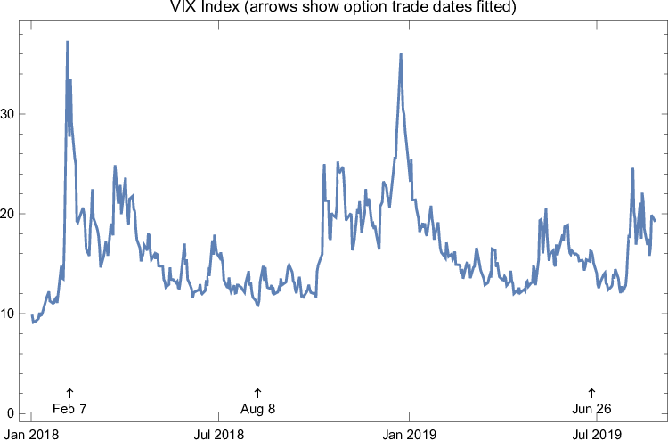
2 days after the “Volpocalypse” (VIX=27.73).
(Bands computed with CRRA ).

(Bands computed with CRRA ).

(Bands computed with CRRA ).

Trade date: Feb 7, 2018. Expiration date: Feb 12, 2018

Trade date: Feb 7, 2018. Expiration date: Feb 20, 2018

Trade date: Feb 7, 2018. Expiration date: Feb 12, 2018

PM minus AM option prices. Trade date: Feb 7, 2018. Expiration date: Mar 16, 2018
Top: Market Data (dots) + original GMM fit to market mid-quotes (curve).
Middle: Original GMM fit.
Bottom: GMM fit to adjusted market quotes: Solid=PM adjusted. Dashed=AM adjusted.

PM minus AM option prices. Trade date: Feb 7, 2018. Expiration date: Dec 21, 2018
Top: Market Data (dots) + original GMM fit to market mid-quotes (curve).
Middle: Original GMM fit.
Bottom: GMM fit to adjusted market quotes: Solid=PM adjusted. Dashed=AM adjusted.


10 Appendix A – representative agent/power utility model
10.1 General theory
Consider a discrete-time securities market with a probability measure ℙ, information flow , and time- conditional expectations . The fundamental theorem of asset pricing provides that, under the absence of arbitrage opportunities, there exists a positive stochastic discount factor (process) that prices every traded security via:2020 20 A careful textbook treatment is found in Back (2010).
| (24) |
Note that is a random variable at time , whose value is fully revealed by time ; thus . Critically, the same stochastic discount factor process prices every security. Recalling our earlier notation, for risk-free discount bonds maturing at , , and so
| (25) |
Thus (24) is equivalent to a discounted expectation under an inferred ℚ-measure, via
| (26) |
Next, our representative agent model fleshes this out – makes explicit – and we’ll show leads to the previous relation (6) for the change of measures.
10.2 A representative agent with power utility
We assume security prices are set by a representative agent with time- (‘today’) wealth , investment horizon , who makes portfolio choices to maximize an expected power utility function of return:
| (27) |
Here is a time-impatience rate and is the Arrow-Pratt CRRA. When , the agent is strictly risk-averse, and when , risk-neutral. When the term inside the bracket is interpreted as . At time-, the agent’s investment universe contains three traded securities:
- •
A risk-free bond, here a contract between individuals, with deterministic (non-random) price .
- •
A broad-based positive (equity) market index , with future random price . This is a total-return index, which includes reinvested dividends.
- •
A generic contingent claim, also a contract between individuals, with today’s price , maturity , and buyer payoff with generic payoff function .
Implicitly, the equity index is the sole source of uncertainty. Since the risk-free bond, as described, is a type of ‘generic contingent claim’, it’s redundant in the above list. But there is no harm singling it out. The agent optimally allocates wealth fractions: to the discount bond, to the generic contingent claim, and to stocks. The agent’s optimization problem is:
| (28) |
Next, we assume a stable, market-clearing equilibrium exists. By that, we mean the following two conditions hold. First, is a twice-differentiable, concave function of for all , strictly increasing for . Second, the agent’s optimal solution for lies at . In other words, the equity index must absorb 100% of the representative agent’s wealth , and any other allocation is inferior. The other securities (the discount bond and the derivative) do exist and are traded in this market. But as contracts between individuals (like puts, calls, and futures), they are in zero net supply.
The first condition implies ; i.e., the equity risk premium, , must be positive. Concavity implies , where
| (29) |
By assumption, the expectation in (29) exists, and it’s seen to be manifestly positive; our stability conditions then require that : the agent is strictly risk-averse.
The second condition implies the two first order conditions hold:
which yields:
| (30) |
Substituting the denominator for with the same denominator from yields
| (31) |
Since the contingent claim payoff is an arbitrary function of , (31) is a version of (26). Indeed, we must have , for some non-random . Since , comparing with the first equation in (30) says . Summarizing, under our market-clearing equilibrium model with power utility,
| (32) |
One can also check that, as required by (24), we have .
Recall our previous notations: . Also, recall and denote the corresponding total-return pdf’s, and . Using those notations, the second equation in (31) may be written:
| (33) |
Now specialize to the particular payoff , where is an arbitrary real number, and is the Dirac delta. In other words, . With that payoff, (33) reads
| (34) |
In the reverse direction, (34) implies , where is a constant independent of . Since is a probability density, is determined and so
| (35) |
Equations (34)-(35) are the density transformations used in the main body at (6) or given formally at (22). They were asserted to follow from our representative agent model, and now we’ve shown that they do.
| File/ | Expiration | Put- | Bid-Ask | Convergence | ERP | Run | |||
|---|---|---|---|---|---|---|---|---|---|
| Root | Date (days-to-go) | BidMin | N | PG | OutStats | (steps) | time | ||
| 1 SPXW | Feb 9, 2018 (2) | 0.05 | 5 | 5 | 139 | A(1,0.05) | No(250) | 26.34 | 1055 |
| 2 SPXW | Feb 12, 2018 (5) | 0.05 | 5 | 5 | 127 | G(0,0) | Yes(133) | 16.21 | 484 |
| 3 SPXW | Feb 14, 2018 (7) | 0.05 | 5 | 5 | 142 | A(1,0.01) | Yes(115) | 16.16 | 538 |
| 4 SPX | Feb 16, 2018 (9) | 0.05 | 5 | 5 | 239 | A(1,0.08) | Yes(174) | 15.73 | 1076 |
| 5 SPXW | Feb 16, 2018 (9) | 0.05 | 5 | 5 | 228 | A(1,0.03) | No(250) | 15.93 | 1554 |
| 6 SPXW | Feb 20, 2018 (13) | 0.05 | 5 | 5 | 147 | A(2,0.03) | Yes(75) | 12.26 | 312 |
| 7 SPXW | Feb 21, 2018 (14) | 0.05 | 5 | 5 | 148 | G(0,0) | Yes(66) | 12.43 | 263 |
| 8 SPXW | Feb 23, 2018 (16) | 0.05 | 5 | 5 | 185 | G(0,0) | Yes(118) | 12.78 | 719 |
| 9 SPXW | Feb 26, 2018 (19) | 0.05 | 4 | 5 | 145 | G(0,0) | Yes(198) | 11.34 | 412 |
| 10 SPXW | Feb 28, 2018 (21) | 0.40 | 4 | 5 | 175 | A(1,0.06) | Yes(102) | 11.80 | 426 |
| 11 SPXW | Mar 2, 2018 (23) | 0.05 | 4 | 5 | 199 | G(0,0) | No(250) | 12.14 | 985 |
| 12 SPXW | Mar 5, 2018 (26) | 0.05 | 4 | 5 | 128 | A(1,0.11 | Yes(65) | 10.93 | 156 |
| 13 SPXW | Mar 7, 2018 (28) | 0.05 | 4 | 5 | 131 | G(0,0) | Yes(44) | 10.91 | 135 |
| 14 SPXW | Mar 9, 2018 (30) | 0.05 | 4 | 5 | 176 | A(1,0.02) | Yes(79) | 11.54 | 305 |
| 15 SPXW | Mar 12, 2018 (33) | 0.05 | 4 | 5 | 127 | G(0,0) | Yes(35) | 10.21 | 86 |
| 16 SPXW | Mar 14, 2018 (35) | 0.05 | 4 | 5 | 104 | G(0,0) | Yes(103) | 10.20 | 135 |
| 17 SPX | Mar 16, 2018 (37) | 0.05 | 4 | 5 | 259 | G(0,0) | Yes(77) | 10.43 | 309 |
| 18 SPXW | Mar 16, 2018 (37) | 0.05 | 4 | 5 | 259 | A(1,0.01) | Yes(217) | 10.39 | 878 |
| 19 SPXW | Mar 23, 2018 (44) | 0.05 | 4 | 5 | 159 | G(0,0) | Yes(42) | 10.01 | 167 |
| 20 SPXW | Mar 29, 2018 (50) | 0.05 | 4 | 5 | 198 | G(0,0) | Yes(59) | 9.55 | 236 |
| 21 SPXW | Apr 6, 2018 (58) | 0.05 | 4 | 5 | 143 | G(0,0) | Yes(90) | 8.93 | 333 |
| 22 SPX | Apr 20, 2018 (72) | 0.05 | 4 | 5 | 244 | A(1,0.08) | Yes(64) | 8.72 | 269 |
| 23 SPXW | Apr 20, 2018 (72) | 0.05 | 5 | 5 | 246 | A(2,0.01) | Yes(156) | 8.64 | 1046 |
| 24 SPXW | Apr 30, 2018 (82) | 0.05 | 4 | 5 | 106 | G(0,0) | Yes(137) | 8.39 | 177 |
| 25 SPX | May 18, 2018 (100) | 0.05 | 4 | 5 | 168 | G(0,0) | Yes(35) | 8.52 | 126 |
| 26 SPXW | May 18, 2018 (100) | 0.05 | 4 | 5 | 167 | G(0,0) | Yes(44) | 8.50 | 163 |
| 27 SPXW | May 31, 2018 (113) | 0.05 | 4 | 5 | 60 | G(0,0) | Yes(73) | 8.25 | 86 |
| 28 SPX | Jun 15, 2018 (128) | 0.05 | 4 | 5 | 93 | A(1,0.04) | No(250) | 8.23 | 306 |
| 29 SPXW | Jun 15, 2018 (128) | 0.05 | 4 | 5 | 95 | A(2,0.05) | Yes(95) | 8.17 | 115 |
| 30 SPXW | Jun 29, 2018 (142) | 0.05 | 4 | 5 | 167 | G(0,0) | Yes(29) | 8.10 | 107 |
| 31 SPXW | Jul 31, 2018 (174) | 0.05 | 4 | 5 | 87 | G(0,0) | Yes(34) | 7.79 | 43 |
| 32 SPX | Sep 21, 2018 (226) | 0.05 | 4 | 5 | 86 | G(0,0) | Yes(109) | 7.56 | 132 |
| 33 SPXW | Sep 21, 2018 (226) | 0.05 | 4 | 5 | 87 | G(0,0) | Yes(46) | 7.53 | 55 |
| 34 SPXW | Sep 28, 2018 (233) | 0.05 | 4 | 5 | 63 | G(0,0) | Yes(90) | 7.52 | 109 |
| 35 SPX | Dec 21, 2018 (317) | 0.05 | 4 | 5 | 105 | A(1,0.05) | No(250) | 7.37 | 324 |
| 36 SPXW | Dec 21, 2108 (317) | 0.05 | 4 | 5 | 98 | G(0,0) | Yes(63) | 7.36 | 76 |
| 37 SPXW | Dec 31, 2018 (327) | 0.05 | 4 | 5 | 62 | G(0,0) | Yes(44) | 7.47 | 53 |
| 38 SPX | Jan 18, 2019 (345) | 0.05 | 4 | 5 | 89 | G(0,0) | Yes(39) | 7.25 | 47 |
| 39 SPX | Mar 15, 2019 (401) | 0.05 | 4 | 5 | 85 | G(0,0) | Yes(147) | 7.29 | 176 |
| 40 SPX | Jun 21, 2019 (499) | 0.05 | 4 | 5 | 92 | G(0,0) | Yes(60) | 7.28 | 73 |
| 41 SPX | Dec 20, 2019 (681) | 0.30 | 4 | 5 | 93 | G(0,0) | No(250) | 7.23 | 309 |
| 42 SPX | Dec 18, 2020 (1045) | 0.30 | 4 | 5 | 96 | G(0,0) | No(250) | 7.67 | 301 |
| File/ | Expiration | Put- | Bid-Ask | Convergence | ERP | Run | |||
|---|---|---|---|---|---|---|---|---|---|
| Root | Date (days-to-go) | BidMin | N | PG | OutStats | (steps) | time | ||
| 1 SPXW | Aug 10, 2018 (2) | 0.10 | 5 | 5 | 31 | G(0,0) | Yes(63) | 2.02 | 120 |
| 2 SPXW | Aug 13, 2018 (5) | 0.10 | 5 | 5 | 51 | G(0,0) | Yes(62) | 1.45 | 119 |
| 3 SPXW | Aug 15, 2018 (7) | 0.10 | 5 | 5 | 87 | A(2,0.01) | Yes(76) | 1.87 | 183 |
| 4 SPX | Aug 17, 2018 (9) | 0.10 | 5 | 5 | 112 | A(2,0.01) | Yes(67) | 2.06 | 361 |
| 5 SPXW | Aug 17, 2018 (9) | 0.10 | 5 | 5 | 119 | A(2,0.02) | Yes(73) | 2.18 | 463 |
| 6 SPXW | Aug 20, 2018 (12) | 0.10 | 5 | 5 | 117 | G(0,0) | Yes(57) | 1.99 | 356 |
| 7 SPXW | Aug 22, 2018 (14) | 0.10 | 5 | 5 | 122 | G(0,0) | Yes(68) | 2.22 | 439 |
| 8 SPXW | Aug 24, 2018 (16) | 0.10 | 5 | 5 | 162 | G(0,0) | No(250) | 2.43 | 1623 |
| 9 SPXW | Aug 27, 2018 (19) | 0.10 | 5 | 5 | 121 | G(1,0.00) | No(250) | 2.30 | 1506 |
| 10 SPXW | Aug 29, 2018 (21) | 0.10 | 5 | 5 | 106 | A(1,0.01) | No(250) | 2.48 | 1316 |
| 11 SPXW | Aug 31, 2018 (23) | 0.10 | 5 | 5 | 164 | G(1,0.00) | No(250) | 2.67 | 1589 |
| 12 SPXW | Sep 4, 2018 (27) | 0.10 | 5 | 5 | 109 | A(2,0.04) | No(250) | 2.49 | 1321 |
| 13 SPXW | Sep 5, 2018 (28) | 0.10 | 5 | 5 | 109 | A(2,0.04) | No(250) | 2.53 | 1288 |
| 14 SPXW | Sep 7, 2018 (30) | 0.20 | 5 | 5 | 164 | A(1,0.02) | No(250) | 2.70 | 1714 |
| 15 SPXW | Sep 10, 2018 (33) | 0.10 | 5 | 5 | 111 | A(2,0.02) | No(250) | 2.62 | 1307 |
| 16 SPXW | Sep 12, 2018 (35) | 0.10 | 5 | 5 | 105 | G(0,0) | No(250) | 2.75 | 1279 |
| 17 SPXW | Sep 14, 2018 (37) | 0.10 | 5 | 5 | 166 | A(2,0.03) | No(250) | 2.87 | 1612 |
| 18 SPX | Sep 21, 2018 (44) | 0.20 | 5 | 5 | 236 | A(1,0.01) | No(250) | 3.07 | 1631 |
| 19 SPXW | Sep 21, 2018 (44) | 0.20 | 5 | 5 | 236 | A(1,0.01 | No(250) | 3.11 | 1601 |
| 20 SPXW | Sep 28, 2018 (51) | 0.10 | 5 | 5 | 205 | A(1,0.03) | No(250) | 3.33 | 1594 |
| 21 SPXW | Oct 5, 2018 (58) | 0.10 | 5 | 5 | 151 | G(0,0) | Yes(187) | 3.43 | 1210 |
| 22 SPXW | Oct 12, 2018 (65) | 0.10 | 5 | 5 | 151 | G(0,0) | Yes(224) | 3.52 | 1405 |
| 23 SPX | Oct 19, 2018 (72) | 0.10 | 5 | 5 | 248 | A(1,0.03) | No(250) | 3.60 | 1598 |
| 24 SPXW | Oct 19, 2018 (72) | 0.10 | 5 | 5 | 247 | G(0,0) | No(250) | 3.63 | 1591 |
| 25 SPXW | Oct 31, 2018 (84) | 0.10 | 5 | 5 | 167 | A(2,0.01) | Yes(121) | 3.80 | 756 |
| 26 SPX | Nov 16, 2018 (100) | 0.10 | 5 | 5 | 238 | A(1,0.05) | No(250) | 4.11 | 1572 |
| 27 SPXW | Nov 16, 2018 (100) | 0.10 | 5 | 5 | 238 | A(1,0.01) | No(250) | 4.15 | 1589 |
| 28 SPXW | Nov 30, 2108 (114) | 0.10 | 5 | 5 | 100 | G(1,0.00) | Yes(108) | 4.29 | 533 |
| 29 SPX | Dec 21, 2018 (135) | 0.10 | 5 | 5 | 95 | A(2,0.06) | Yes(223) | 4.44 | 571 |
| 30 SPXW | Dec 21, 2018 (135) | 0.20 | 5 | 5 | 96 | G(0,0) | No(250) | 4.45 | 676 |
| 31 SPXW | Dec 31, 2018 (145) | 0.10 | 5 | 5 | 189 | G(0,0) | Yes(90) | 4.42 | 564 |
| 32 SPX | Jan 18, 2019 (163) | 0.10 | 5 | 5 | 91 | G(1,0.00) | No(250) | 4.54 | 663 |
| 33 SPXW | Jan 31, 2019 (176) | 0.10 | 5 | 5 | 92 | G(0,0) | Yes(72) | 4.70 | 180 |
| 34 SPX | Mar 15, 2019 (219) | 0.10 | 5 | 5 | 89 | G(0,0) | Yes(147) | 4.81 | 445 |
| 35 SPXW | Mar 29, 2109 (233) | 0.10 | 5 | 5 | 87 | G(0,0) | Yes(95) | 4.90 | 234 |
| 36 SPX | Jun 21, 2019 (317) | 0.10 | 5 | 5 | 94 | G(0,0) | Yes(44) | 5.20 | 126 |
| 37 SPXW | Jun 21, 2019 (317) | 0.10 | 5 | 5 | 94 | G(0,0) | Yes(32) | 5.21 | 80 |
| 38 SPXW | Jun 28, 2019 (324) | 0.10 | 5 | 5 | 86 | G(0,0) | Yes(122) | 5.28 | 301 |
| 39 SPX | Sep 20, 2019 (408) | 0.10 | 5 | 5 | 89 | G(0,0) | Yes(46) | 5.50 | 125 |
| 40 SPX | Dec 20, 2019 (499) | 0.10 | 5 | 5 | 104 | G(0,0) | Yes(80) | 6.02 | 493 |
| 41 SPX | Jun 19, 2019 (681) | 0.10 | 5 | 5 | 89 | G(0,0) | Yes(113) | 5.92 | 353 |
| 42 SPX | Dec 18, 2020 (863) | 0.20 | 5 | 5 | 100 | G(0,0) | Yes(153) | 7.09 | 911 |
After(+): Market prices for PM options (asterisks) are adjusted upward.
After(-): Market prices for AM options (asterisks) are adjusted downward.
| I. Before | |||||||||
| File/ | Expiration | Put- | Bid-Ask | Convergence | ERP | Run | |||
| Root | Date (days-to-go) | BidMin | N | PG | OutStats | (steps) | time | ||
| 17 SPX | Mar 16, 2018 (37) | 0.05 | 4 | 5 | 259 | G(0,0) | Yes(77) | 10.43 | 309 |
| 18 SPXW | Mar 16, 2018 (37) | 0.05 | 4 | 5 | 259 | A(1,0.01) | Yes(217) | 10.39 | 878 |
| 35 SPX | Dec 21, 2018 (317) | 0.05 | 4 | 5 | 105 | A(1,0.05) | No(250) | 7.37 | 324 |
| 36 SPXW | Dec 21, 2108 (317) | 0.05 | 4 | 5 | 98 | G(0,0) | Yes(63) | 7.36 | 76 |
| II. After(+) | |||||||||
| File/ | Expiration | Put- | Bid-Ask | Convergence | ERP | Run | |||
| Root | Date (days-to-go) | BidMin | N | PG | OutStats | (steps) | time | ||
| 17 SPX | Mar 16, 2018 (37) | 0.05 | 4 | 5 | 259 | G(0,0) | Yes(59) | 10.42 | 251 |
| 18 SPXW∗ | Mar 16, 2018 (37) | 0.05 | 4 | 5 | 259 | A(1,0.01) | Yes(52) | 10.58 | 216 |
| 35 SPX | Dec 21, 2018 (317) | 0.15 | 4 | 5 | 97 | G(0,0) | Yes(71) | 7.35 | 88 |
| 36 SPXW∗ | Dec 21, 2108 (317) | 0.15 | 4 | 5 | 97 | G(0,0) | Yes(85) | 7.39 | 105 |
| III. After(-) | |||||||||
| File/ | Expiration | Put- | Bid-Ask | Convergence | ERP | Run | |||
| Root | Date (days-to-go) | BidMin | N | PG | OutStats | (steps) | time | ||
| 17 SPX∗ | Mar 16, 2018 (37) | 0.05 | 4 | 5 | 259 | G(0,0) | Yes(90) | 10.20 | 350 |
| 18 SPXW | Mar 16, 2018 (37) | 0.05 | 4 | 5 | 259 | A(1,0.01) | Yes(217) | 10.40 | 854 |
| 35 SPX∗ | Dec 21, 2018 (317) | 0.15 | 4 | 5 | 97 | G(0,0) | Yes(73) | 7.32 | 75 |
| 36 SPXW | Dec 21, 2108 (317) | 0.15 | 4 | 5 | 97 | G(0,0) | Yes(85) | 7.36 | 88 |
Rates shown as %/year. Forward = , where .
| File/ | VIX white paper method | PC-parity regression method | Realized | |||||||
|---|---|---|---|---|---|---|---|---|---|---|
| Root | (Years) | Forward | ERP | Forward | ERP | |||||
| 1 SPXW | 0.00551 | 1.24 | 10.77 | 2705.06 | 26.34 | 5.69 | 14.75 | 2705.13 | 26.35 | 8.36 |
| 2 SPXW | 0.01373 | 1.25 | 6.02 | 2704.71 | 16.21 | 2.91 | 7.03 | 2704.95 | 16.23 | 3.59 |
| 3 SPXW | 0.01921 | 1.26 | 5.82 | 2704.11 | 16.16 | 5.44 | 9.55 | 2704.35 | 16.25 | 4.29 |
| 4 SPX | 0.02394 | 1.27 | 5.16 | 2703.96 | 15.73 | 3.33 | 7.55 | 2703.73 | 15.75 | 4.69 |
| 5 SPXW | 0.02469 | 1.27 | 5.64 | 2703.56 | 15.93 | 1.70 | 5.80 | 2703.74 | 15.92 | 4.69 |
| 6 SPXW | 0.03565 | 1.28 | 3.59 | 2704.26 | 12.26 | 2.88 | 4.91 | 2704.53 | 12.30 | 3.45 |
| 7 SPXW | 0.03838 | 1.29 | 3.19 | 2704.51 | 12.43 | 3.05 | 4.76 | 2704.70 | 12.43 | 3.25 |
| 8 SPXW | 0.04386 | 1.30 | 2.75 | 2704.76 | 12.78 | 2.74 | 4.13 | 2704.84 | 12.79 | 3.18 |
| 9 SPXW | 0.05208 | 1.31 | 2.78 | 2704.41 | 11.34 | 2.72 | 4.01 | 2704.67 | 11.41 | 2.92 |
| 10 SPXW | 0.05756 | 1.32 | 2.71 | 2704.31 | 11.80 | 2.09 | 3.36 | 2704.50 | 11.82 | 3.07 |
| 11 SPXW | 0.06304 | 1.32 | 2.86 | 2703.86 | 12.14 | 2.48 | 3.92 | 2704.02 | 12.16 | 3.20 |
| 12 SPXW | 0.07126 | 1.34 | 2.51 | 2704.21 | 10.93 | 2.75 | 3.67 | 2704.72 | 10.94 | 2.84 |
| 13 SPXW | 0.07674 | 1.34 | 2.36 | 2704.36 | 10.91 | 2.39 | 3.37 | 2704.44 | 10.94 | 2.80 |
| 14 SPXW | 0.08222 | 1.35 | 2.35 | 2704.26 | 11.54 | 2.33 | 3.28 | 2704.37 | 11.56 | 2.97 |
| 15 SPXW | 0.09044 | 1.36 | 2.21 | 2704.41 | 10.21 | 2.18 | 2.98 | 2704.52 | 10.24 | 2.71 |
| 16 SPXW | 0.09592 | 1.37 | 2.36 | 2703.91 | 10.20 | 2.22 | 3.14 | 2704.11 | 10.21 | 2.91 |
| 17 SPX | 0.10066 | 1.38 | 2.38 | 2703.76 | 10.43 | 2.41 | 3.27 | 2704.14 | 10.45 | 2.85 |
| 18 SPXW | 0.10140 | 1.38 | 2.31 | 2703.91 | 10.39 | 2.35 | 3.25 | 2704.03 | 10.42 | 2.85 |
| 19 SPXW | 0.12058 | 1.40 | 1.77 | 2705.26 | 10.01 | 2.33 | 2.64 | 2705.48 | 10.03 | 2.54 |
| 20 SPXW | 0.13702 | 1.42 | 1.78 | 2705.16 | 9.55 | 2.31 | 2.61 | 2705.38 | 9.57 | 2.39 |
| 21 SPXW | 0.15893 | 1.45 | 1.54 | 2706.06 | 8.93 | 2.30 | 2.36 | 2706.22 | 8.96 | 2.24 |
| 22 SPX | 0.19655 | 1.49 | 1.46 | 2706.61 | 8.72 | 2.37 | 2.31 | 2706.80 | 8.75 | 2.15 |
| 23 SPXW | 0.19729 | 1.49 | 1.46 | 2706.61 | 8.64 | 2.39 | 2.34 | 2706.74 | 8.67 | 2.15 |
| 24 SPXW | 0.22469 | 1.52 | 1.33 | 2707.60 | 8.39 | 2.40 | 2.20 | 2707.70 | 8.42 | 1.94 |
| 25 SPX | 0.27326 | 1.56 | 1.52 | 2706.80 | 8.52 | 2.43 | 2.38 | 2706.85 | 8.56 | 2.23 |
| 26 SPXW | 0.27400 | 1.56 | 1.51 | 2706.90 | 8.50 | 2.46 | 2.41 | 2706.83 | 8.56 | 2.23 |
| 27 SPXW | 0.30962 | 1.69 | 1.55 | 2706.84 | 8.25 | 2.30 | 2.21 | 2707.24 | 8.31 | 2.19 |
| 28 SPX | 0.34997 | 1.62 | 1.55 | 2707.15 | 8.23 | 2.42 | 2.35 | 2707.20 | 8.28 | 2.20 |
| 29 SPXW | 0.35071 | 1.62 | 1.55 | 2707.20 | 8.17 | 2.28 | 2.23 | 2706.91 | 8.21 | 2.20 |
| 30 SPXW | 0.38907 | 1.65 | 1.45 | 2708.60 | 8.10 | 2.36 | 2.15 | 2708.69 | 8.15 | 2.08 |
| 31 SPXW | 0.47674 | 1.70 | 1.34 | 2711.22 | 7.79 | 2.36 | 1.97 | 2711.54 | 7.87 | 1.94 |
| 32 SPX | 0.61847 | 1.77 | 1.37 | 2713.13 | 7.56 | 2.44 | 2.06 | 2712.93 | 7.62 | 2.06 |
| 33 SPXW | 0.61921 | 1.77 | 1.39 | 2712.88 | 7.53 | 2.37 | 1.98 | 2713.05 | 7.58 | 2.06 |
| 34 SPXW | 0.63839 | 1.78 | 1.39 | 2713.13 | 7.52 | 2.36 | 1.97 | 2713.22 | 7.58 | 2.05 |
| 35 SPX | 0.86778 | 1.86 | 1.36 | 2718.10 | 7.37 | 2.43 | 1.94 | 2718.11 | 7.46 | 2.05 |
| 36 SPXW | 0.86852 | 1.86 | 1.34 | 2718.76 | 7.36 | 2.41 | 1.90 | 2718.68 | 7.43 | 2.05 |
| 37 SPXW | 0.89592 | 1.86 | 1.26 | 2721.30 | 7.47 | 2.49 | 1.88 | 2721.31 | 7.54 | 2.04 |
| 38 SPX | 0.94449 | 1.88 | 1.27 | 2722.01 | 7.25 | 2.51 | 1.90 | 2722.19 | 7.33 | 2.02 |
| 39 SPX | 1.09792 | 1.92 | 1.33 | 2723.99 | 7.29 | 2.44 | 1.85 | 2724.18 | 7.37 | 2.07 |
| 40 SPX | 1.36641 | 1.98 | 1.36 | 2729.63 | 7.28 | 2.44 | 1.80 | 2730.22 | 7.39 | 2.07 |
| 41 SPX | 1.86504 | 2.10 | 1.40 | 2741.85 | 7.23 | 2.44 | 1.73 | 2742.68 | 7.29 | NA |
| 42 SPX | 2.86230 | 2.29 | 1.44 | 2772.82 | 7.67 | 2.54 | 1.69 | 2772.77 | 7.78 | NA |
Rates shown as %/year. Forward = , where .
| File/ | VIX white paper method | PC-parity regression method | |||||||
|---|---|---|---|---|---|---|---|---|---|
| Root | (Years) | Forward | ERP | Forward | ERP | ||||
| 1 SPXW | 0.00551 | 1.85 | 7.63 | 2860.68 | 2.02 | 5.75 | 11.90 | 2860.62 | 2.01 |
| 2 SPXW | 0.01373 | 1.86 | 3.67 | 2860.88 | 1.45 | 1.95 | 3.95 | 2860.80 | 1.45 |
| 3 SPXW | 0.01921 | 1.86 | 4.06 | 2860.38 | 1.87 | 2.13 | 4.41 | 2860.34 | 1.87 |
| 4 SPX | 0.02394 | 1.87 | 4.22 | 2859.98 | 2.06 | 2.66 | 4.98 | 2860.00 | 2.06 |
| 39 SPX | 1.11709 | 2.44 | 1.57 | 2889.55 | 5.50 | 2.85 | 1.97 | 2889.55 | 5.54 |
| 40 SPX | 1.36641 | 2.50 | 1.57 | 2898.22 | 6.02 | 2.88 | 1.80 | 2898.19 | 5.83 |
| 41 SPX | 1.86504 | 2.62 | 1.60 | 2916.26 | 5.92 | 3.01 | 1.99 | 2916.37 | 6.09 |
| 42 SPX | 2.36367 | 2.71 | 1.66 | 2933.67 | 7.09 | 3.05 | 2.00 | 2934.01 | 7.00 |
References
- Back ((2010)) Back, K.E. (2010). Asset Pricing and Portfolio Choice Theory. : Oxford Univ. Press.
- Bliss & Panigirtzoglou ((2004)) Bliss, R.R. & Panigirtzoglou, N. (2004). Option-implied risk aversion estimates. The Journal of Finance 59 1 407-446.
- Carr & Yu ((2012)) Carr, P. & Yu, J. (2012). Risk, Return, and Ross Recovery. The Journal of Derivatives 20 1 38-59.
- Duarte & Rosa ((2015)) Duarte, F. & Rosa, C. (2015). The Equity Risk Premium: A Review of Models [Staff report, Federal Reserve Bank of New York].
- Fengler ((2005)) Fengler, M.R. (2005). Arbitrage-Free Smoothing of the Implied Volatility Surface Tech. Rep.. : Humboldt University of Berlin. SFB 649 Discussion paper 2005-019
- Figlewski ((2010)) Figlewski, S. (2010). Estimating the Implied Risk Neutral Density for the U.S. Market Portfolio. In T. Bollerslev, J. Russell & M. Watson (Eds.), Volatility and Time Series Econometrics: Essays in Honor of Robert F. Engle. : Oxford Univ. Press.
- Friend & Blume ((1975)) Friend, I. & Blume, M.E. (1975). The Demand for Risky Assets. Amer. Econ. Review 900-922.
- Gatheral & Jacquier ((2013)) Gatheral, J. & Jacquier, A. (2013). Arbitrage-free SVI volatility surfaces. arXiv:q-fin.PR/1204.0646v4
- Hammond et al. ((2011)) Hammond, P., Leibowitz, M. & Siegel, L. (Eds.). (2011). Rethinking the Equity Risk Premium. : CFA Institute.
- Ibbotson & Duff & Phelps ((2016)) Ibbotson, R.G. & Duff & Phelps. (2016). 2016 SBBI yearbook. : Wiley.
- Lewis ((2020)) Lewis, A.L. (2020). US Equity Risk Premiums during the COVID-19 Pandemic. arXiv:2004.13871 [q-fin.GN].
- Malz ((2014)) Malz, A.M. (2014). A Simple and Reliable Way to Compute Option-Based Risk-Neutral Distributions [Staff report, Federal Reserve Bank of New York].
- Qin & Linetsky ((2016)) Qin, L. & Linetsky, V. (2016). Positive eigenfunctions of Markovian pricing operators: Hansen-Scheinkman factorization, Ross recovery and Long-term pricing. Operations Research 64 1 99-117.
- Ross ((2015)) Ross, S. (2015). The recovery theorem. The Journal of Finance 70 615-648.
- Walden ((2016)) Walden, J. (2016). Recovery with unbounded diffusion processes. Review of Finance 21 4 1-42.