Randomized linear algebra for model reduction.
Part II: minimal residual methods and dictionary-based approximation.
Abstract
A methodology for using random sketching in the context of model order reduction for high-dimensional parameter-dependent systems of equations was introduced in [Balabanov and Nouy 2019, Part I]. Following this framework, we here construct a reduced model from a small, efficiently computable random object called a sketch of a reduced model, using minimal residual methods. We introduce a sketched version of the minimal residual based projection as well as a novel nonlinear approximation method, where for each parameter value, the solution is approximated by minimal residual projection onto a subspace spanned by several vectors picked (online) from a dictionary of candidate basis vectors. It is shown that random sketching technique can improve not only efficiency but also numerical stability. A rigorous analysis of the conditions on the random sketch required to obtain a given accuracy is presented. These conditions may be ensured a priori with high probability by considering for the sketching matrix an oblivious embedding of sufficiently large size. Furthermore, a simple and reliable procedure for a posteriori verification of the quality of the sketch is provided. This approach can be used for certification of the approximation as well as for adaptive selection of the size of the random sketching matrix.
Keywords— model order reduction, reduced basis, random sketching, subspace embedding, minimal residual methods, sparse approximation, dictionary
1 Introduction
We consider large parameter-dependent systems of equations
| (1) |
where is a solution vector, is a parameter-dependent matrix, is a parameter-dependent right hand side and is a parameter set. Parameter-dependent problems are considered for many purposes such as design, control, optimization, uncertainty quantification or inverse problems.
Solving (1) for many parameter values can be computationally unfeasible. Moreover, for real-time applications, a quantity of interest ( or a function of ) has to be estimated on the fly in highly limited computational time for a certain value of . Model order reduction (MOR) methods are developed for efficient approximation of the quantity of interest for each parameter value. They typically consist of two stages. In the first so-called offline stage a reduced model is constructed from the full order model. This stage usually involves expensive computations such as evaluations of for several parameter values, computing multiple high-dimensional matrix-vector and inner products, etc., but this stage is performed only once. Then, for each given parameter value, the precomputed reduced model is used for efficient approximation of the solution or an output quantity with a computational cost independent of the dimension of the initial system of equations (1). For a detailed presentation of the classical MOR methods such as Reduced Basis (RB) method and Proper Orthogonal Decomposition (POD) the reader can refer to [5]. In the present work the approximation of the solution shall be obtained with a minimal residual (minres) projection on a reduced (possibly parameter-dependent) subspace. The minres projection can be interpreted as a Petrov-Galerkin projection where the test space is chosen to minimize some norm of the residual [10, 1]. Major benefits over the classical Galerkin projection include an improved stability (quasi-optimality) for non-coercive problems and more effective residual-based error bounds of an approximation (see e.g. [10]). In addition, minres methods are better suited to random sketching as will be seen in the present article.
In recent years randomized linear algebra (RLA) became a popular approach in the fields such as data analysis, machine learning, compressed sensing, etc. [43, 35, 42]. This probabilistic approach for numerical linear algebra can yield a drastic computational cost reduction in terms of classical metrics of efficiency such as complexity (number of flops) and memory consumption. Moreover, it can be highly beneficial in extreme computational environments that are typical in contemporary scientific computing. For instance, RLA can be essential when data has to be analyzed only in one pass (e.g., when it is streamed from a server) or when it is distributed on multiple workstations with expensive communication costs.
Despite their indisputable success in fields closely related to MOR, the aforementioned techniques only recently started to be extensively used in MOR community. One of the earliest works considering RLA in the context of MOR is [44], where the authors proposed to use RLA for interpolation of (implicit) inverse of a parameter-dependent matrix. In [9] the RLA was used for approximating the range of a transfer operator and for computing a probabilistic bound for the approximation error. In [11, 26, 39] the authors developed probabilistic error estimators based on random projections and the adjoint method. These approaches can also be formulated in RLA framework. A randomized singular value decomposition (see [24, 43]) was used for computing the POD vectors in [25]. Efficient algorithms for Dynamic Mode Decomposition based on RLA and compressed sensing were proposed in [21, 7, 22, 31, 8], though with a lack of theoretical analysis.
As already shown in [3], random sketching can lead to drastic reduction of the computational costs of classical MOR methods. A random sketch of a reduced model is defined as a set of small random projections of the reduced basis vectors and the associated residuals. Its representation (i.e, affine decomposition11 1 A parameter-dependent quantity with values in a vector space over is said to admit an affine representation if with and .) can be efficiently precomputed in basically any computational architecture. The random projections should be chosen according to the metric of efficiency, e.g., number of flops, memory consumption, communication cost between distributed machines, scalability, etc. A rigorous analysis of the cost of obtaining a random sketch in different computational environments can be found in [3, Section 4.4]. When a sketch has been computed, the reduced model can be approximated without operating on large vectors but only on their small sketches typically requiring negligible computational costs. The approximation can be guaranteed to almost preserve the quality of the original reduced model with user-specified probability. The computational cost depends only logarithmically on the probability of failure, which can therefore be chosen very small, say . In [3] it was shown how random sketching can be employed for an efficient approximation of the Galerkin projection, the computation of the norm of the residual for error estimation, and the computation of a primal-dual correction. Furthermore, new efficient sketched versions of the weak greedy algorithm and Proper Orthogonal Decomposition were introduced for generation of reduced bases.
The present work is a continuation of [3]. Here we adapt the random sketching technique to minimal residual methods, propose a novel dictionary-based approximation method and additionally discuss the questions of a posteriori certification of the sketch and efficient extraction of the output quantity from a solution of the reduced model.
1.1 Contributions and outline
First is proposed a method to approximate minres projection from a random sketch whose precomputation presents a much lower complexity, memory consumption and communication cost (see [3, Section 4.4] for details) than precomputation of affine decomposition of the reduced normal system of equations in the classical offline stage. The sketched minres projection is obtained online by solving a small least-squares problem, that can be more online-efficient and stable than solving the normal system of equations. Precise conditions on the sketch to yield (approximate) preservation of quasi-optimality constants of the standard minres projection are provided. The conditions do not depend on operator’s properties, which implies robustness for ill-conditioned and non-coercive problems in contrast to the sketched Galerkin methods [3].
In Section 4 we introduce a novel nonlinear method, where the solution to (1) is approximated by minres projection onto a subspace with basis picked online from a dictionary of candidate basis vectors. In Section 4.1 is shown why the dictionary-based approach is a more natural choice than the -refinement method [20, 19] or other partitioning methods, for problems where the solution is a superposition of several components (e.g., for PDEs with multiple transport phenomena). The dictionary-based approximation can be efficiently obtained online by solving a small sparse least-squares problem assembled from a random sketch of dictionary vectors, which entails practical feasibility of the method.
The potential of approximation with dictionaries for problems with a slow decay of the Kolmogorov -widths of the solution manifold was revealed in [18, 30]. Although they improved classical approaches, the algorithms proposed in [18, 30] still involve in general heavy computations in both offline and online stages, and can suffer from round-off errors. More specifically, the offline complexity and memory consumption associated with post-processing of the snapshots in [18, 30] are at least and , respectively, where is the cardinality of the dictionary and is the dimension of the original problem (1). With random sketching these costs may be reduced (by at least) a factor of . Furthermore, the online complexity and memory consumption of the approach in [30] are at least and , respectively, where is the dimension of the reduced approximation space. In its turn, our approach consumes (at least) and times less number of flops and amount of storage, respectively.
We also provide a probabilistic approach for a posteriori certification of the quality of (random) embedding and the associated sketch. The certification can be performed with a computational cost (much) less than the cost of obtaining the (sketched) reduced model’s solution. The proposed procedure can be particularly useful for adaptive selection of the size of a random sketching matrix since the a priori bounds can be pessimistic in practice [3].
Finally, in Appendix A we propose an approach, based on random sketching, for efficient extraction of linear/quadratic quantity of interest or primal-dual correction from the reduced model’s solution. It consists in first approximating the solution with a projection on a new (very small or sparse) reduced basis, that yields an efficiently computable approximation of the output quantity. Then this approximation is improved by a correction computable from sketches of the reduced bases with a negligible computational cost. This approach can be particularly important when considering a large approximation space or dictionary, with distributed/streamed basis vectors.
The outline of the article is as follows. In Section 2 we introduce the problem setting and recall the main ingredients of the framework developed in [3]. The minimal residual method considering a projection on a single low-dimensional subspace is discussed in Section 3. We present a standard minres projection in a discrete form followed by its efficient approximation with random sketching. Section 4 presents a novel dictionary-based minimal residual method using random sketching. A posteriori verification of the quality of a sketch and few scenarios where such a procedure can be used are provided in Section 5. The methodology is validated numerically on two nontrivial benchmark problems in Section 6. A discussion on the efficient and stable extraction of the quantity of interest from the reduced model’s solution is given in Appendix A.
2 Preliminaries
Let or and let and represent the solution space and its dual, respectively. The solution is an element from , is a linear operator from to , the right hand side and the extractor of the quantity of interest are elements of .
Spaces and are equipped with inner products and , where is the canonical -inner product on and is some symmetric (for ), or Hermitian (for ), positive definite operator. We denote by the canonical -norm on . Finally, for a matrix we denote by its (Hermitian) transpose.
2.1 Random sketching
A framework for using random sketching (see [24, 43]) in the context of MOR was introduced in [3]. The sketching technique is seen as a modification of the inner product in a given subspace (or a collection of subspaces). The modified inner product is an estimation of the original one and is much easier and more efficient to operate with. Next, we briefly recall the basic preliminaries from [3].
Let be a subspace of . The dual of is identified with a subspace of . For a matrix with we define the following semi-inner products on :
| (2) |
and we let and denote the associated semi-norms.
Definition 2.1.
A matrix is called a -subspace embedding (or simply an -embedding) for , if it satisfies
| (3) |
Here -embeddings shall be constructed as realizations of random matrices that are built in an oblivious way without any a priori knowledge of .
Definition 2.2.
A random matrix is called a oblivious subspace embedding if it is an -embedding for an arbitrary -dimensional subspace with probability at least .
Oblivious subspace embeddings (defined by Definition 2.1 with ) include the rescaled Gaussian distribution, the rescaled Rademacher distribution, the Subsampled Randomized Hadamard Transform (SRHT), the Subsampled Randomized Fourier Transform (SRFT), CountSketch matrix, SRFT combined with sequences of random Givens rotations, and others [3, 24, 43, 36]. In this work we shall rely on the rescaled Gaussian distribution and SRHT.
An oblivious subspace embedding for a general inner product can be constructed as
| (4) |
where is a subspace embedding and is an easily computable (possibly rectangular) matrix such that (see [3, Remark 2.7]).
It follows that an -subspace embedding for can be obtained with high probability as a realization of an oblivious subspace embedding of sufficiently large size. The number of rows for may be selected with the theoretical bounds from [3]. These bounds, however, can be pessimistic or even impractical (e.g., for adaptive algorithms or POD). In practice, one can consider of much smaller sizes and still obtain accurate subspace embeddings. When the conditions on the size of the sketch based on a priori analysis are too pessimistic, one can provide a posteriori guarantee. An easy and robust procedure for a posteriori verification of the quality of is provided in Section 5. The methodology can also be used for deriving a criterion for adaptive selection of the size of the random sketching matrix to satisfy the -embedding property with high probability.
2.2 A sketch of a reduced model
Here the output of a reduced order model is efficiently estimated from its random sketch. The -sketch of a reduced model associated with a subspace is defined as
| (5) |
where . Let be a matrix whose columns form a basis of . Then each element of (5) can be characterized from the coordinates of associated with , i.e., a vector such that , and the following quantities
| (6) |
Clearly and have affine expansions containing at most as many terms as the ones of and , respectively. The matrix and the affine expansions of and are referred to as the -sketch of (a representation of the -sketch of a reduced model associated with ). With a good choice of an oblivious embedding, a -sketch of can be efficiently precomputed in any computational environment (see [3]). Thereafter, an approximation of a reduced order model can be obtained with a negligible computational cost.
Note that in [3] the affine expansion of , where is an extractor of the linear quantity of interest , is also considered as a part of the -sketch of and is assumed to be efficiently computable. Let us address a scenario where the computation of the affine expansion of or its online evaluation is expensive. This may happen when has many terms in the affine expansion or when one considers a large approximation space (or dictionary) with possibly distributed basis vectors. In such a case, the output quantity can be approximated with an approach detailed in Appendix A. This method proceeds with two steps. First, the solution is approximated by a projection on a new basis , which is cheap to operate with (e.g, it has less columns than or the columns are sparse). The affine decomposition of an approximation of can now be efficiently precomputed. Then in the second step, the accuracy of is improved with a random sketching correction:
computable from the sketches , and with a negligible computational cost. Note that when interpreting random sketching as a Monte Carlo method, the proposed approach can be linked to a control variate variance reduction method where plays the role of the control variate for the estimation of . It is also important to note that the presented approach can be employed not only to extraction of a linear quantity of interest but also extraction of a quadratic quantity of interest or computation of the primal-dual correction.
3 Minimal residual projection
In this section we first present the standard minimal residual projection in a form that allows an easy introduction of random sketching. Then we introduce the sketched version of the minimal residual projection and provide conditions to guarantee its quality.
3.1 Standard minimal residual projection
Let be a subspace of (typically obtained with a greedy algorithm or approximate POD). The minres approximation of can be defined by
| (7) |
For linear problems it is equivalently characterized by the following (Petrov-)Galerkin orthogonality condition:
| (8) |
where .
If the operator is invertible then (7) is well-posed. In order to characterize the quality of the projection we define the following parameter-dependent constants
| (9a) | ||||
| (9b) | ||||
Let denote the orthogonal projection from on a subspace , defined for by
The constants and can be bounded by the minimal and maximal singular values of :
| (11a) | ||||
| (11b) | ||||
Bounds of and can be obtained theoretically [23] or numerically with the successive constraint method [27].
For each , the vector such that satisfies (8) can be obtained by solving the following reduced (normal) system of equations:
| (12) |
where and . The numerical stability of (12) can be ensured through orthogonalization of similarly as for the classical Galerkin projection. Such orthogonalization yields the following bound for the condition number of :
| (13) |
This bound can be insufficient for problems with matrix having a high or even moderate condition number.
The random sketching technique can be used to improve the efficiency and numerical stability of the minimal residual projection, as shown below.
3.2 Sketched minimal residual projection
Let be a certain subspace embedding. The sketched minres projection can be defined by (7) with the dual norm replaced by its estimation , which results in an approximation
| (14) |
The quasi-optimality of such a projection can be controlled in exactly the same manner as the quasi-optimality of the original minres projection. By defining the constants
| (15a) | ||||
| (15b) | ||||
we obtain the following result.
It follows that if and are almost equal to and , respectively, then the quasi-optimality of the original minres projection (7) shall be almost preserved by its sketched version (14). These properties of and can be guaranteed under some conditions on (see Proposition 3.3).
Proposition 3.3.
Define the subspace
| (17) |
If is a -subspace embedding for , then
| (18) |
Proof.
See Appendix B. ∎
An embedding satisfying an -subspace embedding property for the subspace defined in (17), for all simultaneously, with high probability, may be generated from an oblivious embedding of sufficiently large size. Note that . The number of rows of the oblivious embedding may be selected a priori using the bounds provided in [3], along with a union bound for the probability of success or the fact that is contained in a low-dimensional space. Alternatively, a better value for can be chosen with a posteriori procedure explained in Section 5. Note that if (18) is satisfied then the quasi-optimality constants of the minres projection are guaranteed to be preserved up to a small factor depending only on the value of . Since is here constructed in an oblivious way, the accuracy of random sketching for minres projection can be controlled regardless of the properties of (e.g., coercivity, condition number, etc.). Recall that in [3] it was revealed that the preservation of the quasi-optimality constants of the classical Galerkin projection by its sketched version is sensitive to the operator’s properties. More specifically, random sketching can worsen quasi-optimality constants dramatically for non-coercive or ill-conditioned problems. Consequently, the sketched minres projection should be preferred to the sketched Galerkin projection for such problems.
Remark 3.4.
Random sketching is not the only way to construct which satisfies the condition in Proposition 3.3 for all . In particular, the columns for a sketching matrix could be chosen as a basis of a low-dimensional space (called empirical test space in [40]) that approximates the manifold as in [40, 12]. Such a basis could be generated with POD or greedy algorithms.
There are several advantages of random sketching over the aforementioned approach, that may also hold for nonlinear problems. First, the (offline) construction of a low-dimensional approximation of can be very expensive and become a bottleneck of an algorithm. Random sketching, on the other hand, requires much lower computational cost. The second advantage is the oblivious construction of without the knowledge of , which can be particularly important when is constructed adaptively (e.g., with a greedy algorithm). Finally, with random sketching it can be sufficient to use of small size regardless whether admits a low-dimensional approximation or not. More specifically, for finite , the condition in Proposition 3.3 can be satisfied (for not too small , say ) with high probability by using an oblivious embedding with rows close to the minimal value [3]. Moreover, a similar online complexity can be attained also for infinite by using an additional oblivious embedding as is discussed further in the section.
The vector of coordinates in the basis of the sketched projection defined by (14) may be obtained in a classical way, i.e., by considering a parameter-dependent reduced (normal) system of equations similar to (12). As for the classical approach, this may lead to numerical instabilities during either the online evaluation of the reduced system from the affine expansions or its solution. A remedy is to directly consider
| (19) |
Since the sketched matrix and vector are of rather small sizes, the minimization problem (19) may be efficiently formed (from the precomputed affine expansions) and then solved (e.g., using QR factorization or SVD) in the online stage.
Proposition 3.5.
If is an -embedding for , and is orthogonal with respect then the condition number of is bounded by .
Proof.
See Appendix B. ∎
It follows from Proposition 3.5 (along with Proposition 3.3) that considering (19) can provide better numerical stability than solving reduced systems of equations with standard methods. Furthermore, since affine expansions of and have less terms than affine expansions of and in (12), their online assembling should also be much more stable.
The online efficiency can be further improved with a procedure similar to the one depicted in [3, Section 4.5]. This procedure can be important for problems requiring rather high size of , which can happen for algorithms where is chosen adaptively and/or for infinite parameter sets. Consider the following sketching matrix
where , , is a small oblivious subspace embedding. The matrix can be taken as a Gaussian matrix with rows (in practice, with a small constant) [3]. It follows that, if is a -embedding for from Proposition 3.3, then for a single , is a -embedding for with probability at least . Consequently, for a single , the minimal residual projection can be accurately estimated by
| (20) |
with probability at least . The probability of success for several can then be guaranteed with a union bound.
It follows that to improve the online efficiency, we can use a fixed which is guaranteed to be a -embedding for for all simultaneously, but consider different realizations of a smaller matrix for each particular test set composed of several parameter values. In this way, in the offline stage a -sketch of can be precomputed and maintained for the online computations. Thereafter, for the given test set (with the corresponding new realization of ) the affine expansions of small matrices and can be efficiently precomputed from the -sketch in the “intermediate” online stage. And finally, for each , the vector of coordinates of can be obtained by evaluating and from just precomputed affine expansions, and solving
| (21) |
with a standard method such as QR factorization, SVD or (less stable) normal equation.
4 Dictionary-based minimal residual method
Classical RB method becomes ineffective for parameter-dependent problems for which the solution manifold cannot be well approximated by a single low-dimensional subspace, i.e., its (linear) Kolmogorov -width does not decay rapidly. One can extend the classical RB method by considering a reduced subspace depending on a parameter . One way to obtain is to use a -refinement method as in [20, 19], which consists in partitioning the parameter set into subsets and in associating to each subset a subspace of dimension at most , therefore resulting in if , . More formally, the -refinement method aims to approximate with a library of low-dimensional subspaces. For efficiency, the number of subspaces in has to be moderate (no more than for some small , say or , which should be dictated by the particular computational architecture). A nonlinear Kolmogorov -width of with a library of subspaces can be defined as in [41] by
| (22) |
where the infimum is taken over all libraries of subspaces. The width (22) represents the smallest error of approximation of attainable with a library of -dimensional subspaces. In particular, the approximation over a parameter-dependent subspace associated with a partitioning of into subdomains satisfies
| (23) |
Therefore, for the -refinement method to be effective, the solution manifold is required to be well approximable in terms of the measure .
The -refinement method may present serious drawbacks: it can be highly sensitive to the parametrization, it can require a large number of subdomains in (especially for high-dimensional parameter domains) and it can require computing too many solution samples. These drawbacks can be partially reduced by various modifications of the -refinement method [34, 2], but not circumvented.
We here propose a dictionary-based method, which can be seen as an alternative to a partitioning of for defining , and argue why this method is more natural and can be applied to a larger class of problems.
4.1 Dictionary-based approximation
For each value of the parameter, the basis vectors for are selected online from a certain dictionary of candidate vectors in , . For efficiency of the algorithms in the particular computational environment, the value for has to be chosen as with a small similarly as the number of subdomains for the -refinement method. Let denote the library of all subspaces spanned by vectors from . A dictionary-based -width is defined as
| (24) |
where the infimum is taken over all subsets of with cardinality . Clearly, the approximation space associated with a dictionary with vectors satisfies
A dictionary can be efficiently constructed offline from snapshots with an adaptive greedy procedure (see Section 4.4).
In general, the performance of the method can be characterized through the approximability of the solution manifold in terms of the -width, and quasi-optimality of the considered compared to the best approximation. The dictionary-based approximation can be beneficial over the refinement methods in either of these aspects, which is explained below.
It can be easily shown that
holds for all . Therefore, if a solution manifold can be well approximated with a partitioning of the parameter domain into subdomains each associated with a subspace of dimension , then it should also be well approximated with a dictionary of size , which implies a similar computational cost. The converse statement, however, is not true. There exist manifolds satisfying22 2 For instance, take ) with linearly independent vectors , . Then we clearly have and .
Consequently, to obtain a decay of with similar to the decay of , it may be required to use which depends exponentially on .
The great potential of the dictionary-based approximation can be justified by important properties of the dictionary-based -width given in Proposition 4.1 and Corollary 4.2.
Proposition 4.1.
Let be obtained by the superposition of parameter-dependent vectors:
| (25) |
where . Then, we have
| (26) |
with and
| (27) |
Proof.
See Appendix B. ∎
Corollary 4.2 (Approximability of a superposition of solutions).
From Proposition 4.1 and Corollary 4.2 it follows that the approximability of the solution manifold in terms of the dictionary-based -width is preserved under the superposition operation. In other words, if the dictionary-based -widths of manifolds have a certain decay with (e.g., exponential or algebraic), by using dictionaries containing vectors, then the type of decay is preserved by their superposition (with the same rate for the algebraic decay). This property can be crucial for problems where the solution is a superposition of several contributions (possibly unknown), which is a quite typical situation. For instance, we have such a situation for PDEs with multiple transport phenomena. A similar property as (26) also holds for the classical linear Kolmogorov -width . Namely, we have
| (28) |
with . This relation follows immediately from Proposition 4.1 and the fact that . For the nonlinear Kolmogorov -width (23), however, the relation
| (29) |
where , holds under the condition that . In general, the preservation of the type of decay with of , by using libraries with terms, may not be guaranteed. It can require libraries with much larger numbers of -dimensional subspaces than , namely subspaces.
Another advantage of the dictionary-based method is its weak sensitivity to the parametrization of the manifold , in contrast to the -refinement method, for which a bad choice of parametrization can result in approximations with too many local reduced subspaces. Indeed, the solution map is often expected to have certain properties (e.g., symmetries or anisotropies) that yield the existence of a better parametrization of than the one proposed by the user. Finding a good parametrization of the solution manifold may require a deep intrusive analysis of the problem, and is therefore usually an intractable task. On the other hand, our dictionary-based methodology provides a reduced approximation subspace for each vector from regardless of the chosen parametrization.
4.2 Sparse minimal residual approximation
Here we assume to be given a dictionary of vectors in . Ideally, for each , should be approximated by orthogonal projection onto a subspace that minimizes
| (30) |
over the library . The selection of the optimal subspace requires operating with the exact solution which is prohibited. Therefore, the reduced approximation space and the associated approximate solution are obtained by residual norm minimization. The minimization of the residual norm, i.e., solving
| (31) |
is a combinatorial problem that can be intractable in practice. From a practical perspective we will assume that only a suboptimal solution can be obtained.33 3 The common approaches for solving sparse least-squares problems include greedy algorithms and LASSO. An analysis of these methods can be found in [17]. Therefore we relax (31) to the following problem: find such that
| (32) |
holds for a small constant and tolerance . The solution from (32) shall be referred to as sparse minres approximation (relatively to the dictionary ). The quasi-optimality of this approximation in the norm can be characterized with the following parameter-dependent constants:
| (33a) | ||||
| (33b) | ||||
In general, one can bound and by the minimal and the maximal singular values and of . Observe also that for (i.e., when the library has a single subspace) we have and .
Let be a matrix whose columns are the vectors in the dictionary and , with , be the -sparse vector of coordinates of in the dictionary, i.e., . The vector of coordinates associated with satisfying (32) is an approximate solution to the following parameter-dependent sparse least-squares problem:
| (35) |
For each an approximate solution to problem (35) can be obtained with a standard greedy algorithm depicted in Algorithm 1. It selects the nonzero entries of one by one to minimize the residual. The algorithm corresponds to either the orthogonal greedy (also called Orthogonal Matching Pursuit in signal processing community [42]) or stepwise projection algorithm (see [17]) depending on whether the (optional) Step 8 (which is the orthogonalization of with respect to ) is considered. It should be noted that performing Step 8 can be of great importance due to possible high mutual coherence of the (mapped) dictionary . Algorithm 1 is provided in a conceptual form. A more sophisticated procedure can be derived to improve the online efficiency (e.g., considering precomputed affine expansions of and , updating the residual using a Gram-Schmidt procedure, etc). Algorithm 1, even when efficiently implemented, can still require heavy computations in both the offline and online stages, and be numerically unstable. One of the contributions of this paper is a drastic improvement of its efficiency and stability by random sketching, thus making the use of dictionary-based model reduction feasible in practice.
4.3 Sketched sparse minimal residual approximation
Let be a certain subspace embedding. A sparse minres approximation defined by (32), associated with dictionary , can be estimated by solving the following problem: find , such that
| (36) |
In order to characterize the quasi-optimality of the sketched sparse minres approximation defined by (36) we introduce the following parameter-dependent values
| (37a) | ||||
| (37b) | ||||
Observe that choosing yields and .
It follows from Proposition 4.4 that the quasi-optimality of the sketched sparse minres approximation can be controlled by bounding the constants and .
Proposition 4.5.
If is a -embedding for every subspace , defined by (17), with , then
| (39a) | ||||
| and | ||||
| (39b) | ||||
Proof.
See Appendix B. ∎
By Definition 2.2 and the union bound for the probability of success, if is a oblivious subspace embedding, then satisfies the assumption of Proposition 4.5 with probability of at least . The sufficient number of rows for may be chosen a priori with the bounds provided in [3] or adaptively with a procedure from Section 5. For the Gaussian embeddings the a priori bounds are logarithmic in and , and proportional to . For SRHT they are also logarithmic in and , but proportional to (although in practice SRHT performs equally well as the Gaussian distribution). Moreover, if is a finite set, an oblivious embedding which satisfies the hypothesis of Proposition 4.5 for all , simultaneously, may be chosen using the above considerations and a union bound for the probability of success. Alternatively, for an infinite set , can be chosen as an -embedding for a collection of low-dimensional subspaces (which can be obtained from the affine expansions of and ) each containing and associated with a subspace of . Such an embedding can be again generated in an oblivious way by considering Definition 2.2 and a union bound for the probability of success.
From an algebraic point of view, the optimization problem (36) can be formulated as the following sparse least-squares problem:
| (40) |
where and are the components (6) of the -sketch of (a matrix whose columns are the vectors in ). An approximate solution of (40) is the -sparse vector of the coordinates of . We observe that (40) is simply an approximation of a small vector with a dictionary composed from column vectors of . Therefore, unlike the original sparse least-squares problem (35), the solution to its sketched version (40) can be efficiently approximated with standard tools in the online stage. For instance, we can use Algorithm 1 replacing with . Clearly, in Algorithm 1 the inner products should be efficiently evaluated from and . For this a -sketch of can be precomputed in the offline stage and then used for online evaluation of and for each value of the parameter. Another way to obtain an approximate solution to the sketched sparse least-squares problem (40) is to use LASSO or similar methods.
Let us now characterize the algebraic stability (i.e., sensitivity to round-off errors) of the (approximate) solution of (40). The solution of (40) is essentially obtained from the following least-squares problem
| (41) |
where is a matrix whose column vectors are (adaptively) selected from the columns of . The algebraic stability of this problem can be measured by the condition number of . The minimal and the maximal singular values of can be bounded using the parameter-dependent coefficients , and the so-called restricted isometry property (RIP) constants associated with the dictionary , which are defined by
| (42) |
Proposition 4.6.
The minimal singular value of in (41) is bounded below by , while the maximal singular value of is bounded above by .
Proof.
See Appendix B. ∎
The RIP constants quantify the linear dependency of the dictionary vectors. For instance, it is easy to see that for a dictionary composed of orthogonal unit vectors we have . From Proposition 4.6, one can deduce the maximal level of degeneracy of for which the sparse optimization problem (40) remains sufficiently stable.
Remark 4.7.
In general, our approach is more stable than the algorithms from [18, 30]. These algorithms basically proceed with the solution of the reduced system of equations , where , with being a matrix whose column vectors are selected from the column vectors of . In this case, the bounds for the minimal and the maximal singular values of are proportional to the squares of the minimal and the maximal singular values of , which implies a quadratic dependency on the RIP constants and . On the other hand, with (sketched) minres methods the dependency of the singular values of the reduced matrix on and is only linear (see Proposition 4.6). Consequently, our methodology provides an improvement of not only efficiency but also numerical stability for problems with high linear dependency of dictionary vectors.
Similarly to the sketched minres projection, a better online efficiency can be obtained by introducing
where , , is a small oblivious subspace embedding, and by computing such that
| (43) |
It follows that, for a single , the accuracy (and the stability) of a solution of (43) is almost the same as a solution of (36) with probability at least . In an algebraic setting, (43) can be expressed as
| (44) |
whose (approximate) solution is a -sparse vector of coordinates of . Such a solution can be computed with Algorithm 1 by replacing with . An efficient procedure for evaluating the coordinates of a sketched dictionary-based approximation on a test set from the -sketch of is provided in Algorithm 2. Algorithm 2 uses a residual-based sketched error estimator from [3] defined by
| (45) |
where is a (online) computable lower bound/estimator of the minimal singular value of matrix seen as operator from to . 44 4 In many applications it can be sufficient to take as constant, e.g., equal to the (approximation of the) smallest of singular values of on a training set. Sharper bounds can be obtained from theoretical approaches or the successive constraint method [23, 27, 37, 28, 15, 14]. Let us underline the importance of performing Step 8 (orthogonalization of the dictionary vectors with respect to the previously selected basis vectors), for problems with “degenerate” dictionaries (with high mutual coherence). It should be noted that at Steps 7 and 8 we use a Gram-Schmidt procedure for orthogonalization because of its simplicity and efficiency, whereas a modified Gram-Schmidt algorithm could provide better accuracy. It is also important to note that Algorithm 2 satisfies a basic consistency property in the sense that it exactly recovers the vectors from the dictionary with high probability.
If is a finite set, then the theoretical bounds for Gaussian matrices and the empirical experience for SRHT state that choosing and in Algorithm 2 yield a quasi-optimal solution to (30) for all with probability at least . Let us neglect the logarithmic summands. Assuming and admit affine representations with and terms, it follows that the online complexity and memory consumption of Algorithm 2 is only and , respectively. The quasi-optimality for infinite can be ensured with high probability by increasing to , where is the maximal dimension of subspaces containing with . This shall increase the memory consumption by a factor of but should have a negligible effect (especially for large ) on the complexity, which is mainly characterized by the size of . Note that for parameter-separable problems we have .
4.4 Dictionary generation
The simplest way is to choose the dictionary as a set of solution samples (snapshots) associated with a training set , i.e.,
| (46) |
Let us recall that we are interested in computing a -sketch of (matrix whose columns form ) rather than the full matrix. In certain computational environments, a -sketch of can be computed very efficiently. For instance, each snapshot may be computed and sketched on a separate distributed machine. Thereafter small sketches can be efficiently transfered to the master workstation for constructing the reduced order model.
A better dictionary may be computed with the greedy procedure presented in Algorithm 3, recursively enriching the dictionary with a snapshot at the parameter value associated with the maximal error at the previous iteration. The value for (the dimension of the parameter-dependent reduced subspace ) should be chosen according to the particular computational architecture. Since the provisional online solver (identified with Algorithm 2) guarantees exact recovery of snapshots belonging to , Algorithm 3 is consistent. It has to be noted that the first iterations of the proposed greedy algorithm for the dictionary generation coincide with the first iterations of the standard greedy algorithm for the reduced basis generation.
By Proposition 4.5, a good quality of a -sketch for the sketched sparse minres approximation associated with dictionary on can be guaranteed if is an -embedding for every subspace , defined by (17), with and . This condition can be enforced a priori for all possible outcomes of Algorithm 3 by choosing such that it is an -embedding for every subspace with and . An embedding satisfying this property with probability at least can be obtained as a realization of a oblivious subspace embedding. The computational cost of Algorithm 3 is dominated by the calculation of the snapshots and their -sketches. As was argued in [3], the computation of the snapshots can have only a minor impact on the overall cost of an algorithm. For the classical sequential or limited-memory computational architectures, each snapshot should require a log-linear complexity and memory consumption, while for parallel and distributed computing the routines for computing the snapshots should be well-parallelizable and require low communication between cores. Moreover, for the computation of the snapshots one may use a highly-optimized commercial solver or a powerful server. The -sketch of the snapshots may be computed extremely efficiently in basically any computational architecture [3, Section 4.4]. With SRHT, sketching of snapshots requires only flops, and the maintenance of the sketch requires bytes of memory. By using similar arguments as in Section 4.3 it can be shown that (or ) is enough to yield with high probability an accurate approximation of the dictionary-based reduced model. With this value of , the required number of flops for the computation and the amount of memory for the storage of a -sketch becomes , and , respectively.
5 A posteriori certification of the sketch and solution
Here we provide a simple, yet efficient procedure for a posteriori verification of the quality of a sketching matrix and describe a few scenarios where such a procedure can be employed. The proposed a posteriori certification of the sketched reduced model and its solution is probabilistic. It does not require operating with high-dimensional vectors but only with their small sketches. The quality of a certificate shall be characterized by two user specified parameters: for the probability of success and for the tightness of the computed error bounds.
5.1 Verification of an -embedding for a given subspace
Let be a subspace embedding and be a subspace of (chosen depending on the reduced model, e.g., in (17)). Recall that the quality of can be measured by the accuracy of as an approximation of for vectors in .
We propose to verify the accuracy of simply by comparing it to an inner product associated with a new random embedding , where is chosen such that for any given vectors the concentration inequality
| (47) |
holds with probability at least . One way to ensure (47) is to choose as an oblivious subspace embedding. A condition on the number of rows for the oblivious embedding can be either obtained theoretically (see [3]) or chosen from the practical experience, which should be the case for embeddings constructed with SRHT matrices (recall that they have worse theoretical guarantees than the Gaussian matrices but perform equally well in practice). Alternatively, can be built by random sampling of the rows of a larger -embedding for . This approach can be far more efficient than generating as an oblivious embedding (see Remark 5.1) or even essential for some computational architectures. Another requirement for is that it is generated independently from and . Therefore, in the algorithms we suggest to consider only for the certification of the solution and nothing else.
Remark 5.1.
In some scenarios it can be beneficial to construct and by sampling their rows from a fixed realization of a larger oblivious embedding , which is guaranteed a priori to be an -embedding for with high probability. More precisely, and can be defined as
| (48) |
where and are random independent sampling (or Gaussian, or SRHT) matrices. In this way, a -sketch of a reduced order model can be first precomputed and then used for efficient evaluation/update of the sketches associated with and . This approach can be essential for the adaptive selection of the optimal size for in a limited-memory environment where only one pass (or a few passes) over the reduced basis vectors is allowed and therefore there is no chance to recompute a sketch associated with an oblivious embedding at each iteration. It may also reduce the complexity of an algorithm (especially when is constructed with SRHT matrices) by not requiring to recompute high-dimensional matrix-vector products multiple times.
Let denote a matrix whose columns form a basis of . Define the sketches and . Note that and contain as columns low-dimensional vectors and therefore are cheap to maintain and to operate with (unlike the matrix ).
We start with the certification of the inner product between two fixed vectors from (see Proposition 5.2).
Proposition 5.2.
For any two vectors possibly depending on but independent of , we have that
| (49) |
holds with probability at least .
Proof.
See Appendix B. ∎
The error bounds in Proposition 5.2 can be computed from the sketches of and , which may be efficiently evaluated from and and the coordinates of and associated with , with no operations on high-dimensional vectors. A certification for several pairs of vectors should be obtained using a union bound for the probability of success. By replacing by and by in Proposition 5.2 and using definition (2) one can derive a certification of the dual inner product for vectors and in .
In general, the quality of an approximation with a -sketch of a reduced model should be characterized by the accuracy of for the whole subspace . Let be the minimal value for such that satisfies an -embedding property for . Now, we address the problem of computing an a posteriori upper bound for from the sketches and and we provide conditions to ensure quasi-optimality of .
Proposition 5.3.
For a fixed realization of , let us define
| (50) |
If , then is guaranteed to be a -subspace embedding for with probability at least .
Proof.
See Appendix B. ∎
It follows that if then it is an upper bound for with high probability. Assume that and have full ranks. Let be the matrix such that is orthogonal (with respect to -inner product). Such a matrix can be computed with a QR factorization. Then defined in (50) can be obtained from the following relation
| (51) |
where and are the minimal and the maximal singular values of the small matrix .
We have that The value for may be selected an order of magnitude less than with no considerable impact on the computational cost, therefore in practice the effect of on can be considered to be negligible. Proposition 5.3 implies that is an upper bound of with high probability. A guarantee of effectivity of (i.e., its closeness to ), however, has not been yet provided. To do so we shall need a stronger assumption on than (47).
Proposition 5.4.
If the realization of is a -subspace embedding for , then (defined by (50)) satisfies
| (52) |
Proof.
See Appendix B. ∎
If is a oblivious subspace embedding, then the condition on in Proposition 5.4 is satisfied with probability at least (for some user-specified value ). Therefore, a matrix of moderate size should yield a very good upper bound of . Moreover, if and are drawn from the same distribution, then can be expected to be an -embedding for with with high probability. Combining this consideration with Proposition 5.4 we deduce that a sharp upper bound should be obtained for some . Therefore, in the algorithms one may readily consider . If pertinent, a better value for can be selected adaptively, at each iteration increasing by a constant factor until the desired tolerance or a stagnation of is reached.
5.2 Certification of a sketch of a reduced model and its solution
The results of Propositions 5.2 and 5.3 can be employed for certification of a sketch of a reduced model and its solution. They can also be used for adaptive selection of the number of rows of a random sketching matrix to yield an accurate approximation of the reduced model. Thereafter we discuss several practical applications of the methodology described above.
Approximate solution
Let be an approximation of . The accuracy of can be measured with the residual error , which can be efficiently estimated by
The certification of such estimation can be derived from Proposition 5.2 choosing and using definition (2) of .
For applications, which involve computation of snapshots over the training set (e.g., approximate POD or greedy algorithm with the exact error indicator), one should be able to efficiently precompute the sketches of . Then the error can be efficiently estimated by
Such an estimation can be certified with Proposition 5.2 choosing .
Minimal residual projection
By Proposition 3.3, the quality of the -sketch of a subspace for approximating the minres projection for a given parameter value can be characterized by the lowest value for such that satisfies the -embedding property for subspace , defined in (17). The upper bound of such can be efficiently computed using (50). The verification of a -sketch for all parameter values in , simultaneously, can be performed by considering a subspace in (50), which contains .
Dictionary-based approximation
Output quantity
In Appendix A we provide a way for estimating the output quantity , with . More specifically can be efficiently estimated by , where is a projection of on a new reduced basis. We have
therefore the quality of may be certified by Proposition 5.2 with , .
Adaptive selection of the size for a random sketching matrix
When no a priori bound for the size of sufficient to yield an accurate sketch of a reduced model is available, or when the bounds are pessimistic, the sketching matrix should be selected adaptively. At each iteration, if the certificate indicates a poor quality of a -sketch for approximating the solution (or the error) on , one can improve the accuracy of the sketch by adding extra rows to . In the analysis, the embedding used for certification was assumed to be independent of , consequently a new realization of should be sampled after each decision to improve has been made. To save computational costs, the previous realizations of and the associated -sketches can be readily recycled as parts of the updates for and the -sketch.
We finish with a practical application of Propositions 5.3 and 5.4. Consider a situation where one is given a class of random embeddings (e.g., oblivious subspace embeddings mentioned in Section 2.1 or the embeddings constructed with random sampling of rows of an -embedding as in Remark 5.1) and one is interested in generating an -embedding (or rather computing the associated sketch), with a user-specified accuracy , for (e.g., a subspace containing ) with nearly optimal number of rows. Moreover, we consider the cases when no bound for the size of matrices to yield an -embedding is available or when the bound is pessimistic. It is only known that matrices with more than rows satisfy (47). This condition could be derived theoretically (as for Gaussian matrices) or deduced from practical experience (for SRHT). The matrix can be readily generated adaptively using defined by (50) as an error indicator (see Algorithm 4). It directly follows by a union bound argument that generated in Algorithm 4 is an -embedding for , with , with probability at least , where is the number of iterations taken by the algorithm.
To improve the efficiency, at each iteration of Algorithm 4 we could select the number of rows for adaptively instead of choosing it equal to . In addition, the embeddings from previous iterations can be considered as parts of at further iterations.
6 Numerical experiments
This section is devoted to experimental validation of the methodology as well as realization of its great practical potential. The numerical tests were carried out on two benchmark problems that are difficult to tackle with the standard projection-based MOR methods due to a high computational cost and issues with numerical stability of the computation (or minimization) of the residual norm, or bad approximability of the solution manifold with a low-dimensional space.
In all the experiments we used oblivious embeddings of the form
where was taken as the (sparse) transposed Cholesky factor of and as a SRHT matrix. The random embedding used for the online efficiency was also taken as SRHT. Moreover, for simplicity in all the experiments the coefficient for the error estimation was chosen as .
The experiments were executed on an Intel® Core™ i7-7700HQ 2.8GHz CPU, with 16.0GB RAM memory using Matlab® R2017b.
6.1 Acoustic invisibility cloak
The first numerical example is inspired by the development of invisibility cloaking [16, 13]. It consists of an acoustic wave scattering in D with a perfect scatterer covered in an invisibility cloak composed of layers of homogeneous isotropic materials. The geometry of the problem is depicted in Figure 1. The cloak consists of layers of equal thickness each constructed with sublayers of equal thickness of alternating materials: mercury (a heavy liquid) followed by a light liquid. The properties (density and bulk modulus) of the light liquids are chosen to minimize the visibility of the scatterer for the frequency band . The associated boundary value problem with first order absorbing boundary conditions is the following
| (53) |
where , is the total pressure, with being the pressure of the incident plane wave and being the pressure of the scattered wave, is the material’s density, is the wave number, is the speed of sound and is the bulk modulus. The background material is chosen as water having density and bulk modulus . For the frequency the associated wave number of the background is . The -th layer of the cloak (enumerated starting from the outermost layer) is composed of alternating layers of mercury with density and bulk modulus and a light liquid with density and bulk modulus given in Table 1. The light liquids from Table 1 can in practice be obtained, for instance, with the pentamode mechanical metamaterials [6, 29].
| 1 | 231 | 0.483 | 9 | 179 | 0.73 | 17 | 56.1 | 0.65 | 25 | 9 | 1.34 |
| 2 | 121 | 0.328 | 10 | 166 | 0.78 | 18 | 59.6 | 0.687 | 26 | 9 | 2.49 |
| 3 | 162 | 0.454 | 11 | 150 | 0.745 | 19 | 40.8 | 0.597 | 27 | 9 | 2.5 |
| 4 | 253 | 0.736 | 12 | 140 | 0.802 | 20 | 32.1 | 0.682 | 28 | 9 | 2.5 |
| 5 | 259 | 0.767 | 13 | 135 | 0.786 | 21 | 22.5 | 0.521 | 29 | 9 | 0.58 |
| 6 | 189 | 0.707 | 14 | 111 | 0.798 | 22 | 15.3 | 0.6 | 30 | 9.5 | 1.91 |
| 7 | 246 | 0.796 | 15 | 107 | 0.8 | 23 | 10 | 0.552 | 31 | 9.31 | 0.709 |
| 8 | 178 | 0.739 | 16 | 78 | 0.656 | 24 | 9 | 1.076 | 32 | 9 | 2.44 |
The last layers contain liquids with small densities that can be subject to imperfections during the manufacturing process. Moreover, the external conditions (such as temperature and pressure) may also affect the material’s properties. We then consider a characterization of the impact of small perturbations of the density and the bulk modulus of the light liquids in the last layers on the quality of the cloak in the frequency regime . Assuming that the density and the bulk modulus may vary by , the corresponding parameter set is
Note that in this case .
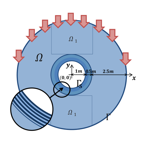


The quantity of interest is chosen to be the following
which represents the (rescaled, time-averaged) acoustic energy of the scattered wave concealed in the region (see Figure 1). For the considered parameter set is ranging from to , where at frequency .
The problem is symmetric with respect to the axis, therefore only half of the domain has to be considered for discretization. For the discretization, we used piecewise quadratic approximation on a mesh of triangular (finite) elements. The mesh was chosen such that there were at least degrees of freedom per wavelength, which is a standard choice for Helmholtz problems with a moderate wave number. It yielded approximately complex degrees of freedom for the discretization. Figures 1 to 1 depict the solutions for different parameter values with quantities of interest and , respectively.
It is revealed that for this problem, considering the classical inner product for the solution space leads to dramatic instabilities of the projection-based MOR methods. To improve the stability, the inner product is chosen corresponding to the specific structure of the operator in (53). The solution space is here equipped with the following inner product
| (54) |
where and are the functions identified with and , respectively, and and are the density and the wave number associated with the unperturbed cloak (i.e., with properties from Table 1) at frequency .
The operator for this benchmark is directly given in an affine form with terms. Furthermore, for online efficiency we used empirical interpolation method [33, 4] to obtain an approximate affine representation of (or rather a vector from representing an approximation of ) and the right hand side vector with affine terms (with error close to machine precision). The approximation space of dimension was constructed with a greedy algorithm (based on sketched minres projection) performed on a training set of uniform random samples in . The test set was taken as uniform random samples in .
Minimal residual projection. Let us first address the validation of the sketched minres projection from Section 3.2. For this we computed sketched (and standard) minres projections of onto for each with sketching matrix of varying sizes. The error of approximation is here characterized by and , where is the vector representing the incident wave and is the right hand side vector associated with the unperturbed cloak and the frequency (see Figures 2(a) and 2(c)). Furthermore, in Figure 2(e) we provide the characterization of the maximal error in the quantity of interest . For each size of , realizations of the sketching matrix were considered to analyze the statistical properties of , and .
For comparison, along with the minimal residual projections we also computed the sketched (and classical) Galerkin projection introduced in [3]. Figures 2(b), 2(d) and 2(f) depict the errors , , of a sketched (and classical) Galerkin projection using of different sizes. Again, for each we used realizations of to characterize the statistical properties of the error. We see that the classical Galerkin projection is more accurate in the exact norm and the quantity of interest than the standard minres projection. On the other hand, it is revealed that the minres projection is far better suited to random sketching.
From Figure 2 one can clearly report the (essential) preservation of the quality of the classical minres projection for . Note that for the minres projection a small deviation of and is observed. These errors are higher or lower than the standard values with (almost) equal probability (for ). In contrast to the minres projection, the quality of the Galerkin projection is not preserved even for large up to . This can be explained by the fact that the approximation of the Galerkin projection with random sketching is highly sensitive to the properties of the operator, which here is non-coercive and has a high condition number (for some parameter values), while the (essential) preservation of the accuracy of the standard minres projection by its sketched version is guaranteed regardless of the operator’s properties. One can clearly see that the sketched minres projection using with just rows yields better approximation (in terms of the maximal observed error) of the solution than the sketched Galerkin projection with , even though the standard minres projection is less accurate than the Galerkin one.
As already discussed, random sketching improves not only efficiency but also has an advantage of making the reduced model less sensitive to round-off errors thanks to possibility of direct online solution of the (sketched) least-squares problem without appealing to the normal equation. Figure 3 depicts the maximal condition number over of the reduced matrix associated with the sketched minres projection using reduced basis matrix with (approximately) unit-orthogonal columns with respect to , for varying sizes of . We also provide the maximal condition number of the reduced (normal) system of equations associated with the classical minres projection. It is observed that indeed random sketching yields an improvement of numerical stability by a square root.
Certification of the sketch. Next the experimental validation of the procedure for a posteriori certification of the -sketch or the sketched solution (see Section 5) is addressed. For this, we generated several of different sizes and for each of them computed the sketched minres projections for all . Thereafter Propositions 5.2 and 5.3, with defined by (17), were considered for certification of the residual error estimates or the quasi-optimality of in the residual error. Oblivious embeddings of varying sizes were tested for . For simplicity it was assumed that all considered satisfy (47) with and (small) probability of failure .
By Proposition 5.2 the certification of the sketched residual error estimator can be performed by comparing it to . More specifically, by (49) we have that with probability at least ,
| (55) |
Figure 4 depicts , where is the exact discrepancy or its (probabilistic) upper bound in (55). For each and , realizations of were computed for statistical analysis. We see that (sufficiently) tight upper bounds for were obtained already when , which is in particular several times smaller than the size of required for quasi-optimality of . This implies that the certification of the effectivity of the error estimator by should require negligible computational costs compared to the cost of obtaining the solution (or estimating the error in adaptive algorithms such as greedy algorithms).
By Proposition 3.3, the quasi-optimality of can be guaranteed if is an -embedding for . The -embedding property of each was verified with Proposition 5.3. In Figure 5 we provide where , which is the minimal value for such that is an -embedding for , or , which is the upper bound of computed with (51) using of varying sizes. For illustration purposes we here allow the value in Definition 2.1 to be larger than . The statistical properties of were obtained with realizations for each and value of . Figure 5(a) depicts the statistical characterization of for of size . The maximal value of observed for each and is presented in Figure 5(b). It is observed that with a posteriori estimates from Proposition 5.3 using of size , we here can guarantee with high probability that with satisfies an -embedding property for . The theoretical bounds from [3] for to be an -embedding for with yield much larger sizes, namely, for the probability of failure , they require more than rows for Gaussian matrices and rows for SRHT. This proves Proposition 5.3 to be very useful for the adaptive selection of sizes of random matrices or for the certification of the sketched inner product for all vectors in . Note that the adaptive selection of the size of can also be performed without requiring to be an -embedding for with , based on the observation that oblivious embeddings yield preservation of the quality of the minres projection when they are -embeddings for with small , which is possibly larger than (see Remark 6.1).
Remark 6.1.
Throughout the paper the quality of (e.g., for approximation of minres projection in Section 3.2) was characterized by -embedding property. However, for this numerical benchmark the sufficient size for to be an -embedding for is in several times larger than the one yielding an accurate approximation of the minres projection. In particular, with rows provides with high probability an approximation with residual error very close to the minimal one, but it does not satisfy an -embedding property (with ), which is required for guaranteeing the quasi-optimality of with Proposition 3.3. A more reliable way for certification of the quality of for approximation of the minres projection onto can be derived by taking into account that was generated from a distribution of oblivious embeddings. In such a case it is enough to only certify that provides an approximate upper bound of for all vectors in without the need to guarantee that is an approximate lower bound (that is in practice the main bottleneck). This approach is outlined below.
We first observe that was generated from a distribution of random matrices such that for all , we have
The values and can be obtained from the theoretical bounds from [3] or practical experience. Then one can show that for the sketched minres projection associated with , the inequality
| (56) |
holds with probability at least , where is the minimal value for such that for all
The quasi-optimality of in the norm rather than the residual norm can be readily derived from relation (56) by using the equivalence between the residual norm and the error in .
In this way a characterization of the quasi-optimality of the sketched minres projection with can be obtained from the a posteriori upper bound of in (56). Note that since is an oblivious subspace embedding, the parameters and do not depend on the dimension of , which implies that the considered value for should be an order of magnitude less than . Therefore, it can be a good way to choose as (or rather its upper bound) multiplied by a small factor, say .
The (probabilistic) upper bound for can be obtained a posteriori by following a similar procedure as the one from Proposition 5.3 described for verification of the -embedding property. More precisely, we can use similar arguments as in Proposition 5.3 to show that
is an upper bound for with probability at least .
Let us now provide experimental validation of the proposed approach. For this we considered same sketching matrices as in the previous experiment for validation of the -embedding property. For each we computed , where or its upper bound using of different sizes (see Figure 6). Again realizations of were considered for the statistical characterization of for each and size of . One can clearly see that the present approach provides better estimation of the quasi-optimality constants than the one with the -embedding property. In particular, the quasi-optimality guarantee for with rows is experimentally verified. Furthermore, we see that in all the experiments the a posteriori estimates are lower than even for of small sizes, yet they are larger than the exact values, which implies efficiency and robustnesses of the method. From Figure 6, a good accuracy of a posteriori estimates is with high probability attained for .
Computational costs. For this benchmark, random sketching yielded drastic computational savings in the offline stage and considerably improved online efficiency. To verify the gains for the offline stage, we executed two greedy algorithms for the generation of the reduced approximation space of dimension based on the minres projection and the sketched minres projection, respectively. The standard algorithm resulted in a computational burden after reaching -th iteration due to exceeding the limit of RAM (GB). This took more than hours of runtime. Note that performing iterations in this case would require around GB of RAM (mainly utilized for storage of the affine factors of ) and more than hours of runtime. In contrast to the standard method, conducting iterations of a greedy algorithm with random sketching using of size (and of size ) for the sketched minres projection and of size for the error certification, took only GB of RAM. Moreover, the sketch required only a minor part (GB) of the aforementioned amount of memory, while the major part was consumed by the initialization and maintenance of the full order model. The sketched greedy algorithm had a total runtime of hours, which is less than the (expected) runtime for the standard greedy algorithm in more than times. From these hours, hours was spent on computation of snapshots, hours on provisional online solutions and hours on random projections.
Next the improvement of online computational cost of minres projection is addressed. For this, we computed the reduced solutions on the test set with a standard method, which consists in assembling the reduced system of equations (representing the normal equation) from its affine decomposition (precomputed in the offline stage) and its subsequent solution with built in Matlab® R2017b linear solver. The online solutions on the test set were additionally computed with the sketched method for comparison of runtimes and storage requirements. For this, for each parameter value, the reduced least-squares problem was assembled from the precomputed affine decompositions of and and solved with the normal equation using the built in Matlab® R2017b linear solver. Note that both methods proceeded with the normal equation. The difference was in the way how this equation was obtained. For the standard method it was directly assembled from the affine representation, while for the sketched method it was computed from the sketched matrices and .
Table 2 depicts the runtimes and memory consumption taken by the standard and sketched minres online stages for varying sizes of the reduced space and (for the sketched method). The sketch’s sizes were picked such that the associated reduced solutions with high probability had almost (higher by at most a factor of ) optimal residual error. Our approach nearly divided by 3 the online runtime for all values of from Table 2. Furthermore, the improvement of memory requirements was even greater. For instance, for the online memory consumption was divided by . In Table 2 we also provide the cost of standard/sketched Galerkin online stage, which is more efficient than the other two due to less cost of forming the reduced system of equations (but can have worse quasi-optimality constants for non-coercive or ill-conditioned problems).
| Standard minres | Sketched minres | Galerkin | |||||||
|---|---|---|---|---|---|---|---|---|---|
| CPU | |||||||||
| Storage | |||||||||
6.2 Advection-diffusion problem
The dictionary-based approximation method proposed in Section 4 is validated on a D advection dominated advection-diffusion problem defined on a complex flow. This problem is governed by the following equations
| (57) |
where is the unknown (temperature) field, is the diffusion coefficient and is the advection field. The geometry of the problem is as follows. First we have circular pores of radius located at points , . The domain of interest is then defined as the square without the pores, i.e, , with . The boundaries and are taken as and , respectively. Furthermore, is (notationally) divided into the main region inside , and the outer domain playing a role of a boundary layer. Finally, the force term is nonzero in the disc . The geometric setup of the problem is presented in Figure 7.


The advection field is taken as a potential (divergence-free and curl-free) field consisting of a linear combination of components,
where
| (58) |
The vectors and are the basis vectors of the Cartesian system of coordinates. The vectors and are the basis vectors of the polar coordinate system with the origin at point , . From the physics perspective, we have here a superposition of two uniform flows and five hurricane flows (each consisting of a sink and a rotational flow) centered at different locations. The source term is
We consider a multi-objective scenario, where one aims to approximate the average solution field , , inside sensor having a form of a disc of radius located as in Figure 7. The objective is to obtain sensor outputs for the parameter values . Figures 7 to 7 present solutions for few samples from .
The discretization of the problem was performed with the classical finite element method. A nonuniform mesh was considered with finer elements near the pores of the hurricanes, and larger ones far from the pores such that each element’s Peclet number inside was larger than for any parameter value in . Moreover, it was revealed that for this benchmark the solution field outside the region was practically equal to zero for all . Therefore the outer region was discretized with coarse elements. For the discretization we used about and degrees of freedom in the main region and the outside boundary layer, respectively, which yielded approximately degrees of freedom in total.
The solution space is equipped with the inner product
that is the inner product for functions associated with vectors in .
For this problem, approximation of the solution with a fixed low-dimensional space is ineffective. The problem has to be approached with non-linear approximation methods with parameter-dependent approximation spaces. For this, the classical -refinement method is computationally intractable due to high dimensionality of the parameter domain, which makes the dictionary-based approximation to be the most pertinent choice.
The training and test sets and were respectively chosen as and uniform random samples from . Then, Algorithm 3 was employed to generate dictionaries of sizes , and for the dictionary-based approximation with , and vectors, respectively. For comparison, we also performed a greedy reduced basis algorithm (based on sketched minres projection) to generate a fixed reduced approximation space, which in particular coincides with Algorithm 3 with large enough (here ). Moreover, for more efficiency (to reduce the number of online solutions) at -th iteration of Algorithm 3 and reduced basis algorithm instead of taking as a maximizer of over , we relaxed the problem to finding any parameter-value such that
| (59) |
where denotes the solution obtained at the -th iteration. Note that (59) improved the efficiency, yet yielding at least as accurate maximizer of the dictionary-based width (defined in (24)) as considering . For the error certification purposes, each iterations the solution was computed on the whole training set and was taken as . Figure 8 depicts the observed evolutions of the errors in the greedy algorithms.
We see that at the first iterations, the error decay for the dictionary generation practically coincides with the error decay of the reduced basis algorithm, which can be explained by the fact that the first iterations of the two algorithms coincide. The convergence rates remain the same for the reduced basis algorithm (even at high iterations), while they slowly subsequently degrade for dictionary-based approximation. The latter method still highly outperforms the former one, since its online computational cost scales only linearly with the number of iterations. Furthermore, for the dictionary-based approximation the convergence of the error is moderately noisy. The noise is primarily due to approximating the solutions of online sparse least-squares problems with the orthogonal greedy algorithm, for which the accuracy can be sensitive to the enrichment of the dictionary with new vectors. The quality of online solutions could be improved by the usage of more sophisticated methods for sparse least-squares problems.
As it is clear from Figure 8, the obtained dictionaries and the bases taken from them provide approximations at least as accurate (on the training set) as the minres approximation with a fixed reduced space of dimension . Yet, the dictionary-based approximations are much more online-efficient. Table 3 provides the online complexity and storage requirements for obtaining the dictionary-based solutions for all (recall, ) with the orthogonal greedy algorithm (Algorithm 2) from a sketch of size , and the sketched minres solutions with QR factorization with Householder transformations (as in Matlab® R2017b least-squares solver) of the sketched reduced matrix in (20) from a sketch of size . In particular, we see that the dictionary-based approximation with and yields a gain in complexity by a factor of and memory consumption by a factor of . In Table 3 we also provide the associated runtimes and required RAM. It is revealed that the dictionary-based approximation with and had an about times speedup. The difference between the gains in terms of complexity and runtime can be explained by high efficiency of the Matlab® R2017b least-squares solver. It is important to note that even more considerable enhance of efficiency could be obtained by better exploitation of the structure of the dictionary-based reduced model, in particular, by representing the sketched matrix in a format well suited for the orthogonal greedy algorithm (e.g., a product of a dense matrix by several sparse matrices similarly as in [32, 38]).
| RB, | ||||
|---|---|---|---|---|
| Complexity in flops | ||||
| Storage in flns | ||||
| CPU in | ||||
| Storage in MB |
Further we provide statistical analysis of the dictionary-based approximation with and . For this we computed the associated dictionary-based solutions for all parameter values in the test set, considering of varying sizes. The accuracy of an approximation is characterized by the quantities , and , . Figure 9 depicts the dependence of , and (for few selected values of ) on the number of rows of . For each value of , the statistical properties of , and were characterized with realizations of , and . It is observed that for , the errors and are concentrated around and , respectively. Moreover, for all tested we obtained nearly the same errors, which suggests preservation of the quality of the dictionary-based approximation by its sketched version at . A (moderate) deviation of the errors in the quantities of interest (even for very large ) can be explained by (moderately) low effectivity of representation of these errors with the error in , which we considered to control.
7 Conclusion
In this article we have extended the methodology from [3] to minres methods and proposed a novel nonlinear approximation method to tackle problems with a slow decay of Kolmogorov -width. The main ingredient of our approach is the approximation of the reduced model’s solution from a random sketch, which entails drastic reduction of the computational costs and improvement of numerical stability. Precise conditions on the sketch to yield the (approximate) preservation of the quasi-optimality constants of the reduced model’s solution are provided. These conditions do not depend on the operator’s properties, which implies robustness for ill-conditioned and non-coercive problems. Moreover, these conditions can be ensured with SRHT or Gaussian matrices of sufficiently large sizes depending only logarithmically on the probability of failure and on the cardinality of the dictionary (for dictionary-based approximation).
We here also proposed efficient randomized methods for extraction of the quantity of interest (see Appendix A) and a posteriori certification of the reduced model’s sketch. These results along with the sketched minres projection can be used as a remedy of the drawbacks revealed in [3].
The applicability of the proposed methodology was realized on two benchmark problems difficult to tackle with standard methods. The experiments on the invisibility cloak benchmark confirmed that random sketching can indeed provide high computational savings in both offline and online stages, and more numerical stability compared to the standard minres method while preserving the quality of the output. It was illustrated experimentally that the random sketching technique may be better suited to minres methods than to Galerkin methods. Furthermore, the proposed procedure for the a posteriori certification of the sketch’s quality was also experimentally tested. It yielded bounds for the dimension of random projections an order of magnitude less than the theoretical ones from [3]. In the advection-diffusion benchmark a slow-decay of the Kolmogorov -width was revealed, which implied the necessity to use the dictionary-based approximation. It was verified that for this problem the dictionary-based approximation provided an enhancement of the online stage in more than an order of magnitude in complexity, in about times in terms of memory, and in about times in terms of runtime (compared to the sketched minres projection). Moreover, even higher computational savings could be obtained by representing the sketch of the dictionary in a more favorable format (e.g., as in [32, 38]), which we leave for future research.
References
- [1] D. Amsallem, C. Farhat, and M. Zahr. On the robustness of residual minimization for constructing pod-based reduced-order cfd models. 21st AIAA Computational Fluid Dynamics Conference, 2013.
- [2] D. Amsallem and B. Haasdonk. Pebl-rom: Projection-error based local reduced-order models. Advanced Modeling and Simulation in Engineering Sciences, 3(1):6, 2016.
- [3] O. Balabanov and A. Nouy. Randomized linear algebra for model reduction. Part I: Galerkin methods and error estimation. Advances in Computational Mathematics 45:2969–3019, 2019.
- [4] M. Barrault, Y. Maday, N. C. Nguyen, and A. T. Patera. An empirical interpolation method: application to efficient reduced-basis discretization of partial differential equations. Comptes Rendus Mathématique, 339(9):667–672, 2004.
- [5] P. Benner, A. Cohen, M. Ohlberger, and K. Willcox, editors. Model Reduction and Approximation: Theory and Algorithms. SIAM, Philadelphia, PA, 2017.
- [6] K. Bertoldi, V. Vitelli, J. Christensen, and M. van Hecke. Flexible mechanical metamaterials. Nature Reviews Materials, 2(11):17066, 2017.
- [7] D. A. Bistrian and I. M. Navon. Randomized dynamic mode decomposition for nonintrusive reduced order modelling. International Journal for Numerical Methods in Engineering, 112(1):3–25, 2017.
- [8] S. L. Brunton, J. L. Proctor, J. H. Tu, and J. N. Kutz. Compressed sensing and dynamic mode decomposition. Journal of Computational Dynamics, 2:165, 2015.
- [9] A. Buhr and K. Smetana. Randomized local model order reduction. SIAM Journal on Scientific Computing, 40:2120–2151, 2018.
- [10] T. Bui-Thanh, K. Willcox, and O. Ghattas. Model reduction for large-scale systems with high-dimensional parametric input space. SIAM Journal on Scientific Computing, 30(6):3270–3288, 2008.
- [11] Y. Cao and L. Petzold. A posteriori error estimation and global error control for ordinary differential equations by the adjoint method. SIAM Journal on Scientific Computing, 26(2):359–374, 2004.
- [12] K. Carlberg, L. Farhat, J., Cortial, and D., Amsallem. The GNAT method for nonlinear model reduction: effective implementation and application to computational fluid dynamics and turbulent flows. Journal of Computational Physics, 242:623–647, 2013.
- [13] H. Chen and C. T. Chan. Acoustic cloaking and transformation acoustics. Journal of Physics D: Applied Physics, 43(11):113001, 2010.
- [14] Y. Chen, J. S. Hesthaven, Y. Maday, and J. Rodríguez. A monotonic evaluation of lower bounds for inf-sup stability constants in the frame of reduced basis approximations. Comptes Rendus Mathematique, 346(23):1295 – 1300, 2008.
- [15] Y. Chen, J. S. Hesthaven, Y. Maday, and J. Rodríguez. Improved successive constraint method based a posteriori error estimate for reduced basis approximation of 2D Maxwell’s problem. ESAIM: Mathematical Modelling and Numerical Analysis, 43(6):1099–1116, 2009.
- [16] Y. Cheng, F. Yang, J. Y. Xu, and X. J. Liu. A multilayer structured acoustic cloak with homogeneous isotropic materials. Applied Physics Letters, 92(15):151913, 2008.
- [17] R. A. DeVore. Nonlinear approximation and its applications. In Multiscale, Nonlinear and Adaptive Approximation, pages 169–201. Springer, 2009.
- [18] M. Dihlmann, S. Kaulmann, and B. Haasdonk. Online reduced basis construction procedure for model reduction of parametrized evolution systems. IFAC Proceedings Volumes, 45(2):112–117, 2012.
- [19] J. L. Eftang, D. J. Knezevic, and A. T. Patera. An hp certified reduced basis method for parametrized parabolic partial differential equations. Mathematical and Computer Modelling of Dynamical Systems, 17(4):395–422, 2011.
- [20] J. L. Eftang, A. T. Patera, and E. M. Rønquist. An ”hp” certified reduced basis method for parametrized elliptic partial differential equations. SIAM Journal on Scientific Computing, 32(6):3170–3200, 2010.
- [21] N. B. Erichson and C. Donovan. Randomized low-rank dynamic mode decomposition for motion detection. Computer Vision and Image Understanding, 146:40–50, 2016.
- [22] N. B. Erichson, L. Mathelin, S. L. Brunton, and J. N. Kutz. Randomized dynamic mode decomposition. SIAM Journal on Applied Dynamical Systems, 18(4):1867–1891, 2019.
- [23] B. Haasdonk. Reduced basis methods for parametrized PDEs – A tutorial introduction for stationary and instationary problems. Model reduction and approximation: theory and algorithms, 15:65, 2017.
- [24] N. Halko, P.-G. Martinsson, and J. A. Tropp. Finding structure with randomness: Probabilistic algorithms for constructing approximate matrix decompositions. SIAM review, 53(2):217–288, 2011.
- [25] A. Hochman, J. F. Villena, A. G. Polimeridis, L. M. Silveira, J. K. White, and L. Daniel. Reduced-order models for electromagnetic scattering problems. IEEE Transactions on Antennas and Propagation, 62(6):3150–3162, 2014.
- [26] C. Homescu, L. R. Petzold, and R. Serban. Error estimation for reduced-order models of dynamical systems. SIAM Journal on Numerical Analysis, 43(4):1693–1714, 2005.
- [27] D. B. P. Huynh, G. Rozza, S. Sen, and A. T. Patera. A successive constraint linear optimization method for lower bounds of parametric coercivity and inf–sup stability constants. Comptes Rendus Mathématique, 345(8):473–478, 2007.
- [28] D. B. P. Huynh, D. J. Knezevic, Y. Chen, J. S. Hesthaven and A. T. Patera. A natural-norm Successive Constraint Method for inf-sup lower bounds. Computer Methods in Applied Mechanics and Engineering, 199(29):1963 – 1975, 2010.
- [29] M. Kadic, T. Bückmann, R. Schittny, P. Gumbsch, and M. Wegener. Pentamode metamaterials with independently tailored bulk modulus and mass density. Physical Review Applied, 2(5):054007, 2014.
- [30] S. Kaulmann and B. Haasdonk. Online greedy reduced basis construction using dictionaries. In VI International Conference on Adaptive Modeling and Simulation (ADMOS 2013), pages 365–376, 2013.
- [31] B. Kramer, P. Grover, P. Boufounos, S. Nabi, and M. Benosman. Sparse sensing and dmd-based identification of flow regimes and bifurcations in complex flows. SIAM Journal on Applied Dynamical Systems, 16(2):1164–1196, 2017.
- [32] L. Le Magoarou and R. Gribonval. Flexible multilayer sparse approximations of matrices and applications. IEEE Journal of Selected Topics in Signal Processing, 10(4):688–700, 2016.
- [33] Y. Maday, N. C. Nguyen, A. T. Patera, and S. H. Pau. A general multipurpose interpolation procedure: the magic points. Communications on Pure & Applied Analysis, 8(1):383, 2009.
- [34] Y. Maday and B. Stamm. Locally adaptive greedy approximations for anisotropic parameter reduced basis spaces. SIAM Journal on Scientific Computing, 35(6):2417–2441, 2013.
- [35] M. W. Mahoney et al. Randomized algorithms for matrices and data. Foundations and Trends® in Machine Learning, 3(2):123–224, 2011.
- [36] V. Rokhlin and M. Tygert. A fast randomized algorithm for overdetermined linear least-squares regression. Proceedings of the National Academy of Sciences, 105(36):13212–13217, 2008.
- [37] G. Rozza, D. B. P. Huynh, A. T. Patera. Reduced basis approximation and a posteriori error estimation for affinely parametrized elliptic coercive partial differential equations. Archives of Computational Methods in Engineering, 15(3):1, 2007.
- [38] R. Rubinstein, M. Zibulevsky, and M. Elad. Double sparsity: Learning sparse dictionaries for sparse signal approximation. IEEE Transactions on signal processing, 58(3):1553–1564, 2009.
- [39] K. Smetana, O. Zahm, and A. T. Patera. Randomized residual-based error estimators for parametrized equations. SIAM journal on scientific computing, 41(2):900–926, 2019.
- [40] T. Taddei. An offline/online procedure for dual norm calculations of parameterized functionals: empirical quadrature and empirical test spaces. Advances in Computational Mathematics 45(5-6):2429–2462, 2019.
- [41] V. N. Temlyakov. Nonlinear Kolmogorov widths. Mathematical Notes, 63(6):785–795, 1998.
- [42] J. A. Tropp and A. C. Gilbert. Signal recovery from random measurements via orthogonal matching pursuit. IEEE Transactions on information theory, 53(12):4655–4666, 2007.
- [43] D. P. Woodruff et al. Sketching as a tool for numerical linear algebra. Foundations and Trends® in Theoretical Computer Science, 10(1–2):1–157, 2014.
- [44] O. Zahm and A. Nouy. Interpolation of inverse operators for preconditioning parameter-dependent equations. SIAM Journal on Scientific Computing, 38(2):1044–1074, 2016.
Appendix A. Post-processing the reduced model’s solution
In the paper we presented a methodology for efficient computation of an approximate solution , or to be more precise, its coordinates in a certain basis, which can be the classical reduced basis for a fixed approximation space, or the dictionary vectors for dictionary-based approximation presented in Section 4. The approximate solution , however, is usually not what one should consider as the output. In fact, the amount of allowed online computations is highly limited and should be independent of the dimension of the full order model. Therefore outputting bytes of data as should be avoided when is not the quantity of interest.
Further, we shall consider an approximation with a single subspace noting that the presented approach can also be used for post-processing the dictionary-based approximation from Section 4 (by taking as the subspace spanned by the dictionary vectors). Let be a matrix whose column vectors form a basis for and let be the coordinates of in this basis. A general quantity of interest can be approximated by . Further, let us assume a linear case where with being the extractor of the quantity of interest. Then
| (60) |
where .
Remark 8.1.
In general, our approach can be used for estimating an inner product between arbitrary parameter-dependent vectors. The possible applications include efficient estimation of the primal-dual correction and an extension to quadratic quantities of interest. In particular, the estimation of the primal-dual correction can be obtained by replacing by and by in (60), where is a reduced basis (or dictionary-based) approximate solution to the adjoint problem. A quadratic output quantity of interest has the form , where and . Such can be readily derived from (60) by replacing with .
The affine factors of should be first precomputed in the offline stage and then used for online evaluation of for each parameter value with a computational cost independent of the dimension of the original problem. The offline computations required for evaluating the affine factors of , however, can still be too expensive or even unfeasible to perform. Such a scenario may arise when using a high-dimensional approximation space (or a dictionary), when the extractor has many (possibly expensive to maintain) affine terms, or when working in an extreme computational environment, e.g., with data streamed or distributed among multiple workstations. In addition, evaluating from the affine expansion as well as evaluating itself can be subject to round-off errors (especially when is ill-conditioned and may not be orthogonalized). Further, we shall provide a (probabilistic) way for estimating with a reduced computational cost and better numerical stability. As the core we take the idea from [3, Section 4.3] proposed as a workaround to expensive offline computations for the evaluation of the primal-dual correction.
Remark 8.2.
The spaces and are equipped with inner products and (defined by matrix ), which are used for controlling the accuracy of the approximate solution . In general, is chosen according to both the operator and the extractor of the quantity of interest. The goal of this section, however, is only the estimation of the quantity of interest from the given . Consequently, for many problems it can be more pertinent to use here a different than the one employed for obtaining and characterizing . The choice for should be done according to (independently of ). For instance, for discretized parametric PDEs, if represents an integral of the solution field over the spatial domain then it is natural to choose corresponding to the inner product. Moreover, is required to be an inner product only on a certain subspace of interest, which means that may be a positive semi-definite matrix. This consideration can be particularly helpful when the quantity of interest depends only on the restriction of the solution field to a certain subdomain. In such a case, can be chosen to correspond with an inner product between restrictions of functions to this subdomain. The extension of random sketching for estimation of semi-inner products is straightforward (see Remark 8.3).
Remark 8.3.
Let us outline the extension of the methodology to the case where is not definite. Let us assume that is an inner product on a subspace of interest. Then, it follows that can be equipped with , where is a pseudo-inverse of . Such products and can be approximated by
| (61) |
This can be useful for the estimation of a (semi-)inner product between parameter-dependent vectors (see Remark 8.2).
8.1 Approximation of the quantity of interest
An efficiently computable and accurate estimation of can be obtained in two phases. In the first phase, the manifold is (accurately enough) approximated with a subspace , which is spanned by an efficient to multiply (i.e., sparse or low-dimensional) matrix . This matrix can be selected a priori or obtained depending on . In Section 8.2 we shall provide some strategies for choosing or computing the columns for . The appropriate strategy should be selected depending on the particular problem and computational architecture. Further, the solution vector is approximated by its orthogonal projection on . The coordinates can be obtained from by
| (62) |
where . Note that since is efficient to multiply by, the matrix can be efficiently precomputed in the offline stage. We arrive at the following estimation of :
| (63) |
where . Unlike , the affine factors of can now be efficiently precomputed thanks to the structure of .
In the second phase of the algorithm, the precision of (63) is improved with a sketched (random) correction associated with an subspace embedding :
| (64) |
In practice, can be efficiently evaluated using the following relation:
| (65) |
where the affine terms of can be precomputed from the -sketch of , a sketched matrix and the matrix with a negligible computational cost.
Proposition 8.4.
If is an oblivious subspace embedding,
| (66) |
holds for a fixed parameter with probability at least .
Proposition 8.5.
Let denote a subspace containing . If is an -embedding for , then (66) holds for all .
It follows that the accuracy of can be controlled through the quality of for approximating , the quality of as an -embedding, or both. Note that choosing as a null matrix (i.e., an -embedding for with ) leads to a single first-phase approximation (63), while letting corresponds to a single sketched (second-phase) approximation. Such particular choices for or can be pertinent when the subspace is highly accurate so that there is practically no benefit to use a sketched correction or, the other way around, when the computational environment or the problem does not permit a sufficiently accurate approximation of with , therefore making the use of a non-zero unjustified.
Remark 8.6.
When interpreting random sketching as a Monte Carlo method for the estimation of the inner product , the proposed approach can be interpreted as a control variate method where plays the role of the control variate. A multileveled Monte Carlo method with different control variates should further improve the efficiency of post-processing.
8.2 Construction of reduced subspaces
Further we address the problem of computing the basis vectors for . In general, the strategy for obtaining has to be chosen according to the problem’s structure and the constraints due to the computational environment.
A simple way, used in [3], is to choose as the span of samples of either chosen randomly or during the first few iterations of the reduced basis (or dictionary) generation with a greedy algorithm. Such , however, may be too costly to operate with. Then we propose more sophisticated constructions of .
Approximate Proper Orthogonal Decomposition. A subspace can be obtained by an (approximate) POD of the reduced vectors evaluated on a training set . Here, randomized linear algebra can be again employed for improving efficiency. The computational cost of the proposed POD procedure shall mainly consist of the solution of reduced problems and the multiplication of by small vectors. Unlike the classical POD, our methodology does not require computation or maintenance of the full solution’s samples and therefore allows large training sets.
Let be a training sample of the coordinates of in a basis . We look for a POD subspace associated with the snapshot matrix
where is a matrix whose columns are the elements from .
An accurate estimation of POD can be efficiently computed via the sketched method of snapshots introduced in [3, Section 5.2]. More specifically, a quasi-optimal (with high probability) POD basis can be calculated as
| (67) |
where
with being the dominant singular vectors of . Note that the matrix can be efficiently obtained with a computational cost independent of the dimension of the full order model. The dominant cost is the multiplication of by , which is also expected to be inexpensive since has a small number of columns. Guarantees for the quasi-optimality of can be readily derived from [3, Theorem 5.5].
Sketched greedy algorithm. A greedy search over the training set of approximate solutions is another way to construct . At the -th iteration, is enriched with a vector with the largest distance to over the training set. Note that in this case the resulting matrix has the form (67), where . The efficiency of the greedy selection can be improved by employing random sketching technique. At each iteration, the distance to can be measured with the sketched norm , which can be computed from sketches of the approximate solutions with no need to operate with large matrix but only its sketch. This allows efficient computation of the quasi-optimal interpolation points and the associated matrix . Note that for numerical stability an orthogonalization of with respect to can be performed, that can be done by modifying so that is an orthogonal matrix. Such can be obtained with standard QR factorization. When has been computed, the matrix can be calculated by multiplying with . The quasi-optimality of and approximate orthogonality of is guaranteed if is an -embedding for all subspaces from the set . This property of can be guaranteed a priori by considering oblivious subspace embeddings, or certified a posteriori with the procedure explained in Section 5.
Coarse approximation. Let us notice that the online cost of evaluating does not depend on the dimension of . Consequently, if is spanned by structured (e.g., sparse) basis vectors then a rather high dimension is allowed (possibly larger than ).
For classical numerical methods for PDEs, the resolution of the mesh (or grid) is usually chosen to guarantee both an approximability of the solution manifold by the approximation space and the stability. For many problems the latter factor is dominant and one choses the mesh primary to it. This is a typical situation for wave problems, advection-diffusion-reaction problems and many others. For these problems, the resolution of the mesh can be much higher than needed for the estimation of the quantity of interest from the given solution field. In these cases, the quantity of interest can be efficiently yet accurately approximated using a coarse-grid interpolation of the solution.
Suppose that each vector represents a function in a finite-dimensional approximation space spanned by basis functions associated with a fine mesh of . The function can be approximated by a projection on a coarse-grid approximation space spanned by basis functions . For simplicity assume that each . Then the -th basis vector for can be obtained simply by evaluating the coordinates of in the basis . Note that for the classical finite element approximation, each basis function has a local support and the resulting matrix is sparse.
8.3 Numerical validation
The proposed methodology was validated experimentally on an invisibility cloak benchmark from Section 6.1.
As in Section 6.1 in this experiment we used an approximation space of dimension constructed with a greedy algorithm (based on sketched minres projection). We used a training set of uniform random samples in , while the test set was taken as uniform random samples in . The experiment was performed for a fixed approximation obtained with sketched minres projection on using with rows. For such , an approximate extraction of the quantity from (represented by coordinates in reduced basis) was considered.
The post-processing procedure was performed by choosing and in (60) as . Furthermore, for better accuracy the solution space was here equipped with (semi-)inner product that is different from the inner product (54) considered for ensuring quasi-optimality of the minres projection and error estimation (see Remark 8.2). For such choices of and , we employed a greedy search with error indicator over training set of uniform samples in to find . Then was efficiently approximated by given in (65). In this experiment, the error is characterized by , where or . The statistical properties of for each value of and were obtained with realizations of . Figure 10(a) exhibits the dependence of on the size of with of dimension . Furthermore, in Figure 10(b) we provide the maximum value from the computed samples for different sizes of and . The accuracy of can be controlled by the quality of for the approximation of and the quality of for the approximation of . When approximates well , one can use a random correction with of rather small size, while in the alternative scenario the usage of a large random sketch is required. In this experiment we see that the quality of the output is nearly preserved with high probability when using of dimension and a sketch of size , or of dimension and a sketch of size . For less accurate , with , the preservation of the quality of the output requires larger sketches of sizes . For optimizing efficiency the dimension for and the size for should be picked depending on the dimensions and of and , respectively, and the particular computational architecture. The increase of the considered dimension of entails storage and operation with more high-dimensional vectors, while the increase of the sketch entails higher computational cost associated with storage and operation with the sketched matrix . Let us finally note that for this benchmark the approximate extraction of the quantity of interest with our approach using and a sketch of size , required in about times less amount of storage and complexity than the classical exact extraction.
Appendix B. Proofs of propositions.
Proof of Proposition 3.1.
The statement of the proposition follows directly from the definitions of the constants and , that imply
∎
Proof of Proposition 3.3.
Proof of Proposition 3.5.
Let and . Then
Since is an -embedding for , we have
The statement of the proposition follows immediately. ∎
Proof of Proposition 4.1.
Take arbitrary , and let be dictionaries with , such that
The existence of follows directly from the definition (24) of the dictionary-based width. Define Then the following relations hold:
Since the above relations hold for arbitrary positive , we conclude that
∎
Proof of Proposition 4.3.
Let . By definition of and constants and ,
which ends the proof. ∎
Proof of Proposition 4.4.
The proof exactly follows the one of Proposition 4.3 by replacing with . ∎
Proof of Proposition 4.5.
We have that
holds for all with . The statement of the proposition then follows directly from the definitions of and . ∎
Proof of Proposition 4.6.
Let matrix have columns and matrix have columns , with being a subset of indices. Let be an arbitrary vector. Define a sparse vector with and zeros elsewhere. Let . Then
Similarly,
The statement of the proposition follows immediately. ∎
Proof of Proposition 5.2.
Proof of Proposition 5.3.
Observe that
Let us make the following assumption:
For the alternative case the proof is similar.
Next, we show that is an upper bound for with probability at least . Define . By definition of ,
| (72) |
holds with probability at least . If (72) is satisfied, we have
∎
Proof of Proposition 5.4.
By definition of and the assumption on , for all , it holds
The above relations and the definition (50) of yield
which ends the proof. ∎
Proof of Proposition 8.4.
Denote and . Let us consider , which also accounts for the real case, . Let
Observe that and is a real number.
By a union bound for the probability of success, is an -embedding for and with probability at least . Then, using the parallelogram identity we obtain
We conclude that relation (66) holds with probability at least . ∎