Fixation in Competing Populations: Diffusion and Strategies for Survival

Note that because the birth-rate and death-rate in FVMD are the same, the mean field equation for VMD and FVMD are identical. The equations for the concentration of $A$ and $B$ species are:

Using the above equations for $c_{A}$ and $c_{B}$, we obtain the following equations $c$ and $f$:

For $D_{A}=D_{B}$, Eq. (7) reduces to the Fisher equation Fisher1937; Kolmogorov1937.

For the CLVMD, we set $\gamma_{1}=\gamma_{2}=\gamma$ and obtain the following reaction-diffusion equations:

Again, from the above equations we get the following equations for the evolution of $c$ and $f$:

The homogeneous stable solution for the concentration equation is $c=\mu/\gamma$. Around this homogenous initial state, it is easy to see that the equations for CLVMD and VMD model are identical.

We focus on the fixation probability $\mathcal{F}$ which is the likelihood that a certain species would prevail over the other, and ask for the dispersal strategy which would maximize $\mathcal{F}$. Here is a summary of our main results (i) In the VMD where the total number of individuals is strictly conserved, $\mathcal{F}$ is invariant with respect to change in diffusivity irrespective of selective advantage. Thus in this case the variation of dispersal rate is ineffective as a strategy. (ii) In the FVMD, birth and death lead to fluctuations of the total number of individuals. In the neutral case ($s=0$), $\mathcal{F}$ remains independent of diffusivity. However, a new effect arises when $s\neq 0$: the optimal strategy for disadvantaged individuals is then to move slower. (iii) In the CLVMD, number fluctuations due to intra-species competition dominate; the best strategy to enhance $\mathcal{F}$ is then to move faster. In a nutshell, dispersal strategies become crucial in the presence of number fluctuations; but exactly what the optimal strategy is depends on the form of non-conservation. Below we present details of our investigation which lead to these conclusions and also remark on the fixation times for each species in the neutral case.

An important point is that the mean-field descriptions of the three models are similar, as shown in Eqs. 7, 11. Therefore for investigating the non-trivial effects that we highlighted in the introduction, we performed agent-based simulations for the models, supplement these by analytic arguments to support the numerical results.

In our numerical simulations, we start with $N/2$ individuals of type $A$ and an equal number of type $B$, placed randomly on a $1D$ lattice with $L$ sites with $N>L$. Thus the average density of individuals $\rho_{0}=N/L>1$. In each of the three models of population dynamics under study, there are two physical processes (i) reactions, namely birth, death, intra- and inter-species competition, and (ii) movement of individuals via diffusion. In our lattice model, reactions are on-site processes and diffusive moves happen between nearest-neighbour lattice sites. We split the reaction and diffusion processes, i.e., only reactions occur for a time interval $\Delta t$, followed by only diffusive moves for time $\Delta t$. The time interval $\Delta t$ is chosen to be much smaller than one Monte-Carlo step yet large enough that many reactions occur in $\Delta t$.

For reactions, we implement the event-based Gillespie algorithm Gillespie2007_1 at each site. To do so, we first calculate the propensity of all possible reactions on that site. A particular reaction would occur with a probability that is proportional to its rate. Let us consider a site $i$ containing $n_{A}$ individuals of type $A$ and $n_{B}$ number of type $B$. At this site, the total number of possible reactions due to birth, death, intra-species and inter-species reactions is

We choose $\mu^{A}_{birth}=\mu^{B}_{birth}=\mu^{A}_{death}=\mu^{B}_{death}=\mu$ in our numerical simulation. The probability of a particular reaction event occurring is the ratio of the rate of the event to the total rate $\mathcal{R}$. For instance, $A$ would become $2A$ with probability $\frac{\mu\,n_{A}}{\mathcal{R}}$. If the reaction happens, the next step is to increase the time by $\ln(1/r)/\mathcal{R}$ where $r\in(0,1]$ is a random number chosen from uniform distribution. The number of $A$’s and $B$’s change after each successive reaction, thereby affecting the total rate $\mathcal{R}$ at the site. Quite a few reactions occur until the sum of the reaction time-steps just crosses the chosen $\Delta t$. We follow the same procedure for all other sites. Recall that during this time step $\Delta t$, we solely do the reaction, and inter-site diffusive hops are not allowed.

Once the reactions are completed on every site of the system up to time $\Delta t$, we move a randomly chosen set of $ND\Delta t$ individuals to one of the nearest neighbor sites, where $D$ is the hopping rate of the species. The time evolution is averaged over a number $N_{hist}$ of histories, each starting from a new initial condition, a typical value of $N_{hist}$ being $30,000$.

Numerical simulations show that the variation of $\mathcal{F}_{B}(0,\Delta D)$ with $\Delta D$ is quite different for the three models (Fig.  2). While $\mathcal{F}_{B}$ is immune to changing $\Delta D$ for the VMD and FVMD, it is very sensitive to $\Delta D$ for the CLVMD. These pronounced differences occur even though the mean-field equations for the concentration of species are the same for all three models.

VMD: The full dynamics involves diffusion with unequal $A$ and $B$ diffusivities along with $A$$-$$B$ symmetric reaction kinetics. The result of each reaction step is $2A$ or $2B$ with equal probability, implying that the overall numbers of $A$ and $B$ particles follow a Moran process. Thus $\mathcal{F}_{A}(0,\Delta D)=\mathcal{F}_{B}(0,\Delta D)=1/2$.

To understand the fixation dynamics, let us consider the case where $D_{A}=D$ and $D_{B}=0$. Starting from uniformly distributed $A$ and $B$ particles, very quickly isolated pillars with a large number of $B$-particles are formed (see Fig. 1(a) and (b) (bottom-left)). Consequently, the $A$ particle concentration in the vicinity of the pillar is strongly depleted. Furthermore, because of number fluctuations, with finite probability the local pillar can eventually convert quickly into all $A$’s. This leads to an increased local concentration of $A$, which then diffuse away as in Fig. 1(bottom-left). We have verified that this effect persists even when $D_{B}$ is nonzero, so long as $\Delta D>0$.

We observe that the mean fixation times for the species satisfy $\langle t_{A}\rangle<\langle t_{B}\rangle$ (see Table 1). First consider the case where $B$ fixates. At long times, we observe a single $B$ pillar with few scattered $A$ particles (see Fig. 1(b)). The scenario is exactly opposite for the case of $A$-fixation, where the last $B$ pillar is in a sea of a large number of $A$ particles (see Fig. 1). Thus the frequency of reaction in the latter case is larger than for $B$-fixation.

It is possible to obtain analytic results for the fixation probability as well as mean fixation times $\langle t_{A}\rangle$ and $\langle t_{B}\rangle$ in the limit of VMD dynamics in which one species (say $B$) has zero diffusivity, and the reactions happen infinitely fast. Consider the neutral case with an initial condition with $N_{0}=N/2$ $B$’s at a single site $S_{0}$ and no $A$ particles. At each time step, a single $A$ particle is assumed to reach $S_{0}$, on-site reactions being completed before the next $A$ arrives. We now show that the fixation probability $=1/2$ for both species, while mean times $\langle t_{A}\rangle$ and $\langle t_{B}\rangle$ for $A$ and $B$ fixation satisfy $\langle t_{A}\rangle<\langle t_{B}\rangle$.

Let us compute the probability $P_{A}(n)$ that global $A$ fixation occurs at the $n$’th step. $A$ particles arriving earlier at site $S_{0}$ must have converted to $B$, so that the number of $B$ particles after the $(n-1)$th step is $N_{0}+n-1$. The probability $Q(n-1)$ of this event is $g_{0}\times g_{1}\cdot\cdot\cdot\times g_{n-1}$ where $g_{i}=(N_{0}+i)/(N_{0}+i+1)$ is the probability that an $A$ particle arriving at the $i$’th step is converted to $B$. Thus $Q(n-1)=N_{0}/(N_{0}+n-1)$. Now consider the arrival of the next $A$ particle. The probability that reactions result in the $N_{0}+n$ particles becoming all $A$’s is then $1/(N_{0}+n)$. If this happens, the system would fixate globally to all $A$’s. Thus the probability $P_{A}(n)$ that $A$ fixation happens at the $n$’th time step is $Q(n-1)\times 1/(N_{0}+n)$. The overall $A$ fixation probability is then $\sum_{n=1}^{N_{0}}P_{A}(n)=1/2$, and the mean time of $A$ fixation is straightforwardly found to be

where $H(M)=\sum^{M}_{m=1}\frac{1}{m}$. For large $N_{0}$, it then follows that $\langle t_{A}\rangle\approx CN_{0}$ with $C=(2\,ln2-1)\approx 0.386N_{0}$.

On the other hand, in order for $B$ fixation to occur, the $B$’s must have survived at each of the earlier steps. The corresponding probability is $Q(N_{0})=\frac{1}{2}$, and the corresponding survival time is $\langle t_{B}\rangle=N_{0}$. Evidently, $\langle t_{A}\rangle<\langle t_{B}\rangle$ holds. This result accords with the qualitative point that the faster species fixates earlier on average.

FVMD: All reaction steps, whether interspecies competition or individual births or deaths, continue to maintain $A$$-$$B$ symmetry even if $\Delta D\neq 0$, as for the VMD. Thus inclusion of birth-death fluctuations in the FVMD thus does not change the conclusion $\mathcal{F}_{A}(0,\Delta D)=\mathcal{F}_{B}(0,\Delta D)=1/2$. For the same reason as VMD, the inequality $\langle t_{A}\rangle<\langle t_{B}\rangle$ (see Table 1) continues to hold for the FVMD.

CLVMD: An advantage for the faster species results from a combination of unequal diffusivities and intra-species death terms (Eq. (3)), which act on several particles of the same species on the same site. Consider first the $A$ particles. Owing to the faster $A$ diffusivity, $A$-particle concentration fluctuations spread out quickly, thus minimizing the effects of intra-species death. Dispersal of $B$ particles is slower, so fluctuations which lead to $B$ particle clustering decay relatively slowly. This makes $B$ particles more prone to intra-species death. A depleted $B$ population on a given site is then easier to convert to all $A$’s on that site through the competitive $A$ $-$ $B$ conversion terms (see Eq. (3)) pigo13. Thus overall, the optimal strategy to maximize the fixation probability within the CLVMD is to move fast.

We observe that $\langle t_{A}\rangle>\langle t_{B}\rangle$ holds for relatively small $L$, but the difference narrows down as $L$ increases (see Table 1). In the minority of cases in which the $B$ species does achieve fixation, it must be before the intra-species terms have had much effect. Thus $B$ fixation occurs at relatively early times.

Going beyond the neutral case, in order to study the change of fixation probability brought in by unequal diffusivity, we define

with $\Delta\mathcal{F}_{A}$ being defined similarly. Evidently we have $\Delta\mathcal{F}_{A}+\Delta\mathcal{F}_{B}=0$. Below, we see how $\Delta\mathcal{F}_{A,B}$ behaves in the three models under study.

VMD: The argument used in the neutral case applies also when $s\neq 0$, implying that the fixation probability is the same as that of the Moran process with the corresponding value of $s$. The outcome of a particular Moran step does not depend on the manner in which an $A$ and a $B$ reach the same site (Fig. 3). Hence $\Delta\mathcal{F}_{A}=\Delta\mathcal{F}_{B}=0.$

FVMD: The inclusion of birth-death processes has a strong effect and the best dispersal strategy now depends on the strength of the species. For instance, if $s>0$, then moving slowly is a better strategy than moving fast for the weaker $B$ species. Evidence for this comes from Fig. 4 which shows that $\Delta\mathcal{F}_{B}$ is positive when $\Delta D$ and $s$ are both positive. To see how birth-death fluctuations can affect fixation, refer to Fig. 3 which compares the sequence of events with $D_{B}=D_{A}$ and $D_{B}<D_{A}$. The separation $R$ between an $A$ and $B$ particle undergoes a random walk with an effective diffusion constant $D_{eff}=D_{A}+D_{B}=2D-\Delta D$. Thus, provided they survive, the typical time for the particles to meet is $\tau_{diff}\approx R^{2}/D_{eff}$. Further, owing to the birth-death process, the typical time of survival of an $A$ particle is $1/\mu$, implying there is a probability $(1-e^{-\mu\,\tau_{diff}})$ that the $A$ particle would not survive for time $\tau_{diff}$. Thus the best strategy for the weaker particle $B$ to survive is to increase $\tau_{diff}$ (decrease $D_{eff}$) to the maximum extent possible, which it can do by setting $D_{B}=0$, i.e., by standing still. This is corroborated by Fig.  4, which shows that $\Delta\mathcal{F}_{B}$ is positive for $s>0$ meaning that the disadvantage for the $B$ species is reduced. The accrued advantage increases with $s$ for small $s$. As $s$ increases in magnitude, selective advantage effects override the effects of unequal diffusivities, hence $\Delta{\mathcal{F}}_{B}\to 0$ as $|s|$ becomes large. This leads to the extrema in Fig. 4(a). In addition, we checked that our results do not depend on $\Delta t$ by varying a factor $4$,  and found that there is no appreciable change in our numerical estimates of the fixation probability (Fig. 5).

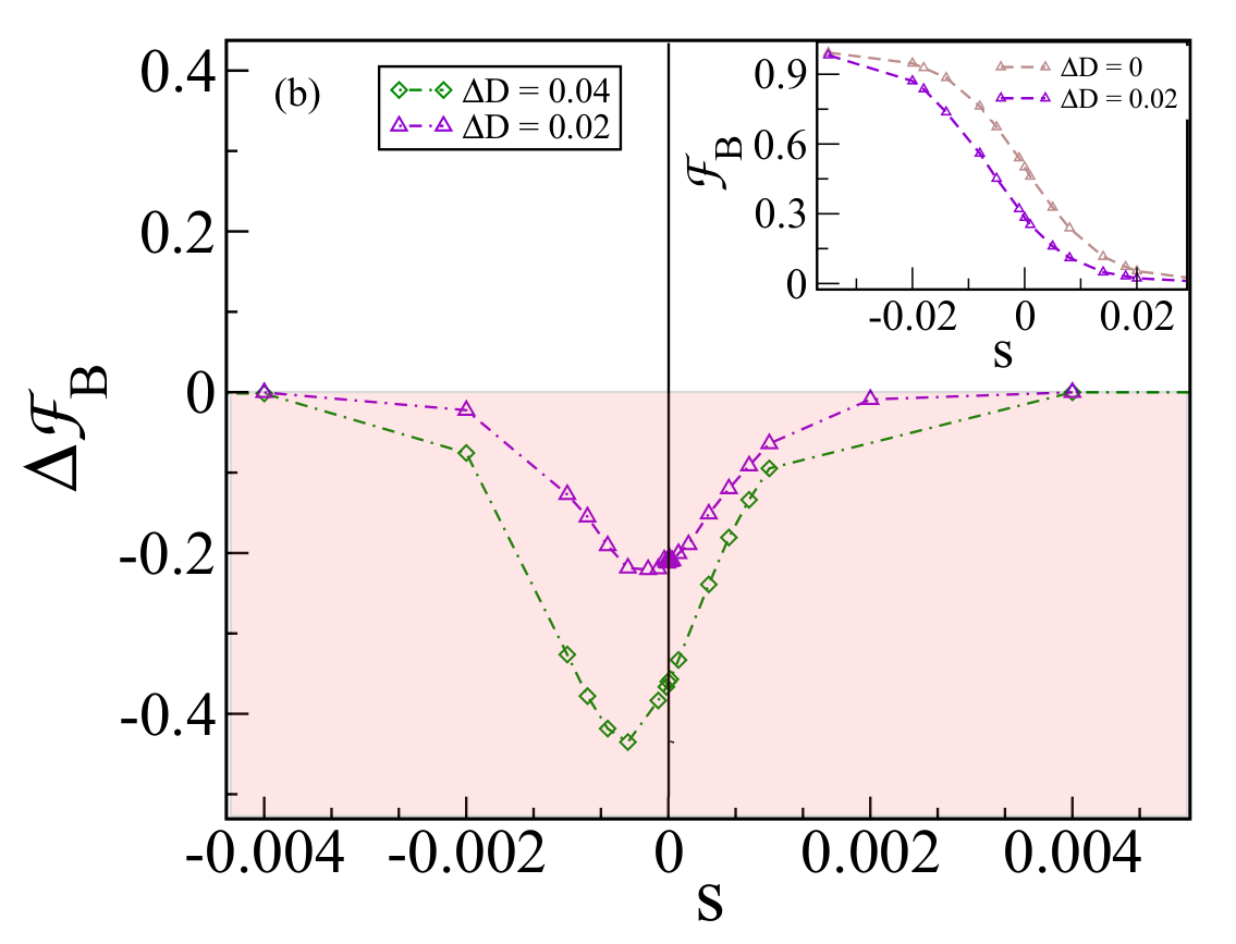
CLVMD: Reduction of $B$ diffusivity increases the residence time thus allowing more intra-species competition ($B+B\rightarrow B$) in time $\tau_{diff}$. The fall of the number of $B$’s makes $A$ fixation more likely on that site. For $s=0$, we already showed the faster species is favoured, implying $\Delta\mathcal{F}_{B}<0$. The fact that $\Delta\mathcal{F}_{B}(s,\Delta D)\to 0$ in Fig. 4(b) as $|s|$ increases follows from the same considerations as in the FVMD.

In this appendix we show the presence of a long lived quasi-steady state (QSS) in which $\langle N\rangle$ fluctuates around a constant value before eventual extinction. Our numerical simulations, even with small system size $L=8$ and density $\rho=2$, demonstrate that the fixation of one of the two species occurs well before extinction [see Fig. 6(top)]. For the large system sizes used in the main text, we are always in the QSS regime [see Fig. 6(bottom)].

References

- (1) J. M. Smith, Evolution and the Theory of Games (Cambridge Univ. Press, Cambridge, 1982).
- (2) J. Hofbauer and K. Sigmund, Evolutionary Games and Population Dynamics (Cambridge Univ. Press, Cambdrige, 1998).
- (3) M. A. Nowak, Evolutionary Dynamics (Belknap Press, Cambridge, Massachusetts, 2006).
- (4) V. Colizza and A. Vespignani, Phys. Rev. Lett. 99, 148701 (2007).
- (5) G. J. Baxter, R. A. Blythe, and A. J. McKane, Phys. Rev. Lett. 101, 258701 (2008).
- (6) M. Hamilton, Population Genetics (Wiley-Blackwell, New York, 2009).
- (7) S. A. Levin, Am. Nat. 108, 207 (1974).
- (8) J. D. Murray, Mathematical Biology: I. An Introduction, Third Edition (Springer-Verlag New York, 2002)
- (9) J. D. Murray, Mathematical Biology II: Spatial Models and Biomedical Applications, (Springer-Verlag New York, 2003)
- (10) S. H. Strogatz, Nonlinear Dynamics and Chaos: With Applications to Physics, Biology, Chemistry, and Engineering, Second Edition, Taylor and Francis (2014).
- (11) K. S. Korolev, M. Avlund, O. Hallatschek, and D. R. Nelson, Rev. Mod. Phys. 82, 1691 (2010).
- (12) D. Hartl and A. Clark, Principles of Population Genetics (Sinauer, Sunderland, 1989)
- (13) T. Reichenbach, M. Mobilia, and E. Frey, Nature Letters, 448, 1046 (2007).
- (14) S. Pigolotti and R. Benzi, Phys. Rev. Lett. 112, 188102 (2014).
- (15) S. Pigolotti and R. Benzi, J. Theor. Biol. 395, 204 (2016).
- (16) M. Deforet, C. Carmona-Fontaine, K.S. Korolev, and J.B. Xavier, The American Naturalist, 194, 291 (2019).
- (17) K. S. Korolev, Phys. Rev. Lett. 115, 208104 (2015).
- (18) D. Bhat and J. Piñero, and S. Redner, J. Stat. Mech. : Theor. and Exp. 2019, 063501 (2019).
- (19) S. Pigolotti, R. Benzi, P. Perlekar, M. H. Jensen, F. Toschi, and D. R Nelson, Theor. Pop. Biol. 84, 72 (2013).
- (20) C. R. Doering, C. Mueller, and P. Smereka, Physica A 325, 243 (2003).
- (21) T. Chotibut and D. R. Nelson, Phys. Rev. E 92, 022718 (2015).
- (22) N. Rana, P. Ghosh, and P. Perlekar, Phys. Rev. E 96, 052403 (2017).
- (23) P.A.P. Moran, Mathematical Proceedings of the Cambridge Philosophical Society, 54, 60 (1958).
- (24) J. Crow, and M. Kimura, An Introduction to Population Genetics Theory (Harper Row, New York, 1970)
- (25) P. Clifford and A. Sudbury, Biometrika, 60, 581 (1973).
- (26) R. A. Holley and T. M. Liggett, Ann. Probab. 3, 643 (1975).
- (27) A. Gabel, B. Meerson, and S. Redner, Phys. Rev. E, 87, 010101(R) (2013) discuss a similar quasi-steady state in a slightly different model of competition in the well-mixed regime.
- (28) M. Kimura, and G. Weiss, Genetics 49, 561 (1964).
- (29) M. Kimura, Ann. Rept. Nat. Inst. Genetics 3, 62 (1953).
- (30) S. Pigolotti, R. Benzi, P. Perlekar, M. H. Jensen, F. Toschi, and D. R Nelson, Theor. Pop. Biol. 84, 72 (2013).
- (31) C. R. Doering, C. Mueller, and P. Smereka, Physica A 325, 243 (2003).
- (32) A. Gabel, B. Meerson, and S. Redner, Phys. Rev. E 87, 010101 (2013).
- (33) H. Risken, Fokker-Planck Equation, Springer, Berlin, Heidelberg, (1984).
- (34) N.G. Van Kampen, Stochastic Processes in Physics and Chemistry, edition (2007).
- (35) R.A. Fisher, Ann. Eugenics 7, 353 (1937).
- (36) A. Kolmogorov, I. Petrovsky, N. Piscounov, Moscow Univ. Bull. Math. 1 (1937) 1.
- (37) Daniel T. Gillespie, Annu. Rev. Phys. Chem. 58 35, (2007).