Probabilistic Detection and Estimation of Conic Sections from Noisy Data
Abstract
Inferring unknown conic sections on the basis of noisy data is a challenging problem with applications in computer vision. A major limitation of the currently available methods for conic sections is that estimation methods rely on the underlying shape of the conics (being known to be ellipse, parabola or hyperbola). A general purpose Bayesian hierarchical model is proposed for conic sections and corresponding estimation method based on noisy data is shown to work even when the specific nature of the conic section is unknown. The model, thus, provides probabilistic detection of the underlying conic section and inference about the associated parameters of the conic section. Through extensive simulation studies where the true conics may not be known, the methodology is demonstrated to have practical and methodological advantages relative to many existing techniques. In addition, the proposed method provides probabilistic measures of uncertainty of the estimated parameters. Furthermore, we observe high fidelity to the true conics even in challenging situations, such as data arising from partial conics in arbitrarily rotated and non-standard form, and where a visual inspection is unable to correctly identify the type of conic section underlying the data.
Keywords: Bayesian hierarchical model; Bernstein basis polynomials; focus-directrix approach; Markov Chain Monte Carlo; Metropolis-Hastings algorithm; partial conics
1 Introduction
In many practical scenarios in computer vision, camera calibration, and image recognition, among many others (Ayache, 1991; Forstner, 1987; Beck and Arnold, 1977; Ballard and Brown, 1982; Szpak et al., 2012, e.g.,), it is of interest to estimate curves or surfaces based on a set of noisy data. Specifically, consider a random sample of paired observations which are assumed to arise from a joint distribution of generic pair . It is known that and , where denotes bivariate independent noise or error, and that the support of the unobserved pair lies on a conic section.
For instance, in Figure 1, we illustrate three cases where the samples are drawn from three popular conic sections, parabola, hyperbola and ellipse. Without first hand knowledge about the specific nature of the underlying support of the random pair , it is visually difficult to guess the support of the pair of random variables, even when we have first hand knowledge that the support belongs to a conic section. Moreover, the usual least squares based methods for a statistical model, i.e., , where denotes the regression function, are not readily applicable for these type of data and would often lead to erroneous inferences. This is primarily because a given value of does not correspond to a unique value of the underlying variable . This motivates us to develop models and associated methodologies that would not only enable us to estimate the underlying parameters of a given conic section (e.g., being ellipse, parabola or hyperbola), but also provide probabilistic detection of the hidden type of conic section.
In many applications, there are practical consequences of misclassifying the type of conics, e.g. incorrectly classifying a parabola as a hyperbola. A classic example is estimating the orbit of a smaller body (e.g. a planet or exoplanet) around a larger body (e.g. a star) which takes the shape of an ellipse, with the larger body being at one of the two focal points of the ellipse. This definitely has become of great significance in modern astronomy when discovering new exoplanets. The website https://exoplanets.nasa.gov/ has many recent applications. Another application is that of the correct identification and estimation of parabolas and hyperbolas in the field of optics. For example, car headlights are often in a parabolic shape because this causes a highly focused beam of light in front of the car and real-time estimation of its focus is of great importance in modern automated cars. For many other interesting modern applications, refer to Yaqi et al., 2019.
For a quick glimpse of our proposed method, in Figure 1, we present the fitted conic section using the solid blue lines overlayed on a set of simulated data points generated from partial conics. The variance of the added bivariate Gaussian noise was the same in each dataset. (However, the noise appears to be less for the parabola and hyperbola because they are not compact, and their data have much greater ranges than the ellipse.) The data were analyzed assuming that we were unaware of the type of true conic section. The estimation uncertainty is indicated by the gray curves, which represent samples drawn from conservative 95% posterior credible intervals for the conics, and correspond to multiplicity-adjusted, Bonferroni-type intervals for the univariate conics hyperparameters. The posterior probabilities of the detected types of conic sections for each of the three data sets are displayed in Table 1. We find that in all three examples, the probability of detecting the true type of hidden conic section is nearly perfect. This is particularly interesting given that data generated from a true parabola could be easily misjudged to have come from a true ellipse, and vice versa.
| Posterior classification probabilities | |||
|---|---|---|---|
| Ellipse | Parabola | Hyperbola | |
| Parabola #38 | 0.005 (0.005) | 0.995 (0.005) | 0.000 |
| Hyperbola #9 | 0.000 | 0.000 | 1.000 |
| Ellipse #90 | 1.000 | 0.000 | 0.000 |
In the vast literature on conics and in several engineering applications over the past several decades, many novel and computationally efficient methods have emerged that provide the ‘best’ fit of the underlying conic section when it is known that underlying conic section is an ellipse (or circle), parabola or hyperbola (Prasad et al., 2013; Ahn et al., 2001; Zhang, 1997; Szpak et al., 2012, e.g.,). However, to the best of our efforts, we were unable to find any methodologies that provide probabilistic inference about the underlying nature of the conic section based on noisy observations.
In essence, we provide an answer to the following motivating question: Given a set of noisy observations, where , and the fact that belongs to a conic section, can we estimate the probability that the support of is an ellipse, a parabola or a hyperbola? Answers to such a question are of immense practical value in computer vision and image detection, as we will show that even when the observations arise from only a portion of the (unknown) underlying conic section, our proposed method is able to not only estimate the parameters of the conic section but also provide an estimate of the probability of the detected conic type.
| . |
In order to define our models and associated methodologies, we first present some basic notions of conic sections, which although easily found in any elementary mathematics textbook dealing with conic sections, helps us to fix the notation to be used throughout the rest of this paper.
A conic section is produced when a plane intersects with a right circular conical surface. The three types of conics that results are known as ellipses (which includes circles), parabolas, and hyperbolas. There are many different formulations for a conic section based on Cartesian coordinates (algebraic definition) or polar coordinates (based on focus-directrix definition). We start with the latter as we find that formulation most useful for our purposes.
1.1 Focus-directrix definition of conics using polar coordinates
Among the different equivalent representations of conics, one of the most useful is the focus-directrix approach. It involves a fixed point called the focus, a line not containing called the directrix, and a nonnegative number called the eccentricity (not to be confused with the Euler number ). A conic section is defined as the locus of all points for which the ratio of their distance to to their distance to , is equal to . We obtain an ellipse when , a parabola when , and a hyperbola when . A circle is an ellipse with . See Akopyan and Zaslavsky, 2007 and Samuel, 1988 for a comprehensive review of the basic concepts of conics. See Figure 2 for a graphical illustration.
Denote by the line containing the axis of symmetry in the case of a hyperbola or parabola, and containing the major axis in the case of an ellipse. Line contains the focus in all three types of conic sections. The rotation angle of the conic is defined as the counterclockwise angle, , from the positive X-axis to the line . Given a conic point, , denote by the line segment connecting this point to the focus. Then the point satisfies the equation
| (1) |
where is the length of the segment , is the counterclockwise angle from the line to the segment , and is a positive constant known as the semi-latus rectum. Figure 2 graphically illustrates these concepts. Due to the radial symmetry of a circle, the line is not uniquely defined, and can be arbitrarily taken to be parallel to the positive X-axis.
The angles belong to the interval , where
| (2) |
Consequently, for ellipses and parabolas, angle is unrestricted and belongs to the interval . For hyperbolas, angle belongs to the interval . The vector of hyperparameters uniquely determining the conic section is . Distance in equation (1) is a function of parameter and angle . Transforming from polar to Cartesian coordinates, and explicitly specifying the dependence on the model parameters, we obtain the following equations for any conic point, :
| (3) | ||||
1.2 Quadratic equation definition using Cartesian coordinates
An equivalent and more popular formula for a conic point is
| (4) |
where , and are not simultaneously zero. Without loss of generality, and for identifiability of these parameters, we may assume that ; other restrictions are also available in the literature, e.g., see (Zhang, 1997). We denote the vector as representing the parameters of the conic section. Notice that due to the restriction, lies in a 5-dimensional space. It can be shown that there is a one-to-one map between the parameter of the focus-directrix formulation and parameter of the algebraic formulation. Defining the constant , and the matrix determinants
the additional assumptions that , , and guarantee that equation (4) represents an ellipse rather than a hyperbola or parabola. Let be the parameter space corresponding to these additional constraints on vector . It follows that there exists a one-to-one mapping between elements of the parameter space and the parameter space defined in Section 1.1 (Silverman, 2012, e.g., see). Thus, for statistical estimation we can work with either parametrization. Finally, we present the formulation of conics in the most popular standard form by centering and rotation.
1.3 Conics in standard form
We define the center of a conic as follows. For an ellipse, it is the midpoint of the segment joining the two foci. For a parabola, the center is the point at which the axis of symmetry intersects the parabola. For a hyperbola, it is midway between the foci of the two branches. A conic in standard form has its center at the origin and rotational angle .
Identifiability of angle in standard form
We assume that in standard form, parabolas are left-opening, ellipses have the horizontal axis as their major axes, and we consider only the left branch of hyperbolas. Right-opening hyperbolas are regarded as rotated versions of left-opening hyperbolas with angle . These assumptions ensures that rotational parameter is identifiable when estimating this parameter based on noisy data. The equations for standard conics are then given for :
- Ellipses:
-
A standard ellipse has the equation .
- Hyperbolas:
-
A (left-opening) standard hyperbola has the equation .
- Parabola:
-
A left-opening standard parabola has the equation .
Notice that the focus is different from the conic center and has a different expression for each kind of conic in standard form. Whereas the center coincides with the origin, the expression for depends on the constant in the case of parabolas, and on the constants and in the case of ellipses and hyperbolas.
Converting a conic equation to standard form
Let be a point lying on an arbitrary (non-standard) conic whose center is . We make the transformation:
| (5) |
Then the conic equation expressed in terms of is in standard form.
1.4 Estimation of conic parameters with known type
There is vast literature on numerical methods for the estimation of parameters of a given conic section when it is known that the (noisy) data arise from one of the three basic types of conic sections. For instance, Zhang, 1997 presents a very comprehensive review of several commonly used techniques, including linear least-squares (pseudo-inverse and eigen analysis), orthogonal least-squares, gradient-weighted least-squares, and bias-corrected renormalization. Prasad et al., 2013 proposed a method specifically designed for fitting ellipses using the geometric distances of the ellipse from the data points. Given a specific type of conics, Ahn et al., 2001 provide various estimation methods for different types of conics sections using least-squares with respect to various predefined measures.
However, none of these above mentioned methodologies are able to provide probabilistic inference about the underlying hidden type of a conic section. Moreover, as the majority of these earlier methodologies are based on some form of optimization (that minimizes a chosen distance between the observed points and the known type of conic section), uncertainty estimates for the conic parameters are not readily available. Thus, full statistical inference including standard errors of estimates is often missing in some of these earlier works. Bootstrap methods could perhaps be used to obtain standard errors of these earlier estimates, but that would require establishing asymptotic theory of the underlying data measured with errors when the support of the true data is a given conic section.
We instead adopt a model-based, fully Bayesian hierarchical approach using the focus-directrix formulation, which facilitates the complete probabilistic inference of not only the parameters for a given type of conic section, but also provides the posterior probability of classification for the conic section type. The proposed estimation technique relies on a Bayesian computational approach and the focus-directrix representation to model the data and obtain the entire posterior distribution of the conics parameters. It has several practical and methodological advantages that make it an important addition to the aggregation of existing inferential techniques for conics.
The advantages the proposed method include the ability to: (i) provide a coherent, integrated framework for flexibly fitting different conic sections (hyperbola, parabola, ellipse, and circle), (ii) make accurate inferences on the unknown type of conic section underlying the data, (iii) compute uncertainty estimates for all the model parameters, and (iv) achieve high fidelity to true conics even in challenging inferential situations, such as noisy data arising from partial conics in arbitrarily rotated and non-standard form. As the simulation studies in Section 3 demonstrate, the technique is impressively accurate even in noisy, partial datasets like Figure 1, where a visual inspection is unable to correctly call the hidden type of conic section underlying the data.
2 A Bayesian Inferential Framework for Conics
2.1 The hierarchical model
Bayesian models typically consist of a sampling (conditional) distribution of the data given the possibly vector-valued model parameter. This contributes towards the calculation of the likelihood function of the parameter. Additionally, the model requires specification of the marginal probability distribution for the parameter, which is commonly known as the prior distribution. Then, using the Bayes’ Theorem, we obtain the conditional distribution of the parameter given the observed data, commonly known as the posterior distribution. For a majority of the Bayesian models, it is impossible to obtain the analytical form of the posterior distribution. Markov Chain Monte Carlo (MCMC) methods are then utilized to draw approximate samples from the posterior distribution (Gelman et al., 2014, e.g.,).
Likelihood function
The noisy observations are modeled as arising from a set of latent conic points contaminated by independent Gaussian errors. In other words, referring back to the focus-directrix approach of Section 1.1, the observations can be represented as:
| (6) |
for and with an unknown denoting the measurement error variance. It is possible to relax the assumptions on the error by extending it to a bivariate distribution that allows for correlated errors, but in order to keep the exposition simple, we work with the i.i.d. case. However, in real applications, one may wish to check the distributional assumption of the errors by an appropriate suite of goodness-of-fit tests (Huber-Carol et al., 2002). The Cartesian coordinates of the latent conic point is given in equation (3). Let be the set of (unobserved) angular parameters and parameter vector be the full set of hyperparameters. Conditional on the latent angular variables, the model implies the following (conditional) joint density function for the data given the angular variables:
| (7) |
where the symbol represents the probability density function of a normal distribution with mean and variance evaluated at the point . Later, we provide details on how we model the latent angular parameters . Next, we specify the prior probability distributions of the parameters of the conic sections.
Eccentricity
This parameter is key because it identifies the type of conic section (ellipse, parabola, or hyperbola) underlying the data. In the absence of any prior information about the relative abundances of the three conics, it is reasonable to assume that the three conics types are equally likely. That is, . Clearly, we can not use any probability distribution on that is dominated by a Lebesgue measure as it will not allow for a positive probability for circles and parabolas. Thus, we need to use a slightly non-standard prior for that allows positive probabilities for the events and , facilitating posterior inferences about this important parameter.
Let be a continuous CDF with support and median greater than 1. That is, , , and . We specify the prior for eccentricity parameter as follows:
| (8) |
with the last branch corresponding to the condition , i.e., non-circular ellipses as well as hyperbolas. Prior (8) implies that , so that ellipses, parabolas, and hyperbolas are apriori equally likely, yielding a mixture prior on the different types of conics.
We allow the user to choose suitable prior distributions within the above set up, and later through simulation studies, demonstrate that the posterior inferences are relatively insensitive to such prior choices. Specifically, if distribution is such that (e.g., exponential distribution with mean 1.557), we obtain the following prior for the eccentricity parameter:
| (9) |
Posterior inferences are made about the probability that the conic section underlying the noisy data is a particular type, e.g., parabola. The posterior probabilities in Table 1 were computed in this manner. If interest focuses on the Bayes factor for a conic type, this can be easily evaluated from the posterior probabilities. For example, consider the data generated by Parabola #38 in Table 1. The estimated posterior probability of the event is , corresponding to a posterior odds of . The prior odds is . The Bayes factor in favor of the hypothesis that the underlying conic is a parabola, versus the alternative hypothesis that it is not a parabola, is therefore the ratio of the posterior odds to the prior odds, i.e., . This is overwhelming evidence in favor of parabolas. For Hyperbola #9 and Ellipse #90, the Bayes factors in favor of the true conics are computationally infinite.
Angular parameters
Let be a version of angle standardized to the unit interval. Specifically, let
| (10) |
Clearly, prior to being given the noisy data, we do not have any strong information about the distributional shape of the angular variables, and so it is reasonable to model these latent variables using a flexible class of probability distributions that would not impact the posterior inference, and would additionally allow arbitrary shapes for the density functions (e.g., symmetric, skewed, bimodal).
We adopt a mixture of (a known sequence of) Beta densities which has been shown to approximate any continuous density supported on the unit interval (Vitale, 1975; Babu et al., 2002; Ghosal, 2001). Given any continuous density supported on , it can be shown that converges uniformly to as if we choose for and define . Motivated by this uniform convergence result, for a prespecified positive integer that is typically chosen to be large, we model the standardized angles as being apriori exchangeable and having a mixture of beta distributions:
| (11) |
Here, denotes a Dirichlet distribution on categories with the concentration parameters all equal to . Prespecifying gives satisfactory results in most applications.
In addition to simplicity of implementation, this framework has important advantages. Being a linear combination of Bernstein basis polynomials of degree , the prior density is able to closely approximate any true continuous density of the angular parameters, provided is large enough (Natanson, 1964, e.g.). In fairly general situations, applying an asymptotic result of Babu et al., 2002, Turnbull and Ghosh, 2014 recommend setting the degree .
Hyperparameters
The eccentricity , semi-latus rectum , and center coordinates and are all assigned independent Gaussian prior distributions, restricted to the positive real line for the parameters that are positive. The rotational angle is assigned a uniform prior on the interval . Variance is given an inverse gamma prior.
2.2 Posterior inferences
Initial estimates for the model parameters are computed as described in Section 2.2.1. With these estimates as the starting values, the model parameters are iteratively updated using the MCMC steps outlined in Section 2.2.2. Subsequently, the post–burn-in MCMC sample is used to make posterior inferences.
2.2.1 Initialization procedure for MCMC algorithm
We first present a basic result:
Lemma 2.1
Let be a point on the conic with center . Transform to obtain point as follows:
| (12) |
This transformation rotates the conic point clockwise around the origin by an angle of . Similarly, center is premultiplied by the square matrix appearing in equation (12) to obtain the rotated center, .
- 1.
Suppose the conic section is either an ellipse () or hyperbola (). Then
(13) where , , , and .
- 2.
Suppose the conic section is a parabola. Then
(14) where , , and .
The proof of the Lemma uses equation (5), which converts the conic equation to standard form, and involves making use of standard well-known results (e.g. Fanchi, 2006, pp. 44–45) and some tedious algebra that we have omitted for brevity.
The starting parameters are computed as follows:
- 1.
Using the quadratic equation representation of conics (see Section 1.2), we apply the least-squares fitting approach of (Zhang, 1997, Sec. 4.2) to compute a preliminary estimate, , of the conic parameters.
- 2.
It can be shown that the true rotational angle, , satisfies . Let , so that . Possible estimates for the true unknown , which may belong to , are then contained in the set
with the symbol denoting a wrapped angle belonging to the interval , e.g., .
- 3.
For each of the four candidate estimates, :
- (a)
Use angle to rotate the data point clockwise around the origin and thereby obtain the point . Similar to equation (12), this is done by premultiplying vector by the square matrix determined by the angle .
- (b)
Assuming that the conic is an ellipse:
- i.
Based on expression (13), we find an estimate that minimizes the quantity . This is equivalent to computing the least squares estimate of in the model , where the independent errors have zero means and equal variances. Using these estimates, we apply Part (1) of Lemma 2.1 to estimate the ellipse parameters , which is in one-to-one correspondence with the estimated parameters of the focus-directrix approach, denoted by .
- ii.
Applying expression (3) of the present paper, we express the nearest conic point to the datum as for some optimal angle . In other words,
where expression (2) of the paper gives the support for an ellipse. Consequently, the initial estimate can be found by a univariate optimizer over the interval . This procedure is repeated for the data points to get an initial estimate for the vector of angular parameters.
- iii.
Expression (7) is maximized over to obtain the likelihood function for the best-fitting ellipse corresponding to rotational angle . Let the likelihood function for the best-fitting ellipse be denoted by .
- i.
- (c)
Assuming that the conic is a hyperbola, we perform a similar initialization procedure to Part 3b. The only difference is with Part 3(b)ii in which, applying expression (3) of the main paper, the support of the univariate optimizer for the angles of a hyperbola is where is the eccentricity parameter estimated as part of parameter vector for the focus-directrix approach. We thereby obtain the likelihood function, , for the best-fitting hyperbola corresponding to the rotational angle .
- (d)
Assuming that the conic is a parabola, we perform a similar initialization procedure to Part 3b. The only difference is in Part 3(b)i, in which we instead apply expression (14) in Part (2) of Lemma 2.1 to obtain the estimated parameter for the parabola. In this manner, we obtain the likelihood function, , for the best-fitting parabola corresponding to the rotational angle .
- (e)
Compute the overall maximized likelihood over the conic types for the rotational angle :
- (a)
- 4.
Set the estimated rotational angle to the candidate angle with the greatest overall maximized likelihood. That is, where .
- 5.
2.2.2 MCMC updates
With the estimates from the previous section as the initial values, the model parameters are iteratively updated using the following MCMC algorithm.
Eccentricity parameter
For conditionally updating the parameter , it can be shown that the upper bound for equals if exceeds , and equals otherwise (Silverman, 2012, e.g.,). Ideally, we would like to compute the posterior probabilities of the three branches of the prior (9). However, the third branch involves a marginal likelihood calculation for a non-conjugate part of the model. We therefore apply the Laplace approximation to obtain an approximate, conjugate normal model with restricted support, for which the marginal likelihood is available in computationally closed form. This approximate model is used to propose a new parameter value that is either accepted or rejected with a Metropolis-Hastings (MH) probability to obtain draws from the true conditional posterior of the parameter .
Inferred type of conic section
We define a categorical variable identifying the type of conic section from the eccentricity parameter:
| (15) |
The detected type of conic section is the mode of the post–burn-in MCMC samples of this categorical variable. Empirical average estimates of the posterior probabilities of the four categories, along with their uncertainty estimates, are also readily available from the MCMC sample. The results displayed in Table 1 were computed in this manner.
Remaining model parameters
The hyperparameters , , and can be updated by Gibbs sampling because of the model’s conditional conjugacy in these parameters. Parameters and are conditionally updated by random walk MH moves. For updating these parameters, the normal proposal distribution’s variance is set equal to a constant times the inverse Fisher information matrix, with the constant chosen to achieve an empirical acceptance rate of 25% to 40% for the MH proposals. For obtaining fast-mixing MCMC chains, this is the recommended range of acceptance rates in overdispersed random walk MH algorithms (Roberts et al., 1997). Due to relation (2), the normal proposals for the angle parameters are restricted to the interval for ellipses and parabolas, and to the interval for hyperbolas. Finally, the relative weights of the beta prior distributions in expression (11) are updated using the current values of the angles .
2.2.3 Posterior Estimation and credible intervals for the true conic
Recall that, in the focus-directrix approach, hyperparameter uniquely determines the conic from which the noisy data have been generated. Using the post–burn-in MCMC sample, the empirical average of the sampled values of vector provides a point estimate for the true conic section. The estimated curves in Figure 1, displayed by the blue bold lines, were computed in this manner.
Uncertainty estimates for the true conic are also available. Suppose we are interested in a % posterior credible region (CR) for the true conic, for some . Using the MCMC sample, we compute % marginal posterior credible intervals (CIs) for each component of hyperparameter . Then the Cartesian product of those five CIs is a conservative % posterior CR for the true conic. In Figure 1, the gray lines represent conic samples generated from conservative 95% CRs of this type. We find from Figure 1 that these curves are good fits for the data, even in the case of the ellipse, where the sampled conics provide appropriate coverage for the noisy data points.
Since hyperparameter is not high-dimensional, we do not expect the Bonferroni-type adjustments for the CIs to be too conservative in general. However, this is certainly possible in some studies, especially when the components of are highly correlated in the posterior. In these situations, to overcome the issue of marginalizing over the angular parameters and variance , we recommend the following computational strategy to avoid an overly conservative CR. The MCMC sample is post-processed to estimate the posterior mean and variance matrix of . A sample of values is generated from the 5-variate normal distribution having this mean and variance, which represents a large-sample approximation to the marginal posterior density of . Evaluating the approximately normal densities for these sampled , and retaining only those belonging to the top 95th percentile of densities, gives an approximate 95% highest posterior density CR for the true conic.
3 Numerical illustrations using simulated data scenarios
The artificial datasets in Section 3.1 were generated using the simulation strategy of Zhang, 1997. We investigate the accuracy with which we are able to infer the ellipse parameters from noisy data, including estimation of the rotational angle . Artificial data were generated from partial as well as complete true ellipses. In Section 3.1, we assume that the type of conic section, e.g. ellipse, is known, and focus on estimating the ellipse parameters. We relax this assumption in the next set of simulations in Section 3.2, generating data from partial ellipses, parabolas, and hyperbolas having randomly generated rotational angles and other model parameters.
3.1 Simulation Study 1
We investigated the ability of the Bayesian procedure to detect standard-form ellipses from noisy data. Similar to the strategy of Section 3.2 and Section 10.1 of Zhang, 1997, we assumed that the true conic is an ellipse with the following parameters: the major axis equals units, the minor axis equals units, the center is at , and the rotation angle is 0 degrees.
We generated data points with the standardized angular parameters, defined in equation (10), generated as for . From these values, the angular parameters were computed. A rotational angle of was assumed. A bivariate error with independent Gaussian components having mean 0 and standard deviation was added to each ellipse point to obtain the corresponding data point.
The procedure was repeated to obtain 100 simulated datasets each of size . For a typical dataset, the top panel of Figure 3 displays the data points using black dots and the true ellipse using the red solid line. Since the density for the angular parameters has the mode at 0 radians, the data points are more highly concentrated near the left corner of the ellipse upon applying the rotation of .
| Simulation 1 | |||
|---|---|---|---|
| Long axis | Short axis | Center | |
| True values | () | () | |
| Biases | |||
| Pseudo inverse | -0.718 | 0.192 | (249.733, 250.019) |
| Orthogonal distance | -0.194 | 0.016 | (249.778, 250.024) |
| Bayes | -0.420 | -0.024 | (249.780, 250.034) |
| Standard errors | |||
| Pseudo inverse | 0.142 | 0.050 | (0.062, 0.024) |
| Orthogonal distance | 0.140 | 0.048 | (0.061, 0.023) |
| Bayes | 0.136 | 0.046 | (0.059, 0.022) |
Each dataset was analyzed using the methods pseudo inverse (Zhang, 1997, Sec. 4.1), orthogonal distance fitting, and the Bayesian approach of Section 2 conditional on the conic section being an ellipse. The first two methods were also investigated in Section 10.1 of Zhang, 1997. For analyzing the angular parameters in the Bayesian approach, following the recommendation of Turnbull and Ghosh, 2014, we set the degree of the Bernstein polynomial, .
The average bias in the parameter estimates and Monte Carlo (MC) standard errors for the 100 datasets are presented in Table 2. The root mean square errors (RMSEs) are then readily available as the sum of the corresponding squared biases and squared standard errors. We find that all three methods provide similar estimates that coincide with the truth within the margin of error. Averaging over the 100 datasets, the estimated ellipse by the Bayesian hierarchical approach is shown using the blue dashed line in the top panel of Figure 3.
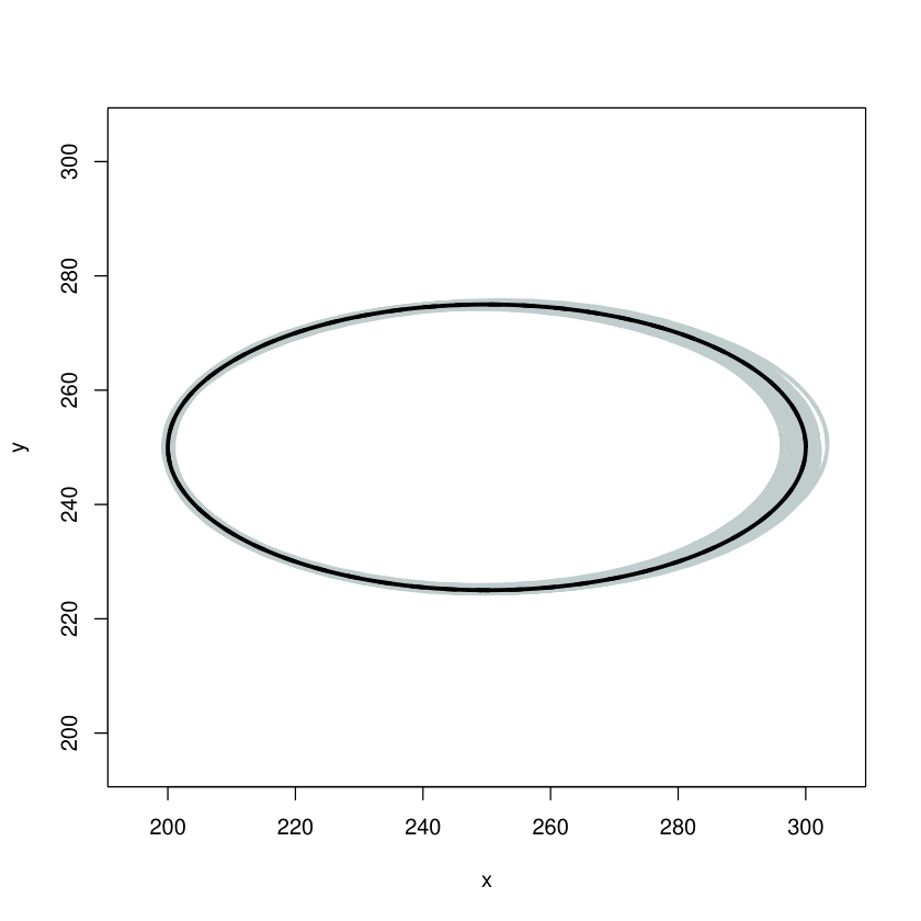
The bottom panel of Figure 3 displays the true ellipse (black) and the 100 estimated ellipses (gray) by the Bayesian method. We find that the contours of the estimated ellipses are highly concentrated around the true ellipse; a little more so near the left edge of the ellipse, where more data are available.
3.2 Simulation Study 2
We investigated the ability of the Bayesian procedure to detect the type of conic section from noisy data generated by conics in non-standard form, i.e., hyperbolas, ellipses, and parabolas with unknown focuses and arbitrarily rotated axes of symmetry. Furthermore, to increase the difficulty of making calls from a visual inspection, all the data were generated from partial conics, such as half-ellipses that may be incorrectly detected as hyperbolas or parabolas. Additional variability was introduced into the simulation by randomly generating the true conics parameters for each artificial dataset.
Specifically, we generated 300 artificial datasets with data points each. An equal number of datasets was allocated to true ellipses, parabolas, and hyperbolas. For each dataset, we performed the following steps to randomly generate the conic section parameters and the associated noisy data points:
- 1.
Referring back to the standard conics equations of Section 1.3, the true parameters and were generated from normal distributions with means 50 and 25 respectively, and with variances 4. For parabolas, only parameter was generated.
- 2.
Rotational angle was uniformly generated from the interval .
- 3.
The conic center was fixed at .
- 4.
The angular parameters for the conic points, defined in equation (2), were generated as follows:
- (a)
For ellipses, only one half of the curve was used to generate the data. Specifically, we generated .
- (b)
For hyperbolas, we first computed the eccentricity and uniformly generated the parameters ’s over the range specified in equation (2).
- (c)
For parabolas, we generated the angular parameters as .
- (a)
- 5.
Depending on the type of conic section, the semi-latus rectum and eccentricity were computed using well-known formulas that involve parameters , and conic center .
- 6.
- 7.
To both components of the conic points, add independent, zero-mean Gaussian errors with standard deviation to obtain the data, for .
For example, a randomly chosen ellipse, hyperbola, and parabola are shown in Figure 1. Observe that, being randomly generated, the center, rotational angle, and other parameters are all different in the three conics. Gaussian random noise with was added to generate each data point in all three conics. However, parabolas and hyperbolas have unbounded one-dimensional “surfaces” or line integrals, and their data have much greater ranges than those of ellipses, as seen in Figure 1.
Assuming all conic parameters to be unknown, the MCMC procedure based on the categorical variable defined in equation (15) was used to identify the type of conic in each dataset. The type of conic section was correctly detected in 276 (i.e., 92%) of the datasets. Table 3 provides more detail about the estimated posterior probabilities of detection and misclassification for each type of conic, revealing that ellipses and hyperbolas were rarely or never misclassified. Parabolas were misclassified 21.4% of the time. A possible explanation is that parabolas are represented by the singleton value of , with values to the left representing ellipses and values to the right representing hyperbolas. Averaging over the 300 datasets, the root mean squared error for the eccentricity parameter was 0.051.
For analyzing these data, the proposed technique took, on average, 0.01621 seconds per MCMC iteration on a PC laptop with Intel Core i7 CPU and 8 GB RAM. Despite the high dimensionality of the parameter space, a few thousand MCMC iterations were found to be more than sufficient for accurate posterior inferences due to the fast-mixing MCMC chain.
The proposed method, like Bayesian hierarchical approaches in general, is computationally intensive when compared with several frequentist approaches for conic sections. However, the benefits far outweigh the computational costs, since the Bayesian method not only provides accurate estimates, along with uncertainty estimates, for all parameters of interest, but also detects the underlying types of conic section.
| Detected | |||
|---|---|---|---|
| True | Ellipse | Parabola | Hyperbola |
| Ellipse | 1.000 (0.000) | 0.000 (0.000) | 0.000 (0.000) |
| Parabola | 0.131 (0.034) | 0.786 (0.041) | 0.083 (0.027) |
| Hyperbola | 0.000 (0.000) | 0.030 (0.017) | 0.970 (0.017) |
4 Discussion
We have proposed a coherent and flexible Bayesian hierarchical model for fitting all possible conic sections to noisy observations. The methodology is able to accurately compute estimates and uncertainty estimates for all the conic parameters. The success of the technique was demonstrated via simulation studies in which the data were generated from partial as well as complete true ellipses. In the simulation study, we explored the probabilistic detection of the underlying conics by generating the data from several partial conics, such as half-ellipses that may be incorrectly detected as hyperbolas or parabolas. For each artificial dataset in this study, additional variability was introduced by randomly generating the true conics parameters including the rotational angle and conic type. The simulation results indicate that our proposed method has low misclassification rates irrespective of the underlying conic type.
Through further simulation studies, we have found that when the data are generated from only a part of the conic section, our method may produced biased estimates for the conic parameters, even though it is able to correctly identify the type of conic section. This is also true for the estimates produced by other competing methods in the literature (when they are supplied addition information about true underlying conic type). Further details of the comparisons can be found in Section 1 of the Appendix.
There is empirical evidence that the proposed technique may lead to large sample consistent estimates. That is, as the number of data points grows, the inference procedure is able to detect the conic section parameters with greater accuracy (e.g., see Kukush et al., 2004 for consistency using least squares-type methods). In this paper, we have not pursued theoretical properties such as the posterior consistency of the estimates and their rates Ghosal and van der Vaart, 2017. Extensions of our methodology to other curved planes and surfaces are also of interest. This would perhaps require a more substantial development than those presented in this paper, and hence remains a part of future developments in this topic.
SUPPLEMENTARY MATERIALS
- BayesConics.zip:
-
R code for reproducing the Simulation Study 2 results of Section 3.2. The code performs three functions: (a) generates artificial datasets, (b) analyzes the generated data using the proposed Bayesian methodology to detect the underlying conic type, and (c) provides a summary of the detection accuracy, presented in Table 3. The README file in the zip folder contains instructions for use.
References
- Ahn et al., (2001) Ahn, Sung Joon, Rauh, Wolfgang, and Warnecke, Hans-Jürgen (2001), “Least-squares orthogonal distances fitting of circle, sphere, ellipse, hyperbola, and parabola,” Pattern Recognition, 34, 2283–2303.
- Akopyan and Zaslavsky, (2007) Akopyan, A.V. and Zaslavsky, A.A. (2007), Geometry of Conics, American Mathematical Society.
- Ayache, (1991) Ayache, N. (1991), Artificial Vision for Mobile Robots: Stereo Vision and Multisensory Perception, MIT Press, Cambridge, MA.
- Babu et al., (2002) Babu, G., Canty, A., and Chaubey, Y. (2002), “Application of Bernstein polynomials for smooth estimation of a distribution and density function,” Journal of Statistical Planning and Inference, 105, 377–392.
- Ballard and Brown, (1982) Ballard, D.H. and Brown, C.M. (1982), Computer Vision, Prentice-Hall, Englewood Cliffs, NJ.
- Beck and Arnold, (1977) Beck, J.V. and Arnold, K.J. (1977), Parameter Estimation in Engineering and Science, Wiley series in probability and mathematical statistics, Wiley, New York.
- Fanchi, (2006) Fanchi, John R. (2006), Math refresher for scientists and engineers, John Wiley and Sons.
- Forstner, (1987) Forstner, W. (1987), “Reliability analysis of parameter estimation in linear models with application to mensuration problems in computer vision,” Comput. Vision, Graphics and Image Processing, 40, 273–310.
- Gelman et al., (2014) Gelman, Andrew, Carlin, John, Stern, Hal, Dunson, David, Vehtari, Aki, and Rubin, Donald (2014), Bayesian Data Analysis, Third Edition, Chapman & Hall/CRC Texts in Statistical Science.
- Ghosal, (2001) Ghosal, S. (2001), “Convergence rates for density estimation with bernstein polynomials,” The Annals of Statistics, 29, 1264–1280.
- Ghosal and van der Vaart, (2017) Ghosal, Subhashis and van der Vaart, Aad (2017), Fundamentals of Nonparametric Bayesian Inference, Cambridge Series in Statistical and Probabilistic Mathematics.
- Huber-Carol et al., (2002) Huber-Carol, C., Balakrishnan, N., Nikulin, M. S., and Mesbah, M. (eds.) (2002), Goodness-of-Fit Tests and Model Validity, Springer.
- Kukush et al., (2004) Kukush, Alexander, Markovsky, Ivan, and Huffel, Sabine Van (2004), “Consistent estimation in an implicit quadratic measurement error model,” Computational Statistics & Data Analysis, 47, 123–147.
- Natanson, (1964) Natanson, I.P. (1964), Constructive function theory. Volume I: Uniform approximation, New York: Frederick Ungar.
- Prasad et al., (2013) Prasad, Dilip K., Leung, Maylor K.H., and Quek, Chai (2013), “ElliFit: An unconstrained, non-iterative, least squares based geometric Ellipse Fitting method,” Pattern Recognition, 46, 1449–1465.
- Roberts et al., (1997) Roberts, G. O., Gelman, A., and Gilks, W. R. (1997), “Weak Convergence and Optimal Scaling of Random Walk Metropolis Algorithms,” Annals of Applied Probability, 7, 110––120.
- Samuel, (1988) Samuel, Pierre (1988), Projective Geometry, Undergraduate Texts in Mathematics (Readings in Mathematics), New York: Springer-Verlag.
- Silverman, (2012) Silverman, Richard A. (2012), Modern Calculus and Analytic Geometry, Dover Publications.
- Szpak et al., (2012) Szpak, Z. L., Chojnacki, W., and van den Hengel, A. (2012), “A Comparison of Ellipse Fitting Methods and Implications for Multiple-View Geometry Estimation,” 2012 International Conference on Digital Image Computing Techniques and Applications (DICTA), Fremantle, WA, 1–8.
- Turnbull and Ghosh, (2014) Turnbull, Bradley C. and Ghosh, Sujit K. (2014), “Unimodal density estimation using Bernstein polynomials,” Computational Statistics & Data Analysis, 72, 13?–29.
- Vitale, (1975) Vitale, R. (1975), “A bernstein polynomial approach to density function estimation,” Statistical Inference and Related Topics, 2, 87–99.
- Yaqi et al., (2019) Yaqi, Xu, Chengfang, Zhang, and Xinwu, Mi (2019),, Geometric Analysis and Engineering Application of Conic Section.in ICGG 2018 - Proceedings of the 18th International Conference on Geometry and Graphics, ed. , ed. L. Cocchiarella, 2274–2281. Cham: Springer International Publishing.
- Zhang, (1997) Zhang, Z. (1997), “Parameter estimation techniques: a tutorial with application to conic fitting,” Image and Vision Computing, 15, 59–76.