Flash X-ray diffraction imaging in 3D: a proposed analysis pipeline

Jing Liu , Stefan Engblom and Carl Nettelblad J. LiuLaboratory of Molecular Biophysics, Department of Cell and Molecular Biology, Uppsala university, SE-751 24 Uppsala, Sweden. Email address: jing.liu@icm.uu.se S. Engblom \andJ. Liu \andC. NettelbladDivision of Scientific Computing, Department of Information Technology, Uppsala university, SE-751 05 Uppsala, Sweden. URL, S. Engblom : http://user.it.uu.se/~stefane Email address: stefane, jing.liu, carl.nettelblad@it.uu.se C. Nettelblad Division of Scientific Computing, Science for Life Laboratory, Department of Information Technology, Uppsala university, SE-751 05 Uppsala, Sweden.

Date: August 11, 2026

Abstract.

Modern Flash X-ray diffraction Imaging (FXI) acquires diffraction signals from single biomolecules at a high repetition rate from X-ray Free Electron Lasers (XFELs), easily obtaining millions of 2D diffraction patterns from a single experiment. Due to the stochastic nature of FXI experiments and the massive volumes of data, retrieving 3D electron densities from raw 2D diffraction patterns is a challenging and time-consuming task.

We propose a semi-automatic data analysis pipeline for FXI experiments, which includes four steps: hit finding and preliminary filtering, pattern classification, 3D Fourier reconstruction, and post analysis. We also include a recently developed bootstrap methodology in the post-analysis step for uncertainty analysis and quality control. To achieve the best possible resolution, we further suggest using background subtraction, signal windowing, and convex optimization techniques when retrieving the Fourier phases in the post-analysis step.

As an application example, we quantified the 3D electron structure of the PR772 virus using the proposed data-analysis pipeline. The retrieved structure was above the detector-edge resolution and clearly showed the pseudo-icosahedral capsid of the PR772.

Key words and phrases:

X-ray Free Electron lasers (XFELs); 3D electron density determination; Fourier signal windowing; PR772 virus.

1. Introduction

Flash X-ray diffraction Imaging (FXI) for single-particle imaging (SPI) is a nascent technology for exploring the structure of individual biological molecules in their natural states without crystallization or cryofixation. Relying on X-ray Free Electron Lasers (XFELs), FXI can outrun the radiation damage to biomolecules and capture interpretable 2D diffraction signals at the high repetition rate available at XFELs, thus allowing the study of single-particle structures at femtosecond timescales. This idea, using XFELs to probe atomic resolution imaging of non-crystallized samples, was first suggested in [32], and demonstrated using artificial planar object in [19]. In 2011, the first FXI experiment on single mimiviruses was performed [39] at the Linac Coherent Light Source (LCLS). Mimivirus is an icosahedral virus with double-stranded DNAs, and its capsid is around 500 nm in diameter. The first FXI mimiviruse experiments produced 2D mimivirus diffraction patterns at the resolution of 32 nm, and since then, FXI has get attentions in determining structures of biomolecules in varying shapes and sizes [39, 14, 42, 9, 12, 18, 21, 37, 31].

In FXI experiments, a stream of sample particles is intersected with the X-ray focus, with individual interactions between sample and X-ray pulses occurring stochastically. The dataset therefore consists of diffraction signals of varying quality, including, e.g., misses, single hits, double hits, impurities, and background noise. Furthermore, the data volume of the FXI experiment follows that of the XFEL repetition rate. With LCLS [2], the FXI experiments operate at 120 Hz and can produce over 400,000 diffraction patterns per hour, i.e., more than 1.6 TB per hour or 38 TB per day. The newest facility, the European XFEL [38] operates at up to 27,000 Hz, i.e., 225 times more than the LCLS, and can produce more than 12.6 million images per hour [4, 1]. The massive volumes of data and the data complexity [14, 9] make a manual analysis impossible, and hence we seek an automatic, robust, high-quality, and fast FXI analysis pipeline which enables the efficient determination of 3D-structures.

In this paper, we design such a data-analysis pipeline and we illustrate its use for a PR772 virus dataset [36, 44], which can be downloaded from the Coherent X-ray Imaging Data Bank (CXIDB) [28]. These results are then complementary to recent work using the same experimental data [18, 21, 37]. Our proposed pipeline, illustrated in Figure 1, is designed to select a limited amount of data frames for determining the 3D Fourier intensities, putting considerable effort in the post-analysis, i.e., phase retrieval, background handling, bootstrap analysis, pattern adjustment, and so on. Requiring a reasonable amount of computing power, the overall design goal is to be able to use our compute pipeline for handling FXI data on site, possibly even while the experiment is still producing new data. Further, our pipeline allows accessing uncertainties in the reconstructed 3D structures, which provides another view of resolution other than the phase retrieval transfer function (PRTF) or the Fourier-shell correlation (FSC).

Figure 1. The proposed FXI data-analysis pipeline. a) The hit finding procedure selects an initial dataset from the raw FXI data. b) From the initial dataset, the classification procedure selects high-quality single-particle diffraction patterns. c) The 3D reconstruction procedure produces a Maximum-Likelihood estimate of the 3D Fourier intensity. d) In the post-analysis step, the 3D real-space structure is estimated together with the overall resolution uncertainty.

Our proposed pipeline consists of four steps:

a)

The hit finding/preliminary filtering procedure finds single-particle hits from the raw FXI data. Previous studies on hit-finding by thresholding can be found in [3], or via methods such as spectral clustering techniques [6, 45], manifold embedding [17], and diffusion map embedding [43].
b)

The classification procedure developed by us [24] classifies the initial dataset and selects high-quality diffraction patterns with specific properties, such as icosahedral shape or in a correct size range, and so on. It is possible to combine this procedure with the hit finding step to reduce the time for selecting high-quality patterns.
c)

The 3D reconstruction procedure has been refined by us [11, 23] and assembles a 3D Fourier intensity from the selected 2D diffraction patterns using the Expansion-Maximization-Compression (EMC) algorithm, originally developed in [26].
d)

The post-analysis step transfers the 3D Fourier intensity into a real-space structure [13, 20, 29, 27, 22]. Before retrieving phases, we may subtract background noise, heal [34] and window the 3D Fourier intensity. The reconstruction uncertainty may be estimated via a bootstrap procedure [23].

An introduction to FXI Methodology and the beam description for the PR772 experiment are found in §2, and our classification procedure is summarized in §3. In §4, we outline the procedure to retrieve the 3D Fourier intensity from the 2D diffraction patterns. In §5, we discuss the phasing problem and how to validate and improve on the results. A concluding discussion is found in §6.

2. Methodology

XFEL pulses are short and intense enough to create a perceptible diffraction signal from one single particle. FXI, which relies on the “diffract and destroy” [32] scheme, uses XFEL pulses to probe single particles and digital detectors to capture the diffraction signals depicting the sample just before it turns into an exploding plasma due to the energy deposited. In a typical FXI experiment setup (see Figure 2), an effective injector, such as a Gas Dynamic Virtual Nozzle (GDVN) injector [10, 5], creates an evaporated aerosol from particle samples originally dissolved in a liquid buffer, and injects the aerosol stream into the X-ray interaction region, where particles interact with the X-ray pulses randomly. Digital detectors, such as pnCCD [40], AGIPD [4, 1], and other area detectors [16, 41], are used to record the intensities of the scattered waves.

Refer to caption — Figure 2. An illustration of the typical FXI experimental setup. The front detector captures signals at higher diffraction angles and the back detector captures signals at lower angles. The sample particles are injected into the X-ray beam at random and hence we get diffraction patterns of various types and qualitites, i.e., from single particles, multiple particles, contaminants, and blank frames, etc. The particle orientations are unknown, and so is the relative strengths (photon fluence $\phi$ ) of the diffraction signals.

According to classical diffraction theory [33], we may consider a sample particle as a collection of infinitesimal point scatterers. Let $\textbf{x}^{\prime}$ be a position of the sample particle, and x a position on the detector. We may then write the propagated signal of a coherent X-ray plane wave $\Psi(\textbf{x})$ from sample position $\textbf{x}^{\prime}$ to detector position x as follows:

	$\displaystyle\Psi(\textbf{x})$	$\displaystyle=\Psi^{(0)}(\textbf{x})+\Psi^{(1)}(\textbf{x})$
(1)			$\displaystyle=\Psi_{0}\text{exp}(\textit{i}\,\textbf{k}_{0}\textbf{x})+\Psi_{0}\iiint\frac{\textit{k}^{2}}{4\pi}[1-\textit{n}^{2}(\textbf{x}^{\prime})]\text{exp}(\textit{i}\textbf{k}_{0}\textbf{x}^{\prime})\dfrac{\text{exp}(-\textit{i}\textit{k}\|\textbf{x}-\textbf{x}^{\prime}\|)}{\|\textbf{x}-\textbf{x}^{\prime}\|}d\textbf{x}^{\prime},$

where $\Psi^{(0)}(\textbf{x})$ represents the unscattered wave of $\Psi(\textbf{x})$ at x with amplitude $\Psi_{0}$ . Further, $\Psi^{(1)}(\textbf{x})$ is the scattered component, which accounts for the superposition of the many spherical waves that emits from point scatterers $\textbf{x}^{\prime}$ to detector position x. Further, n is the refractive index, $\textbf{k}_{0}$ is the wave vector of the incoming wave, and k is the wave number.

Considering the following characteristics of FXI experiments: i) detectors are in the far-field capturing 2D intensities of the scattered wave, ii) the captured signal contains only a small part of the diffraction angles, taken together this means that we can approximate the intensity of the scattered wave on the detector as

(2)

\displaystyle I\propto I_{0}|\mathscr{F}(\textbf{q}_{\perp})|^{2},

with $I_{0}$ the X-ray pulse intensity at the interaction region, and $\mathscr{F}$ the Fourier transformation. Further, q is a scattering vector that lies on a sphere in diffraction space, i.e., the so-called Ewald sphere, and $\textbf{q}_{\perp}$ denotes the subset of scattering vectors which are perpendicular to the beam direction.

In fact, to obtain interpretable signals containing structural information of single particles (or non-periodic objects), FXI requires X-ray pulses of a few femtosecond duration of more than $10^{12}$ photons, and the beam focus is much larger than the particles [7]. The ultra-short duration can outrun conventional radiation damage processes, allowing the capture of the continuous diffraction patterns on the detectors. Note that FXI experiments also have many stochastic features. First, the number of particles interacting with the X-ray pulse can vary, i.e., the raw dataset from an experiment will contain single-particle diffraction patterns, multiple-particles patterns, blank frames with only background noise, and frames with signals from contaminants, etc. We therefore need to find the high-quality single-particle diffraction patterns in steps a) and b) of our proposed pipeline. Second, particles are observed in random orientations and hence the inversion procedure from 2D single-particle diffraction patterns into 3D structures is critical. Third, the strength of the diffraction signals will vary a lot, mainly due to the location of the particle within the X-ray focus. We refer the relative strength of the diffraction signal to the photon fluence and denote it by $\phi$ . In our pipeline, we determine diffraction-pattern orientations and photon-fluence distribution together in step c). Last but not least, the diffraction patterns and the reconstructed 3D objects are Fourier intensities without phase information. We need to handle noise, aliasing effects, etc., together with measuring uncertainties of phase retrieval and 3D reconstruction process in our post-analysis step d).

2.1. Properties of the PR772 FXI Experiment at LCLS Beamtime AMO86615

The bacteriophage PR772 virus is a member of the Tectiviridae family and has an approximate 70-nm-diameter icosahedral protein capsid, which encapsulates dsDNA and various internal proteins [35]. The PR772 virus is also known to have high structural homogeneity and uniform size distribution. Given these merits, we choose to use the bacteriophage PR772 virus AMO88615 experimental data [36] conducted at the Atomic Molecular Optics (AMO) instruments at the LCLS to illustrate our proposed pipeline.

The Beamtime AMO86615 used a photon energy of 1.6 keV and a 70-fs pulse duration [36]. The beam focus was around 1.5 $\mu m^{2}$ , and the power density was approximately $10^{13}$ photons per pulse without beam losses. The sample viruses were aerosolized by a GDVN [10] injector before being injected into an X-ray beam at random orientations. The diffraction signals were captured by two pairs of pnCCD detectors [40] in the far-field. In this paper, we ignore the data from the front detector (placed at 100 mm downstream of the interaction region), and only use diffraction signals from the back detector (located 581 mm downstream of the interaction region). The back detector had a 75 $\mu m^{2}$ pixel size, and $1024\times 1024$ pixels in total. Further, the resolution of the back detector was 11.6 nm at the edge or 8.3 nm in the corner.

The full PR772 dataset [36] of AMO86615 consisted of $2,976,568$ raw diffraction patterns, which contained patterns with varying quality, including, e.g., misses, single hits, multiple hits, impurities, etc. Further, [36, 44] reported a selected subset of $N_{14k}=14,772$ patterns using diffusion map embedding [25, 43]. In $N_{14k}$ only 12,678 patterns were identified as single particle hits. It also reported a subset of $N_{7k}=7,992$ patterns from the principal component analysis [6], and a subset of $N_{37k}=37,550$ patterns from manifold embedding techniques [17].

In the following sections, we use the first subset $N_{14k}$ [36], which was downloaded from the Coherent X-ray Imaging Data Bank (CXIDB) [28] entry 58 [44]. The downloaded diffraction patterns in $N_{14k}$ are in units of photon counts and are binned into a $256\times 256$ grid.

3. Classification

With the EigenImage classifier proposed in [24], the aim is to push a selected and limited number of high quality diffraction patterns to the next step of the analysis pipeline such that the 3D reconstruction step becomes as efficient as possible. To select suitable patterns from $N_{14k}$ , we used a synthetic training dataset constructed by Condor [15], and consisting of 1,000 randomly oriented uniform-density icosahedra, 70 nm in size. The EigenImage classifier trained from only icosahedral patterns performs badly if presented with non-icosahedral patterns. Unfortunately, the dataset $N_{14k}$ contained a small portion of unwanted particles, such as spherical patterns and multiple-hits patterns. To find those unwanted patterns, we added one 70 nm spherical pattern into the training dataset, and we eliminated the patterns matched with the spherical pattern from the final results. All synthetic patterns used for training were masked with a central $36$ -pixel in diameter circular mask and a central 5-pixel-width vertical strip mask.

With the EigenImage classifier, we selected two smaller subsets from $N_{14k}$ based on the pattern distance (the relative Euclidean distance $e_{c}$ between the testing pattern and the best matched template [24]), see Figure 3. When selecting, we simultaneously excluded spherical patterns, and weak patterns for which the estimated fluence (the ratio of total photons in the testing pattern to the best matched template) was smaller than 1 (Figure ), and the estimated particle size was either larger than 72 nm or smaller than 67 nm (Figure ). By this procedure we selected in total $N_{1k}=1,084$ patterns with pattern distance $e_{c}<0.48$ and $N_{3k}=3,140$ frames with $e_{c}<0.49$ (Figure ). On average, the selected particle size was 68.9 nm for the dataset $N_{1k}$ and 69.4 nm for the dataset $N_{3k}$ .

4. Maximum Likelihood Imaging

To reconstruct 3D Fourier intensities, we applied the Expansion-Maximization-Compression (EMC) algorithm as detailed in [11] using the scaled Poissonian probability model [23]. The scaled Poissonian assumes that the $i$ th pixel of the $k$ th measured diffraction pattern $K_{ik}$ is Poissonian around the unknown Fourier intensity $W_{ij}$ with the relative fluence $\phi_{jk}$ :

(3)

\mathbf{P}(K_{ik}=\kappa|W_{ij},R_{j},\phi_{jk})=\prod_{j=1}^{M_{\mbox{{\tiny rot}}}}\dfrac{(W_{ij}\phi_{jk})^{\kappa}e^{-W_{ij}\phi_{jk}}}{\kappa!},

where $i$ , $j$ , and $k$ are indices to image pixels, rotations (or slices), and images, respectively. $R_{j}$ is the $j$ th sample rotation, and $M_{\mbox{{\tiny rot}}}$ is the total number of rotation samples, where $M_{\mbox{{\tiny rot}}}=50,100$ is a typical resolution. With both efficiency and robustness in mind we binned the selected diffraction patterns $4\times$ , and those binned images were used in the computations until EMC met its stopping criterion [23]. Further, to reduce the smearing effect in the final 3D Fourier intensity, we reran the final compression step using slightly more detailed patterns ( $3\times$ binning) with 5-pixels-wide zero paddings around the patterns, yielding a final 3D Fourier intensity of size $96\times 96\times 96$ voxels.

To quantify the fitness of the datasets to the scaled Poissonian probability model, we studied the most likely rotations for each diffraction pattern, see Figure 4. Let $P=(P_{jk})$ for $j=1,\ldots,M_{\mbox{{\tiny rot}}}$ and $k=1,\ldots,M_{\mbox{{\tiny data}}}$ be the normalized rotational probabilities calculated at the Expectation step of the EMC algorithm, for $M_{\mbox{{\tiny rot}}}$ the number of sampled rations, and $M_{\mbox{{\tiny data}}}$ the number of input diffraction patterns. The most likely probabilities are then

(4)

\displaystyle\mathbf{M}_{k}=\max_{j}P_{jk},

Since $P$ is normalized ( $\sum_{j}P_{jk}=1$ ), the most likely probabilities $\mathbf{M}$ range from $M_{\mbox{{\tiny rot}}}^{-1}$ to one. For a pattern composed of random noise, the expected probability is approximately $1/M_{\mbox{{\tiny rot}}}\approx 2\times 10^{-5}$ with $M_{\mbox{{\tiny rot}}}=50,100$ . For a pattern fitted into one specified rotation perfectly, the most likely probability of that pattern will be one. For our selected datasets, the smallest most likely probability (the smallest value in $\mathbf{M}$ ) of $N_{1k}$ and $N_{3k}$ were 0.235 and 0.177, respectively, indicating that the selected patterns fitted well into a 3D intensity using the scaled Poissonian model. Further, more than 43% and 28% patterns from $N_{1k}$ and $N_{3k}$ fitted into only one definite rotation. Moreover, the locations of the most likely rotations were not evenly distributed in 3D space, suggesting an asymmetric structure in the particle electron density in real space. We also observe that Figure is much denser and its isosurface is smoother than Figure , as the number of frames in $N_{3k}$ are almost 3 times larger than in $N_{1k}$ .

We measured the contrast of local intensity extrema [37] to quantify the quality of the obtained 3D Fourier intensity,

(5)

\displaystyle C=\dfrac{I_{max}-I_{min}}{I_{max}+I_{min}},

where $I_{max}$ and $I_{min}$ are neighbouring maxima and minima pairs along a line that crossed the particle center. For each reconstruction, we averaged the contrast over all maxima and minima pairs for 100 random lines and and we obtained the average contrasts 0.5792 for $N_{1k}$ and 0.5874 for $N_{3k}$ . Notably both contrasts were better than the contrast of the 3D Fourier intensity with background noises in [37] (0.4955).

Our scaled Poisson EMC implementation took up to 40 iterations for recovering the rotational probabilities of both datasets. The computing time was around 10 minutes for $N_{1k}$ and 41 minutes for $N_{3k}$ using 3 Nvidia GeForce GTX 680 GPUs in parallel (see Appendix A for more details of the reconstruction).

5. Post Analysis

In this section, we detail our design of the post-analysis workflow with respect to phase retrieval, background noise removal, and the bootstrap analyses in both real and Fourier space. We also provide phasing error statistics and the shape analysis of the retrieved electron electron densities of the PR772 virus for both $N_{1k}$ , and $N_{3k}$ .

To phase an EMC intensity model and thus retrieve a 3D electron density distributions, we used a combination of algorithms — 10,000 iterations of the relaxed averaged alternating reflections (RAAR) [27, 22] followed by 2,000 iterations of the Error Reduction (ER) [13] algorithm. The final electron density distribution was computed as an average of 100 phased objects. Note that we reconstruct and phase our Fourier intensities without any symmetry constraints. As suggested in [29], we took the average of the the absolute values of the phased objects to further reduce the low-order phase errors.

5.1. Original Object

The result of the straight-forward phase retrieval is shown in Figure 5. As can be seen, the recovered particle had pseudo-icosahedral capsids with asymmetric interior structures. The particle shape deviated from an ideal icosahedral symmetry as a low density hole existed closed to one of the facets, see [Figure , Figure ]. Moreover, we observed three concentric layers, which might reflect the character of the Tectiviridae family [30]. However, given the detector edge resolution of 11.6 nm, we judge that the concentric-layers structure is an artefact due to aliasing and noise (see Appendix B for more details). Further, the recovered particle from $N_{3k}$ was smoother, denser, and slightly larger than the one from $N_{1k}$ . The resolutions determined by the phase retrieval transfer function (PRTF) [8] were around 10.7 nm for both reconstructions at the $e^{-1}$ threshold, see Figure 10.

5.2. Background Noise

The recovered intensity in Figure 5 is strongly concentrated in the central rings, which might partially be due to background noise. By subtracting 50% of the minimum values from the Fourier intensities at each frequency (see Appendix C for details), we improved the contrast of the Fourier intensities (eq. (5)) to 0.67 and 0.71 (from 0.58 and 0.59 with background) for $N_{1k}$ and $N_{3k}$ , respectively, and the retrieved density distributions were less concentrated, yet the concentric layer structure was maintained, see Figure 6. The sizes of the retrieved particle became slightly smaller than 69 nm after background subtraction, and the PRTF analysis gave a resolution of $9.5$ nm and $8.4$ nm, respectively, for $N_{1k}$ and $N_{3k}$ .

5.3. Windowed Signal

The finite capturing time for FXI experiments and the discrete digital detector may lead to spectral leakage in diffraction patterns, which will consequentially lead to artefacts in the phased object in real space, such as very low intensities in the particle center and aliasing effects. To compensate the potential energy leakage, we applied a square 3D Hann window to the Fourier intensities before phasing them. The phased objects were much smother in both the outer capsid and the interior structure in Figure 7, comparing with the ones in Figure 5 and Figure 6. Moreover, the three concentric layers vanished after applying the Hann window. As expected, after applying Hann windows, the intensities of the retrieved particles with background noises were still more concentrated at their centers, while the intensities of the ones with background subtraction spread out. With background noises, the obtained resolutions were around 10 nm for both $N_{1k}$ and $N_{3k}$ datasets. With background subtraction, the resolutions were 11.2 nm and 8.7 nm for the $N_{1k}$ / $N_{3k}$ datasets, respectively. Note that the Hann window efficiently removes aliasing effects, but it may also reduce the resolution of the object, due to its effect on the higher frequencies. Further, the window function enlarged the size of the phased object by 0.5 pixels. The estimated sizes of the obtained objects were around 69 nm after we deducted 0.5 pixels from our size calculation. We suggest that subtracting background noise and applying a square 3D Hann window before phasing improves the resolution without introducing aliasing effects.

5.4. Constrained Support

The alternating phasing algorithms, i.e., RAAR and ER, solve a concave optimization problem using convex optimization iteratively, and hence may produce local optima. By applying the Convex Optimization of Autocorrelation with Constrained Support (COACS) [34] to the 3D Fourier intensity we may instead get global optimas and hopefully achieve a higher resolution. Since COACS also uses windows, we may also get less aliasing effects and avoid the low-intensity center.

Figure 8 shows the phasing results of the COACS healed Fourier intensity for $N_{1k}$ . Compared with the original phasing results for $N_{1k}$ in Figure 5, the COACS healed results were much smoother and are slightly larger, due to the Hann window used in COACS. Similar to the Hann window results in Figure 7, the healed results also removed the 3-layers structure, and the central low intensity hole. It also gave flatter faces and smoothed vertices. We also slightly improved the resolution to 9.1 nm compared to applying only a Hann window.

5.5. Uncertainty Analysis

We have previously proposed a bootstrap procedure to estimate the uncertainties of the EMC Fourier intensities in [23], and in this section, we extend the uncertainty-estimation procedure into real space, see Figure 9. By doing $B=100$ bootstrap runs for the dataset $N_{1k}$ and $N_{3k}$ using the standard bootstrap procedure from [23], we obtained $B$ EMC Fourier intensities $\mathbb{W}_{r}$ , $r=1,\ldots,B$ , from $B$ random initial guesses, and the bootstrap mean of $\mathbb{W}_{r}$ was $\mathbb{W}_{m}$ . By analyzing $\mathbb{W}_{r}$ by the method in [23], we obtained the Fourier uncertainties, see Figure . Our uncertainty analysis evolve around the error limits $R_{50}=0.248$ and $R_{100}=0.485$ , respectively, determined as follows. From synthetic data, $R_{50}$ was the average radial difference between a certain 3D ground truth and a 3D Fourier intensity, obtained by inserting 1,500 frames (50%) in their correct rotations and the remaining $1,500$ frames in random rotations. The latter value $R_{100}$ was the difference between the 3D truth and a Fourier intensity obtained from 3,000 patterns inserted in random rotations.

We also measured the uncertainties in the real domain, see Figure . Let $O_{a}$ be the average phased structure in the real domain for the dataset $N_{1k}$ (or $N_{3k}$ ). Let $A_{a}$ be the 3D Fourier intensity computed from $O_{a}$ . Let $O_{r}$ ( $r=1,\ldots,B$ ) be $B$ phased structures from $B$ EMC Fourier intensities, and $A_{r}$ be the corresponding Fourier intensity computed from $O_{r}$ . We also denote the average of $A_{r}$ by $A_{m}$ , and hence, the real-space uncertainty can be defined as follows:

(6)

\displaystyle R_{total}^{2}=R_{bias}^{2}+R_{std}^{2}=|A_{a}-A_{m}|^{2}+Var(A_{r}),

where $Var$ is the variance. Note that all data are aligned into the same orientation during the analysis.

Figure 9 illustrates the results from the bootstrap analysis in both real and Fourier space. Both the phased bootstrap mean $O_{m}$ and the mean of $O_{r}$ gave similar results as $O_{a}$ , see Figure and Figure (or Figure and Figure ). As expected, the Fourier bootstrap analysis showed a sharp increase outwards the detector edge and crossed $R_{50}$ at a resolution of 10 nm. The real-space bootstrap analysis gave a similar results. However, the uncertainty from the dataset $N_{1k}$ crossed $R_{50}$ at 12.5 nm, which may be due to the smaller number of frames in $N_{1k}$ . We obtained similar resolution from the PRTF analysis, see Figure 10. Again, PRTF showed that the resolution from $\mathbb{W}_{r}$ of $N_{3k}$ was 10.7 nm and 12.8 nm for $N_{1k}$ . The phased objects from the bootstrap analysis maintained the concentric capsid layer structure, and the low intensity area close to the facets. However, the central ring got a higher intensity and the phased particle was much smoother compared with the original particle (see Figure 5).

(a)

(b)

Figure 10. PRTF analysis for different reconstruction of dataset

N_{1k}

and

N_{3k}

5.6. Shape Analysis and Error Validation

Phase retrieval algorithms such as RAAR [27, 22] and ER [13], are iterative algorithms with concave Fourier constraints, and hence we validate our phasing procedure with Fourier error $E_{f}$ and real error $E_{r}$ ,

(7)

\displaystyle E_{f}=\sqrt{\dfrac{\sum_{i=1}^{M_{\mbox{{\tiny pix}}}}(|\tilde{h}_{i}|-\sqrt{I_{i}})^{2}}{\sum_{i=1}^{M_{\mbox{{\tiny pix}}}}I_{i}}},

and

(8)

\displaystyle E_{r}=\sqrt{\dfrac{\sum_{i\in\bar{S}}(|h_{i}|)^{2}}{\sum_{\in\bar{S}\cup S}|h_{i}|^{2}}},

where $S$ is the object support, $\bar{S}$ is the area outside of $S$ . Further, $h$ is the recovered real-space intensity, while $\tilde{h}$ is the recovered wave in Fourier space, $M_{\mbox{{\tiny pix}}}$ is the number of pixels of the detector, and $I_{i}$ the $i$ th pixel value of a diffraction pattern. We also explored the particle shapes and sizes of the phased objects as follows.

For calculating sizes, we chose an intensity threshold of 10% of the maximum value, and the object diameter $D_{r}$ is defined as

(9)

\displaystyle D_{r}=2m\left(\dfrac{3V}{4\pi}\right)^{-3},

where $V$ is the number of pixels with intensities above the intensity threshold, $m$ is the pixel size in the real space, and $m\approx 5.2$ nm for our retrieved objects. We also investigated the maximum $D_{max}$ , the minimum $D_{min}$ and the mean $D_{mean}$ distances of $300$ opposite points pairs of the virus capsid. With these values, we may quantitatively analyse the particle shape and phasing errors in Table 1.

Table 1. Shape and error analysis for the phased objects from the dataset

N_{1k}

and

N_{3k}

. The measured sizes (

D_{r}

D_{mean}

D_{max}

D_{min}

) are in nanometers and so are the resolutions (from a PRTF analysis with a threshold of

e^{-1}

, see Figure 10a and Figure 10b). The object diameter was defined in (9). The phasing errors

E_{r}

and

E_{f}

were calculated in the last phase-retrieval iteration by (8) and (7), respectively. The abbreviations Win., w/o, bg., and Res. mean windowed signal, without, background and resolution, respectively.

		$D_{r}$	$D_{mean}$	$D_{max}$	$D_{min}$	$E_{r}$	$E_{f}$	Res
$N_{1k}$	Original	64.8	63.2	68.9	58.5	6.25e-7	3.4e-3	10.6
	Win.	64.7	64.6	69.1	58.5	9.9e-7	3.2E-3	10
	w/o bg.	65.7	63.4	68.6	57.0	8.0E-6	5.5E-3	9.5
	Win. w/o bg.	65.8	63.6	68.7	58.0	6.1E-6	4.0E-3	11.2
	Bootstrap	65.3	63.0	69.1	58.1	5.4E-6	3.1E-3	12.8
	Bootstrap mean	65.2	63.0	68.5	57.8	1.1E-6	1.5E-3	10.7
	COACS	65.1	64.3	68.4	59.3	4.3E-6	1.7E-4	9.1
$N_{3k}$	Original	64.9	63.2	69.4	58.6	6.3E-6	3.2E-3	10.7
	Win.	64.4	64.4	69.2	58.5	9.9e-5	3.4E-3	10
	w/o bg.	64.7	64.4	68.9	56.6	4.6e-5	5.1E-3	8.4
	Wind. w/o bg.	65.2	64.0	69.0	58	4.6e-5	5.0E-3	8.7
	Bootstrap	65.3	66.5	69.2	57.1	5.4E-6	2.7E-3	10.7
	Bootstrap mean	65.3	63.3	69.4	57.8	5E-6	1.5E-3	10.7

The volume of a regular icosahedron, whose distance between two vertices is 69 nm is about $1.04\times 10^{5}$ voxels, which is equivalent to the volume of a sphere of diameter 58.36 nm. However, the estimated diameter $D_{r}$ of the retrieved particle was around 64.9 nm, suggesting that the retrieved particle was smoother than an ideal icosahedron, and it is hard to observe vertices in some directions, see the cross-section images in Figure 11. As references, we compared our retrieved virus with (smoothed/non-smoothed) regular icosahedra. To generate smoothed icosahedron we convoluted two Gaussian kernels (window size was $3\times 3\times 3$ pixels and the standard deviation was 1 pixel) over an 69 nm regular icosahedron. We argue that, at the current resolution, we can not observer clear features in the retrieved object as the object was blurred, and therefore further investigation of higher resolution diffraction patterns is necessary to determine any interior features.

6. Conclusion

We have proposed a working data-analysis pipeline for FLASH X-ray single particle imaging experiments. This pipeline works with the raw FXI diffraction patterns, and retrieves high-resolution 3D electron density of the sample particles together with the associated uncertainty analysis. The workflow consists of several steps, including a) selection of single hit diffraction data, b) classification, c) 3D reconstruction in Fourier space, and d) post-analysis with reconstruction of the particle electron density by phase retrieval methods, ‘healing’ the 3D Fourier intensity, handling background noise, bootstrapping analysis and shape/size analysis.

As an applied demonstration we used the data from the AMO beamline at LCLS [36]. We used the results of the diffusion map embedding in [36], as the collection of single hit diffraction data, and used a template-based classification method [24], the EigenImage classifier, to select high-quality patterns. As a result of this classification, we pushed slightly more than 1000 and, respectively, 3000 diffraction patterns into the reconstruction procedure, based on a scaled Possonian model [23]. With 3 $\times$ Nvidia GeForce GTX 680, we were able to align our datasets into 3D Fourier intensities within the hour.

At the last step, we performed the 3D phase retrieval to reveal the electron density of the virus. As expected, the size of the retrieved particle was around 69 nm with asymmetric shape and the obtained resolution was in between the detector-edge resolution and the detector-corner resolution. We conclude that the proposed data-analysis pipeline is able to handle raw FXI data properly and obtain 3D electron densities at the design resolution. We also argue that increasing the scattering angle will further improve the resolution. In addition to performing phase retrieval directly on the Fourier intensities, we also suggested a 3D background removal procedure, the use of 3D Hann window, and the use of the Convex Optimization of Autocorrelation with Constrained Support (COACS) method [34] for achieving better resolution and lower aliasing effects. Further, we also employed a previously suggested bootstrap procedure to reconstruct and measure Fourier/real intensities in a more robust way with a consistent uncertainty analysis.

The newer XFEL facilities, such as the European XFEL and the LCLS II, can produce a sufficient amount of single hits at larger diffraction angles with higher photon fluences. We may thus obtain several billions of diffraction patterns for one FXI experiment in the near future, and hence a proper data analysis pipeline is absolutely necessary to determine the 3D electron density of sample particles reliably, rapidly, and robustly. With our proposed pipeline the 3D electron density may be practically obtained during the FXI experiment along with the appropriate uncertainty analysis.

Funding

This work was financially supported by the Swedish Research Council within the UPMARC Linnaeus center of Excellence (S. Engblom, J. Liu) and by the Swedish Research Council, the Röntgen-Ångström Cluster, the Knut och Alice Wallenbergs Stiftelse, the European Research Council (J. Liu).

Disclosures

The authors declare no conflicts of interest.

References

Allahgholi et al. [2015] A. Allahgholi, J. Becker, L. Bianco, et al. AGIPD, a high dynamic range fast detector for the European XFEL. Journal of Instrumentation, 10(01):C01023, 2015. doi: 10.1088/1748-0221/10/01/c01023.
Arthur and Others [2002] J. Arthur and Others. Linac Coherent Light Source (LCLS) Conceptual Design Report. Technical report, SLAC, CA, U.S.A., 2002.
Barty et al. [2014] A. Barty, R. A. Kirian, F. R. N. C. Maia, M. Hantke, C. H. Yoon, T. A. White, and H. Chapman. Cheetah: software for high-throughput reduction and analysis of serial femtosecond X-ray diffraction data. Journal of Applied Crystallography, 47(3):1118–1131, 2014. doi: 10.1107/S1600576714007626.
Becker et al. [2013] J. Becker, L. Bianco, R. Dinapoli, et al. High speed cameras for X-rays : AGIPD and others. Journal of Instrumentation, 8(1), 2013. doi: 10.1088/1748-0221/8/01/C01042.
Bielecki et al. [2019] J. Bielecki, M. F. Hantke, B. J. Daurer, et al. Electrospray sample injection for single-particle imaging with X-ray lasers. Science advances, 5(5):eaav8801, 2019. doi: 10.1126/sciadv.aav8801.
Bobkov et al. [2015] S. Bobkov, A. Teslyuk, R. Kurta, O. Y. Gorobtsov, O. Yefanov, V. Ilyin, R. Senin, and I. Vartanyants. Sorting algorithms for single-particle imaging experiments at X-ray free-electron lasers. Journal of synchrotron radiation, 22(6):1345–1352, 2015. doi: 10.1107/S1600577515017348.
Boutet et al. [2018] S. Boutet, P. Fromme, and M. S. Hunter. X-ray Free Electron Lasers: A Revolution in Structural Biology, chapter 14. Springer, 2018. doi: 10.1007/978-3-030-00551-1.
Chapman et al. [2006] H. N. Chapman, A. Barty, S. Marchesini, et al. High-resolution ab initio three-dimensional X-ray diffraction microscopy. Journal of the Optical Society of America A, 23(5):1179–1200, 2006. doi: 10.1364/JOSAA.23.001179.
Daurer et al. [2017] B. Daurer, K. Okamoto, J. Bielecki, et al. Experimental strategies for imaging bioparticles with femtosecond hard X-ray pulses. IUCrJ, 4, 2017. doi: 10.1107/S2052252517003591.
DePonte et al. [2008] D. DePonte, U. Weierstall, K. Schmidt, J. Warner, D. Starodub, J. Spence, and R. Doak. Gas dynamic virtual nozzle for generation of microscopic droplet streams. Journal of Physics D: Applied Physics, 41(19):195505, 2008. doi: 10.1088/0022-3727/41/19/195505.
Ekeberg et al. [2015a] T. Ekeberg, S. Engblom, and J. Liu. Machine learning for ultrafast X-ray diffraction patterns on large-scale gpu clusters. International Journal of High Performance Computing Applications, pages 233–243, 2015a. doi: 10.1177/1094342015572030.
Ekeberg et al. [2015b] T. Ekeberg, M. Svenda, C. Abergel, et al. Three-Dimensional Reconstruction of the Giant Mimivirus Particle with an X-Ray Free-Electron Laser. Phys. Rev. Lett., 114:098102, 2015b. doi: 10.1103/PhysRevLett.114.098102.
Fienup [1982] J. R. Fienup. Phase retrieval algorithms: a comparison. Applied Optics, 21(15):2758–2769, 1982. doi: 10.1364/AO.21.002758.
Hantke et al. [2014] M. F. Hantke, D. Hasse, F. R. Maia, et al. High-throughput imaging of heterogeneous cell organelles with an X-ray laser. Nature Photonics, 8(12), 2014. doi: 10.1038/nphoton.2014.270.
Hantke et al. [2016] M. F. Hantke, T. Ekeberg, and F. R. N. C. Maia. Condor: a simulation tool for flash X-ray imaging. Journal of Applied Crystallography, 49(4):1356–1362, 2016. doi: 10.1107/S1600576716009213.
Hart et al. [2012] P. Hart, S. Boutet, G. Carini, et al. The Cornell-SLAC pixel array detector at LCLS. In 2012 IEEE Nuclear Science Symposium and Medical Imaging Conference Record (NSS/MIC), pages 538–541. IEEE, 2012. doi: 10.1109/NSSMIC.2012.6551166.
Hosseinizadeh et al. [2015] A. Hosseinizadeh, A. Dashti, P. Schwander, R. Fung, and A. Ourmazd. Single-particle structure determination by X-ray free-electron lasers: Possibilities and challenges. Structural dynamics, 2(4):041601, 2015. doi: 10.1063/1.4919740.
Hosseinizadeh et al. [2017] A. Hosseinizadeh, G. Mashayekhi, J. Copperman, et al. Conformational landscape of a virus by single-particle X-ray scattering. Nature Methods, 14:877, 2017. doi: 10.1038/nmeth.4395.
Huldt et al. [2006] G. Huldt, E. Spiller, C. Bostedt, et al. Femtosecond diffractive imaging with a soft-X-ray free-electron laser. Nature Physics, 2(12):839–843, 2006. doi: 10.1038/nphys461.
Kishore Jaganathan [2017] B. H. Kishore Jaganathan, Yonina C. Eldar. Optical Compressive Imaging, chapter Phase Retrieval: An Overview of Recent Developments, pages 264–292. CRC Press, 1st edition, 2017. doi: 10.1201/9781315371474.
Kurta et al. [2017] R. P. Kurta, J. J. Donatelli, C. H. Yoon, et al. Correlations in scattered X-ray laser pulses reveal nanoscale structural features of viruses. Phys. Rev. Lett., 119:158102, 2017. doi: 10.1103/PhysRevLett.119.158102.
Li and Zhou [2017] J. Li and T. Zhou. On relaxed averaged alternating reflections (RAAR) algorithm for phase retrieval with structured illumination. Inverse Problems, 33(2):025012, 2017. doi: 10.1088/1361-6420/aa518e.
Liu et al. [2018] J. Liu, S. Engblom, and C. Nettelblad. Assessing uncertainties in X-ray single-particle three-dimensional reconstruction. Phys. Rev. E, 98(1):013303, 2018. doi: 10.1103/PhysRevE.98.013303.
Liu et al. [2019] J. Liu, G. van der Schot, and S. Engblom. Supervised Classification Methods for Flash X-ray single particle diffraction Imaging. Opt. Express, 5:3884–3899, 2019. doi: 10.1364/OE.27.003884.
Loh [2012] N. D. Loh. Effects of extraneous noise in cryptotomography. In Image Reconstruction from Incomplete Data VII, volume 8500, page 85000K. International Society for Optics and Photonics, 2012. doi: 10.1117/12.930165.
Loh and Elser [2009] N. D. Loh and V. Elser. Reconstruction algorithm for single-particle diffraction imaging experiments. Phys. Rev. E, 80:026705, 2009. doi: 10.1103/PhysRevE.80.026705.
Luke [2005] D. R. Luke. Relaxed averaged alternating reflections for diffraction imaging. Inverse Problems, 21(1):37–50, 2005. doi: 10.1088/0266-5611/21/1/004.
Maia [2012] F. R. N. C. Maia. The Coherent X-ray Imaging Data Bank. Nature methods, 9:854–855, 2012. doi: 10.1038/nmeth.2110.
Marchesini et al. [2006] S. Marchesini, H. N. Chapman, A. Barty, C. Cui, M. R. Howells, J. C. H. Spence, U. Weierstall, and A. M. Minor. Phase Aberrations in Diffraction Microscopy. In IPAP Conference Series 7, pages 380–382, 2006.
Miyazaki et al. [2010] N. Miyazaki, B. Wu, K. Hagiwara, C.-Y. Wang, L. Xing, L. Hammar, A. Higashiura, T. Tsukihara, A. Nakagawa, T. Omura, and R. H. Cheng. The functional organization of the internal components of rice dwarf virus. The Journal of Biochemistry, 147(6):843–850, 2010. doi: 10.1093/jb/mvq017.
Munke et al. [2016] A. Munke, J. Andreasson, A. Aquila, et al. Coherent diffraction of single Rice Dwarf virus particles using hard X-rays at the Linac Coherent Light Source. Scientific Data, 3, 2016. doi: 10.1038/sdata.2016.64.
Neutze et al. [2000] R. Neutze, R. Wouts, D. van der Spoel, et al. Potential for biomolecular imaging with femtosecond X-ray pulses. Nature, 406(6797):752–757, 2000. doi: 10.1038/35021099.
Paganin [2006] D. Paganin. Coherent X-ray optics, chapter 2. Number 6. Oxford University Press on Demand, 2006. doi: 10.1093/acprof:oso/9780198567288.001.0001.
Pietrini and Nettelblad [2018] A. Pietrini and C. Nettelblad. Using convex optimization of autocorrelation with constrained support and windowing for improved phase retrieval accuracy. Opt. Express, 26(19):24422–24443, 2018. doi: 10.1364/OE.26.024422.
Reddy et al. [2019] H. K. Reddy, M. Carroni, J. Hajdu, and M. Svenda. Electron cryo-microscopy of bacteriophage PR772 reveals the elusive vertex complex and the capsid architecture. eLife, 8, 2019. doi: 10.7554/eLife.48496.
Reddy et al. [2017] H. K. N. Reddy, C. H. Yoon, A. Aquila, et al. Coherent soft X-ray diffraction imaging of coliphage PR772 at the Linac coherent light source. Scientific Data, 4:170079, 2017. doi: 10.1038/sdata.2017.79.
Rose et al. [2018] M. Rose, S. Bobkov, K. Ayyer, et al. Single-particle imaging without symmetry constraints at an X-ray free-electron laser. IUCrJ, 5:727–736, 2018. doi: 10.1107/S205225251801120X.
Schneidmiller and Yurkov [2011] E. A. Schneidmiller and M. V. Yurkov. Photon beam properties at the European XFEL. Technical report, European XFEL (XFEL), 2011. doi: 10.3204/DESY11-152.
Seibert et al. [2011] M. M. Seibert, T. Ekeberg, F. R. N. C. Maia, et al. Single mimivirus particles intercepted and imaged with an X-ray laser. Nature, 470(7332):78–81, 2011. doi: 10.1038/nature09748.
Strüder et al. [2010] L. Strüder, S. Epp, D. Rolles, R. Hartmann, P. Holl, G. Lutz, H. Soltau, R. Eckart, C. Reich, K. Heinzinger, et al. Large-format, high-speed, X-ray pnCCDs combined with electron and ion imaging spectrometers in a multipurpose chamber for experiments at 4th generation light sources. Nuclear Instruments and Methods in Physics Research Section A: Accelerators, Spectrometers, Detectors and Associated Equipment, 614(3):483–496, 2010. doi: 10.1016/j.nima.2009.12.053.
Turner et al. [2001] M. J. Turner, A. Abbey, M. Arnaud, et al. The European photon imaging camera on XMM-Newton: the MOS cameras. Astronomy & Astrophysics, 365(1):L27–L35, 2001. doi: 10.1051/0004-6361:20000087.
van der Schot et al. [2015] G. van der Schot, M. Svenda, F. R. N. C. Maia, et al. Imaging single cells in a beam of live cyanobacteria with an X-ray laser. Nature Communications, 6:5704, 2015. doi: 10.1038/ncomms6704.
Yoon [2012] C. Yoon. Novel algorithms in coherent diffraction imaging using X-ray free-electron lasers. In Image Reconstruction from Incomplete Data VII, volume 8500 of Proc.SPIE, 2012. doi: 10.1117/12.953634.
Yoon [2017] C. H. Yoon. CXIDB ID 58, 2017. doi: 10.11577/1349664.
Yoon et al. [2011] C. H. Yoon, P. Schwander, C. Abergel, et al. Unsupervised classification of single-particle X-ray diffraction snapshots by spectral clustering. Opt. Express, 19(17):16542–16549, 2011. doi: 10.1364/OE.19.016542.

Appendix A Orientation determination

The orientation determination was performed for both data sets $N_{1k}$ and $N_{3k}$ using the scaled Poissonian model. In order to make the orientation determination robust wih background noise and with possible detector saturation, a mask of 39 pixels in diameter, see Figure , was used for computing the rotational probability. In the final iteration, a smaller mask, which covered only the gap between two detectors, was used in merging the 3D diffraction volume, see Figure .

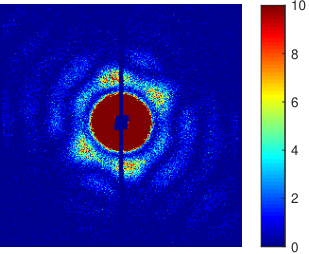
We stopped the EMC algorithm when the sum absolute differences of the two adjacent models was less than 0.001, and hence 41 EMC iterations were performed for $N_{3k}$ and 30 iterations for $N_{1k}$ . Figure 13 illustrated the sum absolute differences of the two adjacent 3D Fourier intensities. As can be seen, a peak appeared around the fifth EMC iteration for both datasets, suggesting the EMC algorithm has formed an icosahedron, and further iterations perfected the model. For synthetic dataset, EMC stopped after around 15 iterations.

Figure 13. The sum absolute differences of two EMC models from two adjacent iterations.

Appendix B Retrieved objects from Synthetic data

Let $W_{j}$ be the ground truth of a 2D diffracted pattern in the $j$ th rotation, i.e. $W_{j}$ can be simulated as a slice of a Fourier transformed particle through the particle center at the $j$ th rotation. If photon counting is a Poisson process, we may write the 2D diffraction patterns without background noise as $(K_{j}^{*})_{j=1}^{M}=Poisson(W_{j})$ , where $M$ is the number of sampled rotations, where $M=3000$ was used in our simulations. Considering a varying photon fluence, we write $K^{f}=Poisson(W\phi)$ , where $\phi$ is constant for all pixels in one pattern, but differs from shot to shot. For our synthetic data we took $\phi$ a uniform random number in the range $[0.9,1.1]$ . We also added a background signal, related to the X-ray beam configuration, i.e. $(K_{j}^{b})_{j=1}^{M}=Poisson(W_{j}\phi_{j}+K_{b})$ . Note that $K_{b}$ is a 2D pattern that is the same for all patterns under the same beam configuration, and we illustrate $K_{b}$ in Figure . Moreover, an extra source of scattering, was considered as $(K_{j}^{3})_{j=1}^{M}=Poisson(W_{j}\phi_{j}+K_{b}+B(p))$ , where $B$ takes the value 1 with probability $p=1000^{-1}$ , and zero otherwise, and we illustrate an example of $K_{b}+B(p)$ in Figure . Different real-space objects reconstructed from different datasets are shown in Figure 14.

Appendix C Background Subtraction

For given discrete shells $(s_{u})_{u=1}^{U}$ , let $S=(S_{u})_{u=1}^{U}$ be the radial shells of a 3D Fourier intensity $\mathbb{W}$ . The $u$ th shell is given by $S_{u}=\{s=(x,y,z);s_{u}\leq\|s\|<s_{u+1}\}$ , where $s$ is a point (voxel) at position $(x,y,z)$ , and $\|s\|$ is the Euclidean norm. The background noise in shell $u$ �is then estimated by

(10)

\displaystyle B_{u}=\beta\min_{s\in S_{u}}(\mathbb{W})_{s},

and we chose $\beta=0.5$ for our EMC reconstructions. We denote the average shell of a 3D Fourier intensity by

(11)

\displaystyle D_{u}=|S_{u}|^{-1}\sum_{s\in S_{u}}(\mathbb{W})_{s},

where $|S_{u}|$ is the number of voxels in the $u$ th shell. Note that $D_{u}$ can be also considered as the average power spectral density (PSD). The results of background subtraction showed larger contrasts and clear boundaries, see Figure 15.

The PSD profiles of $N_{1k}$ and $N_{3k}$ were similar, however, the Fourier intensity for $N_{1k}$ was coarser in the high frequencies, due to the lack of data to fill in the space, see Figure and Figure .