Analytical representation of Gaussian processes in the plane
Abstract
Closed-form expressions, parametrized by the Hurst exponent and the length of a time series, are derived for paths of fractional Brownian motion (fBm) and fractional Gaussian noise (fGn) in the plane, composed of the fraction of turning points and the Abbe value . The exact formula for is expressed via Riemann and Hurwitz functions. A very accurate approximation, yielding a simple exponential form, is obtained. Finite-size effects, introduced by the deviation of fGn’s variance from unity, and asymptotic cases are discussed. Expressions for for fBm, fGn, and differentiated fGn are also presented. The same methodology, valid for any Gaussian process, is applied to autoregressive moving average processes, for which regions of availability of the plane are derived and given in analytic form. Locations in the plane of some real-world examples as well as generated data are discussed for illustration.
I Introduction
The characterization and classification of time series Beran 1994; Brockwell and Davis 1996; Brockwell and Davis 2002; Beran et al. 2013 is an important task in a variety of fields. Several methods have been developed for tasks such as detecting chaos Hegger et al. 1999, measuring complexity via entropies Bandt and Pompe 2002; Maggs and Morales 2013; Ribeiro et al. 2017, estimating the Hurst exponent Simonsen et al. 1998; Carbone et al. 2004; Arianos and Carbone 2007, distinguishing chaotic from stochastic processes based on graph theory Lacasa and Toral 2010, and more. A connection between chaos and long range dependence was also established for low-dimensional chaotic maps Tarnopolski 2018.
The plane Tarnopolski 2016, spanned by the fraction of turning points and the Abbe value , was initially introduced to provide a fast and simple estimate of the Hurst exponent , as tight relations of both and with were discovered for fractional Brownian motion (fBm), fractional Gaussian noise (fGn), and differentiated fGn (DfGn). While and strongly overlap for for different processes, in the joint space the fBm and fGn intersect only at the point corresponding to white noise, i.e. . A few real-world data sets (monthly mean of the sunspot number (SSN); stock market indices; chaotic time series from the Lorenz system and the Chirikov map) were shown to lie firmly on the fBm branch. Moreover, the estimates of based on the empirical relation and computed using a wavelet method (Peng et al. 1994; Peng et al. 1995) were consistent with each other.
The discriminative power of the plane was demonstrated in a multiscale scheme Zunino et al. 2017a by employing coarse-grained sequences, i.e. dividing the time series into nonoverlapping segments of length and calculating the mean in each segment. This produces smoothed sequences, and the evolution of and with varying temporal scale allowed to separate (i) developed, emerging and frontier stock markets; (ii) healthy and epileptic patients based on their EEG recordings—moreover, for the first time it was possible to distinguish healthy patients with closed and open eyes; and (iii) patients with and without cardiac diseases based on the heart rate variabilty. Finally, it is also possible to differentiate between chaotic and stochastic processes based on the different behavior of paths, parametrized by , in the plane Zhao and Morales 2018. The plane is therefore a powerful tool with several possible applications.
The aim of this paper is to derive analytical descriptions of fBm and fGn, as well as autoregressive moving average (ARMA) processes, in the plane. In Sect. II the known facts about turning points are recapitulated. In Sect. III the exact and approximated expressions for are derived, for the first time, for fBm and fGn. Their plane’s representation is depicted in Sect. IV. ARMA processes are discussed in Sect. V. Various applications, ranging from pure mathematics, to biology and astrophysics, to financial markets, are briefly outlined in Sect. VI. Summary and concluding remarks with future prospects are gathered in Sect. VII.
II Fraction of turning points,
II.1 Theory
Consider three values of a time series . For the points are consecutive. Assume there are no ties between the neighboring points, which for continuous processes, or empirical data with decent resolution, should not be an issue (see also (Zunino et al. 2017b; Traversaro et al. 2018)). Three points can be arranged in six ways, identified by an order pattern (Fig. 1). If the smallest value among the three is given an index 1, and the largest an index 3, then e.g. the relation for one of the four possible turning points, , is described by a pattern . Denote the probability of encountering a pattern by . Then the following theorem holds Bandt and Shiha 2007:
Theorem 1
For a Gaussian process with stationary increments, , and the other patterns yield probability .
The probability for a given delay is given by
| (1) |
where the correlation coefficient is
| (2) |
The probability of encountering a turning point among three consecutive points (i.e., for , the case considered hereinafter), as per Theorem 1, is then
| (3) |
Note that : zero is attained by monotonic sequences, while unity is (asymptotically) achieved for strictly alternating time series. For an uncorrelated process all patterns are equally probable, hence . Further details on order patterns can be found in Bandt and Shiha 2007.
II.2 for fBm, fGn, and DfGn
With the following properties of fBm , fGn , and DfGn , one can utilize the methodology from Sect. II.1 to calculate for them as a function of :
| (4a) | ||||
| (4b) | ||||
| (4c) | ||||
| (4d) | ||||
| (4e) | ||||
| (4f) | ||||
Eq. (4c) and (4d) can be obtained from Eq. (4a) and (4b) by substituting ; likewise, Eq. (4e) and (4f) follow from Eq. (4c) and (4d) by using . 11 1 In the derivation of and one can actually employ only the relations for fBm; the calculations would then become quite burdensome, though.
For fBm, one has
| (5) |
which is roughly equal to from Tarnopolski 2016, where is the number of turning points in a time series of length Brockwell and Davis 1996; Kendall and Stuart 1973, and is the expected value for white noise 22 2 The first and last points cannot form a turning point, hence the subtraction of 2 in .. In general, . The plot of Eq. (5) is shown in Fig. 2, together with data simulated as in Tarnopolski 2016 (scaled herein from to ). For an fGn:
| (6) |
and for the increments of fGn, i.e. DfGn:
| (7) |
both of which are also shown in Fig. 2.

III Abbe value,
The Abbe value of a time series is defined as half the ratio of the mean-square successive difference to the variance Tarnopolski 2016; von Neumann 1941a; von Neumann 1941b; Kendall 1971; Mowlavi 2014:
| (8) |
It quantifies the smoothness (raggedness) of a time series by comparing the sum of the squared differences between two successive measurements with the variance of the whole time series. It decreases to zero for time series displaying a high degree of smoothness, while the normalization factor ensures that tends to unity for a white noise process Williams 1941. It was proposed as a test for randomness (Bingham and Nelson 1981; Bartels 1982; Mateus and Caeiro 2018). It is straightforward to show that for a 2-periodic time series, , , while for a 3-periodic one, , .
Consider to be a realization of length of an fBm, , with Hurst exponent . Thence, its increments form an fGn, , with the same . One can then express as
| (9) |
where the dependence on and is highlighted. Similarly, for an fGn
| (10) |
where is the corresponding DfGn, i.e. the increments of fGn, . The goal is to calculate the variances of , , and .
III.1 Variance of fGn
We start with since it occurs in both Eq. (9) and (10). The same methodology that was used in Delignières 2015 to calculate is employed, i.e.
| (11) | ||||
Developing the sum for a few values of , and utilizng the variance and covariance from Eq. (4c) and (4d), one can observe a pattern emerging, that leads to a formula:
| (12) |
It yields
| (13) |
i.e. it asymptotically approaches Eq. (4c). However, for finite , . The plot of Eq. (12) for is shown in Fig. 3. For values the departure from the asymptotic value becomes significant.
III.2 Variance and Abbe value of fBm
The variance of the discrete, finite length is given in Delignières 2015 as
| (14) |
For , ; then , so , hence, per Eq. (9) and given Eq. (12), , i.e. asymptotically approaches unity.
Using the symbolic computer algebra system Mathematica one can calculate the sum in Eq. (14) to be 33 3 See also www.wolframalpha.com.
| (15) |
where is the Riemann , and is the Hurwitz Apostol 1976. Hence, taking into account Eq. (12), one can give a closed-form formula:
| (16) |
which, since , , , and , yields .
In order to provide a simpler, approximate expression for , first observe that since at and for the ratio of the Hurwitz terms and the Riemann terms is big, i.e.
| (17) |
and that for this ratio is monotonically increasing (Fig. 4), therefore
| (18) |
hence is a negligible contribution, so it does not need to be taken into account.
Let us express as a globally convergent Newton series, i.e. utilize the Hasse representation Hasse 1930:
| (19) |
valid for , . The first term of the outer sum, i.e. for and at , is
| (20) |
The second term, i.e. for , is
| (21) |
And similarly for higher . Therefore, for one obtains an approximation
| (22) |
and for :
| (23) |
but since , , so one also obtains
| (24) |
For higher , although given that , one has , hence yielding the same approximation. Indeed, is the Kronecker , , hence only the term survives. For one obtains a similar expression:
| (25) |
Therefore, with these approximations one can write:
| (26) |
so that
| (27) |
and since , one finally obtains
| (28) |
and
| (29) |
which also yields , asymptotically approaching unity. In case one sets , the simplest approximation is then obtained as
| (30) |
These various approximations of are shown in Fig. 5. For an unreasonably small one sees discrepancies between the curves for low and moderate , although they are rather small. The finite-size effects, introduced by from Eq. (12), are significant at higher values of . For a moderate , the curves are indistinguishable for most of the range of , with the region of significant influence of moved systematically to higher , and for even longer time series (e.g. ) the consistency of all curves is only strengthened. Therefore, the approximation from Eq. (30) is a decent one for time series with any reasonable length.
III.3 Variance of DfGn and Abbe value of fGn
To obtain an expression for the same methodology from Sect. III.1 is undertaken, i.e. Eq. (11) with changed to is employed. Again, developing the sum for a few values of , and utilizng the variance and covariance from Eq. (4e) and Eq. (4f), one can observe the pattern depicted in Table 1. Hence one can write
| (31) |
The exact expression for the Abbe value, taking into account Eq. (12), is thence
| (32) |
In the limit , i.e. for any reasonable , Eq. (31) becomes
| (33) |
i.e. it asymptotically approaches Eq. (4e). Plots of Eq. (31) and (33) are shown in Fig. 6. For very short time series there is a certain deviation between the expressions, but for higher the difference is invisible. Therefore, the asymptotic Eq. (33) is adequate in any practical scenario.
| 2 | |||||
|---|---|---|---|---|---|
| 3 | |||||
| 4 | |||||
| 5 | |||||
| 6 | |||||
| 7 | |||||
| 8 | |||||
| 9 | |||||
| 10 | |||||
The Abbe value is thence
| (34) |
As discussed in Sect. III.1, the variance of can in some instances be approximated by unity. Eq. (34) simplifies then to just
| (35) |
independent on the length of the time series.
The asymptotic Eq. (35) ranges from to when decreases from 1 to 0. The expression from Eq. (34) reaches its maximum of at . The asymptotic minimum, as , is . For , these values are 1.49991 and 0.14285, respectively, in perfect agreement with Fig. 3 in Tarnopolski 2016.
IV Representation of fBm and fGn in the plane
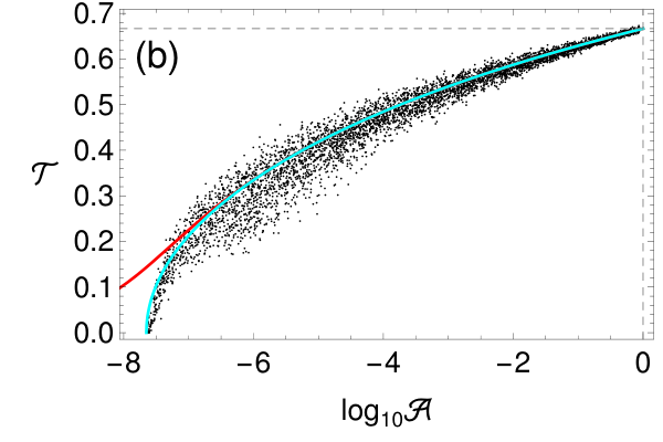
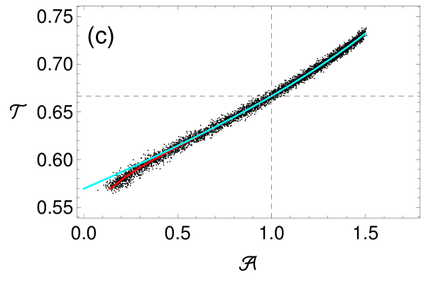
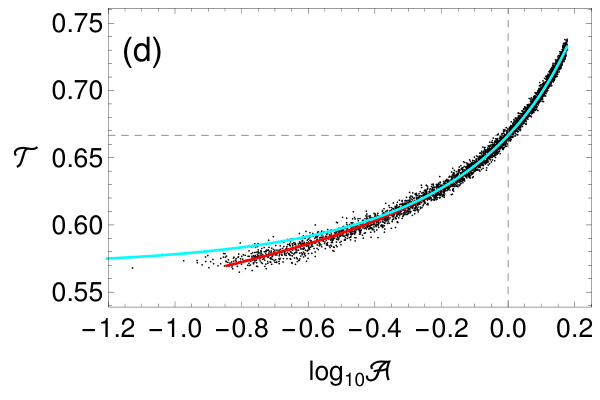
The plane is displayed in Fig. 7. The black points come from simulations Tarnopolski 2016. In case of fBm [Fig. 7 (a) and (b)], the red line employs the exact formula for from Eq. (16), while the cyan line depicts the approximation from Eq. (30). Eq. (5) describes .
In case of fGn [Fig. 7 (c) and (d)], the red line corresponds to the exact Eq. (32) for , while the cyan line to the asymptotic form from Eq. (35). Eq. (6) describes . Panels (b) and (d) of Fig. 7 employ a logarithmic horizontal axis to fully display the dependence at small values of (i.e. high values of ). The agreement between numerical simulations and the analytic description is very good; also the approximations for work well in the plane. In particular, the approximation from Eq. (34) for fGn is as good as the exact Eq. (32).
V ARMA processes
The methodology from Sect. II and III is applicable also to ARMA processes. Generalizing Eq. (8), similarly as was done in Eq. (9) and (10), the Abbe value of a process is
| (36) |
where denotes the increments of . The fraction of turning points is given by Eq. (1)–(3). It will be convenient to express in terms of the autocorrelation function :
| (37) |
so that Eq. (1) becomes
| (38) |
This formula can be directly applied also to fGn and DfGn, but not to fBm which is nonstationary.
For ARMA processes, and are easily obtainable Brockwell and Davis 1996; Brockwell and Davis 2002. The variance of the differentiated process, , is calculated as
| (39) |
V.1 AR(1)
Consider a weakly stationary process , , where is a white-noise error term. Then
| (40) |
for all , thus
| (41) |
reaching its minimum of when , and its maximum of when .
One then obtains
| (42) |
and
| (43) |
and thus
| (44) |
reaching its minimum of when , and maximum of when . One can then write explicitly as a function of :
| (45) |
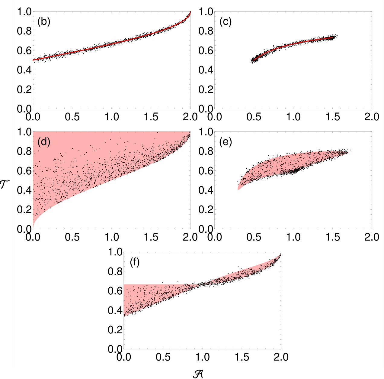
which is displayed in Fig. 8. The Ornstein-Uhlenbeck (OU) process, a continuous analog of AR(1), yields the same Eq. (45), but restricted to (see Appendix A).
V.2 AR(2)
Consider a weakly stationary process , . Then is given by a recurrent relation (the Yule-Walker equations):
| (46) |
thus
| (47) |
reaching its minimum of when , and its maximum of along the line .
One then obtains
| (48) |
and
| (49) |
thus
| (50) |
reaching its minimum of along the line , and maximum of along the line . One cannot write explicitly as a function of , as is a two-dimensional region, depicted in Fig. 8. However, it is possible to give a simple formula for the boundaries of this region. Note that for a given , is minimal when . Hence by setting , one can then solve Eq. (50) for , i.e. write , and insert this into Eq. (47) to obtain the lower boundary as
| (51) |
The upper boundary, , is attained when , and from the left the region is a vertical line , obtained by sweeping from to .
Notice that AR(1) is a special case of AR(2) with . One can then observe, by repeating the above reasoning for an arbitrary , that the region of availability, , is formed as a continuum of curves parametrized by :
| (52) |
reducing to Eq. (51) when .
V.3 MA(1)
Consider , weakly stationary for all . The autocorrelation function is
| (53) |
thus
| (54) |
reaching its minimum of at , and its maximum of at .
One then obtains
| (55) |
and
| (56) |
thus
| (57) |
reaching its minimum of at , and maximum of at . One can then write explicitly as a function of :
| (58) |
which is displayed in Fig. 8.
V.4 MA(2)
Consider , weakly stationary for all , for which
| (59) |
thus
| (60) |
reaching its minimum of at , and its maximum of at .
One then obtains
| (61) |
and
| (62) |
thus
| (63) |
reaching its minimum of at , and maximum of at . One cannot write explicitly as a function of , as is a two-dimensional region, depicted in Fig. 8.
V.5 ARMA(1,1)
Consider , weakly stationary for and all , for which
| (64) |
thus
| (65) |
reaching its minimum of when , and its maximum of when , along the line .
One then obtains
| (66) |
and
| (67) |
thus
| (68) |
reaching its minimum of when , along the line , and maximum of when , along the line . One cannot write explicitly as a function of , as is a two-dimensional region, depicted in Fig. 8.
Note that Eq. (65) and (68) are invariant on changing to , so that in the context of geometrical depiction of the region of availability only the range needs to be considered. Roughly speaking, cases with are equivalent to . However, are special instances:
- •
when , Eq. (68) yields , which fulfills the stationarity condition, , only for . In this range:
(69) - •
likewise, when , one obtains , which leads to , giving:
(70)
In particular, reduces an ARMA(1,1) process to an AR(1) one, reproducing respective formulae from Sect. V.1.
Similarly as was done in Sect. V.2 for AR(2) processes, the region of availabity for ARMA(1,1) can be described as a continuum of curves, , parametrized by : one needs to solve Eq. (68) for and insert the solution into Eq. (65). The resulting formula, easy to derive but of a quite complicated and noninformative form, is not displayed herein.
VI Applications
VI.1 Bacterial cytoplasm
The two-dimensional motion of individual mRNA molecules inside live Escherichia coli bacteria were tracked in (Golding and Cox 2006). It was found that they follow anomalous diffusion, with , confirmed by other methods as well (Magdziarz et al. 2009). Herein, the time series and are treated separately. Results for the 27 tracks are displayed in Fig. 9 for the -axis. Similar outcomes were obtained for the -axis. The locations in the plane are in agreement with an fBm description, and the values extracted using Eq. (5) and (30), yielding , are consistent with each other, and confirm that the observed process is indeed subdiffusive.
VI.2 Zeros of the Riemann
The first nontrivial zeros, , of the Riemann function (Platt 2015) were retrieved 44 4 https://www.lmfdb.org/zeros/zeta/. Normalized spacings between consecutive zeros were computed as (Odlyzko 1987)
| (71) |
The location of this sequence in the plane is . This is remarkably close to the fGn line (Fig. 10), and Eq. (6) and (35) give . In comparison, the discrete wavelet transform (DWT) method (Tarnopolski 2016) returns , hence also strongly implying . However, as the distribution of is not normal, but rather follows the distribution of the Gaussian unitary ensemble (GUE) according to the GUE hypothesis (Montgomery 1973), so this sequence is not a Gaussian process, strictly speaking. Note, however, that a location in the plane can be computed for any type of data; in this case, due to and , one gets a clear information that the series is—in a sense—(much) more noisy than regular white noise.
VI.3 Sunspot numbers
The curently available from the World Data Center Sunspot Index and Long-term Solar Observations 55 5 SILSO World Data Center, Royal Observatory of Belgium, Brussels, http://www.sidc.be/silso sample of 3250 monthly SNN are described by , as computed with the DWT approach 66 6 Similar value can be obtained with data in (Tarnopolski 2016) when the two outliers on the left of Fig. 6b therein are discarded.. The location in the plane is , Fig. 10, and Eq. (5) and (30) give . This is in agreement with some works (Movahed et al. 2006) that also compute . Note that the SSN sequence is slightly off the fBm line, hence it not necessarily need to be adequately modeled by an fBm process. The SSN is a straightforward way of monitoring the Sun’s activity, and since the sunspots are tightly connected with the magnetic fields governing solar flares and coronal mass ejections, its proper modeling is crucial in forecasting the space weather conditions.
VI.4 Chaos
The Chirikov standard map for a chaotic state (in an unbounded setting) was examined in (Tarnopolski 2016). Its location in the plane is , and lies directly on the fBm line, Fig. 10, and Eq. (5) and (30) give , which is in perfect agreement with the estimate with DWT method, yielding . This means that, in the context of long-term memory, it is uncorrelated, and acts like Brownian motion.
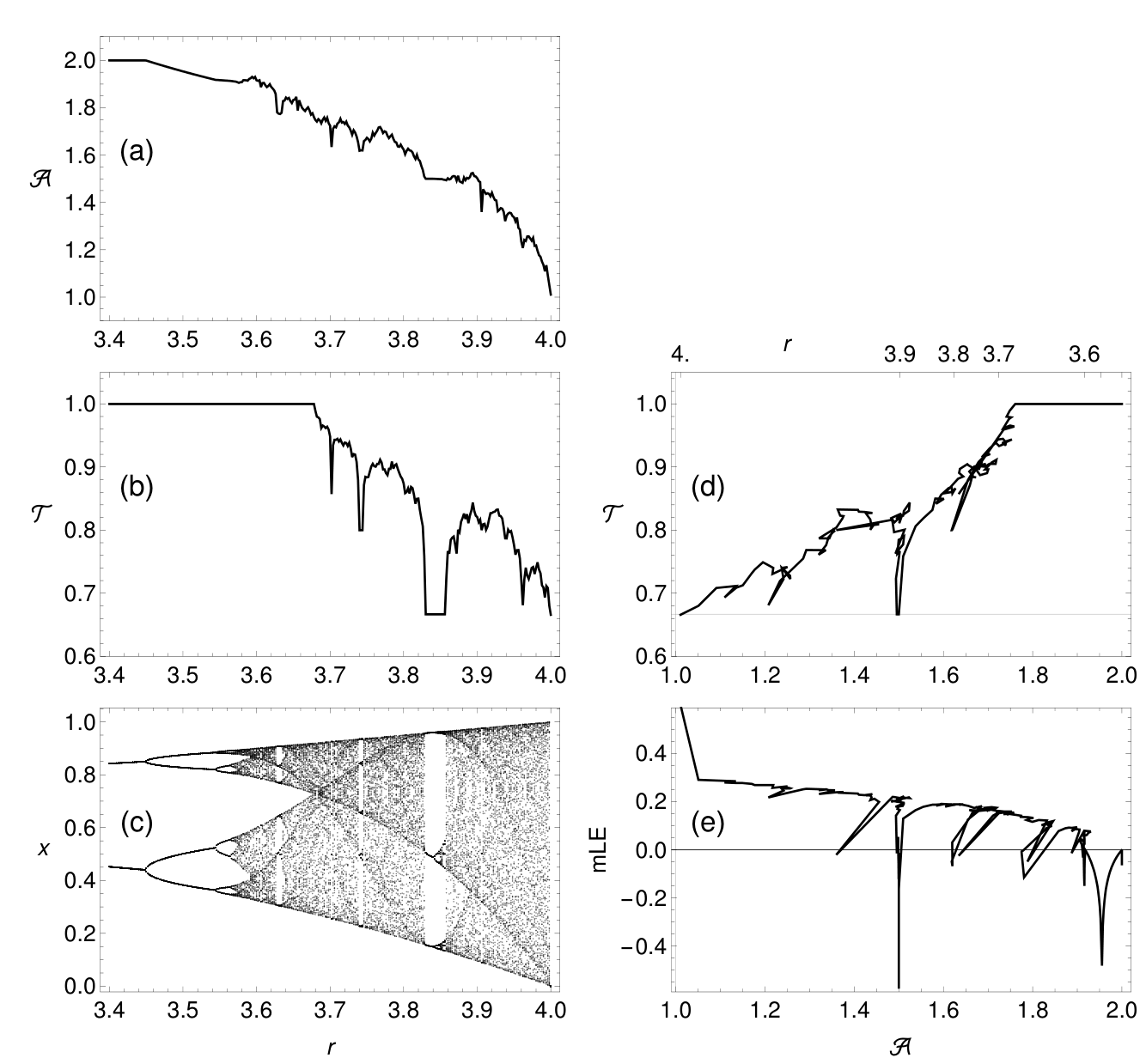
To further illustrate chaotic behavior in the plane, the logistic map is considered. For , with a step , time series of length were generated and their locations, as well as the maximal Lyapunov exponents (mLEs), were computed. The dependencies of and on , the bifurcation diagram, the plane, and the relation between and mLE, are shown in Fig. 11. When chaos is most developed (), the trajectories approach the point , identical for white noise [Fig. 11(d)]. Hints that fully developed chaos behaves this way were noted in case of the Lorenz system (Tarnopolski 2016; Zunino et al. 2017a). With increasing , a gradual decrease in occurs, with wells in periodic windows [Fig. 11(b)]. Note that up to , because apparently the orbits, even when chaotic, are strictly alternating. is more sensitive to changes in dynamics, as for period-2 orbits (see the beginning of Sect. III) before the bifurcation at , and then systematically decreases in the period-4 window before the next bifurcation at [Fig. 11(a)]. There are also shallow wells at periodic windows within the chaotic zone. The path in the plane is jagged, and various changes in dynamics are manifested, corresponding to changes in mLEs [Fig. 11(e)] and in the bifurcation diagram [Fig. 11(c)].
A tight, positive correlation between mLE and for the Chirikov map was discovered (Tarnopolski 2018) (see also (Steeb and Andrieu 2005)). Differences between (quasi)periodic and chaotic systems were observed in the coarse-grained sequences in the plane in case of a sinusoidally driven thermostat (Zhao and Morales 2018). These connections between chaos, , and the plane are nontrivial, and require further research. Describing a universal (if existent) behavior of chaotic systems in the plane in an interesting perspective. The possibility of differentiating between chaotic and stochastic time series is a hopefully attainable application.
VI.5 Markets
The efficient market hypothesis (Mantegna and Stanley 2000) is a key concept in finance. If a market exhibits , then it might allow arbitrage. A classification of developed, emerging and frontier stock markets in the plane was performed in (Zunino et al. 2017a), and showed that these three categories of markets occupy distinct regions of the space. Hence, the plane is a useful tool for classifying data with different underlying dynamics.
The time evolution of of many stock markets shows it is oscillating around (Carbone et al. 2004). Similarly, one can investigate how and evolve, and hence trace their values in the plane at different times. As an example consider the Warsaw Stock Exchange Index (Warszawski Indeks Giełdowy, WIG) 77 7 https://www.investing.com/indices/wig-historical-data, accessed on November 10, 2019. Its location in the plane, right on the fBm line, is depicted in Fig. 10, and the estimates of , obtained by solving Eq. (5) and (30) with , yield . The DWT method returns . The time evolution is depicted in Fig. 12. It is obtained by partitioning the whole time series into overlapping segments of size , advancing each segment by one point. Throughout its history, the WIG remains confined in a small region of the plane.
VI.6 Active galactic nuclei
A core focus in astronomy is the investigation of apparent variability of various celestial objects such as asteroids, stars, or galaxies. Within the latter, of particular interest are active galactic nuclei (AGNs), further divided into several types (Urry and Padovani 1995). Among them, blazars are peculiar AGNs pointing their relativistic jets toward the Earth. Blazars are commonly divided further into two subgroups, i.e. flat spectrum radio quasars (FSRQs) and BL Lacertae (BL Lac) objects, based on characteristics visible in their optical spectra. In a recent study (Żywucka et al. 2019) it was found that faint FSRQ and BL Lac candidates located behind the Magellanic Clouds are clearly separated in the plane, with means of and , respectively. This differentiation, based solely on the temporal data in the form of light curves, is another proof that employing the plane as a classification tool is a promising approach.
VI.7 Other
The worked-out examples from Sect. VI.1–VI.6 do not exhaust the possible applications of the plane in regard to constraining the value of , or classifying time series. Some other interesting instances include, but are not restricted to: ferro- and paramagnetic states of the Heisenberg model that exhibit and , respectively (Zhang et al. 1993), and should be easily distinguishable in the plane; a photonic integrated circuit yields for varied electric field of the feedback, coupled with chaotic behavior (Chlouverakis et al. 2008); cataclysmic variable stars observed in X-rays exhibit long-term memory, , suggesting the accretion is driven by magnetic fields (Anzolin et al. 2010); football matches can follow the rules of fBm with (Kijima et al. 2014); persistence of amoeboid motion (Makarava et al. 2014) as well as Nitzschia sp. diatoms (Murguía et al. 2015); Solar wind proton density fluctuations are characterized by , placing constraints on the models of kinetic turbulence (Carbone et al. 2018); values were computed for epileptic patients’ brain activity, quantified via magnetoencephalographic recordings, and appear to be a promising additional diagnostic tool for identifying epileptogenic zones in presurgical evaluation (Witton et al. 2019). Recall that epilepsy has been already investigated in the plane as well (Zunino et al. 2017a).
VII Summary and open questions
Exact analytical descriptions for the locations of fBm and fGn in the plane were derived. Working approximations were also obtained in the following forms:
and
and were demonstrated to be adequate for time series with any reasonable length . This allows to classify time series of any length, respective to fBm and fGn, without relying on time-consuming numerical simulations. These analyses add to the theoretical results regarding fBm and fGn (Zunino et al. 2008; Sadhu et al. 2018). The same methodology was applied to ARMA processes. Analytic descriptions of the available regions of the plane were derived and illustrated for .
Further research on is required, as it has been rarely utilized, with some recent, nonextensive examples in astronomy (Shin et al. 2009; Mowlavi 2014; Sokolovsky et al. 2017; Pérez-Ortiz et al. 2017; Żywucka et al. 2019) (but see also (Lafler and Kinman 1965)). The interrelations between ordinal patterns, persistence, and chaos (Zanin et al. 2012; Ribeiro et al. 2017) are linked even tighter with the bidimensional scheme of the plane. The presented methodology is valid for any Gaussian process, but it should be emphasized that the locations can be computed for arbitrary time series, serving e.g. as classification or clustering methods for empirical data.
Naturally, a question about representations of other stochastic processes arises. Examples include the following:
- •
Representation of colored noise, i.e. power spectral densities (PSDs) of the form . fBm can be associated with , and fGn is characterized by . However, power laws are ubiquituous in nature, hence their locations in the plane, for any , is an interesting and challenging problem.
- •
In some fields, e.g. in astronomy, the observed signals often yield PSDs of the form , where is the so called Poisson noise level, coming from the statistical noise due to uncertainties in the measurements; above a certain frequency, the PSD transitions from a power law to white noise. A representation of such processes in the plane is crucial in classifying light curves of several sources, e.g. AGN.
- •
Other continuous-time models, e.g. continuous ARMA (Brockwell 2014), have been developed. The simplest in this family is the OU process, which is a continuous analog of the AR(1) process, with the same representation. Introducing long-term memory leads to continuous autoregressive fractionally integrated moving average models (Tsai 2009).
Acknowledgements.
The author thanks Ido Golding for providing the data of the mRNA motion inside the bacteria. Support by the Polish National Science Center through OPUS Grant No. 2017/25/B/ST9/01208 is acknowledged.*
Appendix A Ornstein-Uhlenbeck process
References
- Beran (1994) J. Beran, Statistics for Long Memory Processes (Chapman and Hall, New York, 1994).
- Brockwell and Davis (1996) P. J. Brockwell and R. A. Davis, Time Series: Theory and Methods, 2nd ed. (Springer-Verlag New York, 1996).
- Brockwell and Davis (2002) P. J. Brockwell and R. A. Davis, Introduction to Time Series and Forecasting, 2nd ed. (Springer-Verlag New York, 2002).
- Beran et al. (2013) J. Beran, Y. Feng, S. Ghosh, and R. Kulik, Long Memory Processes: Probabilistic Properties and Statistical Methods (Springer-Verlag, Berlin Heidelberg, 2013).
- Hegger et al. (1999) R. Hegger, H. Kantz, and T. Schreiber, Chaos 9, 413 (1999).
- Bandt and Pompe (2002) C. Bandt and B. Pompe, Physical Review Letters 88, 174102 (2002).
- Maggs and Morales (2013) J. E. Maggs and G. J. Morales, Plasma Physics and Controlled Fusion 55, 085015 (2013).
- Ribeiro et al. (2017) H. V. Ribeiro, M. Jauregui, L. Zunino, and E. K. Lenzi, Physical Review E 95, 062106 (2017).
- Simonsen et al. (1998) I. Simonsen, A. Hansen, and O. M. Nes, Physical Review E 58, 2779 (1998), cond-mat/9707153 .
- Carbone et al. (2004) A. Carbone, G. Castelli, and H. E. Stanley, Physica A: Statistical Mechanics and its Applications 344, 267 (2004).
- Arianos and Carbone (2007) S. Arianos and A. Carbone, Physica A: Statistical Mechanics and its Applications 382, 9 (2007).
- Lacasa and Toral (2010) L. Lacasa and R. Toral, Physical Review E 82, 036120 (2010).
- Tarnopolski (2018) M. Tarnopolski, Physica A: Statistical Mechanics and its Applications 490, 834 (2018).
- Tarnopolski (2016) M. Tarnopolski, Physica A: Statistical Mechanics and its Applications 461, 662 (2016).
- Peng et al. (1994) C.-K. Peng, S. V. Buldyrev, S. Havlin, M. Simons, H. E. Stanley, and A. L. Goldberger, Physical Review E 49, 1685 (1994).
- Peng et al. (1995) C.-K. Peng, S. Havlin, H. E. Stanley, and A. L. Goldberger, Chaos 5, 82 (1995).
- Zunino et al. (2017a) L. Zunino, F. Olivares, A. F. Bariviera, and O. A. Rosso, Physics Letters A 381, 1021 (2017a).
- Zhao and Morales (2018) Y. Zhao and G. J. Morales, Physical Review E 98, 022213 (2018).
- Zunino et al. (2017b) L. Zunino, F. Olivares, F. Scholkmann, and O. A. Rosso, Physics Letters A 381, 1883 (2017b).
- Traversaro et al. (2018) F. Traversaro, F. O. Redelico, M. R. Risk, A. C. Frery, and O. A. Rosso, Chaos 28, 075502 (2018).
- Bandt and Shiha (2007) C. Bandt and F. Shiha, Journal of Time Series Analysis 28, 646 (2007).
- (22) In the derivation of and one can actually employ only the relations for fBm; the calculations would then become quite burdensome, though.
- Kendall and Stuart (1973) M. Kendall and A. Stuart, The advanced theory of statistics (London: Griffin, 3rd ed., 1973).
- (24) The first and last points cannot form a turning point, hence the subtraction of 2 in .
- Sinn and Keller (2008) M. Sinn and K. Keller, arXiv e-prints , arXiv:0801.1598 (2008), arXiv:0801.1598 [math.PR] .
- von Neumann (1941a) J. von Neumann, The Annals of Mathematical Statistics 12, 153 (1941a).
- von Neumann (1941b) J. von Neumann, The Annals of Mathematical Statistics 12, 367 (1941b).
- Kendall (1971) M. G. Kendall, Biometrika 58, 369 (1971).
- Mowlavi (2014) N. Mowlavi, Astronomy & Astrophysics 568, A78 (2014).
- Williams (1941) J. D. Williams, The Annals of Mathematical Statistics 12, 239 (1941).
- Bingham and Nelson (1981) C. Bingham and L. S. Nelson, Technometrics 23, 285 (1981).
- Bartels (1982) R. Bartels, Journal of the American Statistical Association 77, 40 (1982).
- Mateus and Caeiro (2018) A. Mateus and F. Caeiro, “Exact and approximate probabilities for the null distribution of bartels randomness test,” in Recent Studies on Risk Analysis and Statistical Modeling, edited by T. A. Oliveira, C. P. Kitsos, A. Oliveira, and L. Grilo (Springer International Publishing, Cham, 2018) pp. 227–240.
- Delignières (2015) D. Delignières, Mathematical Problems in Engineering 2015, 485623 (2015).
- (35) See also www.wolframalpha.com.
- Apostol (1976) T. M. Apostol, Introduction to Analytic Number Theory (Springer Science+Business Media New York, 1976).
- Hasse (1930) H. Hasse, Mathematische Zeitschrift 32, 458 (1930).
- Golding and Cox (2006) I. Golding and E. C. Cox, Physical Review Letters 96, 098102 (2006).
- Magdziarz et al. (2009) M. Magdziarz, A. Weron, K. Burnecki, and J. Klafter, Physical Review Letters 103, 180602 (2009).
- Platt (2015) D. J. Platt, Mathematics of Computation 84, 1521 (2015).
- (41) https://www.lmfdb.org/zeros/zeta/.
- Odlyzko (1987) A. M. Odlyzko, Mathematics of Computation 48, 273 (1987).
- Montgomery (1973) H. L. Montgomery, in Analytic number theory, Proc. Sympos. Pure Math., XXIV, Providence, R.I.: American Mathematical Society, Vol. 24, edited by H. G. Diamond (1973) pp. 181–193.
- (44) SILSO World Data Center, Royal Observatory of Belgium, Brussels, http://www.sidc.be/silso.
- (45) Similar value can be obtained with data in (Tarnopolski 2016) when the two outliers on the left of Fig. 6b therein are discarded.
- Movahed et al. (2006) M. S. Movahed, G. R. Jafari, F. Ghasemi, S. Rahvar, and M. R. R. Tabar, Journal of Statistical Mechanics: Theory and Experiment 2006, P02003 (2006).
- Steeb and Andrieu (2005) W.-H. Steeb and E. C. Andrieu, Zeitschrift Naturforschung Teil A 60, 252 (2005).
- Mantegna and Stanley (2000) R. N. Mantegna and H. E. Stanley, An Introduction to Econophysics: Correlations and Complexity in Finance (Cambridge University Press, New York, 2000).
- (49) https://www.investing.com/indices/wig-historical-data, accessed on November 10, 2019.
- Urry and Padovani (1995) C. M. Urry and P. Padovani, Publications of the Astronomical Society of the Pacific 107, 803 (1995).
- Żywucka et al. (2019) N. Żywucka, M. Tarnopolski, M. Böttcher, Ł. Stawarz, and V. Marchenko, arXiv e-prints , arXiv:1912.03530 (2019), arXiv:1912.03530 [astro-ph.GA] .
- Zhang et al. (1993) Z. Zhang, O. G. Mouritsen, and M. J. Zuckermann, Physical Review E 48, R2327 (1993).
- Chlouverakis et al. (2008) K. E. Chlouverakis, A. Argyris, A. Bogris, and D. Syvridis, Physical Review E 78, 066215 (2008).
- Anzolin et al. (2010) G. Anzolin, F. Tamburini, D. de Martino, and A. Bianchini, Astronomy and Astrophysics 519, A69 (2010), arXiv:1005.5319 [astro-ph.SR] .
- Kijima et al. (2014) A. Kijima, K. Yokoyama, H. Shima, and Y. Yamamoto, European Physical Journal B 87, 41 (2014), arXiv:1402.0912 [physics.pop-ph] .
- Makarava et al. (2014) N. Makarava, S. Menz, M. Theves, W. Huisinga, C. Beta, and M. Holschneider, Physical Review E 90, 042703 (2014).
- Murguía et al. (2015) J. S. Murguía, H. C. Rosu, A. Jimenez, B. Gutiérrez-Medina, and J. V. García-Meza, Physica A: Statistical Mechanics and its Applications 417, 176 (2015), arXiv:1410.3135 [q-bio.QM] .
- Carbone et al. (2018) F. Carbone, L. Sorriso-Valvo, T. Alberti, F. Lepreti, C. H. K. Chen, Z. Němeček, and J. Šafránková, Astrophysical Journal 859, 27 (2018), arXiv:1804.02169 [physics.space-ph] .
- Witton et al. (2019) C. Witton, S. V. Sergeyev, E. G. Turitsyna, P. L. Furlong, S. Seri, M. Brookes, and S. K. Turitsyn, Journal of Neural Engineering 16, 056019 (2019).
- Zunino et al. (2008) L. Zunino, D. G. Pérez, M. T. Martín, M. Garavaglia, A. Plastino, and O. A. Rosso, Physics Letters A 372, 4768 (2008).
- Sadhu et al. (2018) T. Sadhu, M. Delorme, and K. J. Wiese, Phys. Rev. Lett. 120, 040603 (2018).
- Shin et al. (2009) M.-S. Shin, M. Sekora, and Y.-I. Byun, Monthly Notices of the Royal Astronomical Society 400, 1897 (2009).
- Sokolovsky et al. (2017) K. V. Sokolovsky, P. Gavras, A. Karampelas, S. V. Antipin, I. Bellas-Velidis, P. Benni, A. Z. Bonanos, A. Y. Burdanov, S. Derlopa, D. Hatzidimitriou, A. D. Khokhryakova, D. M. Kolesnikova, S. A. Korotkiy, E. G. Lapukhin, M. I. Moretti, A. A. Popov, E. Pouliasis, N. N. Samus, Z. Spetsieri, S. A. Veselkov, K. V. Volkov, M. Yang, and A. M. Zubareva, Monthly Notices of the Royal Astronomical Society 464, 274 (2017).
- Pérez-Ortiz et al. (2017) M. F. Pérez-Ortiz, A. García-Varela, A. J. Quiroz, B. E. Sabogal, and J. Hernández, Astronomy & Astrophysics 605, A123 (2017).
- Lafler and Kinman (1965) J. Lafler and T. D. Kinman, Astrophysical Journal Supplement 11, 216 (1965).
- Zanin et al. (2012) M. Zanin, L. Zunino, O. A. Rosso, and D. Papo, Entropy 14, 1553 (2012).
- Brockwell (2014) P. J. Brockwell, Annals of the Institute of Statistical Mathematics 66, 647 (2014).
- Tsai (2009) H. Tsai, Bernoulli 15, 178 (2009).