Evidence for Non-smooth Quenching in Massive Galaxies at –2019
Abstract
We investigate a large sample of massive galaxies at with combined HST broad-band and grism observations to constrain the star-formation histories of these systems as they transition from a star-forming state to quiescence. Among our sample of massive () galaxies at , dust-corrected and UV star-formation indicators agree with a small dispersion ( dex) for galaxies on the main sequence, but diverge and exhibit substantial scatter ( dex) once they drop significantly below the star-forming main sequence. Significant emission is present in galaxies with low dust-corrected UV SFR values as well as galaxies classified as quiescent using the diagram. We compare the observed flux distribution to the expected distribution assuming bursty or smooth star-formation histories, and find that massive galaxies at are most consistent with a quick, bursty quenching process. This suggests that mechanisms such as feedback, stochastic gas flows, and minor mergers continue to induce low-level bursty star formation in massive galaxies at moderate redshift, even as they quench.
Keywords:
galaxies: formation, evolution, starburst, high-redshift, ISM, ultraviolet: galaxies1 Introduction
A growing consensus of observations indicates that the population of massive quiescent galaxies has been building up since before (Bell et al. 2004; Faber et al. 2007; Ilbert et al. 2013). The presence of this population at early epochs poses a significant challenge to our current understanding of galaxy formation and evolution, as these systems must have formed early and suffered a quick shutdown in star formation (Peng et al. 2010; Thomas et al. 2010; Kuntschner et al. 2010; van Dokkum et al. 2015; Daddi et al. 2005; Goddard et al. 2017, ‘quenching’;). Many mechanisms have been proposed to cause this shutdown of star formation in massive galaxies, such as the build-up of a hot-gas halo (Kereš et al. 2005; Dekel & Birnboim 2006), feedback from an Active-Galactic-Nucleus (Di Matteo et al. 2005; Hopkins et al. 2006; Beckmann et al. 2017, AGN;) or star formation activity (Oppenheimer & Davé 2006; Ceverino & Klypin 2009) driven by a recent merger (Hopkins et al. 2014), or the stabilization of the cold gas against fragmentation (Martig et al. 2009). However, the importance/feasibility of these processes, and how they may evolve with redshift, is still uncertain and remains a major unanswered question in our current understanding of galaxy evolution.
As many authors have noted (Martin et al. 2007; Schawinski et al. 2014; Wild et al. 2016; Belfiore et al. 2016; Pandya et al. 2017), understanding of the processes involved in quenching can be discerned through detailed studies of massive galaxies in the process of transitioning from star-forming to quiescent. Determining the star-formation histories of these galaxies can constrain which processes drive quenching. For example, Schawinski et al. 2007 found that local early-type galaxies are consistent with a short ( Myr) quenching associated with merger-driven feedback, but late-type galaxies are consistent with a longer (many Gyr) quenching process such the buildup of a hot gas halo through radio-mode AGN feedback (Croton et al. 2006). Similarly, by using semi-analytic models describing the star-formation histories of massive galaxies, Pandya et al. 2017 found that a fast quenching mode is the predominant quenching mode at high , whereas low- galaxies are associated with a slower quenching process. At , Zick et al. 2018 investigate the spectra of transition galaxies at, finding that quenching occurs on a Myr timescale, and using photometric data of galaxies between and , Carnall et al. 2018 find that most massive galaxies are consistent with quenching times Gyr. Studies investigating the abundance of galaxies with SFRs in between the star-forming and quiescent populations over cosmic time find that quenching takes place on Gyr timescales (Wetzel et al. 2013; Balogh et al. 2004; Hahn et al. 2017).
However, the photometric signatures relied upon by these studies are predominantly sensitive to B and A stars tracing the average SFR in the past few hundred Myr — any Myr variations don’t leave an imprint on them (Worthey & Ottaviani 1997). A growing body of evidence suggests that star formation in low-mass galaxies is dominated by episodes of bursty star-formation activity where the instantaneous SFR can vary by nearly an order of magnitude on Myr timescales (Guo et al. 2016; Weisz et al. 2012; Sparre et al. 2017). Whether massive galaxies experience this same level of burstiness as they quench can help elucidate the processes at play as their star-formation activity shuts down (French et al. 2018).
This bursty star-formation activity is usually identified through the ratio of and UV star-formation indicators. Nebular emission from Hii regions around O stars lasting Myr closely traces the immediate SFR, whereas UV emission from B and A stars lasting Myr traces the average SFR over longer timescales. In depth studies have shown that and UV tracers agree for galaxies with ongoing star formation at a level above in the local Universe (Salim et al. 2007; Fumagalli et al. 2011) and above at higher redshifts (Reddy et al. 2010; Shivaei et al. 2015, but see Wisnioski et al. 2019). Deviations from this agreement have been used as evidence for bursty star-formation activity in dwarf galaxies (Guo et al. 2016; Weisz et al. 2012). Indeed, simulations of star-formation in low-mass galaxies find that the /UV luminosity ratio varies in a way consistent with the assumed bursty nature of star formation (Sparre et al. 2017). However, these results are generally limited to low-mass galaxies with high specific SFRs. It is unclear if high-mass galaxies with low specific SFRs show this behavior as well.
In this paper, we present evidence of bursty star formation in massive transition galaxies (galaxies more than dex below the main sequence, but not completely quenched) at , suggesting that these galaxies experience a bursty decline in star-formation activity, rather than a smooth one. In section 2, we describe our sample selection and SFR measurements. In section 3, we compare the observed and UV SFRs and describe the model SFHs used in our analysis. In section 4 we compare our measurements with the predictions of the model SFHs, and in section 5 we describe possible systematic effects on our results. Section 6 summarizes our conclusions. Throughout this study, we assume a CDM cosmology with H km s-1 Mpc-1, , and . Except for when otherwise indicated, we assume a Chabrier 2003 IMF.

2 Data
Our data is primarily drawn from the 3D-HST survey (Skelton et al. 2014; Momcheva et al. 2016). This survey targets the CANDELS fields (Grogin et al. 2011; Koekemoer et al. 2011) with the G141 grism, which covers to and traces emission between to . We make use of stellar masses, rest-frame colors, fluxes, and redshifts published in the 3D-HST catalogs. The derivation of these parameters is described in detail in Momcheva et al. 2016. Below, we briefly summarize these calculations.
First, accompanying and direct-exposure images have been used to identify all objects in the 3D-HST footprint with . Images were reduced with the calwf3 package, and grism spectra were extracted utilizing the aXe pipeline, using direct exposure images for source extraction and contamination estimation. Photometry was carried out on the direct-exposure images and combined with publicly-available optical and near-IR photometry to create observed spectral energy distributions (SEDs). These SEDs were fit with template SEDs to measure the photometric redshift (Brammer et al. 2008, using EAZY;) and theoretical SEDs to determine the stellar mass (Kriek et al. 2009, using FAST;). Rest-frame colors were determined by fixing the template redshift at the best-fit redshift (z_best) and refitting the SED to the photometry, only using observed filters, , for which Å and measuring the flux through the rest-frame filter .
In our sample we select from the galaxies for which the 3D-HST catalogs contain a measurement of the flux, have a stellar mass (M∗) above , and are between of and . These limits are identified so that is detectable well below the main sequence: the detection limit taken from Momcheva et al. 2016 reaches dex below the main sequence at for point sources with no extinction. Additionally, we make the following cuts to our sample:
- 1.
We exclude X-ray detected AGN identified in the CANDELS catalogs (Ueda et al. 2008; Salvato et al. 2011; Xue et al. 2011; Rangel et al. 2013; Nandra et al. 2015) from our sample.
- 2.
Because accurate rest-frame UV luminosities, which are derived from the UV portion of the best-fit SED, are critical to this analysis, we further restrict our sample to objects with good photometry (as determined by the use_phot flag in the 3D-HST catalog), excluding objects. We also exclude predominantly star-forming objects where the reduced of the best-fit SED is greater than . Many objects with poor SED fits either have a nearby companion or a disturbed morphology, suggesting that inconsistent aperture photometry is the cause of the high values.
- 3.
To ensure accurate measurements, objects are excluded for which the grism coverage is incomplete within Å of at the best-fit redshift.
- 4.
To avoid spurious measurements, we exclude objects for which the contamination level is more than of the total flux and for which the contamination at the wavelength of is .
- 5.
For galaxies whose dust-corrected UV SFRs (see Sec. 2.1) are at least dex below the main sequence, we visually inspect both the 1D and 2D grism spectra to verify that the emission is not due to contamination, a bad redshift, or any anomalies in the spectrum, removing additional objects.
- 6.
Because constraints on the level of extinction from SED fitting in the CANDELS catalogs are necessary to accurately correct our measurements for dust extinction, we exclude the objects in the GOODS-N field, as the CANDELS-based SED-fitting in that field is not complete.
These cuts leave galaxies overall, of which have emission above the level. All objects have at least one observation blue-ward of rest-frame Å, and of objects have least one detection in that wavelength range, so the NUV luminosity is well constrained by observations.
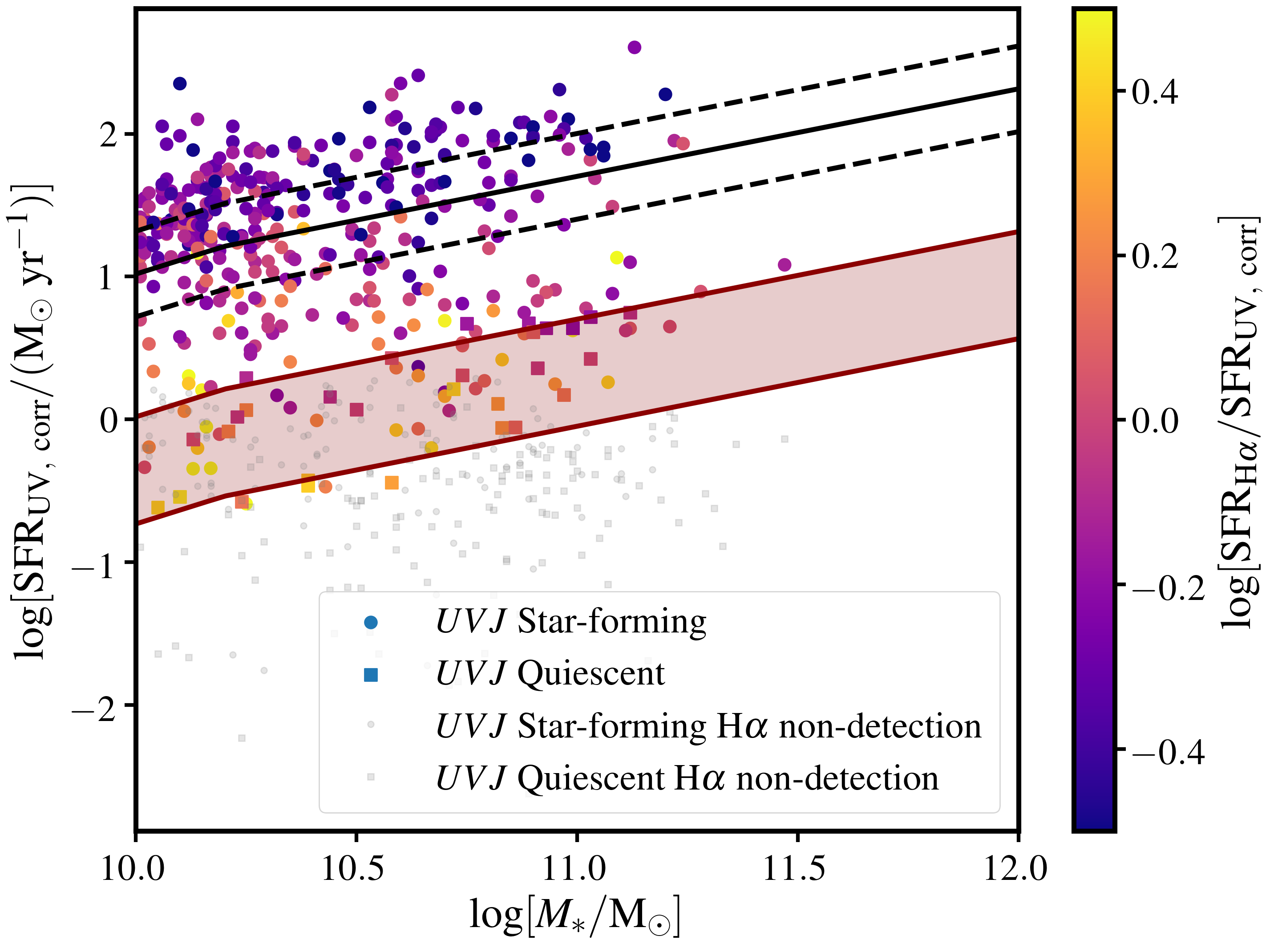
Figure 1 illustrates this sample in the diagram, as well as a diagram showing the sample in vs. dereddened space. The observed colors are dereddened using a Calzetti et al. 2000 extinction law and extinction from the best-fit SED in the CANDELS catalogs (see Sec. 2.1). Figure 2 shows the sample in SFR- space. In both figures, points are color-coded by the ratio between and UV SFRs for objects with emission. It is already clear that, while most objects with emission are classified as star-forming, of -quiescent objects and of objects more than dex below the main sequence have significant emission. To specifically investigate the nature of the SFH of galaxies in the process of quenching, we narrow our focus further to the systems ( of which are -star forming and of which are -quiescent) whose dust-correct UV SFRs are between and dex below the main sequence of Whitaker et al. 2014 in our modeling (Section 3). This space is highlighted in Figure 2.
2.1 SFR measurements
The UV-based SFR, which is sensitive to stars less than Myr old, is derived from the UV luminosity at Å following the Wuyts et al. 2011 conversion:
| (1) |
where SFRUV is the dust-corrected UV SFR in units of and is the luminosity at Å in units of taken from the best-fit SED. We assume a Calzetti et al. 2000 extinction law, such that , where is the -band reddening. Because low-SFR galaxies (at least dex below the main sequence) in our analysis have relatively little dust (), the adoption of an alternative extinction law has a negligible effect on our results. For example, adopting an SMC law (Gordon et al. 2003) alters the UV SFRs by dex and the ratio between UV and SFRs by dex for of low-SFR objects. Deep imaging from , the CFHT, and Subaru telescope sample this region of the SED to a depth of approximately , resulting in an unobscured SFR limit of at .
At high redshifts, a majority of the UV light from star-formation is absorbed and re-emitted in the far-IR (Whitaker et al. 2014). While far-IR measurements from or ground-based sub-mm telescopes can measure this directly for a limited number of bright objects, most survey-based studies rely on a luminosity-dependent conversion from µm flux to a total IR luminosity (Whitaker et al. 2014; Whitaker et al. 2017). However, diffuse dust heated from old stars, in addition to emission directly from asymptotic-giant branch (AGB) stars, can contribute substantially to the observed m flux for galaxies with low SFRs (Piovan et al. 2003; Marigo et al. 2008; Kelson & Holden 2010; Fumagalli et al. 2014). Additionally the conversion between polycyclic aromatic hydrocarbon (PAH) emission (the origin of µm emission at high ) and SFR depends on the age and ionizing flux of the stellar population (Shivaei et al. 2017), which may vary significantly across our sample.

Given these uncertainties, we elect to use the UV luminosity corrected for extinction, which primarily derives from young stars, to measure the star-formation activity on these timescales. By comparing our dust-corrected UV SFRs with Herschel-based SFRs available for a subset of our sample ( objects, of which have dust-corrected UV SFRs greater than ), we have determined that using the extinction reported in the 3D-HST catalogs results in a correlation between extinction and the ratio of Herschel-based SFRs-to-dust-corrected UV SFRs, even among galaxies for which Herschel observations are complete. Alternatively, using the median reported in the CANDELS catalogs, combining different SED fits with different assumptions (Nayyeri et al. 2017; Stefanon et al. 2017; Guo et al. 2013; Galametz et al. 2013), results in agreement between the UV-corrected SFRs and UV+IR SFRs within and independent of the amount of extinction for objects with UV-corrected SFRs greater than (see Fig. 3). Moreover, Balmer-decrement-based extinction measurements for objects in the LEGA-C survey (van der Wel et al. 2016) agree with the CANDELS extinction measurement better than the 3D-HST measurement. The UV-corrected SFRs agree with the SFR of the best-fit SED for star-forming objects, further suggesting that the dust-corrected UV SFRs are accurate. For objects with low SFRs, the above recipe may overestimate their true SFRs because emission from Post-AGB stars, Blue-Horizontal-Branch Stars, and Blue Stragglers can represent a non-negligible fraction of the UV luminosity (Dorman et al. 1995). Because this emission depends on the SFH of the galaxy in a non-trivial way, we incorporate it into our modeling (see Sec. 3 and 5.1.2) rather than subtracting this emission when calculating the UV SFR.
The -based SFRs (SFRHα) are calculated from the Kennicutt & Evans 2012 conversion adjusted to a Chabrier IMF following Muzzin et al. 2010:
| (2) |
where is the luminosity of the line in solar luminosities, and AHα is the internal extinction of the line. The H flux limit achieved by 3D-HST of erg/s/cm2 corresponds to a H SFR of at assuming . To accurately measure SFRs, we correct the luminosity for (1) extinction, (2) stellar absorption, (3) emission from post-AGB stars, and (4) contamination from nearby [Nii] emission (in that order).
The SFRs are corrected for extinction following a Calzetti et al. 2000 law. Following Wuyts et al. 2013, we relate the nebular extinction to the continuum emission as , where is the continuum extinction at . For a subsample () of objects with H detections from the LEGA-C survey (van der Wel et al. 2016), the Balmer-decrement-based extinction measurements are generally consistent with the extinction determined from the continuum extinction, with an median deviation of mag and dispersion of mag. Among these objects, there is no correlation between the deviation and the measured extinction.
We correct for absorption, which can be significant for massive galaxies (Kauffmann et al. 2003), using an age-dependent factor based on the amount of absorption in spectra generated following the model SFHs used in our analysis (see Sec. 3). On average, for our star-formation histories, this varies with age according to:
| (3) |
where EW is the is the equivalent width of absorption and is the bolometric light-weighted age of the stellar population in Gyr. For each galaxy, the light-weighted age from the the 3D-HST catalog is used in conjunction with Equation 3 to determine the amount of absorption. However, if a constant absorption of Å is adopted, the change in our results is negligible. For star-forming galaxies, this correction lowers the sSFR by yr-1; for older quiescent galaxies, it corresponds to a decrease of yr-1.
Furthermore, post-AGB stars can produce enough ionizing radiation to contribute significantly to the luminosity (Cid Fernandes et al. 2011; Singh et al. 2013; Belfiore et al. 2016). Although there remains uncertainty with regard to the specifics of AGB and post-AGB stellar evolution, models generally agree that evolved stars provide an ionizing flux of photonss (Cid Fernandes et al. 2011) independent of age. Assuming Case-B recombination and a temperature of K, this corresponds to a luminosity per stellar mass of erg s-1 -1. Given that evolved stellar-populations have [Nii]/ ratios close to (Belfiore et al. 2016), we subtract erg s-1 (corresponding to a sSFR of yr-1) from the luminosity to isolate the emission associated with young stars.
Because of the low spectral resolution of the grism, the measured flux contains emission from both and nearby [Nii]. To correct for this contamination, we adopt a mass-dependent correction motivated by the mass-metallicity relation. The gas-phase metallicity is estimated from the measured stellar mass assuming the redshift-dependent mass-metallicity relation of Zahid et al. 2014, and the metallicity is converted to a [Nii]/ flux ratio following Kewley & Ellison 2008. The flux reported in the 3D-HST catalog is reduced by this ratio to determine the flux. This physically-motivated correction (typically around for our sample) is somewhat larger than the usually assumed (Wuyts et al. 2011).
3 Results
Figure 4 shows the ratio between and UV SFR measurements (which we refer to as as a function of the offset between the UV SFR and the Whitaker et al. 2014 main sequence MS, color coded by their location in space (Wuyts et al. 2007; Williams et al. 2009) using the Whitaker et al. 2012 definition. As expected, both SFR measures agree for galaxies with ongoing star formation. As galaxies drop below the main sequence, more systems have low or undetected emission as the instantaneous SFR (traced by ) decreases more quickly than the average SFR (traced by UV). However, there remains a significant population of systems with close to . Notably, of -quiescent objects and of objects more than dex below the main sequence have significant emission.
While -quiescent objects with emission have higher values than -quiescent objects on average, most are characterized by , suggesting that they are generally not dusty contaminants. Significant m emission is present in only of -quiescent objects and of objects more than dex below the main sequence. Although there remains uncertainty regarding the amount of m emission that originates from old stars, the m luminosities of objects with m emission can generally be accounted for with a combination of low level star formation (consistent with their dust-corrected UV SFRs) and emission from an old stellar population (Leroy et al. 2012; Salim et al. 2007; Kelson & Holden 2010). Altogether, although dusty contaminants may be present in our sample, they likely don’t represent a significant source of contamination for our study.
Galaxies on the main sequence are consistent with and have a small ( dex) scatter in , but the distribution of fluxes and non-detections among galaxies below the main sequence implies evolution of as systems fall off of the main sequence. Assuming is normally distributed, the mean and standard deviation of that distribution that best-fit the distribution of fluxes and non-detections among low-SFR galaxies is and dex respectively.
To address the possibility that this emission is from bursty star formation, we illustrate how evolves as a function of MS for various model star-formation histories (SFHs).

All models are based on an exponentially declining plus exponential burst star-formation history following a period of constant SFR of the form:
| (4) |
where SFR0 is the SFR of the galaxy before quenching occurs, is the time when the galaxy quenches, is the quenching timescale, is the peak burst amplitude, corresponds to when the burst occurs after the initial quenching, and is the characteristic timescale of the burst. First, we consider two bursty models with Myr and : models A and B have Gyr and Gyr respectively. Although is not constrained in general, our choice of Myr is motivated by studies of recently quenched galaxies finding stellar ages consistent with short timescales (Zick et al. 2018; French et al. 2018; Belli et al. 2019). Additionally, we consider two no-burst models to compare with our bursty models. Model C is a smooth model with Myr and closely resembles model A in most other aspects. Model D, which is characterized by Gyr, represents the null hypothesis of quenching too slow to alter the /UV SFR ratio (models with longer than the Myr lifetime of a B star quickly resemble the Gyr model). These models are summarized in Table 1. For each SFH, we model the stellar population using the pyfsps code (Conroy et al. 2009; Conroy & Gunn 2010; Foreman-Mackey et al. 2014). We initialize all models with Gyr of continuous star formation at (mimicking the formation of a galaxy to match the initial colors and UV luminosities), after which point, SFR follows Equation 4. The models all have a solar metallicity and a Chabrier IMF. The adoption of a higher metallicty could change the inferred UV SFR, but the distribution of systems with is statistically identical to the distribution of systems with among transition population (systems dex below the main sequence). This evidence, combined with the fact that stellar metallicity is observed to vary by less than dex across our the mass range of our sample for low-SFR galaxies (Choi et al. 2014; Estrada-Carpenter et al. 2019), suggests that the adoption of a uniform solar metallicity for our models is not unrealistic. From the synthesized spectra, the UV and SFRs are calculated according to equations 1 and 2, respectively. These models are not meant to span the entire range of plausible scenarios; rather they give a general sampling of what different quenching models predict.
These star-formation histories are summarized in Figure 5. As seen in Figure 4, decreases dramatically with increasing MS for all models with Myr. For Gyr, remains roughly constant during the quenching process. The bursty models are distinguished by a sharp increase in during the burst due to emission from young stars. In particular, bursty SFHs predict a large range of for low SFRs present in the data, while smooth SFHs predict a narrow range of values at a given UV SFR.
| Model | () | (Gyr) | (Myr) | (Myr) |
|---|---|---|---|---|
| A | 1 | 0.3 | 100 | 100 |
| B | 1 | 1.25 | 100 | 100 |
| C | 0 | – | 200 | – |
| D | 0 | – | 1000 | – |
4 Modeling the Transition Population
To test which SFH model best matches the observations, we model the expected flux distribution among galaxies between and dex below the main sequence.

For each model SFH described above, we construct an expected flux distribution based on the objects in our sample. Specifically, we determine the expected flux for each object given its UV SFR and the value predicted by each particular SFH as follows:
- 1.
For each galaxy in our sample, the initial SFR (SFR0) is taken to be the SFR of a galaxy with the same stellar mass and redshift on the Whitaker et al. 2014 main sequence plus normally-distributed scatter of dex.
- 2.
The value of is estimated from the assumed SFH and the observed UV SFR. The ratio between the observed UV SFR and SFR0 is taken to be SFR/SFR0 in equation 4 and used to determine , which is in turn used to determine (see Fig. 5). In the case that this results in multiple values of , the dereddened diagonal color (, from Fang et al. 2018) of the galaxy is compared with the model at the various times. The time with the closest color to the observed galaxy is used. The SFR is determined from the value and the dust-corrected UV SFR.
- 3.
The SFR is converted to an luminosity.
- 4.
Absorption at is subtracted from the luminosity following Equation 3 using the bolometric light-weighted age as .
- 5.
Emission from AGB stars is added to the luminosity as erg s-1 -1 times the observed stellar mass (the factor of accounts for [Nii] emission from AGB stars, which is characterized by an [Nii]/ ratio of ).
- 6.
The luminosity is corrected for attenuation and [Nii] contamination with the same prescriptions as described in Section 2.
- 7.
This luminosity is converted to flux, and a normally-distributed error of erg/s/cm2 is added to this measurement (Momcheva et al. 2016).
Although X-ray-detected AGN are excluded from our sample, we include the effects of any X-ray-non-detected AGN in our model. Using the mass and redshift-dependent AGN luminosity functions of Aird et al. 2012, we predict the fraction of our subsample expected to host AGN. We take the difference between the expected AGN occurrence and the number of observed AGN as the number of X-ray-non-detected AGN. This number of galaxies is randomly selected from our sample, and for each supposed non-detected AGN, we replace the luminosity expected from the SFH model with the luminosity expected given the /UV ratio of a randomly chosen X-ray-detected AGN. Undetected AGN represent of our subsample and their /UV ratios are not substantially different than the non-AGN population, so this correction does not have a substantial impact on the analysis. Additionally, excluding AGN based on their IRAC colors, which is more sensitive to extremely dust-extincted AGN compared with X-ray-AGN (Stern et al. 2005), does not affect our conclusions.
Figure 6 illustrates the distributions of +[Nii] flux for both the observations (solid histogram) and the models (hatched histograms) for galaxies between and dex below the main sequence. Also shown are the results of an Anderson Darling test comparing the predicted distributions with observations. For this test, all objects with flux less than erg s-1 cm-2 are considered non-detections and considered to have flux. The slow quenching model (model D) substantially overpredicts the number of detections. On the other hand, while the faster smooth model (model C) only slightly underpredicts the number of detections, it significantly underpredicts the observed flux for these objects. The quick burst of model A means that by the time the UV SFR is below the main sequence, values quickly and unformly fall, such that it underpredicts the flux throughout this sample. The large degree of variation in in model B, however, is able to reproduce the large variation in fluxes apparent in our sample.

4.1 Rest-Frame Colors
As an independent test of the SFHs of galaxies, we compare the values with rest-frame, de-reddened colors in Figure 7. Again, we find that blue star-forming galaxies have values close to , whereas red quiescent galaxies have a wide range of values. In Figure 8, we show the distributions produced through the same method as Figure 6, but with color in place of UV SFR. For objects with , where of objects more than dex below the main sequence live, the distribution is again most consistent with bursty model B.


5 Discussion
In this analysis, we find that a bursty SFH is required in order to reproduce the large range in the /UV ratios of galaxies with low SFRs. In this section we discuss a few possible origins of this result. First, we discuss the effect of various systematics related to measuring/interpreting the and UV SFRs of galaxies in our sample. Next, we discuss possible physical mechanisms driving the range of values observed in our sample.
5.1 Systematics
5.1.1 Emission from Active Galactic Nuclei
While we account for X-ray AGN in our analysis, it is possible that low-luminosity or obscured AGN contribute to the emission of these sources. Indeed Belli et al. 2017 have found that a number of -quiescent objects with emission have [Nii]/ ratios consistent with an AGN. However, for a wide range of UV luminosities, the inferred and UV SFRs are in agreement (see Fig. 4), so there is no reason to believe that low-level AGN present a significant bias in our modeling. Additionally, X-ray non-detected AGN are not expected to represent a substantial fraction of our sample, further suggesting that the presence of an AGN does not significantly affect our conclusions.
5.1.2 Emission from Evolved Stars
UV emission from evolved stars is apparent in local elliptical galaxies (Dorman et al. 1995). Studies of the spectra and colors of these galaxies suggest that this emission is primarily due to post-AGB and Blue-Horizontal-Branch stars (Yan 2018). This emission is nominally included in the pyfsps models, but significant uncertainties remain in our understanding of this phase of stellar-evolution, so our models may be underestimating the UV luminosity of evolved stellar populations. However, this uncertainty does not affect our conclusions: if evolved stars contribute more UV emission than our models, our models should move down and to the right in Figure 4 except for during a burst, during which UV emission is dominated by young stars and the contribution from evolved stars is negligible. In this case, smooth models would be a worse fit to the distribution, whereas bursty models would better fit the distribution.
5.1.3 Extra Extinction Around Hii Regions
A significant source of uncertainty regarding this analysis is the amount of extra extinction around Hii regions. Because the relationship between stellar and nebular extinction solely affects the SFR, adjusting this ratio would directly alter our results. However, while this relationship is important to ensure that both SFR measures agree for star-forming galaxies, the median extinction value for quiescent objects is only , so extinction does not play a very important role in calculating the SFRs of the low-SFR population. If we adopt the slightly higher nebular-to-continuum extinction ratio (known as the factor) from Calzetti et al. 2000, model C fits the observations slightly better, but our model B remains the best fitting model. Adopting a lower nebular-to-continuum ratio, as suggested by some recent high- studies (Puglisi et al. 2016; Broussard et al. 2019, for ex. ), improves the fit of model A and weakens the fit of model B. However, using a lower ratio overestimates for systems on the star-forming main sequence: adopting an factor of changes the median value among objects within dex of the main sequence from to . The suggested variation in factor at higher redshift is driven by dusty objects with high SFRs (Reddy et al. 2015), whereas our sample has sSFRs more similar to low- objects. Observations of local galaxies suggest that low-sSFR galaxies that have Calzetti-like factors, whereas high sSFR galaxies (like those at high ) have lower factors (Battisti et al. 2016). Additionally, the agreement between Balmer-decrement-based measurements and our measurements, as well as the fact that is not correlated with extinction among our sample, suggests that this is not a significant issue (see Fig. 3).
5.1.4 Contamination from [Nii]
Contamination from nearby [Nii] represents a non-negligible contribution to the observed flux (and inferred values). If the [Nii]/ ratio is substantially higher among our sample, the inferred values could be overestimated. Indeed, [Nii] emission from high- galaxies appears higher than expected given their [OIII]/H ratios (Steidel et al. 2014; Masters et al. 2014; Jones et al. 2015; Shapley et al. 2015, but see Sanders et al. 2018). Increasing the [Nii]/ ratio by dex increases the predicted flux distribution, bringing models A and C in better agreement with observations. The [Nii] offset appears to be constant with SFR (Strom et al. 2017), which would induce a roughly constant shift in for all SFRs, not a preferentially lower for low-SFR galaxies in particular, as would be necessary for our measurements to match a smoothly declining SFH. Furthermore, there is no residual trend between and stellar mass, as one would expect if this metallicity-dependent effect was important.
5.2 Physical Mechanisms
5.2.1 Initial Mass Function
As emission primarily is dominated by stars with , whereas UV emission originates from stars with , the ratio of the two SFR measures is sensitive to the intial mass function (IMF) of the stellar population. In particular, Fumagalli et al. 2011 and da Silva et al. 2014 have suggested that stochastic sampling of the initial mass function, both due to limited mass and time resolution at low SFRs may be responsible for variation in /UV SFRs. To test the impact of stochastic IMF sampling on our model, we utilize the slug code (Krumholz et al. 2015). Contrary to traditional stellar-population synthesis codes which integrate a given IMF to a certain mass regardless of the overall SFR, this code directly and stochastically samples the IMF to generate stellar populations. However, the dispersion in the to UV ratio for a model with an SFR of (corresponding to MS) is only dex (with the fraction of stars formed in clusters set to ), not enough to explain the large dispersion in values.
Alternatively, a very top-heavy IMF could result in systematically higher values compared with the Chabrier values. We test this hypothesis using the van Dokkum 2008 parameterization of the IMF, with set to (at the high end of what is observed). In this case, UV and emission decrease at similar rates, even for the fast quenching models, such that no model is able to reproduce the large number of galaxies with low values. The primary effect of adopting a more-bottom heavy IMF (as suggested by some observations of nearby massive ellipticals van Dokkum et al. 2017) is a decrease in UV and emission at a given SFR. Still, the large dispersion in SFRs for galaxies with low UV SFRs cannot be reproduced by any smooth quenching model and is best reproduced by model B. Similarly, an integrated galactic-IMF (IGIMF), in which stars are formed primarily in clusters (Weidner & Kroupa 2005; Weidner et al. 2011), results in more top-heavy for galaxies with lower SFRs. Following Pflamm-Altenburg et al. 2007, we adjust the -to-SFR ratio for their Minimal-1 and Standard models. However, for both models, the variation of the luminosity with SFR is not sufficient to explain the observed variation and no SFH model matches the observed distribution with a value higher than .
5.2.2 Minor Mergers
Within massive galaxies, bursty star formation is often though of as due to minor mergers or interactions (Mihos & Hernquist 1994; Somerville et al. 2008). For galaxies at , the major merger rate is Mpc-3 Gyr-1 (Duncan et al. 2019), corresponding to per galaxy per Gyr. Assuming that minor merger rate is a factor of higher than the major merger rate (Rodriguez-Gomez et al. 2015), we would minor mergers to be common among our sample. This suggests that minor mergers driving bursty star formation could explain the observed burstiness in our population.
6 Conclusions
Using data from the 3D-HST survey, we analyze emission within massive galaxies at , focusing on galaxies undergoing the transition between star-forming and quiescence to better understand the process of quenching in these galaxies. Our conclusions are as follows.
- •
In contrast with expectations, we find evidence of emission for galaxies down to the lowest levels of UV SFR present in our sample, including of systems identified as quiescent through the diagram.
- •
There is a large dispersion ( dex) in the ratio between and UV SFRs for galaxies with low UV SFRs. Even after accounting for the expected emission from AGN and evolved stars, this large range is inconsistent with a smoothly declining star-formation history.
- •
The observed variation in -to-UV SFRs among massive galaxies in the process of quenching implies that quenching at is not characterized by a continuous decline in SFR. On the contrary, by modeling various bursty and non-bursty star-formation histories, we show that, bursty star formation continues as the SFR declines.
Our analysis has been limited to high-mass systems due to the limited S/N of lower mass systems, but given that they have bursty star formation when they are star forming, an analysis of the emission in low-mass galaxies transitioning to quiescence would be particularly valuable.
Acknowledgments
We are grateful to the anonymous reviewer, whose suggestions greatly improved this paper. This research made use of Astropy, a community-developed core Python package for Astronomy (Astropy Collaboration et al. 2013). Additionally, the Python packages NumPy (Walt et al. 2011), iPython (Pérez & Granger 2007), SciPy (Jones et al. 2001), and matplotlib (Hunter 2007) were utilized for the majority of our data analysis and presentation.
Appendix A Other Star-formation Histories
While it is beyond the scope of this work to evaluate all possible bursty SFHs, we explore the effects of varying the burst timescale, delay time, and strength in this appendix. In Table 2, we describe SFHs that we explore beyond the described in our primary analysis in the form of
| (5) |
with representing the burst amplitude, representing the time of quenching, representing the burst delay time, and representing the exponential timescale of the burst.
Figure 9 shows the relationship between and MS for these SFHs in comparison with our observations. The most important variable is the burst delay time: models with high values are able to reach lower SFR values before bursting. As shown in Figure 10, bursty model F is preferred to any smoothly declining model.
We also consider linearly increasing, delayed, and inverted tau models in the form of:
| (6) |
| (7) |
and
| (8) |
with SFR0, , , , and values as in models A, B, C, and D. The parameters describing these models as well as the results of our comparison of these models with observations are found in Table 2. For the delayed model (equation 7), no model accurately reproduces the flux distribution for objects between and dex below the main sequence. For the inverse model (equation 8), bursty model B reproduces the flux distribution, whereas smooth model C does not. Lastly, for the linearly increasing model (equation 6), both model B and C reproduce the observed flux distribution for objects between and dex below the main sequence. Model B fits the distribution for objects with dust-corrected colors between and and model C does not, however. In summary, regardless of the general form of the star-formation history adopted in our models, a bursty star-formation history better fits the observed fluxes compared with a smoothly-declining star-formation history.

| Model | SFH Equation | () | (Gyr) | (Myr) | (Myr) | value (MS) | value (dereddened ) |
|---|---|---|---|---|---|---|---|
| E | 4 | 0 | – | 100 | – | ||
| F | 4 | 3 | 1 | 100 | 100 | ||
| G | 4 | 1 | 1 | 200 | 200 | ||
| H | 4 | 3 | 1 | 200 | 200 | ||
| A Increasing | 6 | 1 | 0.3 | 100 | 100 | ||
| B Increasing | 6 | 1 | 1.25 | 100 | 100 | ||
| C Increasing | 6 | 0 | – | 200 | – | ||
| D Increasing | 6 | 0 | – | 1000 | – | ||
| A Delayed | 7 | 1 | 0.3 | 100 | 100 | ||
| B Delayed | 7 | 1 | 1.25 | 100 | 100 | ||
| C Delayed | 7 | 0 | – | 200 | – | ||
| D Delayed | 7 | 0 | – | 1000 | – | ||
| A Inverse | 8 | 1 | 0.3 | 100 | 100 | ||
| B Inverse | 8 | 1 | 1.25 | 100 | 100 | ||
| C Inverse | 8 | 0 | – | 200 | – | ||
| D Inverse | 8 | 0 | – | 1000 | – |

References
- Aird et al. (2012) Aird J., et al., 2012, ApJ, 746, 90
- Astropy Collaboration et al. (2013) Astropy Collaboration et al., 2013, A&A, 558, A33
- Balogh et al. (2004) Balogh M. L., Baldry I. K., Nichol R., Miller C., Bower R., Glazebrook K., 2004, ApJ, 615, L101
- Battisti et al. (2016) Battisti A. J., Calzetti D., Chary R. R., 2016, ApJ, 818, 13
- Beckmann et al. (2017) Beckmann R. S., et al., 2017, MNRAS, 472, 949
- Belfiore et al. (2016) Belfiore F., et al., 2016, MNRAS, 461, 3111
- Bell et al. (2004) Bell E. F., et al., 2004, ApJ, 608, 752
- Belli et al. (2017) Belli S., et al., 2017, ApJ, 841, L6
- Belli et al. (2019) Belli S., Newman A. B., Ellis R. S., 2019, ApJ, 874, 17
- Brammer et al. (2008) Brammer G. B., van Dokkum P. G., Coppi P., 2008, ApJ, 686, 1503
- Broussard et al. (2019) Broussard A., et al., 2019, ApJ, 873, 74
- Calzetti et al. (2000) Calzetti D., Armus L., Bohlin R. C., Kinney A. L., Koornneef J., Storchi-Bergmann T., 2000, ApJ, 533, 682
- Carnall et al. (2018) Carnall A. C., McLure R. J., Dunlop J. S., Davé R., 2018, MNRAS, 480, 4379
- Ceverino & Klypin (2009) Ceverino D., Klypin A., 2009, ApJ, 695, 292
- Chabrier (2003) Chabrier G., 2003, PASP, 115, 763
- Choi et al. (2014) Choi J., Conroy C., Moustakas J., Graves G. J., Holden B. P., Brodwin M., Brown M. J. I., van Dokkum P. G., 2014, ApJ, 792, 95
- Cid Fernandes et al. (2011) Cid Fernandes R., Stasińska G., Mateus A., Vale Asari N., 2011, MNRAS, 413, 1687
- Conroy & Gunn (2010) Conroy C., Gunn J. E., 2010, ApJ, 712, 833
- Conroy et al. (2009) Conroy C., Gunn J. E., White M., 2009, ApJ, 699, 486
- Croton et al. (2006) Croton D. J., et al., 2006, MNRAS, 365, 11
- Daddi et al. (2005) Daddi E., et al., 2005, ApJ, 626, 680
- Dekel & Birnboim (2006) Dekel A., Birnboim Y., 2006, MNRAS, 368, 2
- Di Matteo et al. (2005) Di Matteo T., Springel V., Hernquist L., 2005, Nature, 433, 604
- Dorman et al. (1995) Dorman B., O’Connell R. W., Rood R. T., 1995, ApJ, 442, 105
- Duncan et al. (2019) Duncan K., et al., 2019, ApJ, 876, 110
- Estrada-Carpenter et al. (2019) Estrada-Carpenter V., et al., 2019, ApJ, 870, 133
- Faber et al. (2007) Faber S. M., et al., 2007, ApJ, 665, 265
- Fang et al. (2018) Fang J. J., et al., 2018, ApJ, 858, 100
- Foreman-Mackey et al. (2014) Foreman-Mackey D., Sick J., Johnson B., 2014, python-fsps: Python bindings to FSPS (v0.1.1), doi:10.5281/zenodo.12157, https://doi.org/10.5281/zenodo.12157
- French et al. (2018) French K. D., Yang Y., Zabludoff A. I., Tremonti C. A., 2018, ApJ, 862, 2
- Fumagalli et al. (2011) Fumagalli M., da Silva R. L., Krumholz M. R., 2011, ApJ, 741, L26
- Fumagalli et al. (2014) Fumagalli M., et al., 2014, ApJ, 796, 35
- Galametz et al. (2013) Galametz A., et al., 2013, ApJS, 206, 10
- Goddard et al. (2017) Goddard D., et al., 2017, MNRAS, 466, 4731
- Gordon et al. (2003) Gordon K. D., Clayton G. C., Misselt K. A., Land olt A. U., Wolff M. J., 2003, ApJ, 594, 279
- Grogin et al. (2011) Grogin N. A., et al., 2011, ApJS, 197, 35
- Guo et al. (2013) Guo Y., et al., 2013, ApJS, 207, 24
- Guo et al. (2016) Guo Y., et al., 2016, ApJ, 833, 37
- Hahn et al. (2017) Hahn C., Tinker J. L., Wetzel A., 2017, ApJ, 841, 6
- Hopkins et al. (2006) Hopkins P. F., Hernquist L., Cox T. J., Di Matteo T., Robertson B., Springel V., 2006, ApJS, 163, 1
- Hopkins et al. (2014) Hopkins P. F., Kereš D., Oñorbe J., Faucher-Giguère C.-A., Quataert E., Murray N., Bullock J. S., 2014, MNRAS, 445, 581
- Hunter (2007) Hunter J. D., 2007, Computing in Science & Engineering, 9, 90
- Ilbert et al. (2013) Ilbert O., et al., 2013, A&A, 556, A55
- Jones et al. (2001) Jones E., Oliphan T., Peterson P., et al., 2001, SciPy: Open source scientific tools for Python, http://www.scipy.org/
- Jones et al. (2015) Jones T., Martin C., Cooper M. C., 2015, ApJ, 813, 126
- Kauffmann et al. (2003) Kauffmann G., et al., 2003, MNRAS, 341, 33
- Kelson & Holden (2010) Kelson D. D., Holden B. P., 2010, ApJ, 713, L28
- Kennicutt & Evans (2012) Kennicutt R. C., Evans N. J., 2012, ARA&A, 50, 531
- Kereš et al. (2005) Kereš D., Katz N., Weinberg D. H., Davé R., 2005, MNRAS, 363, 2
- Kewley & Ellison (2008) Kewley L. J., Ellison S. L., 2008, ApJ, 681, 1183
- Koekemoer et al. (2011) Koekemoer A. M., et al., 2011, ApJS, 197, 36
- Kriek et al. (2009) Kriek M., van Dokkum P. G., Labbé I., Franx M., Illingworth G. D., Marchesini D., Quadri R. F., 2009, ApJ, 700, 221
- Krumholz et al. (2015) Krumholz M. R., Fumagalli M., da Silva R. L., Rendahl T., Parra J., 2015, MNRAS, 452, 1447
- Kuntschner et al. (2010) Kuntschner H., et al., 2010, MNRAS, 408, 97
- Leroy et al. (2012) Leroy A. K., et al., 2012, AJ, 144, 3
- Marigo et al. (2008) Marigo P., Girardi L., Bressan A., Groenewegen M. A. T., Silva L., Granato G. L., 2008, A&A, 482, 883
- Martig et al. (2009) Martig M., Bournaud F., Teyssier R., Dekel A., 2009, ApJ, 707, 250
- Martin et al. (2007) Martin D. C., et al., 2007, ApJS, 173, 342
- Masters et al. (2014) Masters D., et al., 2014, ApJ, 785, 153
- Mihos & Hernquist (1994) Mihos J. C., Hernquist L., 1994, ApJ, 425, L13
- Momcheva et al. (2016) Momcheva I. G., et al., 2016, ApJS, 225, 27
- Muzzin et al. (2010) Muzzin A., van Dokkum P., Kriek M., Labbé I., Cury I., Marchesini D., Franx M., 2010, ApJ, 725, 742
- Nandra et al. (2015) Nandra K., et al., 2015, ApJS, 220, 10
- Nayyeri et al. (2017) Nayyeri H., et al., 2017, ApJS, 228, 7
- Oppenheimer & Davé (2006) Oppenheimer B. D., Davé R., 2006, MNRAS, 373, 1265
- Pandya et al. (2017) Pandya V., et al., 2017, MNRAS, 472, 2054
- Peng et al. (2010) Peng Y.-j., et al., 2010, ApJ, 721, 193
- Pflamm-Altenburg et al. (2007) Pflamm-Altenburg J., Weidner C., Kroupa P., 2007, ApJ, 671, 1550
- Piovan et al. (2003) Piovan L., Tantalo R., Chiosi C., 2003, A&A, 408, 559
- Puglisi et al. (2016) Puglisi A., et al., 2016, A&A, 586, A83
- Pérez & Granger (2007) Pérez F., Granger B. E., 2007, Computing in Science & Engineering, 9, 21
- Rangel et al. (2013) Rangel C., Nandra K., Laird E. S., Orange P., 2013, MNRAS, 428, 3089
- Reddy et al. (2010) Reddy N. A., Erb D. K., Pettini M., Steidel C. C., Shapley A. E., 2010, ApJ, 712, 1070
- Reddy et al. (2015) Reddy N. A., et al., 2015, ApJ, 806, 259
- Rodriguez-Gomez et al. (2015) Rodriguez-Gomez V., et al., 2015, MNRAS, 449, 49
- Salim et al. (2007) Salim S., et al., 2007, ApJS, 173, 267
- Salim et al. (2009) Salim S., et al., 2009, ApJ, 700, 161
- Salvato et al. (2011) Salvato M., et al., 2011, ApJ, 742, 61
- Sanders et al. (2018) Sanders R. L., et al., 2018, ApJ, 858, 99
- Schawinski et al. (2007) Schawinski K., Thomas D., Sarzi M., Maraston C., Kaviraj S., Joo S.-J., Yi S. K., Silk J., 2007, MNRAS, 382, 1415
- Schawinski et al. (2014) Schawinski K., et al., 2014, MNRAS, 440, 889
- Shapley et al. (2015) Shapley A. E., et al., 2015, ApJ, 801, 88
- Shivaei et al. (2015) Shivaei I., Reddy N. A., Steidel C. C., Shapley A. E., 2015, ApJ, 804, 149
- Shivaei et al. (2017) Shivaei I., et al., 2017, ApJ, 837, 157
- Singh et al. (2013) Singh R., et al., 2013, A&A, 558, A43
- Skelton et al. (2014) Skelton R. E., et al., 2014, ApJS, 214, 24
- Somerville et al. (2008) Somerville R. S., Hopkins P. F., Cox T. J., Robertson B. E., Hernquist L., 2008, MNRAS, 391, 481
- Sparre et al. (2017) Sparre M., Hayward C. C., Feldmann R., Faucher-Giguère C.-A., Muratov A. L., Kereš D., Hopkins P. F., 2017, MNRAS, 466, 88
- Stefanon et al. (2017) Stefanon M., et al., 2017, ApJS, 229, 32
- Steidel et al. (2014) Steidel C. C., et al., 2014, ApJ, 795, 165
- Stern et al. (2005) Stern D., et al., 2005, ApJ, 631, 163
- Strom et al. (2017) Strom A. L., Steidel C. C., Rudie G. C., Trainor R. F., Pettini M., Reddy N. A., 2017, ApJ, 836, 164
- Thomas et al. (2010) Thomas D., Maraston C., Schawinski K., Sarzi M., Silk J., 2010, MNRAS, 404, 1775
- Ueda et al. (2008) Ueda Y., et al., 2008, ApJS, 179, 124
- Walt et al. (2011) Walt S. v. d., Colbert S. C., Varoquaux G., 2011, Computing in Science & Engineering, 13, 22
- Weidner & Kroupa (2005) Weidner C., Kroupa P., 2005, ApJ, 625, 754
- Weidner et al. (2011) Weidner C., Kroupa P., Pflamm-Altenburg J., 2011, MNRAS, 412, 979
- Weisz et al. (2012) Weisz D. R., et al., 2012, ApJ, 744, 44
- Wetzel et al. (2013) Wetzel A. R., Tinker J. L., Conroy C., van den Bosch F. C., 2013, MNRAS, 432, 336
- Whitaker et al. (2012) Whitaker K. E., van Dokkum P. G., Brammer G., Franx M., 2012, ApJ, 754, L29
- Whitaker et al. (2014) Whitaker K. E., et al., 2014, ApJ, 795, 104
- Whitaker et al. (2017) Whitaker K. E., et al., 2017, ApJ, 838, 19
- Wild et al. (2016) Wild V., Almaini O., Dunlop J., Simpson C., Rowlands K., Bowler R., Maltby D., McLure R., 2016, MNRAS, 463, 832
- Williams et al. (2009) Williams R. J., Quadri R. F., Franx M., van Dokkum P., Labbé I., 2009, ApJ, 691, 1879
- Wisnioski et al. (2019) Wisnioski E., et al., 2019, arXiv e-prints, p. arXiv:1909.11096
- Worthey & Ottaviani (1997) Worthey G., Ottaviani D. L., 1997, ApJS, 111, 377
- Wuyts et al. (2007) Wuyts S., et al., 2007, ApJ, 655, 51
- Wuyts et al. (2011) Wuyts S., et al., 2011, ApJ, 738, 106
- Wuyts et al. (2013) Wuyts S., et al., 2013, ApJ, 779, 135
- Xue et al. (2011) Xue Y. Q., et al., 2011, ApJS, 195, 10
- Yan (2018) Yan R., 2018, MNRAS, 481, 476
- Zahid et al. (2014) Zahid H. J., Dima G. I., Kudritzki R.-P., Kewley L. J., Geller M. J., Hwang H. S., Silverman J. D., Kashino D., 2014, ApJ, 791, 130
- Zick et al. (2018) Zick T. O., et al., 2018, ApJ, 867, L16
- da Silva et al. (2014) da Silva R. L., Fumagalli M., Krumholz M. R., 2014, MNRAS, 444, 3275
- van Dokkum (2008) van Dokkum P. G., 2008, ApJ, 674, 29
- van Dokkum et al. (2015) van Dokkum P. G., et al., 2015, ApJ, 813, 23
- van Dokkum et al. (2017) van Dokkum P., Conroy C., Villaume A., Brodie J., Romanowsky A. J., 2017, ApJ, 841, 68
- van der Wel et al. (2016) van der Wel A., et al., 2016, ApJS, 223, 29