Path Planning Games
Abstract
Path planning is a fundamental and extensively explored problem in robotic control. We present a novel economic perspective on path planning. Specifically, we investigate strategic interactions among path planning agents using a game theoretic path planning framework. Our focus is on economic tension between two important objectives: efficiency in the agents’ achieving their goals, and safety in navigating towards these. We begin by developing a novel mathematical formulation for path planning that trades off these objectives, when behavior of other agents is fixed. We then use this formulation for approximating Nash equilibria in path planning games, as well as to develop a multi-agent cooperative path planning formulation. Through several case studies, we show that in a path planning game, safety is often significantly compromised compared to a cooperative solution.
Keywords:
Multi-agent system Path planning1 Introduction
Path planning is a fundamental technical problem in autonomous robotic control. Decades of development have led to significant theoretical and algorithmic progress, with autonomous vehicles (including autonomous cars and UAVs) increasingly finding their way to urban roads and skies.
In much of the research on path planning, including mobile robot navigation [10, 1, 11], a fundamental task is to find a collision-free motion from a starting position to the goal position given a collection of known obstacles. Variations on this theme, such as dealing with stochastic and moving obstacles, have received recent attention with the emergence of numerous novel unmanned robotic systems and aerial vehicles [16, 2, 9].
As interactions among autonomous vehicles, be it on our roads or in the skies, becomes more routine, we can expect a certain amount of conflict to emerge, as the autonomous agents, designed in service of their individual goals, must occasionally find these goals dependent on other autonomous agents nearby. However, remarkably little research has been devoted to the question of what autonomous vehicle ecosystem would thereby emerge, when many autonomous agents attempt to achieve their individual goals, but must necessarily interact with one another in doing so.
To investigate the consequences of such strategic interactions among multiple path planners, we propose a study of path planning games. An important feature of such games is that a collection of self-interested path planners each trade off two objectives: efficiency, or speed with which their goals are achieved, and safety, or probability that they crash before reaching their goals. Moreover, they trade these off in individual, potentially diverse, ways. Consequently, in order to study path planning games we must take an economic, rather than a purely algorithmic, perspective on path planning.
To this end, we first develop a novel mathematical programming method for computing a single-agent path plan, accounting for these two objectives, given fixed dynamic behavior (i.e., path plans) of all other agents, as well stochastic disturbances in the environment. Next, we propose a simple iterative algorithm, best response dynamics, for approximately computing Nash equilibria of path planning games, given the best response mathematical programs. Finally, we develop a novel mathematical program for computing a cooperative multi-agent path plan which optimally trades off efficiency and safety among all agents—that is, again, taking the economic perspective on the multi-agent path planning problem.
We numerically investigate path planning games through several case studies involving two and three agents. Our central observation is that as safety becomes more important to agents, a large gap opens up between safety achieved by a socially optimal and Nash equilibrium outcomes; in other words, Nash equilibria exhibit significantly more collisions than desirable by all agents. The main reason for this is that while each agent is concerned with safety, they only account in their objective for the impact of collisions on themselves, and not on other agents who crash along with them.
Our observation about safety consequences of path planning games raises a concern as we look towards the future of autonomous vehicles interacting in populated environments, particularly as they tend to be designed primarily in service of their individual ends, rather than those of the entire autonomous and non-autonomous vehicle ecosystem.
2 Related Work
One common paradigm for studying multi-agent path planning problems is by considering cooperative path planning involving multiple agents. For example, Shen et al. 2008 studied cooperative path planning in UAV control system, while LaValle 2000 presented an algorithm for applying path planning with stochastic optimal control.
Game theoretic problems related to path planning have been considered from several perspectives. Closest to traditional path planning are zero-sum models of games against nature in which agents are designed to be robust against adversarial uncertainty in the environment [8, 7]. Classic approaches consider rules of interaction and negotiation among self-interested agents, including planning agents [19, 13, 14]. Loosely related also is the extensive literature on multi-agent learning, in which multiple agents repeatedly interact in strategic scenarios in which rewards and dynamics depend on all agents (often modeled as stochastic games) [23].
Another important class of game theoretic models related to path planning are routing games. The routing games, as a framework for modeling routing traffic in a large communication network, were first informally discussed by Pigou 1932. This model was first formally defined by Wardrop 1952 based on a flow network under the non-atomicity assumption. Therefore, equilibrium flows in non-atomic selfish routing games are often called Wardrop equilibria. Since then, a number of fundamental results for the non-atomic routing games have been proved by various researchers, such as the existence and uniqueness of equilibrium flows [3], first-order conditions for convex programming problem [4], and the theory of general non-cooperative non-atomic games [21]. The seminal work by Roughgarden and Tardos 2000 first characterized the gap between centralized and decentralized control in multi-agent routing problems, formalized as the price of anarchy, or ratio of socially optimal to worst-case equilibrium outcomes. Their work explained the principles behind a broad class of counter-intuitive phenomena, such as Braess’s Paradox [6].
Both routing games and path planning games investigate the competition among agents during their navigation tasks (e.g. passing through bottlenecks). However, in routing games, the state space is a graph-based structure, and the cost of competition is modeled by a set of latency functions without considering the agents’ dynamics, while path planning games consider the problem at higher fidelity, with a continuous state space where the latency is caused by the interaction among agents. Moreover, our model of path planning games allows us to explicitly study the tradeoff agents make between performance and safety, an issue not considered in routing games.
3 Model
We describe the problem by first introducing the model of agents’ motions, and then formulating the path planning game.
Consider a state space . We represent an agent by a polyhedron described by a collection of hyperplanes: . Each agent polyhedron contains a point called the reference which rigidly attaches to the polyhedron such that the state of an agent can be determined by the position of its reference. We assume that agents move in discrete time, and a control input applied to the th agent at time moves the agent from state at time to state at time according to a linear stochastic dynamic model
| (1) |
where , and is the process noise for th agent at time following an -dimension zero-mean Gaussian distribution with a covariance matrix .
For each agent we are given its initial placement (i.e., where the agent starts) and a goal which the agent needs to reach. Let be a state sequence of the (reference point of the) th agent from time 0 to and be a corresponding control sequence. However, once the agent reaches its goal, it remains there deterministically, and has no effect on other agents. We aim to find the optimal control sequence for the th agent in this stochastic motion model, with the following criteria in mind:
- 1.
After applying the resulting control sequence, the expected terminal position of the th agent is ,
- 2.
the upper bound of the probability that the th agent collides with other agents should be minimized, and
- 3.
the agent reaches the goal in as few time steps as possible.
For the moment, we allow no feedback from observed state to control; we relax this restriction below.
Path Planning Game: Given these models of individual agents, we define a path planning game by a collection of agents, with each agent ’s action space comprised of all possible control sequences, . In this game, each agent aims to compute an optimal control sequence, given the behavior of others, trading off two objectives: efficiency, or the number of times steps it takes to reach the goal, and safety, or the probability of collision. To formalize, let be the expected number of times steps to reach the goal (if no collision occurs), and the safety margin, related to the upper bound on the probability of collision as discussed below. An agent ’s objective is then
| (2) |
What makes this a game is that the safety of an agent depends on the paths taken by all agents, rather than alone. For example, if two agents are moving towards one another, and directly towards their respective goals, the only way for one of them to avoid collision is to circumnavigate the other, taking a longer path towards the goal. Next, we describe how to define and compute and , and compute a best response for a given agent , fixing behavior of all others.
4 Computing an Agent’s Best Response
An important subproblem of computing a Nash equilibrium of a path planning game is to compute a best response of an arbitrary agent when we fix the control policies of all others. We show that calculating agents’ best responses in path planning games amounts to a single-agent path planning problem with motion uncertainty. Blackmore et al. 2006 previously developed a probabilistic approach for computing a robust optimal path for a robot in the environment with a static obstacle and motion uncertainty via mathematical programming. However, in our context, where an agent trades off efficiency and safety, with stochastic moving obstacles (representing other agents), this prior approach is inadequate. In this section we develop a novel method for solving such problems.
4.1 Best Response for a Point-Like Agent


First, consider a simple path planning problem illustrated in Figure 1. In this problem, there is a set of static obstacles and an agent, represented by a point, aiming to find a collision-free minimum-time path from its initial placement to its goal position under motion uncertainty. Assume each obstacle has a given collision volume which can be represented by a polyhedron. To create a mathematical program for solving this problem, two factors need to be taken into account: goal position constraints and collision avoidance constraints.
Formally, let denote the position of an agent at time with its initial placement and the goal position . Suppose that the motion dynamics of the agent follows (1) (from which, we remove the index , since there is only one agent). Assume there are obstacles represented by polyhedra , with , where is the number of hyperplanes representing the polyhedron . As before, let denote the planning horizon (so that the goal must be reached by time ; we assume the horizon is long enough that the goal can be successfully reached even with the obstacles).
Efficiency and Reachability: Let denote a collection of binary indicators which indicate whether the agent has reached its goal, i.e., iff . Then, with a large positive number , the constraints
| (3) | ||||
| (4) |
make sure that the agent will reach to its goal position sooner or later (and we assume that there exists a feasible solution). Moreover, the number of time steps to reach its goal position can be represented by
| (5) |
which is one of our objectives (corresponding to , for an agent above). Since is a random variable, this constrain is stochastic. We approximate it by a deterministic constraint, replacing the position of the agent with its expected position in Constraint (3).
Collision Avoidance: Let denote the event that the agent has a collision, and let denote the event that the agent collides with the th obstacle at time step . We wish to minimize the probability of a collision, , or minimize such that
| (6) |
The agent has a collision if the agent collides with any of obstacles at any time steps, which is the event
| (7) |
Then, by the union bound
| (8) | ||||
| (9) |
where is risk allocation which indicates how the risks are distributed among obstacles and time steps. Next, we consider the event that the agent collides with an obstacle at time step , which means that the position of the agent is inside the corresponding polyhedron. Thus, collision with the th obstacle can be described by
| (10) |
Since the condition (10) including is also stochastic, to convert it into a deterministic one, we consider its probabilistic measure, . Following (6), our constraints then become
| (11) |
Since a polyhedron is convex, a sufficient condition is,
| (12) |
Based on the approach by Blackmore et al. 2006, expression (11) can be further simplified using the linear approximation of the upper bound on the probability of collision. First, consider , the position of agent at time step given its initial placement and the control sequence , which is a random variable following a Gaussian distribution, , where
| (13) |
and
| (14) |
For a single Gaussian random variable , we can take the inverse Gaussian distribution function at both sides of and get . Similarly, from , we can get . Then, we take the inverse Gaussian distribution function at both sides of (12), and
| (15) |
where and . We call this the safety margin, because it expands the margin of obstacles and shrinks the feasible planning domain in order to consider motion uncertainty. Because the motion of the agent after it reaches its goal has no further effect, we add the term to these constraints where is a large positive number.
Define . Since is strictly monotonically increasing, we can minimize by minimizing
| (16) |
This is the safety portion of an agent’s objective ( for an agent above).
A Path Planning Mathematical Program: Our goal is to minimize , balancing efficiency and safety using an exogenously specified parameter . Combining this objective with the goal and collision avoidance constraints described above, we obtain the following mathematical program for single-agent path planning:
MP1:
| (17) | ||||
| s.t. | ||||
| (18) | ||||
| (19) | ||||
| (20) | ||||
| (21) | ||||
| (22) | ||||
| (23) | ||||
| (24) | ||||
| (25) | ||||
| (26) |
One residual concern is that if an agent cannot possibly collide with an th obstacle at time step (i.e., if ), can become unbounded. To address this, we add Constraint (26) which imposes an upper bound on , where is an appropriate positive number so that .
Since MP1 is a disjunctive linear program which can be solved by an off-the-shelf linear programming solver. A solution found by MP1 with means that the agent can reach to its goal position in time steps with the probability of collision at most by applying the control sequence .
4.2 Generalization: Feedback Control
Above we considered open loop path planning where the control sequence is deterministic and fixed a priori. We now extend our approach to closed loop (feedback) control, following the ideas in Geibel and Wysotzki 2005 and Oldewurtel et al. 2008.
Assume we have a nominal control sequence . Then, the feedback control sequence can be obtained by integrating the nominal control sequence and the feedback gain:
| (27) |
where is the observed and the predicted position, and is an exogenous parameter which determines the importance of the error feedback term . In this approach, is computed using the MP1 offline, and the actual control sequence is then generated at runtime by applying (27). As a consequence, the Constraints (25) above become
| (28) |
Notice that when there is no error feedback () this becomes equivalent to open loop control.
4.3 Collision Avoidance for Polyhedral Agents
Having considered the problem for point-like agents, and then generalizing the approach to consider error feedback, we now generalize the collision avoidance constraints to polyhedral agents.
Consider states of the agent and the th obstacle, both represented by polyhedra and , respectively. The position of the agents’ reference is . Since the reference point rigidly attaches to the agent, let denote the relative region of the agent to its time-dependent reference. When the agent collides with the th obstacle at time , we know that (i.e., the intersection of these time-dependent polyhedra is non-empty). Thus, from the point view of the agent, the set of positions of its reference causing collision with the th obstacle can be represented by where is the Minkowski addition. Since both and are polyhedra, is a polyhedron and can be represented by a set of hyperplanes: where the number of hyperplanes of . The agent collides with the th obstacle at time step if the position of its reference is in , that is, when
| (29) |
Comparing (29) with (10), we can see that the problem with polyhedral agents can also be solved via the mathematical program above, if we treat the agent as its reference point, and assign the collision volume to each obstacle.
4.4 Best Response Solver
Our final challenge is to consider the actual best response problem of an arbitrary agent in the path planning game, where all other agents are moving (rather than static) obstacles with known stochastic motion policies. We now address this problem, obtaining the final mathematical program for computing a single-agent best response.
Let denote the agent for whom we are computing a best response, with the set of all others. Let be represented by a polyhedron with reference and let be represented by with reference . Let denotes the relative region of to its reference, while denotes the relative region of to its reference. Suppose that reaches its goal position by time step with the corresponding known control sequences . Then, for each and , is a polyhedron with where is the number of hyperplanes related to the shapes of and .
Now we formalize how the control sequence of each agent affects so that we can determine . From motion dynamics of and ,
| (30) | ||||
| (31) |
From the perspective of agent , the motion of agent can be treated as deterministic if we “migrate” motion uncertainty from to so that
| (32) |
For each , let denote the relative motion uncertainty of to at time . Let
| (33) |
denote the position shift of agent at time step determined by its control sequence . Then, we obtain the position of by shifting by . Since , we obtain
| (34) |
Consequently, we obtain the following mathematical program for ’s best response:
MP2:
| (35) | ||||
| s.t. | ||||
| (36) | ||||
| (37) | ||||
| (38) | ||||
| (39) | ||||
| (40) | ||||
| (41) | ||||
| (42) | ||||
| (43) | ||||
| (44) | ||||
| (45) |
Notice that the constraints (41) are effective only for , and is not affected by any who reached its goal.
5 Finding Equilibria in Path Planning Games
Armed with the best response solvers for each agent in a path planning game, our goal is to approximate a Nash equilibrium in the resulting game. We do so by applying best response dynamics which, if it converges (which it does in our experiments), yields a Nash equilibrium.
Best response dynamics is an asynchronous iterative algorithm in which a single agent is chosen in each iteration, and we maximize ’s utility (i.e., compute its best response) fixing control strategies for all other agents. Best response of an agent can be calculated as discussed above.
6 Optimal Multi-Agent Path Planning
We now extend the single-agent best response problem to compute an optimal multi-agent path plan. In this case, the control sequences of all agents are unknown a priori (as they are being computed jointly). Compared to calculating an agents’ best response, we replace the objective of the current agent with the sum of all agents’ objectives, i.e., the new objective is , where is the objective of agent . Moreover, we add constraints analogous to MP2 to make sure that the collision avoidance conditions hold from the perspective of every agent simultaneously. We thus obtain the following mathematical program:
MP3:
| (46) | ||||
| s.t. | ||||
| (47) | ||||
| (48) | ||||
| (49) | ||||
| (50) | ||||
| (51) | ||||
| (52) | ||||
| (53) | ||||
| (54) | ||||
| (55) |
The term in Constraints (52) means that an agent will not be affected by other agents who have reached their goal position by time step , and, conversely, it will not affect the final solution once it reaches its goal position.
7 Experiments


Armed with the techniques for computing both Nash equilibria in path planning games, as well as a socially optimal solution of the corresponding “cooperative” multi-agent planning scenario, we now consider several case studies to understand the impact of self-interested behavior. Specifically, we consider the following 2D scenarios:
- •
2 agents with opposing goal positions (Figure 2): the goal position of each agent is behind the initial placement of the other. In this scenario, the first agent moves from starting coordinate position to goal at position , and the second agent moves from to .
- •
2 agents moving in parallel (Figure 2): the initial and goal positions of both agents are near one another. In this scenario, the first agent moves from to and the second agent moves from to .
- •
Intersection with 2 agents (Figure 2): one agent moves from the bottom to the top of the 2D grid, and the other moves from left to right. In this scenario the first agent moves from to and the second agent moves from to .
- •
Intersection with 3 agents (Figure 2): one agent starts at the top of a 2D grid and moves down, while the other two start at southeast and southwest, and move northwest and southeast, respectively. In this scenario the first agent moves from to , the second agent moves from to , and the third agent moves from to .
In each experiment, each agent is represented by a square with each side of length 15 and parallel to either the or the axis. The control inputs are 2D velocity vectors and the maximum velocity of agents in both and direction is 10 (thus, in agents’ motion dynamic). Agents’ motion is distorted by a Gaussian distribution with the covariance matrix . For each scenario we consider solutions with and without feedback control, where the feedback gain for the latter was chosen to be . Throughout, we assume that all players are equally concerned about safety vs. efficiency; formally, all players share the same parameter .
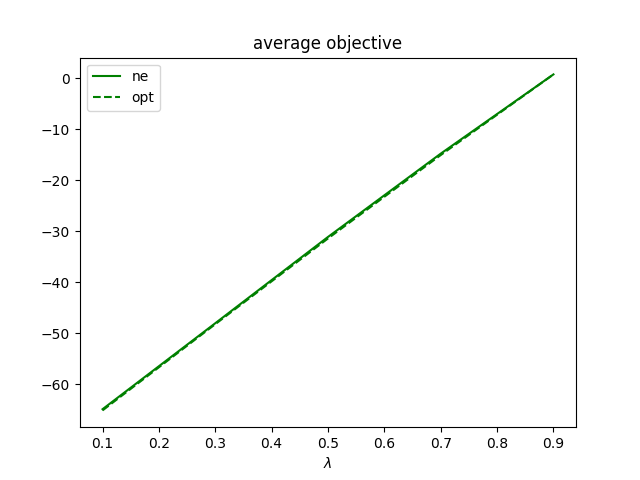
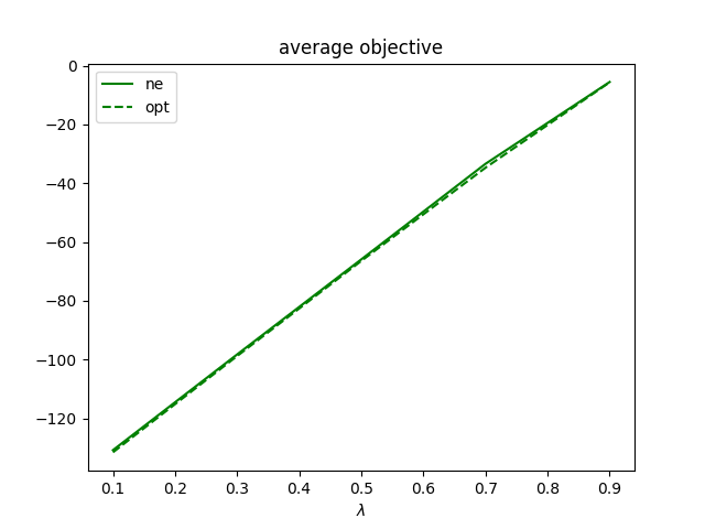
The results are shown in Figures 4-11. In each figure, the horizontal axis is the value which represents the importance of safety for both agents, where lower values of imply that safety is more important. The left plots show the objective value, where lower is better. The middle plots give the time to goal, where lower is, again, better. The right plots show safety margin, where again lower is better. We present average quantities over all agents; the qualitative observations are similar if we consider these at individual agent level.
The first observation is that the difference between socially optimal and equilibrium objective values appears small ((a) plots in Figures 4-11). It is therefore tempting to conclude that equilibrium behavior is similar to socially optimal, but it turns out that this is not the case: in particular, it turns out that the trade-off between efficiency and safety made by the agents in equilibrium is very different from optimal.
Considering next the (b) and (c) columns of the figures, we can observe that systematically performance improves, while safety is often significantly compromised, in equilibrium as compared to a social optimum. The difference is particularly dramatic in the first two scenarios, when the agents are in direct conflict in their quest to reach their respective goals. The gap between optimal and equilibrium safety in the other scenarios tends to be larger for relatively high values of .
Another general observation we can make is that often the solutions with a feedback controller are closer to optimal, particularly from the perspective of safety. The exceptions involve the intersection scenarios, where the gap is larger for higher values of in the feedback controller solution than with the open-loop controller. However, even in these scenarios, the feedback controller yields solutions closer to socially optimal for most values of . This is not surprising: since all agents are concerned about safety, they are more able to dynamically adjust to avoid collisions when some feedback about state is available.
To understand why safety is systematically compromised, consider a single agent’s incentive. Even though an agent is interested in reaching the goal safely, it does not account for the fact that being involved in a crash also crashes the other agent. Thus, in equilibrium safety is compromised relative to social optimum, as agents fail to capture the externalities associated with crashes.






References
- Arkin [1989] Arkin, R.C.: Motor Schema-Based Mobile Robot Navigation (1989)
- Auat Cheein and Carelli [2013] Auat Cheein, F.A., Carelli, R.: Agricultural robotics: Unmanned robotic service units in agricultural tasks. IEEE Industrial Electronics Magazine 7(3), 48–58 (2013)
- Beckmann et al. [1956] Beckmann, M., McGuire, C., Winsten, C.: Studies in the Economics of Transportation (1956)
- Bertsekas [1999] Bertsekas, D.: Nonlinear programming (1999)
- Blackmore et al. [2006] Blackmore, L., Li, H., Williams, B.: A probabilistic approach to optimal robust path planning with obstacles. In: American Control Conference (2006)
- Braess [1968] Braess, D.: Über ein Paradoxon aus der Verkehrsplanung. Unternehmensforschung Operations Research - Recherche Opérationnelle 12(1), 258–268 (dec 1968)
- Chen et al. [2014a] Chen, M., Zhou, Z., Tomlin, C.J.: Multiplayer reach-avoid games via low dimensional solutions and maximum matching. In: American Control Conferenc. pp. 1444–1449 (2014a)
- Chen et al. [2014b] Chen, M., Zhou, Z., Tomlin, C.J.: A path defense approach to the multiplayer reach-avoid game. In: Annual Conference on Decision and Control. pp. 2420–2426 (2014b)
- Craighead et al. [2007] Craighead, J., Murphy, R., Burke, J., Goldiez, B.: A survey of commercial & open source unmanned vehicle simulators. In: Proceedings - IEEE International Conference on Robotics and Automation. pp. 852–857 (2007)
- DeSouza and Kak [2002] DeSouza, G.N., Kak, A.C.: Vision for mobile robot navigation: A survey. IEEE Transactions on Pattern Analysis and Machine Intelligence 24(2), 237–267 (2002)
- Elfes [1989] Elfes, A.: Using occupancy grids for mobile robot perception and navigation. Computer 22(6), 46–57 (1989)
- Geibel and Wysotzki [2005] Geibel, P., Wysotzki, F.: Risk-sensitive reinforcement learning applied to control under constraints. J. Artif. Intell. Res. 24, 81–108 (2005)
- Jonsson and Rovatsos [2011] Jonsson, A., Rovatsos, M.: Scaling up multiagent planning: A best-response approach. In: ICAPS (2011)
- Jordán et al. [2017] Jordán, J., Torreno, A., de Weerdt, M., Onaindia, E.: A better-response strategy for self-interested planning agents. Applied Intelligence pp. 1–21 (2017)
- LaValle [2000] LaValle, S.M.: Robot motion planning: A game-theoretic foundation. Algorithmica 26(3-4), 430–465 (2000)
- Mahony and Kumar [2012] Mahony, R., Kumar, V.: Aerial robotics and the quadrotor. IEEE Robotics and Automation Magazine 19(3), 19 (2012)
- Oldewurtel et al. [2008] Oldewurtel, F., Jones, C.N., Morari, M.: A tractable approximation of chance constrained stochastic mpc based on affine disturbance feedback. In: IEEE Conference on Decision and Control. pp. 4731–4736 (2008)
- Pigou [1932] Pigou, A.: The economics of welfare, 1920. McMillan&Co., London (1932)
- Rosenschein and Zlotkin [1994] Rosenschein, J.S., Zlotkin, G.: Rules of encounter: designing conventions for automated negotiation among computers. MIT press (1994)
- Roughgarden and Tardos [2000] Roughgarden, T., Tardos, E.: How bad is selfish routing? Proceedings 41st Annual Symposium on Foundations of Computer Science 49(2), 1–26 (2000)
- Schmeidler [1973] Schmeidler, D.: Equilibrium points of nonatomic games. Journal of Statistical Physics 7(4), 295–300 (1973)
- Shen et al. [2008] Shen, D., Chen, G., Cruz, J.B., Blasch, E.: A game theoretic data fusion aided path planning approach for cooperative UAV ISR. In: Aerospace Conference. pp. 1–9 (2008)
- Stone and Veloso [2000] Stone, P., Veloso, M.: Multiagent systems: A survey from a machine learning perspective. Autonomous Robots 8(3), 345–383 (2000)
- Wardrop [1952] Wardrop, J.G.: Road paper. some theoretical aspects of road traffic research. Proceedings of the institution of civil engineers 1(3), 325–362 (1952)