Exploiting Intelligent Reflecting Surfaces in NOMA Networks: Joint Beamforming Optimization
Abstract
This paper investigates a downlink multiple-input single-output intelligent reflecting surface (IRS) aided non-orthogonal multiple access (NOMA) system, where a base station (BS) serves multiple users with the aid of IRSs. Our goal is to maximize the sum rate of all users by jointly optimizing the active beamforming at the BS and the passive beamforming at the IRS, subject to successive interference cancellation decoding rate conditions and IRS reflecting elements constraints. In term of the characteristics of reflection amplitudes and phase shifts, we consider ideal and non-ideal IRS assumptions. To tackle the formulated non-convex problems, we propose efficient algorithms by invoking alternating optimization, which design the active beamforming and passive beamforming alternately. For the ideal IRS scenario, the two subproblems are solved by invoking the successive convex approximation technique. For the non-ideal IRS scenario, constant modulus IRS elements are further divided into continuous phase shifts and discrete phase shifts. To tackle the passive beamforming problem with continuous phase shifts, a novel algorithm is developed by utilizing the sequential rank-one constraint relaxation approach, which is guaranteed to find a locally optimal rank-one solution. Then, a quantization-based scheme is proposed for discrete phase shifts. Finally, numerical results illustrate that: i) the system sum rate can be significantly improved by deploying the IRS with the proposed algorithms; ii) 3-bit phase shifters are capable of achieving almost the same performance as the ideal IRS; iii) the proposed IRS-aided NOMA systems achieve higher system sum rate than the IRS-aided orthogonal multiple access system.
I Introduction
Recently, intelligent reflecting surface (IRS) aided transmission has drawn significant attention due to its superior performance in enhancing spectrum efficiency (SE) and energy efficiency (EE) for wireless communication networks [2, 3]. An IRS is a planar array comprising a large number of low cost passive reflecting elements, which can passively reflect the incident electromagnetic wave and simultaneously change its amplitude and phase shift [4]. With this new degree-of-freedom (DoF), an IRS can be deployed to create an additional reflection link when the transmitter and receiver are blocked by obstacles. Compared with conventional relaying technologies (e.g amplify-and-forward (AF) and decode-and-forward (DF) relays), IRSs require much less energy consumption due to the nearly passive characteristics [5]. Therefore, IRS technology has drawn tremendous attention from both academia and industry, and has been regarded as a promising solution in future 6G networks [5, 6].
Non-orthogonal multiple access (NOMA) is one of the key technologies in future wireless communication networks due to its higher SE achievement, user fairness guarantee, and massive connectivity support [7, 8]. The key idea of NOMA is to serve multiple users in the same resource block (i.e., time, frequency and code), where superposition coding (SC) and successive interference cancellation (SIC) are applied at the transmitter and receiver, respectively [9, 10]. Specifically, users who have better channel conditions can remove the intra-channel interference. In the current literature, the performance gains of NOMA over orthogonal multiple access (OMA) have been investigated in various scenarios, such as cognitive radio [11] and millimeter wave communication [12]. Sparked by the aforementioned benefits of the IRS and NOMA, we explore in this paper the potential performance improvement brought by effectively integrating NOMA technology with IRS-aided communications.
I-A Prior Works
I-A1 Studies on Single-Input Single-Output (SISO)-NOMA Systems
Prior works on NOMA in the single-antenna scenario have studied various aspects such as user fairness, user grouping schemes, power allocation design. For example, Timotheou et al. [13] studied the power allocation problem with the aim of guaranteeing fairness among served users. Ding et al. [14] further analyzed the performance of NOMA in both a fixed power allocation system (F-NOMA) and cognitive radio inspired NOMA (CR-NOMA) under different user pairing schemes. Choi et al. [15] proposed optimal power allocation schemes in a two-user downlink NOMA system, where the max-sum rate and max-min rate with proportional fairness objective functions were considered. A dynamic power allocation scheme (D-NOMA) for both downlink and uplink transmission was proposed by Yang et al. [16] while satisfying different users’ quality of service (QoS) requirements, which demonstrated that D-NOMA outperforms F-NOMA and CR-NOMA in terms of communication rate and fairness. Moreover, Liu et al. [17] studied cooperative NOMA with simultaneous wireless information and power transfer (SWIPT) technology, where near users with energy harvesting act as relays to enhance the received signal quality of far users. Fang et al. [18] studied multi-subcarrier downlink NOMA to maximize the EE by jointly optimizing subchannel assignment and power allocation, where a low complexity algorithm was designed based on matching theory and DC programming method. Full-duplex multi-subcarrier systems were investigated by Sun et al. [19], where the optimal power allocation and user scheduling scheme was designed by applying monotonic optimization theory.
I-A2 Studies on Multiple-Input Multiple-Output (MIMO)-NOMA Systems
Hanif et al. [20] proposed an effective beamforming design algorithm to maximize the system sum rate, where a multi-antenna base station (BS) served multiple single-antenna users through the NOMA protocol. Considering multiple antenna techniques at both the BS and users, Ding et al. [21] studied the precoding and detection designs, where users are partitioned into several clusters and NOMA transmission was applied in each cluster. User fairness in MIMO-NOMA systems was investigated by Liu et al. [22], where three user clustering schemes with power allocation designs were proposed to guarantee user fairness with a lower computation complexity. Furthermore, a general framework for MIMO-NOMA in both downlink and uplink transmission was proposed in [23]. By adopting the signal alignment technique, the MIMO-NOMA transmission can be divided into several independent single-antenna cases for NOMA implementations. Ali et al. [24] optimized user scheduling, beamforming vectors and power allocation in multiuser MIMO-NOMA networks, where zero-forcing beamforming was designed with the equivalent channel power gain of each cluster in order to cancel the inter-cluster interference. To investigate secure NOMA transmission, Liu et al. [25] analyzed the secrecy performance with stochastic geometry in both single-antenna and multiple-antenna scenarios. Particularly, artificial noise was invoked to enhance secrecy performance in multiple-antenna NOMA communication. Alavi et al. [26] investigated beamforming design with different objective functions based on perfect and imperfect channel state information (CSI). To further investigate the application of MIMO-NOMA, Ding et al. [27] proposed a precoding design scheme for Internet of Things (IoT) transmission scenarios. Wang et al. [28] applied NOMA to millimeter-wave communication with the concept of beamspace MIMO, which demonstrated that NOMA can achieve higher system SE and EE than the conventional beamspace MIMO communication.
I-A3 Studies on IRS-aided Systems
In contrast to conventional communication systems, the channel response can be modified by deploying an IRS. Driven by this unique characteristic, some initial studies showed how to enhance system performance by designing the passive beamforming at the IRS. Wu et al. [29] developed alternating algorithms for beanmforming design at both the BS and IRS to minimize the total transmit power, where the passive beamforming was designed with the semidefinite relaxation (SDR) approach. To maximize the EE in the IRS-assisted multi-user multiple-input single-output (MISO) system, Huang et al. [30] proposed two efficient algorithms by jointly optimizing the power allocation and IRS phase shifts while considering a realistic IRS power consumption model. Yu et al. [31] maximized the SE for an IRS-aided point-to-point MISO transmission, where the non-convex unit modulus constraint at the IRS was handled by the fixed point iteration and manifold optimization methods. Taha et al. [32] proposed a novel IRS architecture with several RF chains connected to the IRS controller. Based on this, two channel estimation methods were developed by utilizing compressive sensing and deep learning tools. Chen [33] invoked IRSs for secure transmission in a downlink MISO system coexisting with multiple eavesdroppers. Cui et al. [34] further revealed that secure transmission can still be achieved with IRSs even when the eavesdropping channel is stronger than the legitimate channel. With the target of maximizing the sum rate of the IRS-aided system, the joint optimization of active and passive beamforming was solved by utilizing the deep reinforcement learning in [35]. A novel IRS-aided NOMA communication model was proposed in [36], where IRSs were deployed at cell edge regions to maximize the total number of served users. Yang et al. [37] investigated the max-min rate problem in both SISO and MISO IRS-aided NOMA systems. Fu et al. [38] studied the total transmit power minimization problem in the downlink MISO NOMA IRS-aided system, where a penalty-based iterative algorithm was proposed to optimize the passive beamforming vector. For practical implementation, IRS elements with finite resolution phase shifters were considered in [39, 40, 41, 42, 43]. Huang et al. [39] studied the EE maximization problem with low resolution IRS elements by invoking the quantization method. The minimum requirement on the number of resolution bits of the IRS was derived by Han et al. [40] to achieve an acceptable ergodic SE performance. A successive refinement algorithm was proposed by Wu et al. [41] for the discrete IRS phase shifts design. Guo et al. [42] investigated the weighted sum-rate maximization problem in the IRS-assisted multi-user MISO system, where three efficient algorithms were developed under different IRS element assumptions. You et al. [43] jointly considered the channel estimation and passive beamforming design with discrete phase shifts at the IRS.
I-B Motivation and Contributions
It is known that the success of SIC based detection at the users in NOMA transmission is mainly determined by the channel power gains of different users. However, in IRS-aided systems, the channel response can be artificially modified by adjusting the reflection coefficients, which presents new challenges to the application of NOMA. Although few works investigated IRS-aided NOMA systems[36, 37, 38], to the best of our knowledge, there is no existing work on the sum rate optimization problem in the MISO IRS-aided NOMA system. In the aforementioned research contributions [29, 37], the SDR approach has been invoked for passive beamforming design. However, the Gaussian randomization approach should be adopted when the obtained solution is not rank-one, which only provides an approximate solution. The weighted sum-rate maximization problem has been studied in [42] for a multi-user IRS-assisted MISO system under different IRS constraints. However, the proposed methods cannot be directly applied in the IRS-aided NOMA system. The main challenges of IRS-aided NOMA networks are as follows: i) for multi-antenna NOMA transmission, the decoding order is not determined by the users’ channel power gains order, since additional decoding rate conditions need to be satisfied to guarantee successful SIC [10]; ii) both the active and passive beamforming in IRS-aided NOMA affect the decoding order among users, which makes the decoding order design and beamforming design highly coupled.
Driven by the above challenges, in this article, we investigate the joint beamforming design at both the BS and IRS to maximize the sum rate in downlink MISO IRS-aided NOMA systems. Our main contributions of this paper are summarized as follows:
- •
We propose a downlink MISO IRS-aided NOMA framework, in which the IRS is utilized for SE enhancement. Based on the proposed framework, we formulate a joint active and passive beamforming design problem to maximize the system sum rate, subject to total transmit power, SIC decoding rate constraints, user rate fairness constraints and various constraints on IRS reflecting elements, which are defined as ideal and non-ideal IRS.
- •
For the ideal IRS, both the reflection amplitudes and phase shifts can be designed. We develop an iterative algorithm using alternating optimization (AO), where the non-convex active and passive beamforming design subproblems are alternately solved by utilizing the successive convex approximation (SCA) technique. In addition, we prove that a rank-one solution can be always obtained for active beamforming design.
- •
For the non-ideal IRS, the reflection amplitudes are fixed with constant values and only phase shifts can be designed, including continuous phase shifts and discrete phase shifts. We first invoke a novel sequential rank-one constraint relaxation (SROCR) approach to deal with passive beamforming design problem with continuous phase shifts. In contrast to the SDR approach, the proposed algorithm can find a locally optimal rank-one solution. Then, for discrete phase shifts, the passive beamforming is designed by leveraging the quantization method with some modifications.
- •
We show that the proposed algorithms are capable of achieving promising sum rate gains, compared to both the conventional system without the IRS and the IRS-aided OMA system. We also demonstrate that the performance gap between the 3-bit phase shifters and the ideal IRS is negligible.
I-C Organization and Notations
The rest of this paper is organized as follows. Section II presents the system model and problem formulation. In Section III and Section IV, we propose efficient algorithms for the active and passive beamforming design under ideal and non-ideal IRS assumptions. Section V presents the numerical results to validate the effectiveness of the proposed designs. Finally, Section VI concludes the paper.
Notations: Scalars, vectors and matrices are denoted by lower-case letters, bold-face lower-case and upper-case letters, respectively. Real-valued and complex-valued matrices with the space of are denoted by and , respectively. All -dimensional complex Hermitian matrices are denoted by . All -dimensional real symmetric matrices are denoted by . represents an identity matrix. The rank and the trace of matrix are denoted by and . represents is a positive semidefinite matrix. , and denote the transpose, the conjugate transpose and the diagonal matrix of vector , respectively. extracts the real value of a complex variable.
II System Model and Problem Formulation
II-A System Model

As illustrated in Fig. 1, we consider a downlink MISO IRS-aided NOMA system, which consists of an -antenna base station, single-antenna users and an IRS equipped with passive reflecting elements. In practice, the IRS is managed by the BS through a smart controller which exchanges information and coordinates transmission. Due to the “double fading” effect [44], the reflection link suffers from more severe path loss than the direct link. The power of the signals reflected by the IRS two or more times is much smaller than that of signals reflected one time and can be ignored [29, 42]. The CSI of all channels are assumed to be perfectly known at the BS11 1 The involved CSI can be efficiently obtained by the recently proposed channel estimation techniques for IRS-aided systems [32, 43]. The results in this work actually provide a theoretical performance upper bound for the considered system. Our future work will relax this perfect CSI assumption by considering robust beamforming design. and the quasi-static flat-fading model is considered22 2 In this paper, the users are assumed to be static or moving at a low speed in the considered networks. As a result, the channels would remain unchanged for a long time duration and the time consumption for channel acquisitions can be ignored.. Let denote the diagonal reflection coefficients matrix of the IRS with and , where and denote the reflection amplitude and phase shift of the th reflecting element on the IRS, respectively. Depending on the amplitude and phase shift features of reflecting elements, two sets of IRS assumptions are considered as follows [45]:
- •
Ideal IRS: In this scenario, the reflecting elements can be optimized with arbitrary continuous amplitudes and phase shifts. Thus, the feasible set of can be expressed as
(1) - •
Non-ideal IRS: In this scenario, the reflection amplitude is fixed with a constant value, such as . We further discuss the two scenarios of continuous phase shifts and discrete phase shifts. In particular, the feasible set of for continuous phase shifts can be expressed as
(2) and the feasible set of for discrete phase shifts with resolution bits can be expressed as
(3) where .
The channels from the BS to user , the IRS to user and the BS to IRS are denoted by , and , respectively. Let denote the information-bearing symbol for the th user with zero mean and unit variance. Therefore, the complex baseband signal transmitted from the BS can be expressed as , where represents the active beamforming vector for the th user. Then, the received signal at user can be expressed as
| (4) |
where is the additive white Gaussian noise (AWGN) at user with zero mean and variance .
Based on the NOMA principle, each user tries to employ SIC to remove the intra-cell interference. In SISO NOMA systems, the optimal decoding order among users are determined by the channel power gains. The user with a stronger channel power gains can decode the user’s signal who has a weaker channel power gain. However, this ordering method cannot be applied in a MISO NOMA system since the channel responses can be modified with the introduced IRS, which can change the decoding order to be any one of all the different decoding orders. Let denote the decoding order of user . For instance, if , then user is the th signal to be decoded. Based on this order, user first successively decodes the signal of each user with before decoding its own signal, and treats the signal of each user with as interference [7, 9]. Compared with the conventional communication system, the implementation of NOMA technology imposes additional complexity since the users have to decode information intended for some of the other users. Therefore, the achievable signal-to-interference-plus-noise ratio (SINR) at user to decode its own signal can be expressed as
| (5) |
The corresponding achievable rate at user to decode it own signal is .
Furthermore, for any users and which satisfy , the SINR at user to decode user ’s signal can be expressed as
| (6) |
The corresponding achievable rate at user to decode user ’s signal is .
It is worth noting that in order to guarantee that the SIC can be performed successfully, the achievable rate at user to decode user ’s signal should be no less than the achievable rate at user to decode it own signal [10]. Then, we have the following SIC decoding rate constraints
| (7) |
In addition, to guarantee rate fairness among all users, the following conditions should be satisfied with given decoding orders
| (8) |
From equation (5), it can be observed that users with higher decoding orders receive less or no interference from other users due to the SIC. The inequalities in (8) avoid the case that most of the radio resources are allocated to some of the higher decoding order users. With the above inequalities, the received signal power of users in lower decoding orders is made greater than that of users with higher decoding orders. As a result, a reasonable communication rate can be achieved at users in lower decoding orders, which is capable of maintaining the rate fairness among users.
For example, let us consider the two-user case. If the decoding order is set as , then SIC decoding and rate fairness conditions can be expressed as
| (9a) | ||||
| (9b) | ||||
For the three-user case with the decoding order , the SIC decoding rate conditions at user 2 and user 3 and rate fairness condition among all users can be expressed as
| (10a) | ||||
| (10b) | ||||
It is worth noting that when users are served in the IRS-aided NOMA system, there will be SIC decoding rate constraints and rate fairness constraints, which depend on not only the active beamforming coefficients at the BS, but also the combined channel (which depends on the passive beamforming vector at the IRS).
II-B Problem Formulation
Our goal is to maximize the sum rate of all users by jointly optimizing the active beamforming coefficients at the BS and the passive beamforming vector at the IRS, subject to the total power constraint, the SIC decoding rate and the user rate fairness constraints under different IRS assumptions. The optimization problem can be formulated as
| (11a) | ||||
| (11b) | ||||
| (11c) | ||||
| (11d) | ||||
| (11e) | ||||
| (11f) | ||||
where denotes the set of all possible SIC decoding orders and denotes the total transmit power. Constraint (11b) guarantees that the SIC can be performed successfully. Constraint (11c) is the total transmission power constraint and (11d) represents the considered IRS assumption. Constraint (11f) guarantees rate fairness among all users. It is worth noting that Problem (P1) is always feasible under any given , since we consider the rate fairness constraints instead of the strict QoS constraints [29, 30]. However, Problem (P1) is a highly-coupled non-convex problem even with convex set , which makes it hard to find the global optimal solution. In the following, efficient algorithms are developed based on the AO method to derive a high quality suboptimal solution.
III Ideal IRS Case
In this section, we focus on the Problem (P1) with the ideal IRS. Before solving this problem, we first transform (P1) into a more tractable form. Let and . Then, we have . Furthermore, we introduce slack variables and such that
| (12) |
| (13) |
Then, the decoding rate can be expressed as
| (14) |
With the above variable definitions, Problem (P1) can be transformed into
| (15a) | ||||
| (15b) | ||||
| (15c) | ||||
| (15d) | ||||
| (15e) | ||||
| (15f) | ||||
| (15g) | ||||
Proposition 1.
Problem (P2) is equivalent to Problem (P1).
Proof.
Without loss of optimality to Problem (P1), constraints (15b), (15c) and (15d) can be met with equality. Specifically, when , assume that if any of the constraints in (15b) is satisfied with strict inequality, then we can always increase to make the constraint (15b) satisfied with equality while increasing the objective function’s value. Furthermore, suppose that (15c) and (15d) are satisfied with strict inequality, then we can always reduce or increase to make all constraints satisfied with equality, which in turn increases the value of the right-hand-side (RHS) in (15b) and increases the objective function’s value. When , assume that if any of the constraints in (15b) is satisfied with strict inequality, then we can always increase without changing the objective function’s value of (P1). Therefore, Problem (P2) is equivalent to Problem (P1). ∎
However, Problem (P2) is still a non-convex optimization problem since the decoding order , the active beamforming coefficients and the passive beamforming vector are highly-coupled. Since the total number of decoding order combinations is a finite value, the optimal sum rate can be obtained by solving Problem (P2) with any one of decoding orders at first and selecting the maximum objective function’s value among all decoding orders. For a given decoding order, the sum rate maximization problem in (P2) with the ideal IRS is reduced to
| (16a) | ||||
| (16b) | ||||
| (16c) | ||||
In order to tackle the highly-coupled non-convex terms in Problem (P3), we decompose the original problem into the two subproblems of active beamforming optimization and passive beamforming optimization, which can be efficiently solved by the SCA technique as described next.
III-A Active Beamforming Optimization
Define , which satisfy and . Under any given feasible passive beamforming vector , the active beamforming optimization problem can be written as
| (17a) | ||||
| (17b) | ||||
| (17c) | ||||
| (17d) | ||||
| (17e) | ||||
| (17f) | ||||
| (17g) | ||||
| (17h) | ||||
Lemma 1.
For and , is a convex function with respect to and .
Proof.
It is easy to prove lemma 1 by showing that the Hessian matrix of function is positive semidefinite when and . As a result, is a convex function. ∎
Problem (P3.1) is a non-convex problem due to the non-convex constraints (15b) and (17g). Based on Lemma 1, the RHS of (15b) is a joint convex function with respect to and . By applying the first-order Taylor expansion, the lower bound at given local points can be expressed as
| (18) |
Then, Problem (P3.1) is approximated as the following problem
| (19a) | ||||
| (19b) | ||||
| (19c) | ||||
Note that the remaining non-convexity of (P3.2) is the rank-one constraint (17g). To tackle this issue, we have the following theorem
Theorem 1.
Without loss of optimality, the obtained solution to Problem (P3.2) without rank-one constraint (17g) can always satisfy .
Proof.
See Appendix A. ∎
Based on Theorem 1, we can always obtain a rank-one solution by solving (P3.2) by ignoring the rank-one constraint (17g). As a result, the relaxed problem is a convex semidefinite program (SDP), which can be efficiently solved via standard convex problem solvers such as CVX [46]. Note that the objective function’s value obtained from Problem (P3.2) in general provides a lower bound on that of Problem (P3.1) due to the replacement of the lower bounds (18). After solving (P3.2), the active beamforming coefficients can be obtained through Cholesky decomposition, e.g. .
III-B Passive Beamforming Optimization with
Given any feasible active beamforming vectors , the passive beamforming optimization problem with ideal IRS can be written as
| (20a) | ||||
| (20b) | ||||
Problem (P3.3) is a non-convex problem due to non-convex constraints (15b), (15c) and (15f). In the previous subsection, we have already showed how to tackle the non-convex constraint (15b). For the non-convex constraint (15c), the RHS is a convex function with respect to , the lower bound with the first-order Taylor expansion at the given local point can be expressed as
| (21) |
Similarly, for the non-convex constraint (15f), the left hand side (LHS) can be replaced with the lower bound in (21). Then, the passive beamforming optimization problem is approximated as the following problem
| (22a) | ||||
| (22b) | ||||
| (22c) | ||||
| (22d) | ||||
| (22e) | ||||
Now, it is easy to verify that Problem (P3.4) is a convex problem, which can be efficiently solved via standard convex problem solvers such as CVX [46]. Similarly, the objective function’s value obtained from (P3.4) serves as a lower bound on that of (P3.3).
III-C Proposed Algorithm, Complexity and Convergence
Based on the above two subproblems, we propose an iterative algorithm for Problem (P3) with the ideal IRS by utilizing the AO method. Specifically, the active beamforming coefficients and the passive beamforming vector are alternately optimized by solving Problem (P3.2) and (P3.4), where the solutions obtained after each iteration are used as the input local points for the next iteration. The details of the proposed algorithm are summarized in Algorithm 1. According to [47], the complexity of the SDP subproblem for active beamforming design is , where denotes the accuracy. The complexity of the subproblem for passive beamforming design with the interior-point method is [48]. Then, the total complexity of Algorithm 1 is
, where denotes the number of iterations for Algorithm 1.
ÓÃÀ´¿ØÖÆλÖã¬Í¬Ê±ÀûÓÃ
½øÐл»ÐÐ
Initialize a decoding order and feasible solutions to (P3), .
Next, we demonstrate the convergence of Algorithm 1. Define as the objective function’s value of Problem (P3) in the th iteration. First, for Problem (P3.2) with given passive beamforming vector in step 2 of Algorithm 1, we have
| (23) |
where represents the objective function’s value of Problem (P3.2). follows the fact that the first-order Taylor expansions are tight at the given local points in Problem (P3.2); holds since Problem (P3.2) is solved optimally; holds due to the fact that the objective function’s value of Problem (P3.2) serves as a lower bound on that of (P3.1). This suggests that the objective function’s value of Problem (P3.1) is non-decreasing after each iteration.
Similarly, for Problem (P3.4) with given active beamforming coefficients in step 3 of Algorithm 1, we have
| (24) |
where represents the objective function’s value of Problem (P3.4).
As a result, based on (23) and (24), we obtain that
Remark 1.
Equation (III-C) indicates that the objective function’s value of Problem (P3) is non-decreasing after each iteration. Since the system sum rate is upper bounded by a finite value, the proposed algorithm is guaranteed to converge.
IV Non-Ideal IRS Case
In this section, we solve Problem (P2) with non-ideal IRS. The sum rate maximization problem in (P2) for a given decoding order can be written as
| (26a) | ||||
| (26b) | ||||
| (26c) | ||||
To tackle this problem, we decompose (P4) into two subproblems. Since the active beamforming coefficients can still be optimized by solving (P3.2), we only need to focus on how to optimize the passive beamforming vector with the case of or . In the following, we first invoke a novel SROCR approach [49] to deal with the passive beamforming optimization with continuous phase shifts. Then, the passive beamforming design for discrete phase shifts is handled with the quantization-based scheme.
IV-A Passive Beamforming Optimization with
Equipped with continuous phase shifters, each element on the IRS has a constant reflection amplitude, i.e. . To tackle the unit modulus constraint, we define which satisfies , and . Then, for any given feasible active beamforming coefficients , Problem (P4) can be written as
| (27a) | ||||
| (27b) | ||||
| (27c) | ||||
| (27d) | ||||
| (27e) | ||||
| (27f) | ||||
| (27g) | ||||
| (27h) | ||||
The non-convexity of (P4.2) lies in the non-convex constraint (15b) and the rank-one constraint (27g). Similarly, the non-convex constraint (15b) can be replaced with its lower bound in (18). For the rank-one constraint (27g), the conventional approach is applying SDR [29, 37], where we first solve the problem by ignoring the rank-one constraint, and then construct a rank-one solution with Gaussian randomization method if the solution obtained from the relaxed problem is not rank-one. One drawback of this approach is that the constructed rank-one solution is normally a suboptimal solution or even infeasible for the original problem. The objective function’s value may not be non-increasing after each iteration, which results in the convergence of the proposed algorithm cannot be guaranteed. Driven by this issue, we propose a novel SROCR-based algorithm to obtain a local optimal rank-one solution. The basic framework of the SROCR approach [49] can be found in Appendix B. By replacing the non-convex term in (15b) with the lower bound in (18), Problem (P4.1) can be written as
| (28a) | ||||
| (28b) | ||||
| (28c) | ||||
| (28d) | ||||
Now, Problem (P4.2) satisfies the general framework for the SROCR approach, which is shown in Problem (P) in Appendix B. Therefore, we apply the SROCR approach to solve Problem (P4.2). First, we replace the non-convex rank-one constraint with the relaxed convex constraint which controls the largest eigenvalue to trace ratio of with the parameter . Thus, the relaxed optimization problem can be expressed as
| (29a) | ||||
| (29b) | ||||
| (29c) | ||||
where is the eigenvector corresponding to the largest eigenvalue of and is the obtained solution in the th iteration with . It can be verified that Problem (P4.3) is a convex problem that can be efficiently solved with convex optimization software, such as CVX [46]. By increasing the parameter from 0 to 1 after each iteration, we can derive a locally optimal rank-one solution for (P4.2). The details of solving Problem (P4.2) are summarized in Algorithm 2. Similarly, the objective function’s value obtained from (P4.2) serves as a lower bound on that of (P4.1) due to the replacement of non-convex terms with their lower bounds. After solving (P4.2), the passive beamforming vector for the continuous phase shifts case can be obtained through Cholesky decomposition, e.g. .
ÓÃÀ´¿ØÖÆλÖã¬Í¬Ê±ÀûÓÃ
½øÐл»ÐÐ
Initialize convergence thresholds , and feasible to problem (P4.2), .
Solve the relaxed problem (P4.3) with , the obtained solution is denoted by , initialize the step size .
IV-B Passive Beamforming Optimization with
In this subsection, we discuss the passive beamforming design with discrete phase shifts. The optimization problem becomes a combinatorial optimization problem. Though the optimal solution can be obtained via an exhaustive search, it requires a prohibitive complexity since the number of elements on the IRS is usually large. Recall the fact that elements in and both follow the unit modulus constraint. Hence, we can directly quantize the obtained solution in the continuous phase shifts case to the nearest feasible point in the discrete phase shifts case as follows
where However, the obtained solution with quantization method may be not a locally optimal solution. In order to make the objective function’s value to be non-increasing after each iteration for , we update only when .
IV-C Proposed Algorithm, Complexity and Convergence
Similarly, we propose an iterative algorithm for Problem (P4) with non-ideal IRS by utilizing the AO method. The details of the proposed algorithm are summarized in Algorithm 3. The complexity of the SDP subproblem for the passive beamforming optimization is , where denotes the number of iterations for Algorithm 2 with the SROCR approach and denotes the accuracy. The total complexity of Algorithm 3 is
where denotes the number of iterations for Algorithm 3 [47]. It can be seen that the computational complexity of the algorithm with the non-ideal IRS is larger than that with the ideal IRS. The convergence of Algorithm 3 can be proved in a similar way as Algorithm 1.
ÓÃÀ´¿ØÖÆλÖã¬Í¬Ê±ÀûÓÃ
½øÐл»ÐÐ
Initialize a decoding order and feasible solutions to (P4), .
Remark 2.
In practical applications, it is costly to deploy IRSs with ideal case or continuous phase shifts due to hardware limitations. However, it is still important to analyze the cases of and since they provide theoretical performance upper bounds to the case of .
IV-D Passive Beamforming Optimization with 1-Bit Phase Shifters
As described earlier, the quantization method can provide a feasible solution for the passive beamforming design in the discrete phase shifts case. However, this method may experience substantial performance losses with low resolution phase shifters, e.g., . To overcome this drawback, we investigate the passive beamforming design with 1-bit phase shifters in this subsection. Specifically, the passive beamforming optimization problem of 1-bit phase shifters under given can be written as
| (33a) | ||||
| (33b) | ||||
| (33c) | ||||
Problem (P4.4) is a Boolean quadratic problem (BQP). Similarly, let which satisfies , , and . Then, Problem (P4.4) can be expressed as
| (34a) | ||||
| (34b) | ||||
| (34c) | ||||
| (34d) | ||||
| (34e) | ||||
Problem (P4.5) can be regarded as a non-convex rank-one optimization problem with a real symmetric matrix set, which can also be solved by the proposed SROCR-based algorithm.
Remark 3.
Since a locally optimal rank-one solution can be obtained for the passive beamforming optimization with the SROCR approach, the sum rate of 1-bit phase shifters obtained by the SROCR-based algorithm will be no worse than that of the quantization-based scheme.
V Simulation Results
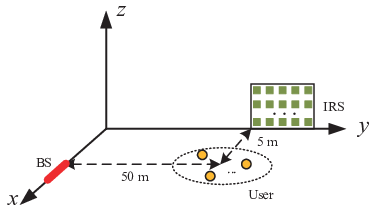
In this section, simulation results are provided to validate the effectiveness of the proposed algorithms. As illustrated in Fig. 2, we consider a three-dimensional (3D) coordinate system, where the BS and IRS are equipped with a uniform linear array (ULA) located on the -axis and a uniform planar array (UPA) located parallel to the plane, respectively. The reference antennas at the BS and IRS are set at meters and meters, respectively. The antenna spacing is half wavelength. The number of IRS elements is set as , where and denote the number of IRS elements along the -axis and -axis, respectively. We set and increase linearly with . The served users are randomly and uniformly distributed in a circle region centered at with the radius of 3 m. The distances for the direct BS-user link, the BS-IRS link and the IRS-user link are denoted by , and , respectively. The distance-dependent path loss for all channels is modeled as
| (35) |
where dB denotes the path loss at the reference distance meter, denotes the link distance and denotes the path loss exponent. For small scale fading, the Rayleigh fading channel model and the Rician fading model are assumed for the direct BS-user link and the BS-IRS/IRS-user links, respectively. Then, the corresponding channel coefficients can be expressed as
| (36a) | ||||
| (36b) | ||||
| (36c) | ||||
where and denote the Rician factors, and denote the deterministic LoS components, , and denote the Rayleigh fading components. From (36b) and (36c), it can be observed that the reflection link suffers from the “double-fading” effect [44]. In this paper, the path loss exponents for the direct link, AP-IRS link and IRS-user link are set to be , and , respectively. The Rician factors are dB. The noise power is given by with bandwidth = 1 MHz and the effective noise power density of dbm/Hz [29]. All simulation results are obtained by averaging over 100 independent channel realizations. To strike a balance between the obtained performance and computational complexity, the convergence threshold of the proposed algorithms is set to be .
V-A Convergence of Proposed Algorithms
In Fig. 3, we first provide the convergence of Algorithm 1 and Algorithm 3 for , , and dBm. The initial active beamforming coefficients and passive beamforming vector are obtained with the following method33 3 It is worth noting that more sophisticated initialization schemes may further enhance the convergence speed and the attainable performance of the proposed algorithms, but this is beyond the scope of this paper.
- •
Passive beamforming initialization: In the and cases, the phase shift of each element is uniformly distributed between and the reflection amplitude is set to be 1. In the case, the initial passive beamforming vector is obtained by quantizing the random continuous phase shifts to the discrete phase shifts.
- •
Active beamforming initialization: Given the initial passive beamforming vector, the active beamforming vectors are generated with equal power allocation , while satisfying the SIC decoding rate conditions and user rate fairness constraints.
From Fig. 3, it is observed that the sum rate of the proposed algorithms increase quickly with the number of iterations. The proposed SCA and SROCR based algorithms converge with around 6 and 12 iterations, respectively, which is consistent with Remark 1.

V-B Impact of the IRS
In order to demonstrate the benefits brought by deploying the IRS, we compare the proposed algorithms with the following benchmark schemes
- •
- •
Random phase shifts: In this case, the phase shifts of IRS elements are set with random values in . Then, we only optimize the active beamforming at the BS with the combined channels by solving Problem (P3.2).
- •
Without IRS: In this case, the BS served multiple users without the aid of an IRS. The active beamforming vectors are optimized with BS-user channels by solving Problem (P3.2).


V-B1 Sum Rate versus the Number of IRS Reflecting Elements
In Fig. 5, we provide the sum rate versus the number of IRS reflecting elements for , and dBm with different schemes. It is firstly observed that the sum rate of all IRS-aided schemes increase with the increase of , while the sum rate of the “Without IRS” scheme remains unchanged. This is expected since a higher array gain can be achieved with a larger number of IRS reflecting elements. Moreover, the proposed schemes and the “SDR approach” both significantly outperform the “Random phase shifts” scheme, which unveils the importance of IRS phase shifts optimization. It is also observed that the performance gain of the proposed SROCR algorithm over the “SDR approach” becomes more pronounced as the number of reflecting elements increases. This is expected since the probability of the obtained solution satisfying the rank-one constraints becomes lower when increases. The Gaussian randomization approach only provides an approximate solution, which results in performance degradation. From the perspective of different IRS assumptions, it is observed that the performance gaps between the case of ideal IRS and continuous phase shifts can be ignored. This is because the amplitudes of the passive beamforming vectors obtained from Algorithm 1 are nearly one. For practical discrete phase shifts , we observe that the performance degradation caused by finite resolution phase shifters decreases as the resolution bit increases. In particular, the performance achieved by the SROCR-based algorithm with 1-bit phase shifters outperforms the quantization-based scheme, which is consistent with Lemma 3. This is because the SROCR-based algorithm is capable of finding a locally optimal rank-one solution.
V-B2 Sum Rate versus Transmit Power
Fig. 5 presents the achieved system sum rate versus the transmit power of different schemes for , and . As illustrated, it is firstly observed that the sum rate of all considered schemes increase with the increase of . However, for achieving the same sum rate, the proposed schemes consume less transmit power than the “Without IRS” scheme. The “SDR approach” only achieves a similar performance as the 2-bit phase shifts case, which also verifies the effectiveness of the proposed SROCR-based algorithm. It is also observed that the “Random phase shifts” scheme only slightly outperforms the “Without IRS” scheme since the IRS phase shifts are not optimized.


V-B3 Sum Rate versus the Number of BS Antennas
Fig. 7 provides the achieved system sum rate versus the number of BS antennas for , and dBm with different schemes. The sum rate of all schemes increase with the increase of since a larger active beamforming gain can be achieved. It is also observed that the proposed algorithms significantly outperform the “Random phase shifts” and “Without IRS” schemes, which underscores the importance of joint active and passive beamforming optimization.
V-B4 Sum Rate versus the Resolution Bits
Fig. 7 illustrates the sum rate versus the number of resolution bits of the IRS phase shifters. The ideal IRS case achieves the best performance, while the discrete case of achieves the worst performance. This is expected since , which is also consistent with Lemma 2. It is also observed that the performance gap between and becomes narrower with the increase of resolution bits. As illustrated, “1-bit” and “2-bit” schemes are capable of achieving around 90% and 95% performance of the ideal IRS case, respectively. Moreover, the performance loss between the “3-bit” scheme and the ideal IRS is negligible.


V-C Impact of Decoding Order
To evaluate the impact of the decoding order on the sum rate, we compare the following schemes: 1) “IRS-NOMA-Exhaust” denotes the proposed algorithms where the optimal decoding order is selected through exhaustive search; 2) “IRS-NOMA-Random” denotes the case where the active and passive beamforming vectors are optimized with a randomly selected decoding order. For both schemes, continuous phase shifts are assumed and , . As illustrated in Fig. 9, the proposed algorithm outperforms the benchmark scheme, which highlights the importance of finding the optimal decoding order. It is worth noting that the proposed algorithms need to search over possible decoding orders, which is acceptable when the number of users is not large. However, when is large, the complexity will be prohibitively high. In this case, some low-complexity ordering methods are required.
V-D Impact of the Number of Users
In Fig. 9, we investigated the sum rate versus the number of users for , where continuous phase shifts are considered. It is observed that the obtained sum rate remains at an almost constant value with the increase of . Though the impact of the number of users on the sum rate is negligible, it implies that a larger number of users results in a lower average user rate. Moreover, it is also found that a higher transmit power or larger number of IRS elements leads to a higher sum rate.
V-E Performance Comparison with OMA
Finally, we compare the proposed IRS-aided NOMA scheme with the IRS-aided OMA scheme. In the IRS-aided OMA scheme, the BS serves all users through time division multiple access with the aid of the IRS, where the active and passive beamforming vectors are jointly optimized to maximize the received signal strength at the served user during each time slot. Fig. 10 depicts the sum rate of both IRS-aided NOMA and IRS-aided OMA schemes for and in the continuous phase shifts case. It is observed that the IRS-aided NOMA scheme significantly outperforms the IRS-aided OMA scheme. This is expected since all users can be served simultaneously through the NOMA protocol compared with the OMA scheme.

VI Conclusion
In this paper, the MISO IRS-aided NOMA system has been investigated. The sum rate maximization problem was formulated by jointly optimizing the active and passive beamforming vectors under various IRS elements assumptions. To tackle these non-convex problems, the original problem was decoupled into two subproblems, namely, active beamforming optimization and passive beamforming optimization. For the ideal IRS case, the two non-convex subproblems were alternately solved by applying the SCA technique. For the non-ideal IRS case, a novel SROCR-based algorithm was proposed to find a locally optimal rank-one solution for continuous phase shifts. A quantization-based scheme was designed for discrete phase shifts. Simulation results showed that significant performance gains can be achieved by the proposed designs compared with non-IRS or IRS-aided OMA systems. It is worth noting that obtaining perfect CSI is a challenging task for IRS-aided networks, our future research will consider robust beamforming design with imperfect CSI.
Appendix A: Proof of Theorem 1
Problem (P3.2) is a convex problem. Therefore, the optimal solution is characterized by the KKT conditions. Specifically, the Lagrangian function of Problem (P3.2) in terms of the active beamforming can be written as
where denotes the terms which are independent of . , , , and are Lagrange multipliers associated with the corresponding constraints (17b), (17c), (17d), (17e) and (17f). The KKT conditions for the optimal can be expressed as
where and denote the optimal Lagrange multipliers and represents the gradient of with respect to . Then, the condition can be expressed as
| (45) |
where is given by
| (46) |
Multiplying both sides of (45) by and recalling that , we have and is always positive. With basic rank inequalities for matrices, we have
Therefore, . The proof is completed.
Appendix B: SROCR approach framework
We present a brief review of the SROCR approach in a general framework. Instead of ignoring the rank-one constraint, the main idea of the SROCR approach is that the rank-one constraint is relaxed gradually to find a feasible rank-one solution. Consider the following problem
| (47a) | ||||
| (47b) | ||||
| (47c) | ||||
where are continuous and differentiable convex or affine functions with respect to a complex-valued positive semidefinite matrix variable with the space of , and denotes ”” or ””. In order to handle the rank-one constraint (47c), we have the following problem
| (48a) | ||||
| (48b) | ||||
| (48c) | ||||
ÓÃÀ´¿ØÖÆλÖã¬Í¬Ê±ÀûÓÃ
½øÐл»ÐÐ
Initialize convergence thresholds , , .
Solve the relaxed problem with , the obtained solution is denoted by .
Initialize the step size .
where denotes the largest eigenvalue of . In particular, if , solving the above problem is able to find a rank-one solution to Problem (P). When , the above problem is equivalent to ignoring the rank-one constraint as assumed in SDR approach. Motivated by this, we can increase sequentially from 0 to 1 through iterations to gradually approach a rank-one solution. Specifically, can be expressed as
| (49) |
where is the eigenvector corresponding to the largest eigenvalue of and is the obtained feasible solution with parameter from the previous iteration. The SROCR approach framework is summarized in Algorithm 4. Detailed discussion about the convergence can be found in [49], where it demonstrates that the sequence generated by the SROCR approach converges to a KKT stationary point of problem (P).
References
- [1] X. Mu, Y. Liu, L. Guo, J. Lin, and N. Al-Dhahir, “Sum rate maximization for intelligent reflecting surface aided multi-antenna NOMA communications,” in Proc. IEEE Global Commun. Conf. (GLOBECOM), 2020.
- [2] M. Di Renzo et al., “Smart radio environments empowered by reconfigurable AI meta-surfaces: an idea whose time has come,” J. Wireless Com Netw., vol. 2019, no. 1, pp. 1–20, 2019.
- [3] E. Basar, M. Di Renzo, J. De Rosny, M. Debbah, M. Alouini, and R. Zhang, “Wireless communications through reconfigurable intelligent surfaces,” IEEE Access, vol. 7, pp. 116 753–116 773, 2019.
- [4] Q. Wu and R. Zhang, “Towards smart and reconfigurable environment: Intelligent reflecting surface aided wireless network,” IEEE Commun. Mag., vol. 58, no. 1, pp. 106–112, 2020.
- [5] C. Huang, S. Hu, G. C. Alexandropoulos, A. Zappone, C. Yuen, R. Zhang, M. D. Renzo, and M. Debbah, “Holographic MIMO surfaces for 6G wireless networks: Opportunities, challenges, and trends,” to appear in IEEE Wireless Commun., [Online]. Available:https://arxiv.org/abs/1911.12296.
- [6] J. Zhao, “A survey of intelligent reflecting surfaces (IRSs): Towards 6G wireless communication networks,” [Online]. Available:https://arxiv.org/abs/1907.04789.
- [7] Y. Liu, Z. Qin, M. Elkashlan, Z. Ding, A. Nallanathan, and L. Hanzo, “Nonorthogonal multiple access for 5G and Beyond,” Proc. IEEE, vol. 105, no. 12, pp. 2347–2381, 2017.
- [8] Y. Cai, Z. Qin, F. Cui, G. Y. Li, and J. A. McCann, “Modulation and multiple access for 5G networks,” IEEE Commun. Surv. Tut., vol. 20, no. 1, pp. 629–646, 2018.
- [9] Z. Ding, Y. Liu, J. Choi, Q. Sun, M. Elkashlan, C. I, and H. V. Poor, “Application of non-orthogonal multiple access in LTE and 5G networks,” IEEE Commun. Mag., vol. 55, no. 2, pp. 185–191, 2017.
- [10] Y. Liu, H. Xing, C. Pan, A. Nallanathan, M. Elkashlan, and L. Hanzo, “Multiple-antenna-assisted non-orthogonal multiple access,” IEEE Wireless Commun., vol. 25, no. 2, pp. 17–23, 2018.
- [11] L. Lv, J. Chen, Q. Ni, Z. Ding, and H. Jiang, “Cognitive non-orthogonal multiple access with cooperative relaying: A new wireless frontier for 5G spectrum sharing,” IEEE Commun. Mag., vol. 56, no. 4, pp. 188–195, 2018.
- [12] Z. Ding, P. Fan, and H. V. Poor, “Random beamforming in millimeter-wave NOMA networks,” IEEE Access, vol. 5, pp. 7667–7681, 2017.
- [13] S. Timotheou and I. Krikidis, “Fairness for non-orthogonal multiple access in 5G systems,” IEEE Signal Process. Lett., vol. 22, no. 10, pp. 1647–1651, 2015.
- [14] Z. Ding, P. Fan, and H. V. Poor, “Impact of user pairing on 5G nonorthogonal multiple-access downlink transmissions,” IEEE Trans. Veh. Technol., vol. 65, no. 8, pp. 6010–6023, 2016.
- [15] J. Choi, “Power allocation for max-sum rate and max-min rate proportional fairness in NOMA,” IEEE Wireless Commun. Lett., vol. 20, no. 10, pp. 2055–2058, 2016.
- [16] Z. Yang, Z. Ding, P. Fan, and N. Al-Dhahir, “A general power allocation scheme to guarantee quality of service in downlink and uplink NOMA systems,” IEEE Trans. Wireless Commun., vol. 15, no. 11, pp. 7244–7257, 2016.
- [17] Y. Liu, Z. Ding, M. Elkashlan, and H. V. Poor, “Cooperative non-orthogonal multiple access with simultaneous wireless information and power transfer,” IEEE J. Sel. Areas Commun., vol. 34, no. 4, pp. 938–953, 2016.
- [18] F. Fang, H. Zhang, J. Cheng, and V. C. M. Leung, “Energy-efficient resource allocation for downlink non-orthogonal multiple access network,” IEEE Trans. Commun., vol. 64, no. 9, pp. 3722–3732, 2016.
- [19] Y. Sun, D. W. K. Ng, Z. Ding, and R. Schober, “Optimal joint power and subcarrier allocation for full-duplex multicarrier non-orthogonal multiple access systems,” IEEE Trans. Commun., vol. 65, no. 3, pp. 1077–1091, 2017.
- [20] M. F. Hanif, Z. Ding, T. Ratnarajah, and G. K. Karagiannidis, “A minorization-maximization method for optimizing sum rate in the downlink of non-orthogonal multiple access systems,” IEEE Trans. Signal Process., vol. 64, no. 1, pp. 76–88, 2016.
- [21] Z. Ding, F. Adachi, and H. V. Poor, “The application of MIMO to non-orthogonal multiple access,” IEEE Trans. Wireless Commun., vol. 15, no. 1, pp. 537–552, 2016.
- [22] Y. Liu, M. Elkashlan, Z. Ding, and G. K. Karagiannidis, “Fairness of user clustering in MIMO non-orthogonal multiple access systems,” IEEE Commun. Lett., vol. 20, no. 7, pp. 1465–1468, 2016.
- [23] Z. Ding, R. Schober, and H. V. Poor, “A general MIMO framework for NOMA downlink and uplink transmission based on signal alignment,” IEEE Trans. Wireless Commun., vol. 15, no. 6, pp. 4438–4454, 2016.
- [24] S. Ali, E. Hossain, and D. I. Kim, “Non-orthogonal multiple access (NOMA) for downlink multiuser MIMO systems: User clustering, beamforming, and power allocation,” IEEE Access, vol. 5, pp. 565–577, 2017.
- [25] Y. Liu, Z. Qin, M. Elkashlan, Y. Gao, and L. Hanzo, “Enhancing the physical layer security of non-orthogonal multiple access in large-scale networks,” IEEE Trans. Wireless Commun., vol. 16, no. 3, pp. 1656–1672, 2017.
- [26] F. Alavi, K. Cumanan, Z. Ding, and A. G. Burr, “Beamforming techniques for nonorthogonal multiple access in 5G cellular networks,” IEEE Trans. Veh. Technol., vol. 67, no. 10, pp. 9474–9487, 2018.
- [27] Z. Ding, L. Dai, and H. V. Poor, “MIMO-NOMA design for small packet transmission in the Internet of Things,” IEEE Access, vol. 4, pp. 1393–1405, 2016.
- [28] B. Wang, L. Dai, Z. Wang, N. Ge, and S. Zhou, “Spectrum and energy-efficient beamspace MIMO-NOMA for millimeter-wave communications using lens antenna array,” IEEE J. Sel. Areas Commun., vol. 35, no. 10, pp. 2370–2382, 2017.
- [29] Q. Wu and R. Zhang, “Intelligent reflecting surface enhanced wireless network via joint active and passive beamforming,” IEEE Trans. Wireless Commun., vol. 18, no. 11, pp. 5394–5409, 2019.
- [30] C. Huang, A. Zappone, G. C. Alexandropoulos, M. Debbah, and C. Yuen, “Reconfigurable intelligent surfaces for energy efficiency in wireless communication,” IEEE Trans. Wireless Commun., vol. 18, no. 8, pp. 4157–4170, 2019.
- [31] X. Yu, D. Xu, and R. Schober, “MISO wireless communication systems via intelligent reflecting surfaces,” in Proc. IEEE/CIC Int. Conf. Commun. China (ICCC), 2019, pp. 735–740.
- [32] A. Taha, M. Alrabeiah, and A. Alkhateeb, “Enabling large intelligent surfaces with compressive sensing and deep learning,” [Online]. Available:https://arxiv.org/abs/1904.10136.
- [33] J. Chen, Y. Liang, Y. Pei, and H. Guo, “Intelligent reflecting surface: A programmable wireless environment for physical layer security,” IEEE Access, vol. 7, pp. 82 599–82 612, 2019.
- [34] M. Cui, G. Zhang, and R. Zhang, “Secure wireless communication via intelligent reflecting surface,” IEEE Wireless Commun. Lett., vol. 8, no. 5, pp. 1410–1414, 2019.
- [35] C. Huang, R. Mo, and C. Yuen, “Reconfigurable intelligent surface assisted multiuser MISO systems exploiting deep reinforcement learning,” IEEE J. Sel. Areas Commun., doi: 10.1109/JSAC.2020.3000835.
- [36] Z. Ding and H. V. Poor, “A simple design of IRS-NOMA transmission,” IEEE Commun. Lett., vol. 24, no. 5, pp. 1119–1123, 2020.
- [37] G. Yang, X. Xu, and Y.-C. Liang, “Intelligent reflecting surface assisted non-orthogonal multiple access,” [Online]. Available:https://arxiv.org/abs/1907.03133.
- [38] M. Fu, Y. Zhou, and Y. Shi, “Intelligent reflecting surface for downlink non-orthogonal multiple access networks,” in Proc. IEEE Globecom Workshops (GC Wkshps), 2019, pp. 1–6.
- [39] C. Huang, G. C. Alexandropoulos, A. Zappone, M. Debbah, and C. Yuen, “Energy efficient multi-user MISO communication using low resolution large intelligent surfaces,” in Proc. IEEE Globecom Workshops (GC Wkshps), 2018, pp. 1–6.
- [40] Y. Han, W. Tang, S. Jin, C. Wen, and X. Ma, “Large intelligent surface-assisted wireless communication exploiting statistical CSI,” IEEE Trans. Veh. Technol., vol. 68, no. 8, pp. 8238–8242, 2019.
- [41] Q. Wu and R. Zhang, “Beamforming optimization for wireless network aided by intelligent reflecting surface with discrete phase shifts,” IEEE Trans. Commun., vol. 68, no. 3, pp. 1838–1851, 2020.
- [42] H. Guo, Y.-C. Liang, J. Chen, and E. G. Larsson, “Weighted sum-rate optimization for intelligent reflecting surface enhanced wireless networks,” [Online]. Available:https://arxiv.org/abs/1905.07920.
- [43] C. You, B. Zheng, and R. Zhang, “Progressive channel estimation and passive beamforming for intelligent reflecting surface with discrete phase shifts,” [Online]. Available:https://arxiv.org/abs/1912.10646.
- [44] J. D. Griffin and G. D. Durgin, “Complete link budgets for backscatter-radio and RFID systems,” IEEE Antennas and Propag. Mag., vol. 51, no. 2, pp. 11–25, 2009.
- [45] Y.-C. Liang, R. Long, Q. Zhang, J. Chen, H. V. Cheng, and H. Guo, “Large intelligent surface/antennas (LISA): Making reflective radios smart,” J. Commun. Inf. Netw., vol. 4, no. 2, pp. 40–50, 2019.
- [46] M. Grant and S. Boyd, “CVX: Matlab software for disciplined convex programming, version 2.1,” [Online]. Available:http://cvxr.com/cvx, Mar 2014.
- [47] Z. Luo, W. Ma, A. M. So, Y. Ye, and S. Zhang, “Semidefinite relaxation of quadratic optimization problems,” IEEE Signal Process. Mag., vol. 27, no. 3, pp. 20–34, 2010.
- [48] S. Boyd and L. Vandenberghe, Convex Optimization. Cambridge, U.K.: Cambridge Univ. Press, 2004.
- [49] P. Cao, J. Thompson, and H. V. Poor, “A sequential constraint relaxation algorithm for rank-one constrained problems,” in Proc. Eur. Signal Process. Conf. (EUSIPCO), 2017, pp. 1060–1064.