跳到论文正文
W Papers独立论文阅读器 arXiv:1910.13475 论文正文 计算阅读时间 · 0%
引用这篇论文根据当前论文元数据生成,正式投稿前建议核对。


License: arXiv.org perpetual non-exclusive license
arXiv:1910.13475v2 [cond-mat.stat-mech] 20 Dec 2019

Enskog kinetic theory for multicomponent granular suspensions

Rubén Gómez González Note: Electronic address: ruben@unex.es Affiliation: Departamento de Física, Universidad de Extremadura, E-06006 Badajoz, Spain    Nagi Khalil Note: Electronic address: nagi.khalil@urjc.es Affiliation: Escuela Superior de Ciencias Experimentales y Tecnología (ESCET), Universidad Rey Juan Carlos, Móstoles 28933, Madrid, Spain    Vicente Garzó Note: Electronic address: vicenteg@unex.es; URL: http://www.unex.es/eweb/fisteor/vicente/ Affiliation: Departamento de Física and Instituto de Computación Científica Avanzada (ICCAEx), Universidad de Extremadura, E-06006 Badajoz, Spain
August 11, 2026
Abstract

The Navier–Stokes transport coefficients of multicomponent granular suspensions at moderate densities are obtained in the context of the (inelastic) Enskog kinetic theory. The suspension is modeled as an ensemble of solid particles where the influence of the interstitial gas on grains is via a viscous drag force plus a stochastic Langevin-like term defined in terms of a background temperature. In the absence of spatial gradients, it is shown first that the system reaches a homogeneous steady state where the energy lost by inelastic collisions and viscous friction is compensated for by the energy injected by the stochastic force. Once the homogeneous steady state is characterized, a normal solution to the set of Enskog equations is obtained by means of the Chapman–Enskog expansion around the local version of the homogeneous state. To first-order in spatial gradients, the Chapman–Enskog solution allows us to identify the Navier–Stokes transport coefficients associated with the mass, momentum, and heat fluxes. In addition, the first-order contributions to the partial temperatures and the cooling rate are also calculated. Explicit forms for the diffusion coefficients, the shear and bulk viscosities, and the first-order contributions to the partial temperatures and the cooling rate are obtained in steady-state conditions by retaining the leading terms in a Sonine polynomial expansion. The results show that the dependence of the transport coefficients on inelasticity is clearly different from that found in its granular counterpart (no gas phase). The present work extends previous theoretical results for dilute multicomponent granular suspensions [Khalil and Garzó, Phys. Rev. E 88, 052201 (2013)] to higher densities.

I Introduction

It is known that granular matter in nature is generally immersed in a fluid, like air or water, and so a granular flow is a multiphase process. However, there are situations where the influence of the interstitial fluid on the granular flow can be ignored. This happens for instance when the stress due to the grains is greater than that exerted by the fluid phase. Otherwise, there are many interesting phenomena (such as species segregation in granular mixtures Möbius et al. 2001; Naylor et al. 2003; Sánchez et al. 2004; Wylie et al. 2008; Clement et al. 2010; Pastenes et al. 2014) where the effect of the fluid phase cannot be neglected and hence, in principle, one has to start from a theoretical description that accounts for both phases (fluid and solid phases). In the case of monodisperse gas-solid flows, one possibility would be to describe the granular suspension in terms of a set of two coupled kinetic equations for each one of the velocity distributions of the different phases. However, the resulting theory would be very difficult to solve, since in particular the different phases evolve over quite different spatial and temporal scales. The problem would be even more complex when one considers multicomponent gas-solid flows. Thus, due to the technical difficulties involved in the above approach, it is more frequent in gas-solid flows to consider a suspension model where the effect of the interstitial fluid on the solid particles is via an effective external force Koch and Hill 2001.

The fluid-solid external force that models the effect of the viscous gas on solid particles is usually constituted by two different terms Gradenigo et al. 2011; Garzó et al. 2012; Khalil and Garzó 2013; Hayakawa et al. 2017. On the one hand, the first term includes a dissipative force obeying Stokes’ law, namely a viscous drag force proportional to the instantaneous particle velocity. On the other hand, the second term has a stochastic component, modeled as a Gaussian white noise van Kampen 1981. This stochastic force provides kinetic energy to the solid particles by randomly kicking them Williams and MacKintosh 1996. Hence, while the drag force tries to model the friction of grains with the interstitial gas phase, the stochastic Langevin-like term mimics the energy transfer from the surrounding gas particles to the granular particles. The above suspension model has been recently Gómez González and Garzó 2019a employed to get the Navier–Stokes transport coefficients of monocomponent granular suspensions by solving the Enskog equation for inelastic hard spheres by means of the Chapman–Enskog method Chapman and Cowling 1970 adapted to dissipative dynamics.

The determination of the Navier–Stokes transport coefficients of multicomponent granular suspensions is challenging. This target is not only relevant from a fundamental point of view but also from a more practical point of view since real gas-solid flows are usually present in nature as an ensemble of particles of different masses, sizes, and coefficients of restitution. In such case, given that the number of variables and parameters involved in the analysis of multicomponent systems is very large, it is usual to consider first more simple systems, such as multicomponent granular suspensions at low density. This was carried out previously in three different papers Khalil and Garzó 2013; Khalil and Garzó 2018; Khalil and Garzó 2019 where the complete set of Navier–Stokes transport coefficients of a binary mixture were obtained from the Boltzmann kinetic equation.

The objective of this paper is to extend the analysis performed for dilute bidisperse suspensions Khalil and Garzó 2013; Khalil and Garzó 2018; Khalil and Garzó 2019 to the (inelastic) Enskog kinetic theory Garzó 2019 for a description of hydrodynamics and transport at higher densities. Since this theory applies for moderate densities (let’s say for instance, solid volume fraction ϕ≲0.25\phi\lesssim 0.25 for hard spheres), a comparison between kinetic theory and molecular dynamics (MD) simulations becomes practical. This is perhaps one of the main motivations of the present study.

As mentioned before, we want to derive here the Navier–Stokes hydrodynamic equations of multicomponent granular suspensions by solving the Enskog kinetic equation by the Chapman–Enskog method. An important point in the application of this method to the Enskog equation is the reference state to be used in the perturbation scheme. As in the case of dry (no gas phase) granular gases Garzó 2019, the zeroth-order velocity distribution fi(0)f_{i}^{(0)} of the component ii cannot be chosen a priori and must be consistently obtained as a solution of the Enskog equation in the absence of spatial gradients. Since we are interested here in computing the transport coefficients under steady state conditions, for simplicity one could take a steady distribution fi(0)f_{i}^{(0)} at any point of the system Garzó and Montanero 2002; Garzó 2011a. However, this steady distribution is not the most general election for fi(0)f_{i}^{(0)} since the presence of the interstitial fluid introduces the possibility of a local energy unbalance and hence, the zeroth-order distributions fi(0)f_{i}^{(0)} of each component in the Chapman–Enskog solution are not in general stationary distributions. This is because for arbitrary small deviations from the homogeneous steady state the energy gained by grains due to collisions with the background fluid cannot be locally compensated with the other cooling terms, arising from the viscous friction and the collisional dissipation. Thus, in order to get the transport coefficients, we have to achieve first the unsteady set of integral equations verifying the first-order distributions fi(1)f_{i}^{(1)} and then, we have to solve the above set under steady-state conditions. As a consequence, the transport coefficients depend not only on the steady temperature but also on some quantities (derivatives of the temperature ratio) which provide an indirect information on the departure of the time-dependent solution fi(0)f_{i}^{(0)} from its stationary form.

The mass, momentum, and heat fluxes are calculated here up to first order in the spatial gradients of the hydrodynamic fields. In addition, there are contributions to the partial temperatures and the cooling rate proportional to the divergence of the flow velocity field. These new contributions have been recently Gómez González and Garzó 2019b evaluated for dry granular mixtures. As happens for binary systems Garzó et al. 2007a; Garzó et al. 2007b; Murray et al. 2012, the determination of the twelve relevant Navier–Stokes transport coefficients of a binary mixture (ten transport coefficients and two first-order contributions to the partial temperatures and the cooling rate) requires to solve ten coupled integral equations. This is of course a very long task. For this reason, in this work we will address the determination of the four diffusion coefficients associated with the mass flux, the shear and bulk viscosities coefficients and the first-order contributions to the partial temperatures and the cooling rate.

The plan of the paper is as follows. The set of coupled Enskog equations for multicomponent granular suspensions and the corresponding balance equations for the densities of mass, momentum, and energy are derived in Sec. II. Then, Sec. III analyzes the steady homogeneous state. As in previous works Khalil and Garzó 2013; García de Soria et al. 2012; Chamorro et al. 2013, scaling solutions are proposed whose dependence on the temperature TT occurs through the dimensionless velocity 𝐜=𝐯/v0\mathbf{c}=\mathbf{v}/v_{0} (v0v_{0} being a thermal speed) and the reduced temperature θ=T/Tex\theta=T/T_{\text{ex}} (TexT_{\text{ex}} being the background temperature). Theoretical predictions for the temperature ratio of both components T1/T2T_{1}/T_{2} are compared against MD simulations. The comparison shows in general a good agreement for conditions of practical interest. Section IV is focused on the application of the Chapman–Enskog expansion around the unsteady reference distributions fi(0)​(𝐫,𝐯,t)f_{i}^{(0)}(\mathbf{r},\mathbf{v},t) up to first order in the spatial gradients. The Navier–Stokes transport coefficients are defined in Sec. V and given in terms of the solutions of a set of linear coupled integral equations. The leading terms in a Sonine polynomial expansion are considered in Sec. VI to solve the integral equations defining the diffusion coefficients, the shear viscosity, and the first-order contributions to the partial temperatures and the cooling rate. All these coefficients are explicitly determined as functions of both the granular and background temperatures, the density, the concentration, and the mechanical parameters of the mixture (masses, diameters, and coefficients of restitution). The dependence of the transport coefficients, the partial temperatures, and the cooling rate on the parameter space is illustrated in Sec. VII for several systems. It is shown that the impact of the gas phase on the transport coefficients is in general quite significant since their dependence on inelasticity is different from the one obtained for dry granular mixtures Garzó 2019; Garzó et al. 2007a; Garzó et al. 2007b; Murray et al. 2012. The paper is closed in Sec. VIII with a brief discussion of the results obtained in this work. Further details of the calculations carried out here are given in three Appendices.

II Enskog kinetic equation for polidisperse gas-solid flows

II.1 Model for multicomponent granular suspensions

We consider a binary mixture composed by inelastic hard disks (d=2d=2) or spheres (d=3d=3) of masses mim_{i} and diameters σi\sigma_{i} (i=1,2i=1,2). The solid particles are immersed in an ordinary gas of viscosity ηg\eta_{g}. Spheres are assumed to be completely smooth so that, inelasticity of collisions between particles of the component ii with particles of the component jj is only characterized by the constant (positive) coefficients of restitution αi​j⩽1\alpha_{ij}\leqslant 1. The mixture is also assumed to be in the presence of the gravitational field and hence, each particle feels the action of the force 𝐅i=mi​𝐠\mathbf{F}_{i}=m_{i}\mathbf{g}, where 𝐠\mathbf{g} is the gravity acceleration. For moderate densities, the one-particle velocity distribution function fi​(𝐫,𝐯,t)f_{i}(\mathbf{r},\mathbf{v},t) of the component ii verifies the set of nonlinear Enskog equations Garzó 2019

∂fi∂t+𝐯⋅∇fi+𝐠⋅∂fi∂𝐯+ℱifi=∑j=12Ji​j[𝐫,𝐯|fi,fj],\frac{\partial f_{i}}{\partial t}+\mathbf{v}\cdot\nabla f_{i}+\mathbf{g}\cdot\frac{\partial f_{i}}{\partial\mathbf{v}}+\mathcal{F}_{i}f_{i}=\sum_{j=1}^{2}J_{ij}[\mathbf{r},\mathbf{v}|f_{i},f_{j}], (1)

where the Enskog collision operator is

Ji​j[𝐫1,𝐯1|fi,fj]\displaystyle J_{ij}\left[\mathbf{r}_{1},\mathbf{v}_{1}|f_{i},f_{j}\right] =\displaystyle= σi​jd−1∫d𝐯2∫d𝝈^Θ(𝝈^⋅𝐠12)(𝝈^⋅𝐠12)[αi​j−2χi​j(𝐫1,𝐫1−𝝈i​j)fi(𝐫1,𝐯1′′,t)fj(𝐫1−𝝈i​j,𝐯2′′,t)\displaystyle\sigma_{ij}^{d-1}\int\text{d}\mathbf{v}_{2}\int\text{d}\widehat{\bm{\sigma}}\Theta\left(\widehat{\bm{\sigma}}\cdot\mathbf{g}_{12}\right)\left(\widehat{\bm{\sigma}}\cdot\mathbf{g}_{12}\right)\Big[\alpha_{ij}^{-2}\chi_{ij}(\mathbf{r}_{1},\mathbf{r}_{1}-\bm{\sigma}_{ij})f_{i}(\mathbf{r}_{1},\mathbf{v}_{1}^{\prime\prime},t)f_{j}(\mathbf{r}_{1}-\bm{\sigma}_{ij},\mathbf{v}_{2}^{\prime\prime},t) (2)
−χi​j(𝐫1,𝐫1+𝝈i​j)fi(𝐫1,𝐯1,t)fj(𝐫1+𝝈i​j,𝐯2,t)].\displaystyle-\chi_{ij}(\mathbf{r}_{1},\mathbf{r}_{1}+\bm{\sigma}_{ij})f_{i}(\mathbf{r}_{1},\mathbf{v}_{1},t)f_{j}(\mathbf{r}_{1}+\bm{\sigma}_{ij},\mathbf{v}_{2},t)\Big].

In Eq. (1), the operator ℱi\mathcal{F}_{i} represents the fluid-solid interaction force that models the effect of the viscous gas on the solid particles of the component ii. Its explicit form will be given below. In addition, 𝝈i​j=σi​j​𝝈^\bm{\sigma}_{ij}=\sigma_{ij}\widehat{\bm{\sigma}}, σi​j=(σi+σj)/2\sigma_{ij}=(\sigma_{i}+\sigma_{j})/2, 𝝈^\widehat{\bm{\sigma}} is a unit vector directed along the line of centers from the sphere of the component ii to that of the component jj at contact, Θ\Theta is the Heaviside step function, 𝐠12=𝐯1−𝐯2\mathbf{g}_{12}=\mathbf{v}_{1}-\mathbf{v}_{2} is the relative velocity of the colliding pair, and χi​j​(𝐫1,𝐫1+𝝈i​j)\chi_{ij}(\mathbf{r}_{1},\mathbf{r}_{1}+\bm{\sigma}_{ij}) is the equilibrium pair correlation function of two hard spheres, one for the component ii and the other for the component jj at contact (namely, when the distance between their centers is σi​j\sigma_{ij}). The precollisional velocities (𝐯1′′,𝐯2′′)(\mathbf{v}_{1}^{\prime\prime},\mathbf{v}_{2}^{\prime\prime}) are given by

𝐯1′′=𝐯1−μj​i​(1+αi​j−1)​(𝝈^⋅𝐠12)​𝝈^,\mathbf{v}_{1}^{\prime\prime}=\mathbf{v}_{1}-\mu_{ji}\left(1+\alpha_{ij}^{-1}\right)\left(\bm{\widehat{\sigma}}\cdot\mathbf{g}_{12}\right)\bm{\widehat{\sigma}}, (3)
𝐯2′=𝐯2+μi​j​(1+αi​j−1)​(𝝈^⋅𝐠12)​𝝈^,\mathbf{v}_{2}^{\prime}=\mathbf{v}_{2}+\mu_{ij}\left(1+\alpha_{ij}^{-1}\right)\left(\bm{\widehat{\sigma}}\cdot\mathbf{g}_{12}\right)\bm{\widehat{\sigma}}, (4)

where μi​j=mi/(mi+mj)\mu_{ij}=m_{i}/(m_{i}+m_{j}).

As in previous works on granular suspensions Garzó et al. 2012; Hayakawa et al. 2017; Gómez González and Garzó 2019c; Gómez González and Garzó 2019a, the influence of the surrounding gas on the dynamics of grains is accounted for via an instantaneous fluid force. For low Reynolds numbers, we assume that the external force is composed by two independent terms. One term is a viscous drag force (𝐅idrag\mathbf{F}_{i}^{\text{drag}}) proportional to the particle velocity 𝐯\mathbf{v}. This term takes into account the friction of particles of the component ii with the viscous gas. A subtle point in the choice of the explicit form of the drag force 𝐅idrag\mathbf{F}_{i}^{\text{drag}} for multicomponent systems is that it can be defined to be the same for both components or it can be chosen to be different for both components. Here, in consistency with simulations of bidisperse gas-solid flows Yin and Sundaresan 2009a; Yin and Sundaresan 2009b; Holloway et al. 2010, we will assume that

𝐅idrag=−mi​γi​(𝐯−𝐔g),\mathbf{F}_{i}^{\text{drag}}=-m_{i}\gamma_{i}\left(\mathbf{v}-\mathbf{U}_{g}\right), (5)

where γi\gamma_{i} is the (positive) drift or friction coefficient associated with the component ii. In addition, since the model tries to model gas-solid flows, the drag force (5) has been defined in terms of the relative velocity 𝐯−𝐔g\mathbf{v}-\mathbf{U}_{g} where 𝐔g\mathbf{U}_{g} is the mean fluid velocity of the gas phase. This latter quantity is assumed to be a known quantity of the suspension model. Thus, according to Eq. (5), in the Enskog equation (1) the drag force is represented by the operator

ℱidragfi→−γi∂∂𝐯⋅(𝐯−𝐔g)fi.\mathcal{F}_{i}^{\text{drag}}f_{i}\to-\gamma_{i}\frac{\partial}{\partial\mathbf{v}}\cdot\left(\mathbf{v}-\mathbf{U}_{g}\right)f_{i}. (6)

The second term in the gas-to-solid force corresponds to a stochastic Langevin force (𝐅ist\mathbf{F}_{i}^{\text{st}}) representing Gaussian white noise van Kampen 1981. This force attempts to simulate the kinetic energy gain of grains due to eventual collisions with the more energetic particles of the surrounding gas Williams and MacKintosh 1996. In the context of the Enskog equation (1), the stochastic force is represented by a Fokker–Planck collision operator of the form van Noije and Ernst 1998; Henrique et al. 2000; Dahl et al. 2002; Barrat and Trizac 2002

ℱist​fi→−γi​Texmi​∂2fi∂v2,\mathcal{F}_{i}^{\text{st}}f_{i}\to-\frac{\gamma_{i}T_{\text{ex}}}{m_{i}}\frac{\partial^{2}f_{i}}{\partial v^{2}}, (7)

where TexT_{\text{ex}} can be interpreted as the temperature of the background (or bath) gas.

Although the drift coefficient γi\gamma_{i} is in general a tensor, here for simplicity we assume that this coefficient is a scalar proportional to the viscosity of the gas phase ηg\eta_{g} Koch and Hill 2001. In addition, according to the results obtained in lattice-Boltzmann simulations of low-Reynolds-number fluid flow in bidisperse suspensions Yin and Sundaresan 2009a; Yin and Sundaresan 2009b; Holloway et al. 2010, the friction coefficients γi\gamma_{i} must be functions of the partial volume fractions ϕi\phi_{i} and the total volume fraction ϕ=ϕ1+ϕ2\phi=\phi_{1}+\phi_{2} where

ϕi=πd/22d−1​d​Γ​(d2)​ni​σid.\phi_{i}=\frac{\pi^{d/2}}{2^{d-1}d\Gamma\left(\frac{d}{2}\right)}n_{i}\sigma_{i}^{d}. (8)

Here,

ni=∫d​𝐯​fi​(𝐯)n_{i}=\int\text{d}\mathbf{v}\;f_{i}(\mathbf{v}) (9)

is the local number density of the component ii. The coefficients γi\gamma_{i} can be written as

γi=γ0​Ri​(ϕi,ϕ),\gamma_{i}=\gamma_{0}R_{i}(\phi_{i},\phi), (10)

where γ0∝ηg∝Tex\gamma_{0}\propto\eta_{g}\propto\sqrt{T_{\text{ex}}}. Explicit forms of Ri​(ϕi,ϕ)R_{i}(\phi_{i},\phi) can be found in the literature for polydisperse gas-solid flows Yin and Sundaresan 2009a; Yin and Sundaresan 2009b; Holloway et al. 2010. In particular, for hard spheres (d=3d=3), low-Reynolds-number fluid and moderate densities, Yin and Sundaresan Yin and Sundaresan 2009b have proposed the expression γi=(18​ηg/ρ​σ122)​Ri\gamma_{i}=(18\eta_{g}/\rho\sigma_{12}^{2})R_{i} where the dimensionless function RiR_{i} is

Ri​(ϕi,ϕ)\displaystyle R_{i}(\phi_{i},\phi) =\displaystyle= ρ​σ122ρi​σi2(1−ϕ)​ϕi​σiϕ∑j=12ϕjσj[10​ϕ(1−ϕ)2\displaystyle\frac{\rho\sigma_{12}^{2}}{\rho_{i}\sigma_{i}^{2}}\frac{(1-\phi)\phi_{i}\sigma_{i}}{\phi}\sum_{j=1}^{2}\frac{\phi_{j}}{\sigma_{j}}\Bigg[\frac{10\phi}{\left(1-\phi\right)^{2}} (11)
+(1−ϕ)2(1+1.5ϕ)].\displaystyle+\left(1-\phi\right)^{2}\left(1+1.5\sqrt{\phi}\right)\Bigg].

Hence, according to Eqs. (6) and (7), the operator ℱi​fi\mathcal{F}_{i}f_{i} reads

ℱi​fi\displaystyle\mathcal{F}_{i}f_{i} =\displaystyle= ℱidrag​fi+ℱist​fi\displaystyle\mathcal{F}_{i}^{\text{drag}}f_{i}+\mathcal{F}_{i}^{\text{st}}f_{i}
→\displaystyle\to −γiΔ𝐔⋅∂fi∂𝐯−γi∂∂𝐯⋅𝐕fi−γi​Texmi∂2fi∂v2,\displaystyle-\gamma_{i}\Delta\mathbf{U}\cdot\frac{\partial f_{i}}{\partial\mathbf{v}}-\gamma_{i}\frac{\partial}{\partial\mathbf{v}}\cdot\mathbf{V}f_{i}-\frac{\gamma_{i}T_{\text{ex}}}{m_{i}}\frac{\partial^{2}f_{i}}{\partial v^{2}},

and the Enskog equation for the component ii becomes

∂fi∂t+𝐯⋅∇fi+𝐠⋅∂fi∂𝐯−γi​Δ​𝐔⋅∂fi∂𝐯−γi​∂∂𝐯⋅𝐕​fi\displaystyle\frac{\partial f_{i}}{\partial t}+\mathbf{v}\cdot\nabla f_{i}+\mathbf{g}\cdot\frac{\partial f_{i}}{\partial\mathbf{v}}-\gamma_{i}\Delta\mathbf{U}\cdot\frac{\partial f_{i}}{\partial\mathbf{v}}-\gamma_{i}\frac{\partial}{\partial\mathbf{v}}\cdot\mathbf{V}f_{i}
−γi​Texmi​∂2fi∂v2=∑j=12Ji​j​[fi,fj].\displaystyle-\frac{\gamma_{i}T_{\text{ex}}}{m_{i}}\frac{\partial^{2}f_{i}}{\partial v^{2}}=\sum_{j=1}^{2}\;J_{ij}[f_{i},f_{j}]. (13)

In Eq. (II.1), Δ​𝐔=𝐔−𝐔g\Delta\mathbf{U}=\mathbf{U}-\mathbf{U}_{g}, 𝐕=𝐯−𝐔\mathbf{V}=\mathbf{v}-\mathbf{U} is the peculiar velocity, and

𝐔=ρ−1​∑i=12∫d​𝐯​mi​𝐯​fi​(𝐯)\mathbf{U}=\rho^{-1}\sum_{i=1}^{2}\int\text{d}\mathbf{v}\;m_{i}\mathbf{v}f_{i}(\mathbf{v}) (14)

is the local mean flow velocity of the mixture. Here, ρ=∑iρi\rho=\sum_{i}\rho_{i} is the total mass density and ρi=mi​ni\rho_{i}=m_{i}n_{i} is the mass density of the component ii.

The suspension model (II.1) is similar to the one proposed in Ref. Khalil and Garzó 2013 to obtain the Navier–Stokes transport coefficients of multicomponent granular suspensions at low-density. In this latter model Khalil and Garzó 2013, the gas phase depends on two parameters, namely the friction coefficient of the drag force (γb\gamma_{\text{b}} in the notation of Ref. Khalil and Garzó 2013) and the strength of the correlation (ξb2\xi_{\text{b}}^{2} in the notation of Ref. Khalil and Garzó 2013). However, in contrast with the suspension model proposed here, both parameters (γb\gamma_{\text{b}} and ξb2\xi_{\text{b}}^{2}) were assumed to be independent and the same for each one of the components. Therefore, in the low-density limit, the results derived here reduce to those obtained before Khalil and Garzó 2013 when one makes the changes γ1=γ2=γb\gamma_{1}=\gamma_{2}=\gamma_{\text{b}} [with Ri​(ϕi,ϕ)=1R_{i}(\phi_{i},\phi)=1] and ξb2=2​γb​Tex\xi_{\text{b}}^{2}=2\gamma_{\text{b}}T_{\text{ex}}. Here, in the notation of Ref. Khalil and Garzó 2013, the other constants of the driven model are chosen to be β=0\beta=0 and λ=1\lambda=1; this is one of the possible elections consistent with the fluctuation-dissipation theorem for elastic collisions van Kampen 1981.

II.2 Balance equations

Apart from the partial densities nin_{i} and the flow velocity 𝐔\mathbf{U}, the other important hydrodynamic field is the granular temperature TT. It is defined as

T=1n​∑i=12∫d​𝐯​mid​V2​fi​(𝐯),T=\frac{1}{n}\sum_{i=1}^{2}\int\text{d}\mathbf{v}\frac{m_{i}}{d}V^{2}f_{i}(\mathbf{v}), (15)

where n=n1+n2n=n_{1}+n_{2} is the total number density. The granular temperature TT can also be defined in terms of the partial kinetic temperatures T1T_{1} and T2T_{2} of the components 11 and 22, respectively. The partial kinetic temperature TiT_{i} measures the mean kinetic energy of the component ii. They are defined as

Ti=mid​ni∫d𝐯V2fi(𝐯),i=1,2.T_{i}=\frac{m_{i}}{dn_{i}}\int\;\text{d}\mathbf{v}\;V^{2}f_{i}(\mathbf{v}),\quad i=1,2. (16)

In accordance with Eq. (15), the granular temperature TT of the mixture can be also written as

T=∑i=12xi​Ti,T=\sum_{i=1}^{2}\,x_{i}T_{i}, (17)

where xi=ni/nx_{i}=n_{i}/n is the concentration or mole fraction of the component ii.

In order to obtain the balance equations for the hydrodynamic fields, an important property of the integrals involving the (inelastic) Enskog collision operator Ji​j[𝐫,𝐯|fi,fj]J_{ij}[\mathbf{r},\mathbf{v}|f_{i},f_{j}] is Brilliantov and Pöschel 2004; Garzó 2019

Iψ\displaystyle I_{\psi} ≡\displaystyle\equiv ∫d𝐯1ψ(𝐯1)Ji​j[𝐫1,𝐯1|fi,fj]\displaystyle\int\;\text{d}\mathbf{v}_{1}\;\psi(\mathbf{v}_{1})J_{ij}[\mathbf{r}_{1},\mathbf{v}_{1}|f_{i},f_{j}] (18)
=\displaystyle= σi​jd−1​∫d​𝐯1​∫d​𝐯2​∫d​𝝈^​Θ​(𝝈^⋅𝐠12)​(𝝈^⋅𝐠12)\displaystyle\sigma_{ij}^{d-1}\int\text{d}\mathbf{v}_{1}\int\ \text{d}{\bf v}_{2}\int\text{d}\widehat{\bm{\sigma}}\,\Theta(\widehat{{\bm{\sigma}}}\cdot\mathbf{g}_{12})(\widehat{\bm{\sigma}}\cdot\mathbf{g}_{12})
×χi​j​(𝐫1,𝐫1+𝝈i​j)​fi​(𝐫1,𝐯1,t)​fj​(𝐫1+𝝈i​j,𝐯2,t)\displaystyle\times\chi_{ij}(\mathbf{r}_{1},\mathbf{r}_{1}+\bm{\sigma}_{ij})f_{i}(\mathbf{r}_{1},\mathbf{v}_{1},t)f_{j}(\mathbf{r}_{1}+\bm{\sigma}_{ij},\mathbf{v}_{2},t)
×[ψ⁡(𝐯1′)−ψ⁡(𝐯1)],\displaystyle\times\left[\psi(\mathbf{v}_{1}^{\prime})-\psi(\mathbf{v}_{1})\right],

where ψ⁡(𝐯)\psi(\mathbf{v}) is an arbitrary function of 𝐯\mathbf{v} and

𝐯1′=𝐯1−μj​i​(1+αi​j)​(𝝈^⋅𝐠12)​𝝈^.\mathbf{v}_{1}^{\prime}=\mathbf{v}_{1}-\mu_{ji}\left(1+\alpha_{ij}\right)\left(\bm{\widehat{\sigma}}\cdot\mathbf{g}_{12}\right)\bm{\widehat{\sigma}}. (19)

The balance equations for the densities of mass, momentum, and energy can be derived by taking velocity moments in the Enskog equation (II.1) and using the property (18). They read

Dtni+ni∇⋅𝐔+∇⋅𝐣imi=0,D_{t}n_{i}+n_{i}\nabla\cdot\mathbf{U}+\frac{\nabla\cdot\mathbf{j}_{i}}{m_{i}}=0, (20)
Dt𝐔+ρ−1∇⋅𝖯=𝐠−ρ−1Δ𝐔∑i=12ρiγi−ρ−1(γ1−γ2)𝐣1,D_{t}\mathbf{U}+\rho^{-1}\nabla\cdot\mathsf{P}=\mathbf{g}-\rho^{-1}\Delta\mathbf{U}\sum_{i=1}^{2}\rho_{i}\gamma_{i}-\rho^{-1}\left(\gamma_{1}-\gamma_{2}\right)\mathbf{j}_{1}, (21)
Dt​T\displaystyle D_{t}T −\displaystyle- Tn​∑i=12∇⋅𝐣imi+2d​n​(∇⋅𝐪+𝖯:∇𝐔)\displaystyle\frac{T}{n}\sum_{i=1}^{2}\frac{\nabla\cdot\mathbf{j}_{i}}{m_{i}}+\frac{2}{dn}\left(\nabla\cdot\mathbf{q}+\mathsf{P}:\nabla\mathbf{U}\right) (22)
=\displaystyle= −2d​nΔ𝐔⋅∑i=12γi𝐣i+2∑i=12xiγi(Tex−Ti)\displaystyle-\frac{2}{dn}\Delta\mathbf{U}\cdot\sum_{i=1}^{2}\gamma_{i}\;\mathbf{j}_{i}+2\sum_{i=1}^{2}x_{i}\gamma_{i}\left(T_{\text{ex}}-T_{i}\right)
−ζ​T.\displaystyle-\zeta T.

In the above equations, Dt=∂t+𝐔⋅∇D_{t}=\partial_{t}+\mathbf{U}\cdot\nabla is the material derivative, and

𝐣i=mi​∫d​𝐯​𝐕​fi​(𝐯)\mathbf{j}_{i}=m_{i}\int\;\text{d}\mathbf{v}\;\mathbf{V}f_{i}(\mathbf{v}) (23)

is the mass flux for the component ii relative to the local flow 𝐔\mathbf{U}. A consequence of the definition (23) of the fluxes 𝐣i\mathbf{j}_{i} is that 𝐣1=−𝐣2\mathbf{j}_{1}=-\mathbf{j}_{2}. The pressure tensor 𝖯⁡(𝐫,t)\mathsf{P}(\mathbf{r},t) and the heat flux 𝐪⁡(𝐫,t)\mathbf{q}(\mathbf{r},t) have both kinetic and collisional transfer contributions, i.e.,

𝖯=𝖯k+𝖯c,𝐪=𝐪k+𝐪c.\mathsf{P}=\mathsf{P}^{\text{k}}+\mathsf{P}^{\text{c}},\quad\mathbf{q}=\mathbf{q}^{\text{k}}+\mathbf{q}^{\text{c}}. (24)

The kinetic contributions 𝖯k\mathsf{P}^{\text{k}} and 𝐪k\mathbf{q}^{\text{k}} are given by

𝖯k=∑i=12∫d​𝐯​mi​𝐕𝐕​fi​(𝐯),\mathsf{P}^{\text{k}}=\sum_{i=1}^{2}\int\text{d}\mathbf{v}\;m_{i}\mathbf{V}\mathbf{V}f_{i}(\mathbf{v}), (25)
𝐪k=∑i=12∫d​𝐯​mi2​V2​𝐕​fi​(𝐯).\mathbf{q}^{\text{k}}=\sum_{i=1}^{2}\int\text{d}\mathbf{v}\;\frac{m_{i}}{2}V^{2}\mathbf{V}f_{i}(\mathbf{v}). (26)

The collisional transfer contributions are Garzó et al. 2007a

𝖯c\displaystyle\mathsf{P}^{\text{c}} =\displaystyle= ∑i=12∑j=12σi​jd​mi​j​1+αi​j2​∫d​𝐯1​∫d​𝐯2​∫d​𝝈^\displaystyle\sum_{i=1}^{2}\sum_{j=1}^{2}\sigma_{ij}^{d}m_{ij}\frac{1+\alpha_{ij}}{2}\int\text{d}\mathbf{v}_{1}\int\text{d}\mathbf{v}_{2}\int\text{d}\widehat{\bm{\sigma}} (27)
×Θ⁡(𝝈^⋅𝐠12)​(𝝈^⋅𝐠12)2​𝝈^​𝝈^​∫01d​x\displaystyle\times\Theta\left(\widehat{\bm{\sigma}}\cdot\mathbf{g}_{12}\right)\left(\widehat{\bm{\sigma}}\cdot\mathbf{g}_{12}\right)^{2}\widehat{\bm{\sigma}}\widehat{\bm{\sigma}}\int_{0}^{1}\text{d}x
×fi​j(2)​[𝐫−x​𝝈i​j,𝐫+(1−x)​𝝈i​j,𝐯1,𝐯2,t],\displaystyle\times f^{(2)}_{ij}[\mathbf{r}-x\bm{\sigma}_{ij},\mathbf{r}+(1-x)\bm{\sigma}_{ij},\mathbf{v}_{1},\mathbf{v}_{2},t],
𝐪c\displaystyle\mathbf{q}^{\text{c}} =\displaystyle= ∑i=12∑j=12σi​jd​mi​j​1+αi​j8​∫d​𝐯1​∫d​𝐯2​∫d​𝝈^\displaystyle\sum_{i=1}^{2}\sum_{j=1}^{2}\sigma_{ij}^{d}m_{ij}\frac{1+\alpha_{ij}}{8}\int\text{d}\mathbf{v}_{1}\int\text{d}\mathbf{v}_{2}\int\text{d}\widehat{\bm{\sigma}} (28)
×Θ(𝝈^⋅𝐠12)(𝝈^⋅𝐠12)2𝝈^[4(𝝈^⋅𝐆i​j)\displaystyle\times\Theta\left(\widehat{\bm{\sigma}}\cdot\mathbf{g}_{12}\right)\left(\widehat{\bm{\sigma}}\cdot\mathbf{g}_{12}\right)^{2}\widehat{\bm{\sigma}}\Big[4\left(\widehat{\bm{\sigma}}\cdot\mathbf{G}_{ij}\right)
+(μj​i−μi​j)(1−αi​j)(𝝈^⋅𝐠12)]∫01dx\displaystyle+\left(\mu_{ji}-\mu_{ij}\right)\left(1-\alpha_{ij}\right)\left(\bm{\hat{\sigma}}\cdot\mathbf{g}_{12}\right)\Big]\int_{0}^{1}\text{d}x
×fi​j(2)​[𝐫−x​𝝈i​j,𝐫+(1−x)​𝝈i​j,𝐯1,𝐯2;t].\displaystyle\times f^{(2)}_{ij}[\mathbf{r}-x\bm{\sigma}_{ij},\mathbf{r}+(1-x)\bm{\sigma}_{ij},\mathbf{v}_{1},\mathbf{v}_{2};t].

Here, mi​j=mi​mj/(mi+mj)m_{ij}=m_{i}m_{j}/(m_{i}+m_{j}) is the reduced mass, 𝐆i​j=μi​j​𝐕1+μj​i​𝐕2\mathbf{G}_{ij}=\mu_{ij}\mathbf{V}_{1}+\mu_{ji}\mathbf{V}_{2} is the velocity of center of mass and

fi​j(2)​(𝐫1,𝐫2,𝐯1,𝐯2,t)≡χi​j​(𝐫1,𝐫2)​fi​(𝐫1,𝐯1,t)​fj​(𝐫2,𝐯2,t).f^{(2)}_{ij}(\mathbf{r}_{1},\mathbf{r}_{2},\mathbf{v}_{1},\mathbf{v}_{2},t)\equiv\chi_{ij}(\mathbf{r}_{1},\mathbf{r}_{2})f_{i}(\mathbf{r}_{1},\mathbf{v}_{1},t)f_{j}(\mathbf{r}_{2},\mathbf{v}_{2},t). (29)

Finally, the (total) cooling rate ζ\zeta is due to inelastic collisions among all components. It is given by

ζ\displaystyle\zeta =\displaystyle= 12​d​n​T​∑i=12∑j=12σi​jd−1​mi​j​(1−αi​j2)​∫d​𝐯1​∫d​𝐯2​∫d​𝝈^\displaystyle\frac{1}{2dnT}\sum_{i=1}^{2}\sum_{j=1}^{2}\sigma_{ij}^{d-1}m_{ij}\left(1-\alpha_{ij}^{2}\right)\int\text{d}\mathbf{v}_{1}\int\text{d}\mathbf{v}_{2}\int\text{d}\widehat{\bm{\sigma}} (30)
×Θ⁡(𝝈^⋅𝐠12)​(𝝈^⋅𝐠12)3​fi​j(2)​[𝐫,𝐫+𝝈i​j,𝐯1,𝐯2;t].\displaystyle\times\Theta\left(\widehat{\bm{\sigma}}\cdot\mathbf{g}_{12}\right)\left(\widehat{\bm{\sigma}}\cdot\mathbf{g}_{12}\right)^{3}f^{(2)}_{ij}[\mathbf{r},\mathbf{r}+\bm{\sigma}_{ij},\mathbf{v}_{1},\mathbf{v}_{2};t].

As expected, the balance equations (20)–(22) are not a closed set of equations for the fields n1n_{1}, n2n_{2}, 𝐔\mathbf{U}, and TT. To become these equations into a set of closed equations, one has to express the fluxes and the cooling rate in terms of the hydrodynamic fields and their gradients. The corresponding constitutive equations can be obtained by solving the Enskog kinetic equation (II.1) from the Chapman–Enskog method Chapman and Cowling 1970 adapted to dissipative dynamics. This will be worked out in Sec. IV.

III Homogeneous steady states

III.1 Time-dependent state

Before considering inhomogeneous states, we will study first the homogeneous problem. This state has been widely analyzed in Ref. Khalil and Garzó 2013 for a similar suspension model. In the homogeneous state, the partial densities ni​(𝐫,t)≡nin_{i}(\mathbf{r},t)\equiv n_{i} are constant, the granular temperature T⁡(𝐫,t)≡T⁡(t)T(\mathbf{r},t)\equiv T(t) is spatially uniform, the gas velocity 𝐔g\mathbf{U}_{g} is assumed to be uniform, and, with an appropriate selection of the reference frame, both mean flow velocities vanish (𝐔=𝐔g=𝟎\mathbf{U}=\mathbf{U}_{g}=\mathbf{0}). Under these conditions and in the absence of gravity (𝐠=𝟎\mathbf{g}=\mathbf{0}), Eq. (II.1) reads

∂tfi−γi​∂∂𝐯⋅𝐯​fi−γi​Texmi​∂2fi∂v2=∑j=12Ji​j​[fi,fj],\partial_{t}f_{i}-\gamma_{i}\frac{\partial}{\partial\mathbf{v}}\cdot\mathbf{v}f_{i}-\frac{\gamma_{i}T_{\text{ex}}}{m_{i}}\frac{\partial^{2}f_{i}}{\partial v^{2}}=\sum_{j=1}^{2}\;J_{ij}[f_{i},f_{j}], (31)

where

Ji​j​[fi,fj]\displaystyle J_{ij}[f_{i},f_{j}] =\displaystyle= χi​j​σi​jd−1​∫d​𝐯2​∫d​𝝈^​Θ​(𝝈^⋅𝐠12)​(𝝈^⋅𝐠12)\displaystyle\chi_{ij}\sigma_{ij}^{d-1}\int\text{d}\mathbf{v}_{2}\int\text{d}\widehat{\bm{\sigma}}\Theta\left(\widehat{\bm{\sigma}}\cdot\mathbf{g}_{12}\right)\left(\widehat{\bm{\sigma}}\cdot\mathbf{g}_{12}\right) (32)
×[αi​j−2​fi​(𝐯1′)​fj​(𝐯2′)−fi​(𝐯1)​fj​(𝐯2)]\displaystyle\times\Big[\alpha_{ij}^{-2}f_{i}(\mathbf{v}_{1}^{\prime})f_{j}(\mathbf{v}_{2}^{\prime})-f_{i}(\mathbf{v}_{1})f_{j}(\mathbf{v}_{2})\Big]

is the Boltzmann collision operator multiplied by the (constant) pair correlation function χi​j\chi_{ij}. For homogeneous states, the fluxes vanish and so the only nontrivial balance equation is that of the temperature (22):

∂tT=2​∑i=12xi​γi​(Tex−Ti)−ζ​T,\partial_{t}T=2\sum_{i=1}^{2}x_{i}\gamma_{i}\left(T_{\text{ex}}-T_{i}\right)-\zeta T, (33)

where, according to Eq. (30), the expression of ζ\zeta for homogeneous states can be written as

ζ\displaystyle\zeta =\displaystyle= π(d−1)/22​d​Γ​(d+32)​1n​T​∑i=12∑j=12σi​jd−1​mi​j​χi​j​(1−αi​j2)\displaystyle\frac{\pi^{(d-1)/2}}{2d\Gamma\left(\frac{d+3}{2}\right)}\frac{1}{nT}\sum_{i=1}^{2}\sum_{j=1}^{2}\sigma_{ij}^{d-1}m_{ij}\chi_{ij}(1-\alpha_{ij}^{2}) (34)
×∫d​𝐯1​∫d​𝐯2​g123​fi​(𝐯1)​fj​(𝐯2).\displaystyle\times\int\text{d}\mathbf{v}_{1}\int\text{d}\mathbf{v}_{2}\;g_{12}^{3}\;f_{i}(\mathbf{v}_{1})f_{j}(\mathbf{v}_{2}).

Analogously, the evolution equation for the partial temperatures TiT_{i} can be obtained from Eq. (31) as

∂tTi=2​γi​(Tex−Ti)−ζi​Ti,\partial_{t}T_{i}=2\gamma_{i}\left(T_{\text{ex}}-T_{i}\right)-\zeta_{i}T_{i}, (35)

where we have introduced the partial cooling rates ζi\zeta_{i} for the partial temperatures TiT_{i}. They are defined as

ζi=−mid​ni​Ti∑j=12∫d𝐯V2Ji​j[fi,fj].\zeta_{i}=-\frac{m_{i}}{dn_{i}T_{i}}\sum_{j=1}^{2}\int\text{d}\mathbf{v}\;V^{2}J_{ij}[f_{i},f_{j}]. (36)

The total cooling rate ζ\zeta can be rewritten in terms of the partial cooling rates ζi\zeta_{i} when one takes into account the constraint (17) and the evolution equations (33) and (35). The result is

ζ=∑i=12xi​τi​ζi,\zeta=\sum_{i=1}^{2}\;x_{i}\tau_{i}\zeta_{i}, (37)

where τi=Ti/T\tau_{i}=T_{i}/T is the temperature ratio of the component ii.

As usual, for times longer than the mean free time, the system is expected to reach a hydrodynamic regime where the distributions fif_{i} depend on time through the only time-dependent hydrodynamic field of the problem: the granular temperature TT Garzó and Dufty 1999a. In this regime,

∂tfi=∂fi∂T​∂tT=[2​∑i=12xi​γi​(θ−1−τi)−ζ]​T​∂fi∂T,\partial_{t}f_{i}=\frac{\partial f_{i}}{\partial T}\partial_{t}T=\Big[2\sum_{i=1}^{2}x_{i}\gamma_{i}\left(\theta^{-1}-\tau_{i}\right)-\zeta\Big]T\frac{\partial f_{i}}{\partial T}, (38)

and the homogeneous Enskog equation (31) becomes

[2​∑i=12xi​γi​(θ−1−τi)−ζ]​T​∂fi∂T−γi​∂∂𝐯⋅𝐯​fi\displaystyle\Big[2\sum_{i=1}^{2}x_{i}\gamma_{i}\left(\theta^{-1}-\tau_{i}\right)-\zeta\Big]T\frac{\partial f_{i}}{\partial T}-\gamma_{i}\frac{\partial}{\partial\mathbf{v}}\cdot\mathbf{v}f_{i}
−γi​Texmi​∂2fi∂v2=∑j=12Ji​j​[fi,fj],\displaystyle-\frac{\gamma_{i}T_{\text{ex}}}{m_{i}}\frac{\partial^{2}f_{i}}{\partial v^{2}}=\sum_{j=1}^{2}J_{ij}[f_{i},f_{j}], (39)

where θ=T/Tex\theta=T/T_{\text{ex}}.

III.2 Steady state

In the steady state (∂tTi=0\partial_{t}T_{i}=0), Eq. (35) gives the following set of coupled equations for the (asymptotic) partial temperatures Ti,sT_{i,s}:

2​γi​(Tex−Ti,s)−ζi,s​Ti,s=0,2\gamma_{i}\left(T_{\text{ex}}-T_{i,s}\right)-\zeta_{i,s}T_{i,s}=0, (40)

where the subscript ss means that all the quantities are evaluated in the steady state. To determine these temperatures one has to get the steady-state solution to Eq. (III.1). By using the relation

2​∑i=12xi​γi​(θ−1−τi)−ζ=0,2\sum_{i=1}^{2}x_{i}\gamma_{i}\left(\theta^{-1}-\tau_{i}\right)-\zeta=0, (41)

Eq.(III.1) reads

−γi∂∂𝐯⋅𝐯fi,s−γi​Texmi∂2fi,s∂v2=∑j=12Ji​j[fi,s,fj,s].-\gamma_{i}\frac{\partial}{\partial\mathbf{v}}\cdot\mathbf{v}f_{i,s}-\frac{\gamma_{i}T_{\text{ex}}}{m_{i}}\frac{\partial^{2}f_{i,s}}{\partial v^{2}}=\sum_{j=1}^{2}J_{ij}[f_{i,s},f_{j,s}]. (42)

As shown for dilute driven multicomponent granular gases Khalil and Garzó 2013, dimensionless analysis requires that fi,sf_{i,s} has the scaled form

fi,s​(ni,𝐯,γ,Tex)=ni​v0−d​φi,s​(𝐜,x1,γi,s∗,θs),f_{i,s}(n_{i},\mathbf{v},\gamma,T_{\text{ex}})=n_{i}v_{0}^{-d}\varphi_{i,s}(\mathbf{c},x_{1},\gamma_{i,s}^{*},\theta_{s}), (43)

where the unknown scaled function φi,s\varphi_{i,s} depends on the dimensionless parameters

𝐜=𝐯v0​s,γi,s∗=γin​σ12d−1​v0​s.\mathbf{c}=\frac{\mathbf{v}}{v_{0s}},\quad\gamma_{i,s}^{*}=\frac{\gamma_{i}}{n\sigma_{12}^{d-1}v_{0s}}. (44)

Here, v0​s=2​Ts/m¯v_{0s}=\sqrt{2T_{s}/\overline{m}} is the thermal speed and m¯=∑imi/2\overline{m}=\sum_{i}m_{i}/2. Note that the time-dependent velocity distribution function fi​(𝐯,t)f_{i}(\mathbf{v},t) also admits the scaling form (43).

The (reduced) drift parameters γi,s∗\gamma_{i,s}^{*} can be easily expressed in terms of the mole fraction, the volume fractions ϕi\phi_{i} and ϕ\phi, and the (reduced) temperature θs\theta_{s} as

γi,s∗=λiθs−1/2,λi=2​πd/22d​d​Γ​(d2)Ri​(ϕi,ϕ)Tex∗​∑j(σ12/σj)d​ϕj,\gamma_{i,s}^{*}=\lambda_{i}\theta_{s}^{-1/2},\quad\lambda_{i}=\frac{\sqrt{2}\pi^{d/2}}{2^{d}d\Gamma\left(\frac{d}{2}\right)}\frac{R_{i}(\phi_{i},\phi)}{\sqrt{T_{\text{ex}}^{*}}\sum_{j}(\sigma_{12}/\sigma_{j})^{d}\phi_{j}}, (45)

Tex∗≡Tex/(m¯​σ122​γ02)T_{\text{ex}}^{*}\equiv T_{\text{ex}}/(\overline{m}\sigma_{12}^{2}\gamma_{0}^{2}) being the (dimensionless) background gas temperature. Note that λ1/R1=λ2/R2\lambda_{1}/R_{1}=\lambda_{2}/R_{2}. As expected from previous works Gómez González and Garzó 2019a; Garzó et al. 2013; García de Soria et al. 2013; Khalil and Garzó 2013, the dependence of the scaled distribution φi,s\varphi_{i,s} on the temperature is not only through the dimensionless velocity 𝐜\mathbf{c} but also through the dimensionless parameter θs\theta_{s}. This scaling differs from the one assumed in free cooling systems van Noije and Ernst 1998; Garzó and Dufty 1999b where all the temperature dependence of φi,s\varphi_{i,s} is encoded through 𝐜\mathbf{c}.

The scaling given by Eq. (43) is equivalent to the one proposed in Ref. Khalil and Garzó 2013 when one makes the mapping ξs∗→2λθs−3/2\xi_{\text{s}}^{*}\to 2\lambda\theta_{\text{s}}^{-3/2}, where λ1=λ2=λ\lambda_{1}=\lambda_{2}=\lambda and R1=R2=1R_{1}=R_{2}=1. The dimensionless parameter ξs∗\xi_{\text{s}}^{*} is defined by Eq. (34) of Ref. Khalil and Garzó 2013. Thus, in the particular case of λi=λ\lambda_{i}=\lambda and Ri=1R_{i}=1, the results for homogeneous states are consistent with those derived before Khalil and Garzó 2013 in the dilute regime (ϕ→0\phi\to 0).

In reduced form, Eq. (42) can be rewritten as

−γi,s∗∂∂𝐜⋅𝐜φi,s−γi,s∗2​Mi​θs∂2φi,s∂c2=∑j=12Ji​j∗[φi,s,φj,s],-\gamma_{i,s}^{*}\frac{\partial}{\partial\mathbf{c}}\cdot\mathbf{c}\varphi_{i,s}-\frac{\gamma_{i,s}^{*}}{2M_{i}\theta_{s}}\frac{\partial^{2}\varphi_{i,s}}{\partial c^{2}}=\sum_{j=1}^{2}\;J_{ij}^{*}[\varphi_{i,s},\varphi_{j,s}], (46)

where Mi=mi/m¯M_{i}=m_{i}/\overline{m} and Ji​j∗=ℓ​Ji​j/ni​v0​s1−dJ_{ij}^{*}=\ell J_{ij}/n_{i}v_{0s}^{1-d}, ℓ=1/n​σ12d−1\ell=1/n\sigma_{12}^{d-1} being proportional to the mean free path of hard spheres. The knowledge of the distributions φi\varphi_{i} allows us to get the partial temperatures and the partial cooling rates. In the case of elastic collisions (αi​j=1\alpha_{ij}=1), T1,s=T2,s=Ts=TexT_{1,s}=T_{2,s}=T_{s}=T_{\text{ex}} and hence, Eq. (46) admits the simple solution φi,s=π−d/2Mid/2e−Mi​c2\varphi_{i,s}=\pi^{-d/2}M_{i}^{d/2}e^{-M_{i}c^{2}}. However, the exact form of the above distributions is not known for inelastic collisions and hence, one has to consider approximate forms for φi,s\varphi_{i,s}. In particular, previous results derived for driven granular mixtures Barrat and Trizac 2002; Garzó and Vega Reyes 2012; Khalil and Garzó 2014 have shown that the partial temperatures can be well estimated by using Maxwellian distributions at different temperatures for the scaled distributions φi,s​(𝐜)\varphi_{i,s}(\mathbf{c}):

φi,s(𝐜)→φi,M(𝐜)=π−d/2βid/2e−βi​c2,\varphi_{i,s}(\mathbf{c})\to\varphi_{i,\text{M}}(\mathbf{c})=\pi^{-d/2}\beta_{i}^{d/2}e^{-\beta_{i}c^{2}}, (47)

where βi=Mi​Ts/Ti,s\beta_{i}=M_{i}T_{s}/T_{i,s}. The (reduced) cooling rate ζi,s∗=ℓ​ζi,s/v0​s\zeta_{i,s}^{*}=\ell\zeta_{i,s}/v_{0s} can be determined by taking the approximation (47) in Eq. (36). The result is

ζi,s∗\displaystyle\zeta_{i,s}^{*} =\displaystyle= 4​π(d−1)/2d​Γ​(d2)​∑j=12xj​χi​j​μj​i​(σi​jσ12)d−1​(βi+βjβi​βj)1/2\displaystyle\frac{4\pi^{\left(d-1\right)/2}}{d\Gamma\left(\frac{d}{2}\right)}\sum_{j=1}^{2}\;x_{j}\chi_{ij}\mu_{ji}\left(\frac{\sigma_{ij}}{\sigma_{12}}\right)^{d-1}\left(\frac{\beta_{i}+\beta_{j}}{\beta_{i}\beta_{j}}\right)^{1/2} (48)
×(1+αi​j)​[1−μj​i2​(1+αi​j)​βi+βjβj].\displaystyle\times\left(1+\alpha_{ij}\right)\left[1-\frac{\mu_{ji}}{2}\left(1+\alpha_{ij}\right)\frac{\beta_{i}+\beta_{j}}{\beta_{j}}\right].

The (reduced) partial temperatures θi,s=Ti,s/Tex\theta_{i,s}=T_{i,s}/T_{\text{ex}} can be obtained from the steady state condition (40) for i=1,2i=1,2. In reduced form, the equation for θi,s\theta_{i,s} can be written as

2λiθs−1/2(1−θi,s)−ζi,s∗θi,s=0.2\lambda_{i}\theta_{s}^{-1/2}\left(1-\theta_{i,s}\right)-\zeta_{i,s}^{*}\theta_{i,s}=0. (49)

Note that Eq. (17) imposes the constraint x1​θ1,s+x2​θ2,s=θsx_{1}\theta_{1,s}+x_{2}\theta_{2,s}=\theta_{s}. Substitution of Eq. (48) into the set of equations (49) allows us to get the partial temperatures in terms of the concentration x1x_{1}, the solid volume fraction ϕ\phi, the (reduced) background temperature Tex∗T_{\text{ex}}^{*}, and the mechanical parameters of the mixture (mass and diameter ratios and coefficients of restitution). In the low-density limit, Eq. (49) is consistent with the one obtained in Ref. Khalil and Garzó 2013 after making the change 2λiθs−1/2=ξs∗2\lambda_{i}\theta_{s}^{-1/2}=\xi_{s}^{*}.

Refer to caption
Figure 1: Plot of the temperature ratio T1,s/T2,sT_{1,s}/T_{2,s} versus the mass ratio m1/m2m_{1}/m_{2} for a binary mixture of hard spheres (d=3d=3) with x1=12x_{1}=\frac{1}{2}, σ1/σ2=1\sigma_{1}/\sigma_{2}=1, and two different values of the (common) coefficient of restitution α\alpha: α=0.8\alpha=0.8 (solid lines and squares) and α=0.9\alpha=0.9 (dashed lines and triangles). The lines are the theoretical Enskog results and the symbols refer to the MD simulation results. From top to bottom, the panel (a) corresponds to ϕ=0.00785\phi=0.00785, the panel (b) to ϕ=0.1\phi=0.1, and the panel (c) to ϕ=0.2\phi=0.2. The value of the (reduced) background temperature is Tex∗=1T_{\text{ex}}^{*}=1.

Figure 1 shows the dependence of the temperature ratio T1,s/T2,sT_{1,s}/T_{2,s} on the (common) coefficient of restitution α\alpha (OPENα≡α11=α22=α12)\alpha\equiv\alpha_{11}=\alpha_{22}=\alpha_{12}) for a binary granular suspension of hard spheres (d=3d=3). The lines are the theoretical results derived from the Enskog equation while the symbols refer to the results obtained via event-driven MD simulations Lubachevsky 1991; Allen and Tildesley 2005. We have simulated a system constituted by a total number of N=203N=20^{3} inelastic, smooth hard spheres. The system is inside a 3D box of size LL with periodic boundary conditions. In addition to the inter-particle collisions, particles of each component change their velocities due to the interactions with the bath (with 𝐔g=𝟎\mathbf{U}_{g}=\mathbf{0}), as explained in Ref. Khalil and Garzó 2014. Three different values of the solid volume fractions ϕ\phi have been analyzed: ϕ=0.00785\phi=0.00785, ϕ=0.1\phi=0.1, and ϕ=0.2\phi=0.2. The first system corresponds to a very dilute granular suspension while the two latter can be considered as moderately dense granular suspensions. Two different values of the common coefficient of restitution have been chosen, α=0.8\alpha=0.8 and α=0.9\alpha=0.9. Both values of α\alpha represent a moderate degree of inelasticity. The symbols are the simulation data where the squares are for α=0.8\alpha=0.8 and the triangles are for α=0.9\alpha=0.9. The Enskog theoretical predictions are given by the solid (α=0.8\alpha=0.8) and dashed (α=0.9\alpha=0.9) lines.

Figure 1 highlights the excellent agreement found between the Enskog theory and simulations in both the low density limit (ϕ=0.00785\phi=0.00785) and moderate density (ϕ=0.1\phi=0.1). This agreement is kept for both values of inelasticity and over the whole range of mass ratios studied. The agreement is also excellent for ϕ=0.2\phi=0.2 and α=0.9\alpha=0.9; more quantitative discrepancies appear for α=0.8\alpha=0.8, specially for large values of the mass ratio. These differences between the Enskog theory and MD simulations for moderate densities and strong inelasticity could be due to the fact that the impact of the cumulants (which have been neglected in our solution) on the temperature ratio could be non-negligible in this region of the parameter space or due to a failure of the Enskog theory (namely, molecular chaos hypothesis fails at high densities and strong inelasticity). In any case, the good performance of the Enskog results found here for the temperature ratio contrasts with the results obtained in freely cooling granular mixtures Dahl et al. 2002 where significant differences between theory and simulations were found at ϕ=0.2\phi=0.2 (see for instance, Fig. 2 of Ref. Dahl et al. 2002).

In summary, the comparison performed here for the temperature ratio in homogeneous steady states for granular suspensions shows again that the range of densities for which the Enskog kinetic equation becomes reliable likely decreases with increasing inelasticity. This finding has been already achieved in some previous works Khalil and Garzó 2014; Lutsko et al. 2002; Lutsko 2004; Montanero et al. 2006; Lois et al. 2007; Mitrano et al. 2014. However, despite this limitation, the Enskog theory can be still considered as a remarkable theory for describing transport properties for fluids with elastic and inelastic collisions.

IV Chapman–Enskog solution of the Enskog equation

We assume now that the homogeneous steady state is slightly perturbed by the presence of spatial gradients. These gradients induce fluxes of mass, momentum, and energy. The knowledge of these fluxes allows us to identify the relevant transport coefficients of the bidisperse granular suspension. As in previous works on granular mixtures Garzó and Dufty 2002; Garzó et al. 2007a; Garzó et al. 2007b; Khalil and Garzó 2013, we consider states that deviate from the reference state (homogeneous time-dependent state) by small spatial gradients. In this situation, the set of Enskog equations (II.1) can be solved by means of the Chapman–Enskog method Chapman and Cowling 1970 conveniently adapted to take into account the inelasticity in collisions.

As usual, for times longer than the grain-grain mean free time and distances larger than the grain-grain mean free path, we assume that the granular suspension has reached the so-called hydrodynamic regime Chapman and Cowling 1970; Garzó and Santos 2003. In this regime, (i) the system has completely “forgotten” the details of the initial conditions and in addition, (ii) the hydrodynamic description is limited to the bulk domain of the system (namely, a region far away from the boundaries). Under these conditions, the Chapman–Enskog method seeks a special solution to the Enskog kinetic equation: the so-called normal or hydrodynamic solution. This type of solution is characterized by the fact that all space and time dependence of the distributions fi​(𝐫,𝐯,t)f_{i}(\mathbf{r},\mathbf{v},t) only occurs via a functional dependence on the hydrodynamic fields.

On the other hand, as noted in previous papers of granular mixtures Garzó and Dufty 2002; Garzó et al. 2006; Garzó et al. 2007a, there is more flexibility in the choice of the hydrodynamic fields for the mass and heat fluxes of multicomponent granular fluids. Here, to compare with the results previously derived for undriven dense granular mixtures Garzó et al. 2007a, we take the partial densities n1n_{1} and n2n_{2}, the temperature TT, and the dd components of the local flow velocity 𝐔\mathbf{U} as the d+3d+3 independent fields of the binary mixture. Therefore, in the hydrodynamic regime, the distributions fi​(𝐫,𝐯,t)f_{i}(\mathbf{r},\mathbf{v},t) adopt the normal form

fi(𝐫,𝐯,t)=fi[𝐯|n1(t),n2(t),T(t),𝐔(t)].f_{i}(\mathbf{r},\mathbf{v},t)=f_{i}\big[\mathbf{v}|n_{1}(t),n_{2}(t),T(t),\mathbf{U}(t)\big]. (50)

The notation on the right-hand side of Eq. (50) indicates a functional dependence on the partial densities, temperature, and flow velocity. Note that the functional dependence means that in order to determine fif_{i} at the point 𝐫\mathbf{r} we need to know the fields not only at 𝐫\mathbf{r} but also at the remaining points of the system. This is formally equivalent to knowing n1n_{1}, n2n_{2}, TT, and 𝐔\mathbf{U} and their spatial derivatives at 𝐫\mathbf{r}.

Since we are perturbing the reference state with small spatial gradients, we can simplify the functional dependence (50) by expanding the distributions fif_{i} in powers of the spatial gradients. In practice, in order to generate this expansion, fif_{i} is expressed as a series expansion in a formal or bookkeeping parameter ϵ\epsilon:

fi=fi(0)+ϵ​fi(1)+ϵ2​fi(2)+⋯,f_{i}=f_{i}^{(0)}+\epsilon f_{i}^{(1)}+\epsilon^{2}f_{i}^{(2)}+\cdots, (51)

where each factor ϵ\epsilon means an implicit spatial gradient. Moreover, in ordering the different level of approximations in the Enskog kinetic equation, one has to characterize the magnitude of the friction coefficients γi\gamma_{i}, the gravity field 𝐠\mathbf{g}, and the term Δ​𝐔\Delta\mathbf{U} relative to the spatial gradients. As in the case of elastic collisions Chapman and Cowling 1970, since the gravity field induces a pressure gradient ∇p\nabla p (the so-called barometric formula), it is assumed first that the magnitude of 𝐠\mathbf{g} is at least of first-order in the perturbation expansion. In addition, since γi\gamma_{i} does not give rise to any flux in the mixture, it is considered to be to zeroth-order in gradients. Finally, with respect to the term Δ​𝐔\Delta\mathbf{U}, it is expected that this term is at least to first-order in gradients because 𝐔\mathbf{U} relaxes to 𝐔g\mathbf{U}_{g} in the absence of gradients.

As in the conventional Chapman–Enskog method Chapman and Cowling 1970, the time derivative ∂t\partial_{t} is also expanded as

∂t=∂t(0)+ϵ∂t(1)+⋯.\partial_{t}=\partial_{t}^{(0)}+\epsilon\partial_{t}^{(1)}+\cdots. (52)

These expansions lead to similar expansions for the Enskog operators Ji​jJ_{ij}

Ji​j=Ji​j(0)+ϵ​Ji​j(1)+⋯,J_{ij}=J_{ij}^{(0)}+\epsilon J_{ij}^{(1)}+\cdots, (53)

and the fluxes and the cooling rate when substituted into Eqs. (23)–(30):

𝐣i=𝐣i(0)+ϵ​𝐣i(1)+⋯,𝖯=𝖯(0)+ϵ​𝖯(1)+⋯,\mathbf{j}_{i}=\mathbf{j}_{i}^{(0)}+\epsilon\mathbf{j}_{i}^{(1)}+\cdots,\quad\mathsf{P}=\mathsf{P}^{(0)}+\epsilon\mathsf{P}^{(1)}+\cdots, (54)
𝐪=𝐪(0)+ϵ​𝐪(1)+⋯,ζ=ζ(0)+ϵ​ζ(1)+⋯.\mathbf{q}=\mathbf{q}^{(0)}+\epsilon\mathbf{q}^{(1)}+\cdots,\quad\zeta=\zeta^{(0)}+\epsilon\zeta^{(1)}+\cdots. (55)

In addition, although the partial temperatures TiT_{i} are not hydrodynamic quantities, they must be also expanded in powers of the gradients as Khalil and Garzó 2019; Gómez González and Garzó 2019b

Ti=Ti(0)+ϵ​Ti(1)+⋯.T_{i}=T_{i}^{(0)}+\epsilon T_{i}^{(1)}+\cdots. (56)

As usual, the hydrodynamic fields nin_{i}, 𝐔\mathbf{U}, and TT are defined in terms of the zeroth-order approximation:

∫d​𝐯​(fi−fi(0))=0,\int\text{d}\mathbf{v}\left(f_{i}-f_{i}^{(0)}\right)=0, (57)
∑i=12∫d​𝐯​{mi​𝐯,mi2​V2}​(fi−fi(0))={𝟎,0}.\sum_{i=1}^{2}\int\text{d}\mathbf{v}\;\left\{m_{i}\mathbf{v},\frac{m_{i}}{2}V^{2}\right\}\left(f_{i}-f_{i}^{(0)}\right)=\left\{\mathbf{0},0\right\}. (58)

Since the constraints (57) and (58) must hold at any order in ϵ\epsilon, one has

∫d​𝐯​fi(ℓ)=0,\int\text{d}\mathbf{v}f_{i}^{(\ell)}=0, (59)

and

∑i=12∫d​𝐯​{mi​𝐯,mi2​V2}​fi(ℓ)={𝟎,0},\sum_{i=1}^{2}\int\text{d}\mathbf{v}\;\left\{m_{i}\mathbf{v},\frac{m_{i}}{2}V^{2}\right\}f_{i}^{(\ell)}=\left\{\mathbf{0},0\right\}, (60)

for ℓ≥1\ell\geq 1. A consequence of Eq. (60) is that 𝐣1(ℓ)=−𝐣2(ℓ)\mathbf{j}_{1}^{(\ell)}=-\mathbf{j}_{2}^{(\ell)} and n1​T1(ℓ)=−n2​T2(ℓ)n_{1}T_{1}^{(\ell)}=-n_{2}T_{2}^{(\ell)} for ℓ≥1\ell\geq 1. This is the usual application of the Chapman–Enskog method to solve kinetic equations. Here, we will restrict our calculations to first order in ϵ\epsilon; the so-called Navier–Stokes hydrodynamic order.

IV.1 Zeroth-order approximation

To zeroth order in ϵ\epsilon, the Enskog kinetic equation (II.1) for fi(0)f_{i}^{(0)} reads

∂t(0)fi(0)−γi​∂∂𝐯⋅𝐕​fi(0)−γi​Texmi​∂2fi(0)∂v2=∑j=12Ji​j(0)​[fi(0),fj(0)],\partial_{t}^{(0)}f_{i}^{(0)}-\gamma_{i}\frac{\partial}{\partial\mathbf{v}}\cdot\mathbf{V}f_{i}^{(0)}-\gamma_{i}\frac{T_{\text{ex}}}{m_{i}}\frac{\partial^{2}f_{i}^{(0)}}{\partial v^{2}}=\sum_{j=1}^{2}\;J_{ij}^{(0)}[f_{i}^{(0)},f_{j}^{(0)}], (61)

where the collision operator Ji​j(0)​[fi(0),fj(0)]J_{ij}^{(0)}[f_{i}^{(0)},f_{j}^{(0)}] is given by Eq. (32) with the replacement fi→fi(0)​(𝐫,𝐯,t)f_{i}\to f_{i}^{(0)}(\mathbf{r},\mathbf{v},t). The balance equations at this order give

∂t(0)ni=0,∂t(0)𝐔=𝟎,\partial_{t}^{(0)}n_{i}=0,\quad\partial_{t}^{(0)}\mathbf{U}=\mathbf{0}, (62)

and

∂t(0)T=2​∑i=12xi​γi​(Tex−Ti(0))−ζ(0)​T,\partial_{t}^{(0)}T=2\sum_{i=1}^{2}x_{i}\gamma_{i}\left(T_{\text{ex}}-T_{i}^{(0)}\right)-\zeta^{(0)}T, (63)

where ζ(0)\zeta^{(0)} is determined by Eq. (34) to zeroth order. In terms of ζi(0)\zeta_{i}^{(0)}, ζ(0)\zeta^{(0)} is given by Eq. (37). An accurate estimate of ζi(0)\zeta_{i}^{(0)} is obtained by considering the Maxwellian approximation (47) to φi\varphi_{i}. In this case, ζi(0)=v0​ζi,0∗/ℓ\zeta_{i}^{(0)}=v_{0}\zeta_{i,0}^{*}/\ell where v0​(T)=2​T/m¯v_{0}(T)=\sqrt{2T/\overline{m}} and ζi,0∗\zeta_{i,0}^{*} is given by Eq. (48) with the replacements xi→xi​(𝐫,t)x_{i}\to x_{i}(\mathbf{r},t), χi​j→χi​j(0)​(𝐫,t)\chi_{ij}\to\chi_{ij}^{(0)}(\mathbf{r},t), Ti,s→Ti(0)​(𝐫,t)T_{i,s}\to T_{i}^{(0)}(\mathbf{r},t), and Ts→T⁡(𝐫,t)T_{s}\to T(\mathbf{r},t). Here, χi​j(0)\chi_{ij}^{(0)} is obtained from the functional χi​j​(𝐫,𝐫±𝝈i​j|{nℓ})\chi_{ij}\left(\mathbf{r},\mathbf{r}\pm\bm{\sigma}_{ij}|\left\{n_{\ell}\right\}\right) by evaluating all the densities nℓn_{\ell} at the point of interest 𝐫\mathbf{r}. Furthermore, in Eqs. (62) and (63), use has been made of the isotropy in velocity of the zeroth-order distributions fi(0)f_{i}^{(0)} which lead to 𝐣i(0)=𝐪(0)=𝟎\mathbf{j}_{i}^{(0)}=\mathbf{q}^{(0)}=\mathbf{0} and Pλ​β=p​δλ​βP_{\lambda\beta}=p\delta_{\lambda\beta}, where the hydrostatic pressure pp is Garzó et al. 2007a

p=n​T+πd/2d​Γ​(d2)​∑i=12∑j=12μj​i​ni​nj​σi​jd​χi​j(0)​Ti(0)​(1+αi​j).p=nT+\frac{\pi^{d/2}}{d\Gamma\left(\frac{d}{2}\right)}\sum_{i=1}^{2}\sum_{j=1}^{2}\;\mu_{ji}n_{i}n_{j}\sigma_{ij}^{d}\chi_{ij}^{(0)}T_{i}^{(0)}(1+\alpha_{ij}). (64)

Since fi(0)f_{i}^{(0)} is a normal solution and the zeroth-order time derivatives of nin_{i} and 𝐔\mathbf{U} are zero, then ∂t(0)fi(0)=(∂Tfi(0))​∂t(0)T\partial_{t}^{(0)}f_{i}^{(0)}=(\partial_{T}f_{i}^{(0)})\partial_{t}^{(0)}T where ∂t(0)T\partial_{t}^{(0)}T is given by Eq. (63). With this result, Eq. (61) can be rewritten as

Λ(0)​T​∂fi(0)∂T\displaystyle\Lambda^{(0)}T\frac{\partial f_{i}^{(0)}}{\partial T} −\displaystyle- γi​∂∂𝐯⋅𝐕​fi(0)−γi​Texmi​∂2fi(0)∂v2\displaystyle\gamma_{i}\frac{\partial}{\partial\mathbf{v}}\cdot\mathbf{V}f_{i}^{(0)}-\frac{\gamma_{i}T_{\text{ex}}}{m_{i}}\frac{\partial^{2}f_{i}^{(0)}}{\partial v^{2}} (65)
=∑j=12Ji​j(0)​[fi(0),fj(0)],\displaystyle=\sum_{j=1}^{2}J_{ij}^{(0)}[f_{i}^{(0)},f_{j}^{(0)}],

where

Λ(0)≡2​∑i=12xi​γi​(θ−1−τi)−ζ(0).\Lambda^{(0)}\equiv 2\sum_{i=1}^{2}x_{i}\gamma_{i}\left(\theta^{-1}-\tau_{i}\right)-\zeta^{(0)}. (66)

Although Eq. (65) has the same form as the one corresponding Enskog equation (III.1) for a strictly homogeneous state, the zeroth-order solution fi(0)​(𝐫,𝐯,t)f_{i}^{(0)}(\mathbf{r},\mathbf{v},t) is a local distribution function. In fact, the stationary solution to Eq. (65) corresponds to Λ(0)=0\Lambda^{(0)}=0 and has been previously studied in Sec. III. However, as noted in previous works Garzó et al. 2013; Khalil and Garzó 2013; Gómez González and Garzó 2019a; Khalil and Garzó 2013, since the densities ni​(𝐫,t)n_{i}(\mathbf{r},t) and the granular temperature T⁡(𝐫,t)T(\mathbf{r},t) are defined separately in the local reference state fi(0)f_{i}^{(0)}, then the temperature is in general a time-dependent function (∂t(0)T≠0\partial_{t}^{(0)}T\neq 0). Thus, the distribution fi(0)f_{i}^{(0)} depends on time through its dependence on the temperature.

The solution to Eq. (65) can be expressed in the form (43) (with the replacements γi,s∗→γi∗\gamma_{i,s}^{*}\to\gamma_{i}^{*} and θs→θ\theta_{s}\to\theta) where the scaled distribution φi\varphi_{i} verifies the unsteady equation

[2∑i=12xiγi∗(θ−1−τi)−ζ0∗]θ∂φi∂θ+[ζ0∗2−∑i=12xiγi∗\displaystyle\bigg[2\sum_{i=1}^{2}x_{i}\gamma_{i}^{*}\left(\theta^{-1}-\tau_{i}\right)-\zeta_{0}^{*}\bigg]\theta\frac{\partial\varphi_{i}}{\partial\theta}+\bigg[\frac{\zeta_{0}^{*}}{2}-\sum_{i=1}^{2}x_{i}\gamma_{i}^{*}
×(θ−1−τi)−γi∗]∂∂𝐜⋅𝐜φi−γi∗2​Mi​θ∂2φi∂c2\displaystyle\times\left(\theta^{-1}-\tau_{i}\right)-\gamma_{i}^{*}\bigg]\frac{\partial}{\partial\mathbf{c}}\cdot\mathbf{c}\varphi_{i}-\frac{\gamma_{i}^{*}}{2M_{i}\theta}\frac{\partial^{2}\varphi_{i}}{\partial c^{2}}
=∑j=12Ji​j∗​[φi,φj].\displaystyle=\sum_{j=1}^{2}J_{ij}^{*}[\varphi_{i},\varphi_{j}]. (67)

Here, the derivative ∂φi/∂θ\partial\varphi_{i}/\partial\theta is taken at constant 𝐜\mathbf{c}, ζ0∗=ℓ​ζ(0)/v0\zeta_{0}^{*}=\ell\zeta^{(0)}/v_{0}, γi∗=λiθ−1/2\gamma_{i}^{*}=\lambda_{i}\theta^{-1/2}, and upon deriving Eq. (IV.1) use has been of the property

T∂fi(0)∂T=−12∂∂𝐕⋅𝐕fi(0)+niv0−dθ∂φi∂θ.T\frac{\partial f_{i}^{(0)}}{\partial T}=-\frac{1}{2}\frac{\partial}{\partial\mathbf{V}}\cdot\mathbf{V}f_{i}^{(0)}+n_{i}v_{0}^{-d}\theta\frac{\partial\varphi_{i}}{\partial\theta}. (68)

The evolution of the temperature ratios τi\tau_{i} may be easily obtained by multiplying Eq. (IV.1) by c2c^{2} and integrating over 𝐜\mathbf{c}. In compact form, the result can be written as

Λ∗​θ​∂τi∂θ=−τi​Λ∗+Λi∗,\Lambda^{*}\theta\frac{\partial\tau_{i}}{\partial\theta}=-\tau_{i}\Lambda^{*}+\Lambda_{i}^{*}, (69)

where τi=Ti(0)/T\tau_{i}=T_{i}^{(0)}/T,

Λ∗=ℓ​Λ(0)v0=x1​Λ1∗+x2​Λ2∗,\Lambda^{*}=\frac{\ell\Lambda^{(0)}}{v_{0}}=x_{1}\Lambda_{1}^{*}+x_{2}\Lambda_{2}^{*}, (70)

and

Λi∗=2​γi∗​(θ−1−τi)−τi​ζi,0∗.\Lambda_{i}^{*}=2\gamma_{i}^{*}\left(\theta^{-1}-\tau_{i}\right)-\tau_{i}\zeta_{i,0}^{*}. (71)

In the steady state (Λ∗=Λi∗=0\Lambda^{*}=\Lambda_{i}^{*}=0), Eqs. (69) are consistent with Eqs. (49) for i=1,2i=1,2. Beyond the steady state, Eq. (69) must be numerically solved to obtain the dependence of τ1\tau_{1} and τ2\tau_{2} on θ\theta. In addition, as will be shown in Sec. V, to determine the diffusion transport coefficients in the steady state one needs to know the derivatives Δθ,1≡(∂τ1/∂θ)s\Delta_{\theta,1}\equiv(\partial\tau_{1}/\partial\theta)_{s}, Δλ1,1≡(∂τ1/∂λ1)s\Delta_{\lambda_{1},1}\equiv(\partial\tau_{1}/\partial\lambda_{1})_{s}, Δx1,1≡(∂τ1/∂x1)s\Delta_{x_{1},1}\equiv(\partial\tau_{1}/\partial x_{1})_{s}, and Δϕ,1≡(∂τ1/∂ϕ)s\Delta_{\phi,1}\equiv(\partial\tau_{1}/\partial\phi)_{s}. Here, as before, the subscript ss means that all the derivatives are evaluated at the steady state. Since λ2=(R2/R1)​λ1\lambda_{2}=(R_{2}/R_{1})\lambda_{1}, then (∂τ1/∂λ2)s=(R1/R2)​(∂τ1/∂λ1)s(\partial\tau_{1}/\partial\lambda_{2})_{s}=(R_{1}/R_{2})(\partial\tau_{1}/\partial\lambda_{1})_{s}. Analytical expressions of these derivatives are provided in the Appendix A.

Refer to caption
Figure 2: Plot of the derivatives Δθ,1\Delta_{\theta,1} (a), Δλ1,1\Delta_{\lambda_{1},1} (b), Δx1,1\Delta_{x_{1},1} (c), and Δϕ,1\Delta_{\phi,1} (d) for d=3d=3, x1=12x_{1}=\frac{1}{2}, m1/m2=10m_{1}/m_{2}=10, σ1/σ2=1\sigma_{1}/\sigma_{2}=1, ϕ=0.2\phi=0.2, and Tex∗=0.1T_{\text{ex}}^{*}=0.1.

The dependence of the derivatives Δθ,1\Delta_{\theta,1}, Δλ1,1\Delta_{\lambda_{1},1}, Δx1,1\Delta_{x_{1},1}, and Δϕ,1\Delta_{\phi,1} on the common coefficient of restitution αi​j≡α\alpha_{ij}\equiv\alpha is plotted in Fig. 2. We have considered a three-dimensional system (d=3d=3) with x1=12x_{1}=\frac{1}{2}, m1/m2=10m_{1}/m_{2}=10, σ1/σ2=1\sigma_{1}/\sigma_{2}=1, ϕ=0.2\phi=0.2, and Tex∗=0.1T_{\text{ex}}^{*}=0.1. We observe that in general the magnitude of the derivatives is not negligible, specially the derivatives Δθ,1\Delta_{\theta,1} and Δϕ,1\Delta_{\phi,1} at strong inelasticity.

IV.2 First-order approximation

The analysis to first order in spatial gradients is more complex than that of the zeroth order. It follows similar steps as those worked out for undriven dense granular mixtures Garzó et al. 2007a; Garzó et al. 2007b and driven dilute granular mixtures Khalil and Garzó 2013. Some technical details are displayed in the Appendix B for the sake of completeness. The first-order velocity distribution functions fi(1)f_{i}^{(1)} are given by

fi(1)\displaystyle f_{i}^{(1)} =\displaystyle= 𝓐i⋅∇ln⁡T+∑j=12𝓑i​j⋅∇ln⁡nj+𝒞i,λ​β​12​(∂λUβCLOSE\displaystyle\bm{\mathcal{A}}_{i}\cdot\nabla\ln T+\sum_{j=1}^{2}\bm{\mathcal{B}}_{ij}\cdot\nabla\ln n_{j}+\mathcal{C}_{i,\lambda\beta}\frac{1}{2}\Big(\partial_{\lambda}U_{\beta}
+∂βUλ−2dδλ​β∇⋅𝐔)+𝒟i∇⋅𝐔+𝓔i⋅Δ𝐔,\displaystyle+\partial_{\beta}U_{\lambda}-\frac{2}{d}\delta_{\lambda\beta}\nabla\cdot\mathbf{U}\Big)+\mathcal{D}_{i}\nabla\cdot\mathbf{U}+\bm{\mathcal{E}}_{i}\cdot\Delta\mathbf{U},

where ∂β≡∂/∂rβ\partial_{\beta}\equiv\partial/\partial r_{\beta}. The unknowns 𝓐i​(𝐕)\bm{\mathcal{A}}_{i}(\mathbf{V}), 𝓑i​j​(𝐕)\bm{\mathcal{B}}_{ij}(\mathbf{V}), 𝒞i,λ​β​(𝐕)\mathcal{C}_{i,\lambda\beta}(\mathbf{V}), 𝒟i​(𝐕)\mathcal{D}_{i}(\mathbf{V}), and 𝓔i​(𝐕)\bm{\mathcal{E}}_{i}(\mathbf{V}) are functions of the peculiar velocity and they are the solutions of the linear integral equations (B)–(154).

On the other hand, as already pointed out in previous works Garzó et al. 2013; Khalil and Garzó 2013; Gómez González and Garzó 2019a, the evaluation of the transport coefficients under unsteady conditions requires one to know the complete time dependence of the first-order corrections to the mass, momentum, and heat fluxes. This is quite an intricate problem. A more tractable situation occurs when one is interested in evaluating the transport coefficients in steady-state conditions. In this case, since the fluxes 𝐣1(1)\mathbf{j}_{1}^{(1)}, Pλ​β(1)P_{\lambda\beta}^{(1)}, and 𝐪(1)\mathbf{q}^{(1)} are of first order in gradients, then the transport coefficients must be determined to zeroth order in the deviations from the steady state (namely, when the condition Λ(0)=0\Lambda^{(0)}=0 applies). In this situation, the set of coupled linear integral equations (B)–(154) becomes, respectively,

−[2​∑j=12γj​xj​(θ−1+θ​∂τj∂θ)+12​ζ(0)+ζ(0)​θ​∂ln⁡ζ0∗∂θ]​𝓐i−γi​∂∂𝐯⋅𝐕​𝓐i−γi​Texmi​∂2∂v2​𝓐i\displaystyle-\left[2\sum_{j=1}^{2}\gamma_{j}x_{j}\left(\theta^{-1}+\theta\frac{\partial\tau_{j}}{\partial\theta}\right)+\frac{1}{2}\zeta^{(0)}+\zeta^{(0)}\theta\frac{\partial\ln\zeta_{0}^{*}}{\partial\theta}\right]\bm{\mathcal{A}}_{i}-\gamma_{i}\frac{\partial}{\partial\mathbf{v}}\cdot\mathbf{V}\bm{\mathcal{A}}_{i}-\frac{\gamma_{i}T_{\text{ex}}}{m_{i}}\frac{\partial^{2}}{\partial v^{2}}\bm{\mathcal{A}}_{i}
+(γ2−γ1)​D1T​∂fi(0)∂𝐕−∑j=12(Ji​j(0)​[𝓐i,fj(0)]+Ji​j(0)​[fi(0),𝓐j])=𝐀i,\displaystyle+\left(\gamma_{2}-\gamma_{1}\right)D_{1}^{T}\frac{\partial f_{i}^{(0)}}{\partial\mathbf{V}}-\sum_{j=1}^{2}\left(J_{ij}^{(0)}\left[\bm{\mathcal{A}}_{i},f_{j}^{(0)}\right]+J_{ij}^{(0)}\left[f_{i}^{(0)},\bm{\mathcal{A}}_{j}\right]\right)=\mathbf{A}_{i}, (73)
−γi∂∂𝐯⋅𝐕𝓑i​j−γi​Texmi∂2∂v2𝓑i​j+(γ2−γ1)m1​ρjρ2D1​j∂fi(0)∂𝐕−∑ℓ=12(Ji​ℓ(0)[𝓑i​j,fℓ(0)]+Ji​ℓ(0)[fi(0),𝓑ℓ​j])=𝐁i​j\displaystyle-\gamma_{i}\frac{\partial}{\partial\mathbf{v}}\cdot\mathbf{V}\bm{\mathcal{B}}_{ij}-\frac{\gamma_{i}T_{\text{ex}}}{m_{i}}\frac{\partial^{2}}{\partial v^{2}}\bm{\mathcal{B}}_{ij}+\left(\gamma_{2}-\gamma_{1}\right)\frac{m_{1}\rho_{j}}{\rho^{2}}D_{1j}\frac{\partial f_{i}^{(0)}}{\partial\mathbf{V}}-\sum_{\ell=1}^{2}\left(J_{i\ell}^{(0)}\left[\bm{\mathcal{B}}_{ij},f_{\ell}^{(0)}\right]+J_{i\ell}^{(0)}\left[f_{i}^{(0)},\bm{\mathcal{B}}_{\ell j}\right]\right)=\mathbf{B}_{ij}
+[nj​∂ζ(0)∂nj−2​nj​∑ℓ=12{γℓ​xℓ​[(θ−1−τℓ)​(∂ln⁡γℓ∂nj+∂ln⁡xℓ∂nj)−(∂τℓ∂x1​∂x1∂nj+∂τℓ∂λ1​∂λ1∂nj+∂τℓ∂ϕ​∂ϕ∂nj)]}]​𝓐i,\displaystyle+\left[n_{j}\frac{\partial\zeta^{(0)}}{\partial n_{j}}-2n_{j}\sum_{\ell=1}^{2}\left\{\gamma_{\ell}x_{\ell}\left[\left(\theta^{-1}-\tau_{\ell}\right)\left(\frac{\partial\ln\gamma_{\ell}}{\partial n_{j}}+\frac{\partial\ln x_{\ell}}{\partial n_{j}}\right)-\left(\frac{\partial\tau_{\ell}}{\partial x_{1}}\frac{\partial x_{1}}{\partial n_{j}}+\frac{\partial\tau_{\ell}}{\partial\lambda_{1}}\frac{\partial\lambda_{1}}{\partial n_{j}}+\frac{\partial\tau_{\ell}}{\partial\phi}\frac{\partial\phi}{\partial n_{j}}\right)\right]\right\}\right]\bm{\mathcal{A}}_{i}, (74)
−γi∂∂𝐯⋅𝐕𝒞i,λ​β−γi​Texmi∂2∂v2𝒞i,λ​β−∑j=12(Ji​j(0)[𝒞i,λ​β,fj(0)]+Ji​j(0)[fi(0),𝒞j,λ​β])=Ci,λ​β,-\gamma_{i}\frac{\partial}{\partial\mathbf{v}}\cdot\mathbf{V}\mathcal{C}_{i,\lambda\beta}-\frac{\gamma_{i}T_{\text{ex}}}{m_{i}}\frac{\partial^{2}}{\partial v^{2}}\mathcal{C}_{i,\lambda\beta}-\sum_{j=1}^{2}\left(J_{ij}^{(0)}\left[\mathcal{C}_{i,\lambda\beta},f_{j}^{(0)}\right]+J_{ij}^{(0)}\left[f_{i}^{(0)},\mathcal{C}_{j,\lambda\beta}\right]\right)=C_{i,\lambda\beta}, (75)
−γi∂∂𝐯⋅𝐕𝒟i−γi​Texmi∂2∂v2𝒟i−(ζ(1,1)T+2∑j=12γjxjϖj)∂fi(0)∂T−∑j=12(Ji​j(0)[𝒟i,fj(0)]+Ji​j(0)[fi(0),𝒟j])=Di,-\gamma_{i}\frac{\partial}{\partial\mathbf{v}}\cdot\mathbf{V}\mathcal{D}_{i}-\frac{\gamma_{i}T_{\text{ex}}}{m_{i}}\frac{\partial^{2}}{\partial v^{2}}\mathcal{D}_{i}-\left(\zeta^{(1,1)}T+2\sum_{j=1}^{2}\gamma_{j}x_{j}\varpi_{j}\right)\frac{\partial f_{i}^{(0)}}{\partial T}-\sum_{j=1}^{2}\left(J_{ij}^{(0)}\left[\mathcal{D}_{i},f_{j}^{(0)}\right]+J_{ij}^{(0)}\left[f_{i}^{(0)},\mathcal{D}_{j}\right]\right)=D_{i}, (76)
−γi∂∂𝐯⋅𝐕𝓔i−γi​Texmi∂2∂v2𝓔i+ρ−1(γ2−γ1)D1U∂fi(0)∂𝐕−∑j=12(Ji​j(0)[𝓔i,fj(0)]+Ji​j(0)[fi(0),𝓔j])=𝐄i.-\gamma_{i}\frac{\partial}{\partial\mathbf{v}}\cdot\mathbf{V}\bm{\mathcal{E}}_{i}-\frac{\gamma_{i}T_{\text{ex}}}{m_{i}}\frac{\partial^{2}}{\partial v^{2}}\bm{\mathcal{E}}_{i}+\rho^{-1}\left(\gamma_{2}-\gamma_{1}\right)D^{U}_{1}\frac{\partial f_{i}^{(0)}}{\partial\mathbf{V}}-\sum_{j=1}^{2}\left(J_{ij}^{(0)}\left[\bm{\mathcal{E}}_{i},f_{j}^{(0)}\right]+J_{ij}^{(0)}\left[f_{i}^{(0)},\bm{\mathcal{E}}_{j}\right]\right)=\mathbf{E}_{i}. (77)

The explicit forms of the coefficients 𝐀i\mathbf{A}_{i}, 𝐁i​j\mathbf{B}_{ij}, Ci,λ​βC_{i,\lambda\beta}, DiD_{i}, and 𝐄i\mathbf{E}_{i} are given by Eqs. (142)–(146), respectively. These coefficients are functions of 𝐕\mathbf{V} and the hydrodynamic fields.

Upon writing Eqs. (IV.2), (IV.2), and (77), use has been made of the constitutive equation of the mass flux 𝐣1(1)\mathbf{j}_{1}^{(1)} to first-order in spatial gradients:

𝐣i(1)=−∑j=12mi​ρjρDi​j∇lnnj−ρDiT∇lnT−DUiΔ𝐔.\mathbf{j}_{i}^{(1)}=-\sum_{j=1}^{2}\;\frac{m_{i}\rho_{j}}{\rho}D_{ij}\nabla\ln n_{j}-\rho D_{i}^{T}\nabla\ln T-D^{U}_{i}\Delta\mathbf{U}. (78)

In Eq. (78), Di​jD_{ij} are the mutual diffusion coefficients, DiTD_{i}^{T} are the thermal diffusion coefficients, and DiUD^{U}_{i} are the velocity diffusion coefficients. Since 𝐣1(1)=−𝐣2(1)\mathbf{j}_{1}^{(1)}=-\mathbf{j}_{2}^{(1)}, then D21=−(m1/m2)​D11D_{21}=-(m_{1}/m_{2})D_{11}, D22=−(m1/m2)​D12D_{22}=-(m_{1}/m_{2})D_{12}, D2T=−D1TD_{2}^{T}=-D_{1}^{T}, and D2U=−D1UD_{2}^{U}=-D_{1}^{U}. In addition, the form of the first-order contribution ζ(1)\zeta^{(1)} to the cooling rate has been also employed to obtain Eq. (76). This coefficient can be written as

ζ(1)=ζU∇⋅𝐔,\zeta^{(1)}=\zeta_{U}\nabla\cdot\mathbf{U}, (79)

where

ζU=ζ(1,0)+ζ(1,1).\zeta_{U}=\zeta^{(1,0)}+\zeta^{(1,1)}. (80)

The coefficient ζ(1,0)\zeta^{(1,0)} is defined by Eq. (139) while ζ(1,1)\zeta^{(1,1)} is a functional of the unknowns 𝒟i\mathcal{D}_{i}. Its form is given by Eq. (156). Also, in Eq. (76), use has been made of the first-order contribution to the partial temperatures T1(1)=−n2T2(1)/n1T_{1}^{(1)}=-n_{2}T_{2}^{(1)}/n_{1}. Since Ti(1)T_{i}^{(1)} is a scalar, it is coupled to ∇⋅𝐔\nabla\cdot\mathbf{U} and has the form Khalil and Garzó 2019; Gómez González and Garzó 2019b

Ti(1)=ϖi∇⋅𝐔,T_{i}^{(1)}=\varpi_{i}\nabla\cdot\mathbf{U}, (81)

where

ϖi=mid​ni​∫d​𝐯​V2​𝒟i​(𝐕).\varpi_{i}=\frac{m_{i}}{dn_{i}}\int\;\text{d}\mathbf{v}\;V^{2}\mathcal{D}_{i}(\mathbf{V}). (82)

The direct integration of Eqs. (142)–(146) for the functions 𝐀i\mathbf{A}_{i}, 𝐁i​j\mathbf{B}_{ij}, Ci,λ​βC_{i,\lambda\beta}, DiD_{i}, and 𝐄i\mathbf{E}_{i} yields the following conditions:

∫d​𝐯​(𝐀i,𝐁i​j,Ci,λ​β,Di,𝐄i)=(𝟎,𝟎,0,0,𝟎),\int\text{d}\mathbf{v}\left(\mathbf{A}_{i},\mathbf{B}_{ij},C_{i,\lambda\beta},D_{i},\mathbf{E}_{i}\right)=\left(\mathbf{0},\mathbf{0},0,0,\mathbf{0}\right), (83)
∑i=12∫d​𝐯​mi​Vμ​(Ai,λBi,λCi,λ​βDiEi,λ)=(00000),\sum_{i=1}^{2}\int\text{d}\mathbf{v}m_{i}V_{\mu}\left(\begin{array}[]{ccccc}A_{i,\lambda}\\ B_{i,\lambda}\\ C_{i,\lambda\beta}\\ D_{i}\\ E_{i,\lambda}\end{array}\right)=\left(\begin{array}[]{ccccc}0\\ 0\\ 0\\ 0\\ 0\end{array}\right), (84)
∑i=12∫d​𝐯​12​mi​V2​(𝐀i𝐁iDi𝐄i)=(𝟎𝟎0𝟎),\sum_{i=1}^{2}\int\text{d}\mathbf{v}\frac{1}{2}m_{i}V^{2}\left(\begin{array}[]{cccc}\mathbf{A}_{i}\\ \mathbf{B}_{i}\\ D_{i}\\ \mathbf{E}_{i}\end{array}\right)=\left(\begin{array}[]{ccccc}\mathbf{0}\\ \mathbf{0}\\ 0\\ \mathbf{0}\end{array}\right), (85)

and

∑i=12∫d𝐯12miV2Ci,λ​β(∂λUβ+∂βUλ−2dδλ​β∇⋅𝐔)=0.\sum_{i=1}^{2}\int\text{d}\mathbf{v}\frac{1}{2}m_{i}V^{2}C_{i,\lambda\beta}\left(\partial_{\lambda}U_{\beta}+\partial_{\beta}U_{\lambda}-\frac{2}{d}\delta_{\lambda\beta}\nabla\cdot\mathbf{U}\right)=0. (86)

Since 𝓐i∝𝐀i\bm{\mathcal{A}}_{i}\propto\mathbf{A}_{i}, 𝓑i​j∝𝐁i​j\bm{\mathcal{B}}_{ij}\propto\mathbf{B}_{ij}, 𝒞i,λ​β∝Ci,λ​β\mathcal{C}_{i,\lambda\beta}\propto C_{i,\lambda\beta}, 𝒟i∝Di\mathcal{D}_{i}\propto D_{i}, and 𝓔i∝𝐄i\bm{\mathcal{E}}_{i}\propto\mathbf{E}_{i}, then the solubility conditions (59) and (60) are fulfilled and so, there exist solutions to the integral equations (IV.2)–(76); this is the so-called Fredholm alternative Margeneau and Murphy 1956.

V Navier–Stokes transport coefficients

The forms of the constitutive equations for the irreversible fluxes to first-order in spatial gradients can be written using simple symmetry arguments Garzó 2019. While the mass flux 𝐣i(1)\mathbf{j}_{i}^{(1)} of the component ii is given by Eq. (78), the pressure tensor Pλ​βP_{\lambda\beta} has the form

Pλ​β(1)=−η(∂λUβ+∂βUλ−2dδλ​β∇⋅𝐔)−δλ​βηb∇⋅𝐔,P_{\lambda\beta}^{(1)}=-\eta\left(\partial_{\lambda}U_{\beta}+\partial_{\beta}U_{\lambda}-\frac{2}{d}\delta_{\lambda\beta}\nabla\cdot\mathbf{U}\right)-\delta_{\lambda\beta}\eta_{\text{b}}\nabla\cdot\mathbf{U}, (87)

while the heat flux 𝐪(1)\mathbf{q}^{(1)} can be written as

𝐪(1)=−∑i=12∑j=12T2Dq,i​j∇lnnj−Tκ∇lnT+κUΔ𝐔.\mathbf{q}^{(1)}=-\sum_{i=1}^{2}\sum_{j=1}^{2}\;T^{2}D_{q,ij}\nabla\ln n_{j}-T\kappa\nabla\ln T+\kappa_{U}\Delta\mathbf{U}. (88)

In Eqs. (87)–(88), η\eta is the shear viscosity coefficient, ηb\eta_{\text{b}} is the bulk viscosity coefficient, κ\kappa is the thermal conductivity coefficient, κU\kappa_{U} is the velocity conductivity, and Dq,i​jD_{q,ij} are the partial contributions to the Dufour coefficients Dq,iD_{q,i} defined as Garzó 2019

Dq,i=∑ℓ=12Dq,ℓ​i.D_{q,i}=\sum_{\ell=1}^{2}D_{q,\ell i}. (89)

The transport coefficients associated with the mass flux are defined as

DiT=−mid​ρ∫d𝐯𝐕⋅𝓐i(𝐕),D_{i}^{T}=-\frac{m_{i}}{d\rho}\int\;\text{d}\mathbf{v}\;\mathbf{V}\cdot\bm{\mathcal{A}}_{i}(\mathbf{V}), (90)
Di​j=−ρd​ρj∫d𝐯𝐕⋅𝓑i​j(𝐕),D_{ij}=-\frac{\rho}{d\rho_{j}}\int\;\text{d}\mathbf{v}\;\mathbf{V}\cdot\bm{\mathcal{B}}_{ij}(\mathbf{V}), (91)
DiU=−mid∫d𝐯𝐕⋅𝓔i(𝐕).D^{U}_{i}=-\frac{m_{i}}{d}\int\;\text{d}\mathbf{v}\;\mathbf{V}\cdot\bm{\mathcal{E}}_{i}(\mathbf{V}). (92)

As said in Sec. II, in contrast to the mass flux, the pressure tensor and heat flux have kinetic and collisional contributions. To first-order, their kinetic contributions are

Pλ​βk​(1)=∑i=12∫d​𝐯​mi​Vλ​Vβ​fi​(𝐕),P_{\lambda\beta}^{\text{k}(1)}=\sum_{i=1}^{2}\int\;\text{d}\mathbf{v}\;m_{i}V_{\lambda}V_{\beta}f_{i}(\mathbf{V}), (93)
𝐪k​(1)=∑i=12∫d​𝐯​mi2​V2​𝐕​fi​(𝐕).\mathbf{q}^{\text{k}(1)}=\sum_{i=1}^{2}\int\;\text{d}\mathbf{v}\;\frac{m_{i}}{2}V^{2}\mathbf{V}f_{i}(\mathbf{V}). (94)

According to Eqs. (87) and (93), the kinetic contribution ηk\eta_{\text{k}} to the shear viscosity can be written as ηk=∑i=12ηik\eta_{\text{k}}=\sum_{i=1}^{2}\eta_{i}^{\text{k}}, where Garzó 2019

ηik=−1(d−1)​(d+2)∫d𝐯miVλVβ𝒞i,λ​β(𝐕).\eta_{i}^{\text{k}}=-\frac{1}{(d-1)(d+2)}\int\;\text{d}\mathbf{v}\;m_{i}V_{\lambda}V_{\beta}\mathcal{C}_{i,\lambda\beta}(\mathbf{V}). (95)

In the case of the heat flux, according to Eqs. (88) and (94), the kinetic contribution Dq,i​jkD_{q,ij}^{\text{k}} to the Dufour coefficient is

Dq,i​jk=−1d​T2∫d𝐯12miV2𝐕⋅𝓑i​j(𝐕),D_{q,ij}^{\text{k}}=-\frac{1}{dT^{2}}\int\text{d}\mathbf{v}\frac{1}{2}m_{i}V^{2}\mathbf{V}\cdot\bm{\mathcal{B}}_{ij}\left(\mathbf{V}\right), (96)

while the kinetic contributions κk\kappa_{\text{k}} and κUk\kappa^{\text{k}}_{U} to the thermal and velocity conductivity coefficients, respectively, can be written as κk=∑i=12κik\kappa_{\text{k}}=\sum_{i=1}^{2}\kappa_{i}^{\text{k}} and κUk=∑i=12κiU​k\kappa^{\text{k}}_{U}=\sum_{i=1}^{2}\kappa_{i}^{U\text{k}}, where

κik=−1d​T∫d𝐯12miV2𝐕⋅𝓐i(𝐕).\kappa_{i}^{\text{k}}=-\frac{1}{dT}\int\text{d}\mathbf{v}\frac{1}{2}m_{i}V^{2}\mathbf{V}\cdot\bm{\mathcal{A}}_{i}\left(\mathbf{V}\right). (97)
κiU​k=−1d∫d𝐯12miV2𝐕⋅𝓔i(𝐕).\kappa_{i}^{U\text{k}}=-\frac{1}{d}\int\text{d}\mathbf{v}\frac{1}{2}m_{i}V^{2}\mathbf{V}\cdot\bm{\mathcal{E}}_{i}\left(\mathbf{V}\right). (98)

Collisional contributions to the pressure tensor and heat flux can be obtained by expanding Eqs. (27) and (28) to first-order in spatial gradients. A careful analysis shows that those collisional contributions are formally the same as those obtained in the dry granular case Garzó 2019; Gómez González and Garzó 2019b; Garzó et al. 2007a; Garzó et al. 2007b. In particular, the bulk viscosity (which has only collisional contributions) can be written as

ηb=ηb′+ηb′′,\eta_{\text{b}}=\eta_{\text{b}}^{\prime}+\eta_{\text{b}}^{\prime\prime}, (99)

where

ηb′\displaystyle\eta_{\text{b}}^{\prime} =\displaystyle= π(d−1)/2Γ⁡(d+32)​d+12​d2​∑i=12∑j=12mi​j​(1+αi​j)​χi​j(0)​σi​jd+1\displaystyle\frac{\pi^{(d-1)/2}}{\Gamma\left(\frac{d+3}{2}\right)}\frac{d+1}{2d^{2}}\sum_{i=1}^{2}\sum_{j=1}^{2}m_{ij}\left(1+\alpha_{ij}\right)\chi_{ij}^{(0)}\sigma_{ij}^{d+1} (100)
×∫d​𝐯1​∫d​𝐯2​fi(0)​(𝐕1)​fj(0)​(𝐕2)​g12,\displaystyle\times\int\text{d}\mathbf{v}_{1}\int\text{d}\mathbf{v}_{2}f_{i}^{(0)}(\mathbf{V}_{1})f_{j}^{(0)}(\mathbf{V}_{2})g_{12},

and

ηb′′=−πd/2d​Γ​(d2)∑i=12∑j=12μj​i(1+αi​j)χi​j(0)ninjσi​jdϖi.\eta_{\text{b}}^{\prime\prime}=-\frac{\pi^{d/2}}{d\Gamma\left(\frac{d}{2}\right)}\sum_{i=1}^{2}\sum_{j=1}^{2}\mu_{ji}\left(1+\alpha_{ij}\right)\chi_{ij}^{(0)}n_{i}n_{j}\sigma_{ij}^{d}\varpi_{i}. (101)

The second contribution ηb′′\eta_{\text{b}}^{\prime\prime} to ηb\eta_{\text{b}} was neglected in the previous works on granular mixtures Garzó et al. 2007a; Garzó et al. 2007b; Garzó 2019 because it was implicitly assumed that its contribution to the bulk viscosity was quite small. On the other hand, this influence was already accounted for in the pioneering studies on ordinary (elastic collisions) hard-sphere mixtures Karkheck and Stell 1979a; Karkheck and Stell 1979b; López de Haro et al. 1983 and has been recently calculated Gómez González and Garzó 2019b in the case of (dry) polydisperse dense granular mixtures.

The collisional contribution ηc\eta_{\text{c}} to the shear viscosity is

ηc\displaystyle\eta^{\text{c}} =\displaystyle= 2​πd/2d⁡(d+2)​Γ​(d2)​∑i=12∑j=12μi​j​(1+αi​j)​χi​j(0)​ni​σi​jd​ηjk\displaystyle\frac{2\pi^{d/2}}{d(d+2)\Gamma\left(\frac{d}{2}\right)}\sum_{i=1}^{2}\sum_{j=1}^{2}\mu_{ij}\left(1+\alpha_{ij}\right)\chi_{ij}^{(0)}n_{i}\sigma_{ij}^{d}\eta_{j}^{\text{k}} (102)
+dd+2​ηb′.\displaystyle+\frac{d}{d+2}\eta_{\text{b}}^{\prime}.

The expressions of the collisional contributions to the heat flux transport coefficients are more intricate than that of ηb\eta_{\text{b}} and ηc\eta_{\text{c}}. Their explicit forms can be found in Ref. Garzó 2019.

VI Approximate results. Leading Sonine approximations

The evaluation of the complete set of transport coefficients of the binary granular suspension is a quite long task. In this paper, we will focus on our attention in obtaining the transport coefficients associated with the mass flux (Di​jD_{ij}, DiTD_{i}^{T}, and DiUD_{i}^{U}), the shear viscosity coefficient η\eta, and the partial temperatures Ti(1)T_{i}^{(1)}. To determine them, one has to solve the set of coupled linear integral equations (IV.2)–(77) as well as to know the forms of the zeroth-order distributions fi(0)f_{i}^{(0)}. With respect to the latter, as noted in Sec. III, fi(0)f_{i}^{(0)} is well represented by the Maxwellian velocity distribution function

fi(0)​(𝐕)→fi,M​(𝐕)=ni​(mi2​π​Ti(0))d/2​exp⁡(−mi​V22​Ti(0)).f_{i}^{(0)}(\mathbf{V})\to f_{i,\text{M}}(\mathbf{V})=n_{i}\left(\frac{m_{i}}{2\pi T_{i}^{(0)}}\right)^{d/2}\exp\left(-\frac{m_{i}V^{2}}{2T_{i}^{(0)}}\right). (103)

This means that we neglect here non-Gaussian corrections to the distributions fi(0)f_{i}^{(0)} and hence, one expects to get simple but accurate expressions for the transport coefficients. By using the Maxwellian approximation (103), the collisional contribution ηb′\eta_{\text{b}}^{\prime} is

ηb′\displaystyle\eta_{\text{b}}^{\prime} =\displaystyle= π(d−1)/2d2​Γ​(d2)​v0​∑i=12∑j=12mi​j​(1+αi​j)​χi​j(0)​ni​nj​σi​jd+1\displaystyle\frac{\pi^{(d-1)/2}}{d^{2}\Gamma\left(\frac{d}{2}\right)}v_{0}\sum_{i=1}^{2}\sum_{j=1}^{2}m_{ij}\left(1+\alpha_{ij}\right)\chi_{ij}^{(0)}n_{i}n_{j}\sigma_{ij}^{d+1} (104)
×(βi+βjβi​βj)1/2.\displaystyle\times\left(\frac{\beta_{i}+\beta_{j}}{\beta_{i}\beta_{j}}\right)^{1/2}.

Regarding the unknowns (𝓐i,𝓑i​j,𝒞i,λ​β,𝒟i,𝓔i)\left(\bm{\mathcal{A}}_{i},\bm{\mathcal{B}}_{ij},\mathcal{C}_{i,\lambda\beta},\mathcal{D}_{i},\bm{\mathcal{E}}_{i}\right), as usual we will expand them in a series expansion of orthogonal polynomials (Sonine polynomials) Brilliantov and Pöschel 2004 and we will truncate this expansion by considering only the leading term (lowest degree polynomial). In particular, the collisional contribution ηb′′\eta_{\text{b}}^{\prime\prime} will be estimated latter when we determine ϖi\varpi_{i} in the first Sonine approximation.

VI.1 Diffusion transport coefficients

In the case of the transport coefficients Di​jD_{ij}, DiTD_{i}^{T}, and DiUD_{i}^{U}, the leading Sonine approximations to 𝓐i\bm{\mathcal{A}}_{i}, 𝓑i​j\bm{\mathcal{B}}_{ij}, and 𝓔i\bm{\mathcal{E}}_{i} are, respectively,

𝓐i​(𝐕)→−ρni​Ti​DiT​fi,M​(𝐕)​𝐕,\bm{\mathcal{A}}_{i}(\mathbf{V})\rightarrow-\frac{\rho}{n_{i}T_{i}}D_{i}^{T}f_{i,\text{M}}(\mathbf{V})\mathbf{V}, (105)
𝓑i​j​(𝐕)→−mi​ρjρ​ni​Ti​Di​j​fi,M​(𝐕)​𝐕,\bm{\mathcal{B}}_{ij}(\mathbf{V})\rightarrow-\frac{m_{i}\rho_{j}}{\rho n_{i}T_{i}}D_{ij}f_{i,\text{M}}(\mathbf{V})\mathbf{V}, (106)
𝓔i​(𝐕)→−DiUni​Ti​fi,M​(𝐕)​𝐕.\bm{\mathcal{E}}_{i}(\mathbf{V})\rightarrow-\frac{D_{i}^{U}}{n_{i}T_{i}}f_{i,\text{M}}(\mathbf{V})\mathbf{V}. (107)

In order to determine the above diffusion coefficients, we substitute first 𝓐i\bm{\mathcal{A}}_{i}, 𝓑i​j\bm{\mathcal{B}}_{ij}, and 𝓔i\bm{\mathcal{E}}_{i} by their leading Sonine approximations (105)–(107) in Eqs. (IV.2), (IV.2), and (77), respectively. Then, we multiply these equations by mi​𝐕m_{i}\mathbf{V} and integrate over velocity. The final forms of the set of algebraic equations defining the transport coefficients DiTD_{i}^{T}, Di​jD_{ij}, and DiUD_{i}^{U} are given by Eqs. (157)–(159) of the Appendix C.

The solution to the set of Eqs. (157)–(159) provides the dependence of the (relevant) diffusion coefficients D11D_{11}, D12D_{12}, D1TD_{1}^{T}, and D1UD_{1}^{U} on the coefficients of restitution αi​j\alpha_{ij}, the concentration x1x_{1}, the solid volume fraction ϕ\phi, the masses and diameters of the constituents of the mixture, and the (reduced) background temperature Tex∗T_{\text{ex}}^{*}. In particular, the expression of D1UD_{1}^{U} is

D1U=ρ1​ρ2​γ1−γ2ρ​νD+ρ1​γ2+ρ2​γ1,D_{1}^{U}=\rho_{1}\rho_{2}\frac{\gamma_{1}-\gamma_{2}}{\rho\nu_{D}+\rho_{1}\gamma_{2}+\rho_{2}\gamma_{1}}, (108)

where νD\nu_{D} is defined by Eq. (167). The explicit form of the thermal diffusion coefficient D1TD_{1}^{T} is given by Eq. (166). The expressions of D11D_{11} and D12D_{12} can be obtained by solving the set of Eqs. (158). Their forms are very large and will be omitted here for the sake of simplicity.

Equations (108) and (166) show that D1UD_{1}^{U} and D1TD_{1}^{T} are antisymmetric with respect to the change 1↔21\leftrightarrow 2 as expected. This can be easily verified since x1​τ1+x2​τ2=1x_{1}\tau_{1}+x_{2}\tau_{2}=1, Δθ,1=−(x2/x1)​Δθ,2\Delta_{\theta,1}=-(x_{2}/x_{1})\Delta_{\theta,2}, and

∂p∗∂θ=πd/2d​Γ​(d2)​∑i=12∑j=12μj​i​xi​nj​σi​jd​χi​j(0)​Δθ,i​(1+αi​j),\frac{\partial p^{*}}{\partial\theta}=\frac{\pi^{d/2}}{d\Gamma\left(\frac{d}{2}\right)}\sum_{i=1}^{2}\sum_{j=1}^{2}\mu_{ji}x_{i}n_{j}\sigma_{ij}^{d}\chi_{ij}^{(0)}\Delta_{\theta,i}(1+\alpha_{ij}), (109)

where p∗≡p/(n​T)p^{*}\equiv p/(nT) is the reduced hydrostatic pressure. Furthermore, in the case of mechanically equivalent particles (m1=m2m_{1}=m_{2}, σ1=σ2\sigma_{1}=\sigma_{2}, χi​j(0)=χ(0)\chi_{ij}^{(0)}=\chi^{(0)}, and αi​j=α\alpha_{ij}=\alpha), Eqs. (158) and (166) yield x1​D11∗+x2​D12∗=0x_{1}D_{11}^{*}+x_{2}D_{12}^{*}=0 and D1T∗=0D_{1}^{T*}=0, as expected. Here, we have introduced the scaled coefficients Di​j∗≡Di​j​(α)/Di​j​(1)D_{ij}^{*}\equiv D_{ij}(\alpha)/D_{ij}(1) and D1T∗≡D1T(α)/D1T(1)D_{1}^{T*}\equiv D_{1}^{T}(\alpha)/D_{1}^{T}(1) where Di​j​(1)D_{ij}(1) and D1T​(1)D_{1}^{T}(1) refer to the values of Di​jD_{ij} and D1TD_{1}^{T}, respectively, for elastic collisions. The above relations confirm the self-consistency of the expressions for the diffusion coefficients reported in this paper.

VI.2 Shear viscosity coefficient

The kinetic contribution to the shear viscosity ηk=η1k+η2k\eta_{\text{k}}=\eta_{1}^{\text{k}}+\eta_{2}^{\text{k}}, where the partial contributions ηik\eta_{i}^{\text{k}} are defined by Eq. (95). To determine the kinetic coefficients ηik\eta_{i}^{\text{k}}, the function 𝒞i,λ​β​(𝐕)\mathcal{C}_{i,\lambda\beta}(\mathbf{V}) is estimated by its leading Sonine approximation

𝒞i,λ​β​(𝐕)→−fi,M​(𝐕)​Ri,λ​β​(𝐕)​ηikni​Ti(0)2,\mathcal{C}_{i,\lambda\beta}(\mathbf{V})\rightarrow-f_{i,\text{M}}(\mathbf{V})R_{i,\lambda\beta}(\mathbf{V})\frac{\eta_{i}^{\text{k}}}{n_{i}{T_{i}^{(0)}}^{2}}, (110)

where

Ri,λ​β​(𝐕)=mi​(Vλ​Vβ−1d​δλ​β​V2).R_{i,\lambda\beta}(\mathbf{V})=m_{i}\left(V_{\lambda}V_{\beta}-\frac{1}{d}\delta_{\lambda\beta}V^{2}\right). (111)

As in the case of the diffusion coefficients, the partial contributions ηik\eta_{i}^{\text{k}} are obtained by substituting Eq. (110) into the integral equation (75), multiplying it by Ri,λ​βR_{i,\lambda\beta} and integrating over the velocity. After some algebra, one achieves the set of algebraic equations (168). The solution to the set (168) provides the partial contributions ηik\eta_{i}^{\text{k}}. Their sum then gives the kinetic coefficient ηk\eta_{\text{k}}. Finally, by adding this to the collisional contribution (102) we have the total shear viscosity.

VI.3 First-order contributions to the partial temperatures

Finally, we consider the first-order contribution Ti(1)T_{i}^{(1)} to the partial temperature TiT_{i}. This coefficient is defined by Eqs. (81) and (82). As said before, the coefficients Ti(1)T_{i}^{(1)} (i=1,2)(i=1,2) have been recently determined for dry granular mixtures Gómez González and Garzó 2019b. To determine ϖi\varpi_{i}, we consider the leading Sonine approximation to 𝒟i​(𝐕)\mathcal{D}_{i}(\mathbf{V}) given by

𝒟i​(𝐕)→fi​M​(𝐕)​Wi​(𝐕)​ϖiTi(0),Wi​(𝐕)=mi​V22​Ti(0)−d2.\mathcal{D}_{i}(\mathbf{V})\rightarrow f_{i\text{M}}(\mathbf{V})W_{i}(\mathbf{V})\frac{\varpi_{i}}{T_{i}^{(0)}},\quad W_{i}(\mathbf{V})=\frac{m_{i}V^{2}}{2T_{i}^{(0)}}-\frac{d}{2}. (112)

The coefficients ϖi\varpi_{i} are coupled with the coefficients ζ(1,1)\zeta^{(1,1)} through Eq. (156). The explicit relation between ζ(1,1)\zeta^{(1,1)} and ϖi\varpi_{i} can be easily obtained by substitution of Eq. (112) into Eq. (156), with the result

ζ(1,1)=∑i=12ξi​ϖi,\zeta^{(1,1)}=\sum_{i=1}^{2}\;\xi_{i}\varpi_{i}, (113)

where

ξi\displaystyle\xi_{i} =\displaystyle= 3​π(d−1)/22​d​Γ​(d2)​v03n​T​Ti(0)​∑j=12ni​nj​σi​jd−1​χi​j(0)​mi​j​(1−αi​j2)\displaystyle\frac{3\pi^{(d-1)/2}}{2d\Gamma\left(\frac{d}{2}\right)}\frac{v_{0}^{3}}{nTT_{i}^{(0)}}\sum_{j=1}^{2}n_{i}n_{j}\sigma_{ij}^{d-1}\chi_{ij}^{(0)}m_{ij}(1-\alpha_{ij}^{2}) (114)
×(βi+βj)1/2βi−3/2βj−1/2.\displaystyle\times\left(\beta_{i}+\beta_{j}\right)^{1/2}\beta_{i}^{-3/2}\beta_{j}^{-1/2}.

As usual, in order to obtain the coefficients ϖi\varpi_{i}, one substitutes first Eq. (112) into Eq. (76) and then multiplies it with mi​V2m_{i}V^{2} and integrates over the velocity. After some algebra, one gets the set of coupled equations (C). A careful inspection to the set of Eqs. (C) shows that ϖ1=−(x2/x1)​ϖ2\varpi_{1}=-(x_{2}/x_{1})\varpi_{2} as the solubility condition (60) requires. This is because x1​τ1+x2​τ2=1x_{1}\tau_{1}+x_{2}\tau_{2}=1, Δθ,2=−(x2/x1)​Δθ,1\Delta_{\theta,2}=-(x_{2}/x_{1})\Delta_{\theta,1}, and ω11−(x1/x2)​ω12+ξ1/x1=ω22−(x2/x1)​ω21+ξ2/x2\omega_{11}-(x_{1}/x_{2})\omega_{12}+\xi_{1}/x_{1}=\omega_{22}-(x_{2}/x_{1})\omega_{21}+\xi_{2}/x_{2}. The condition x1​ϖ1+x2​ϖ2=0x_{1}\varpi_{1}+x_{2}\varpi_{2}=0 guarantees that the temperature TT is not affected by the spatial gradients.

The solution to Eq. (C) gives ϖ1\varpi_{1} in terms of the parameters of the mixture. On the other hand, its explicit form is relatively long and is omitted here for the sake of brevity. A simple but interesting case corresponds to elastic collisions (molecular or ordinary suspensions) where ξi=0\xi_{i}=0, τi=1\tau_{i}=1, β1=2​μ12\beta_{1}=2\mu_{12}, β2=2​μ21\beta_{2}=2\mu_{21}, Δθ,i=Δx1,i=Δλ1,i=Δϕ,i=0\Delta_{\theta,i}=\Delta_{x_{1},i}=\Delta_{\lambda_{1},i}=\Delta_{\phi,i}=0, and so ϖ1\varpi_{1} is simply given by

ϖ1=4​πd/2d2​Γ​(d2)​T​n2​σ12d​χ12(0)​(x2​μ21−x1​μ12)+12​x2​(n1​σ1d​χ11(0)−n2​σ2d​χ22(0))ω11−x1x2​ω12−2​(x2​γ1+x1​γ2).\varpi_{1}=\frac{4\pi^{d/2}}{d^{2}\Gamma\left(\frac{d}{2}\right)}T\frac{n_{2}\sigma_{12}^{d}\chi_{12}^{(0)}\left(x_{2}\mu_{21}-x_{1}\mu_{12}\right)+\frac{1}{2}x_{2}\left(n_{1}\sigma_{1}^{d}\chi_{11}^{(0)}-n_{2}\sigma_{2}^{d}\chi_{22}^{(0)}\right)}{\omega_{11}-\frac{x_{1}}{x_{2}}\omega_{12}-2\left(x_{2}\gamma_{1}+x_{1}\gamma_{2}\right)}. (115)

Equation (115) is consistent with the one derived many years ago by Karkheck and Stell Karkheck and Stell 1979b for ordinary hard-sphere mixtures (γ1=γ2=0\gamma_{1}=\gamma_{2}=0).

Once the first-order contributions to the partial temperatures are known, the first-order contribution ζU\zeta_{U} to the cooling rate can be explicitly obtained from Eqs. (80), (139), and (113). In addition, the contribution ηb′′\eta_{\text{b}}^{\prime\prime} to the bulk viscosity ηb\eta_{\text{b}} can be obtained from Eq. (101) and hence, the bulk viscosity is completely determined by Eqs. (101) and (104).

VII Some illustrative systems
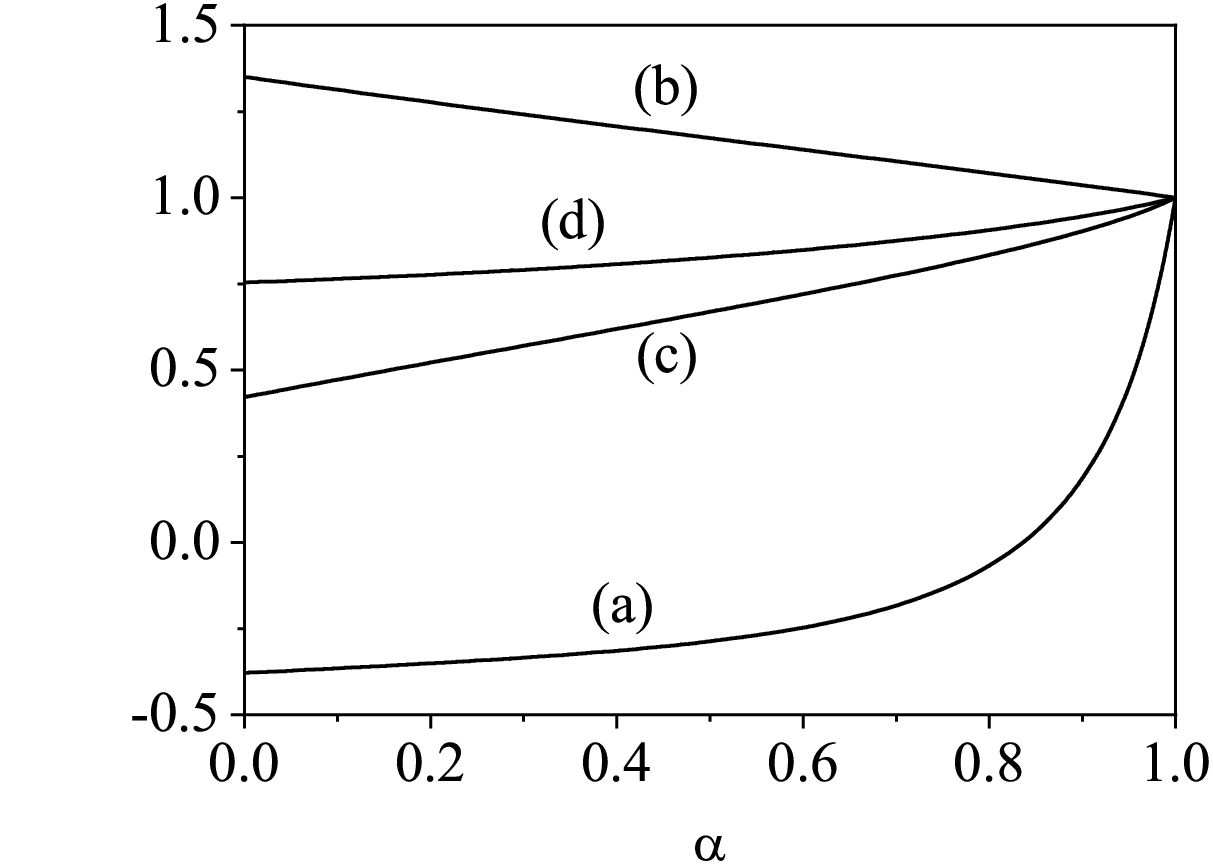
Refer to caption
Figure 3: Plot of the (reduced) diffusion coefficients D1T∗D_{1}^{T*} (a), D1U∗D_{1}^{U*} (b), D11∗D_{11}^{*} (c), and D12∗D_{12}^{*} (d) as a function of the common coefficient of restitution α\alpha for an equimolar mixture (x1=12x_{1}=\frac{1}{2}) of hard spheres (d=3d=3) with σ1/σ2=1\sigma_{1}/\sigma_{2}=1, m1/m2=4m_{1}/m_{2}=4, ϕ=0.2\phi=0.2, and Tex∗=0.1T_{\text{ex}}^{*}=0.1.

The results derived in Sec. VI for the diffusion transport coefficients, the shear and bulk viscosities and the first-order contributions to the partial temperatures and the cooling rate depend on the background temperature TexT_{\text{ex}}, the concentration x1x_{1}, the density or volume fraction ϕ\phi, and the mechanical parameters of the binary mixture (masses, diameters, and coefficients of restitution). As in our previous paper Khalil and Garzó 2013 on dilute granular suspensions, given that the new relevant feature is the dependence of the transport coefficients on inelasticity, we scale these coefficients with respect to their values for elastic collisions. Thus, the scaled transport coefficients depend on the parameter space: {Tex∗,x1,m1/m2,σ1/σ2,ϕ,α11,α22,α12}\left\{T_{\text{ex}}^{*},x_{1},m_{1}/m_{2},\sigma_{1}/\sigma_{2},\phi,\alpha_{11},\alpha_{22},\alpha_{12}\right\}. Moreover, for the sake of simplicity, the case of a common coefficient of restitution (α11=α22=α12≡α\alpha_{11}=\alpha_{22}=\alpha_{12}\equiv\alpha) of an equimolar hard-sphere mixture (x1=12x_{1}=\frac{1}{2} and d=3d=3) with a background temperature Tex∗=0.1T_{\text{ex}}^{*}=0.1 is considered. This reduces the parameter space to four quantities: {m1/m2,σ1/σ2,ϕ,α}\left\{m_{1}/m_{2},\sigma_{1}/\sigma_{2},\phi,\alpha\right\}.

To display the dependence of the transport coefficients on the coefficient of restitution, we have to provide the form for the pair distribution function χi​j(0)\chi_{ij}^{(0)}. In the case of spheres (d=3d=3), a good approximation of χi​j(0)\chi_{ij}^{(0)} is Boublik 1970; Grundke and Henderson 1972; Lee and Levesque 1973

χi​j=11−ϕ+32​ϕ(1−ϕ)2​σi​σj​M2σi​j​M3+12​ϕ2(1−ϕ)3​(σi​σj​M2σi​j​M3)2,\chi_{ij}=\frac{1}{1-\phi}+\frac{3}{2}\frac{\phi}{(1-\phi)^{2}}\frac{\sigma_{i}\sigma_{j}M_{2}}{\sigma_{ij}M_{3}}+\frac{1}{2}\frac{\phi^{2}}{(1-\phi)^{3}}\left(\frac{\sigma_{i}\sigma_{j}M_{2}}{\sigma_{ij}M_{3}}\right)^{2}, (116)

where Mℓ=∑ixi​σiℓM_{\ell}=\sum_{i}x_{i}\sigma_{i}^{\ell}. In addition, the functions RiR_{i} are defined by Eq. (11).

Refer to caption
Figure 4: Plot of the (reduced) shear viscosity coefficient η⁡(α)/η⁡(1)\eta(\alpha)/\eta(1) as a function of the common coefficient of restitution α\alpha for an equimolar mixture (x1=12x_{1}=\frac{1}{2}) of hard spheres (d=3d=3) with σ1/σ2=1\sigma_{1}/\sigma_{2}=1, ϕ=0.2\phi=0.2, and Tex∗=0.1T_{\text{ex}}^{*}=0.1. Two different values of the mass ratio are considered: m1/m2=0.5m_{1}/m_{2}=0.5 (a) and m1/m2=4m_{1}/m_{2}=4 (b).
Refer to caption
Figure 5: Plot of the (reduced) coefficient ϖ1∗\varpi_{1}^{*} as a function of the common coefficient of restitution α\alpha for an equimolar mixture (x1=12x_{1}=\frac{1}{2}) of hard spheres (d=3d=3) with σ1/σ2=1\sigma_{1}/\sigma_{2}=1, ϕ=0.2\phi=0.2, and Tex∗=0.1T_{\text{ex}}^{*}=0.1. Three different values of the mass ratio are considered: m1/m2=0.5m_{1}/m_{2}=0.5 (a), m1/m2=4m_{1}/m_{2}=4 (b), and m1/m2=10m_{1}/m_{2}=10 (c).
Refer to caption
Figure 6: Plot of the (reduced) bulk viscosity coefficient ηb​(α)/ηb​(1)\eta_{\text{b}}(\alpha)/\eta_{\text{b}}(1) as a function of the common coefficient of restitution α\alpha for an equimolar mixture (x1=12x_{1}=\frac{1}{2}) of hard spheres (d=3d=3) with σ1/σ2=1\sigma_{1}/\sigma_{2}=1, ϕ=0.2\phi=0.2, and Tex∗=0.1T_{\text{ex}}^{*}=0.1. Two different values of the mass ratio are considered: m1/m2=0.5m_{1}/m_{2}=0.5 (a) and m1/m2=10m_{1}/m_{2}=10 (b). The dashed lines are the results for the (reduced) bulk viscosity when the contribution ηb′′\eta_{\text{b}}^{\prime\prime} to ηb\eta_{\text{b}} is neglected.
Refer to caption
Figure 7: Plot of the magnitude of the (reduced) coefficient ζU\zeta_{U} as a function of the common coefficient of restitution α\alpha for an equimolar mixture (x1=12x_{1}=\frac{1}{2}) of hard spheres (d=3d=3) with σ1/σ2=1\sigma_{1}/\sigma_{2}=1, ϕ=0.2\phi=0.2, and Tex∗=0.1T_{\text{ex}}^{*}=0.1. Two different values of the mass ratio are considered: m1/m2=0.5m_{1}/m_{2}=0.5 (a) and m1/m2=10m_{1}/m_{2}=10 (b). The dashed lines are the results for the coefficient ζU\zeta_{U} when the contribution ζ(1,1)\zeta^{(1,1)} to ζU\zeta_{U} is neglected.

Figure 3 shows the α\alpha-dependence of the reduced diffusion coefficients Di​j∗D_{ij}^{*}, D1T∗D_{1}^{T*}, and D1U∗D_{1}^{U*} for m1/m2=4m_{1}/m_{2}=4, σ1/σ2=1\sigma_{1}/\sigma_{2}=1, and ϕ=0.1\phi=0.1. We recall that Di​j∗≡Di​j​(α)/Di​j​(1)D_{ij}^{*}\equiv D_{ij}(\alpha)/D_{ij}(1), D1T∗≡D1T(α)/D1T(1)D_{1}^{T*}\equiv D_{1}^{T}(\alpha)/D_{1}^{T}(1), and D1U∗≡D1U(α)/D1U(1)D_{1}^{U*}\equiv D_{1}^{U}(\alpha)/D_{1}^{U}(1), where Di​j​(1)D_{ij}(1), D1U​(1)D_{1}^{U}(1), and D1T​(1)D_{1}^{T}(1) are the values of the diffusion transport coefficients for elastic collisions. It is quite apparent first that the effect of inelasticity on diffusion coefficients is in general significant since the forms of the scaled coefficients Di​j∗D_{ij}^{*}, D1U∗D_{1}^{U*}, and D1T∗D_{1}^{T*} differs clearly from their elastic counterparts. This is specially relevant in the case of the thermal diffusion coefficient D1T∗D_{1}^{T*}. In addition, a comparison with the results obtained for dry granular mixtures (see for instance, Figs. 5.5, 5.6, and 5.7 of Ref. Garzó 2019 for the same mixture parameters) reveals significant differences between dry (no gas phase) and gas-solid flows when grains are mechanically different. Thus, while D11∗D_{11}^{*} and D12∗D_{12}^{*} increase with inelasticity for dry granular mixtures, the opposite happens for granular suspensions since they decrease as increasing inelasticity. The qualitative α\alpha-dependence of D1T∗D_{1}^{T*} is similar in both dry and gas-solid flows, although the influence of inelasticity on D1T∗D_{1}^{T*} is much more important in the latter case.

We consider now the (reduced) shear viscosity η∗≡η⁡(α)/η⁡(1)\eta^{*}\equiv\eta(\alpha)/\eta(1). Figure 4 shows η∗\eta^{*} versus α\alpha for σ1/σ2=1\sigma_{1}/\sigma_{2}=1, ϕ=0.2\phi=0.2, and two different values of the mass ratio. As with the diffusion coefficients, the effect of inelasticity on the shear viscosity is again significant since the inelasticity hinders the transport of momentum. Regarding the comparison with dry granular mixtures, we find qualitative differences since both theory Garzó and Dufty 1999b; Lutsko 2005; Garzó 2013; Murray et al. 2012 and simulations Garzó 2019; Montanero et al. 2005 have shown that while for relatively dilute dry granular gases η∗\eta^{*} increases with inelasticity, the opposite occurs for sufficiently dense granular mixtures. This non-monotonic behavior with density contrasts with the results obtained here for multicomponent granular suspensions since the scaled coefficient η∗\eta^{*} always decreases with increasing inelasticity regardless of the value of the solid volume fraction ϕ\phi. With respect to the influence of the mass ratio on the shear viscosity, we see that its impact on η∗\eta^{*} is relatively small. In particular, at a given value of α\alpha, η∗\eta^{*} decreases with decreasing the mass ratio m1/m2m_{1}/m_{2}.

An interesting quantity is the first-order contribution ϖ1\varpi_{1} to the partial temperature T1T_{1}. The reduced coefficient ϖ1∗≡(n​σ122​v0/T)​ϖ1\varpi_{1}^{*}\equiv(n\sigma_{12}^{2}v_{0}/T)\varpi_{1} is plotted in Fig. 6 as a function of α\alpha for σ1/σ2=1\sigma_{1}/\sigma_{2}=1, ϕ=0.2\phi=0.2, and three different values of the mass ratio. We observe that the influence of inelasticity on ϖ1∗\varpi_{1}^{*} is important, specially for high mass ratios. However, Fig. 6 highlights that the magnitude of ϖ1∗\varpi_{1}^{*} is much smaller than the other transport coefficients and hence, the impact of the first-order contribution T1(1)T_{1}^{(1)} on both the bulk viscosity ηb\eta_{\text{b}} (through the coefficient ηb′′\eta_{b}^{\prime\prime}) and the first-order contribution ζU\zeta_{U} (through the coefficient ζ(1,1)\zeta^{(1,1)}) to the cooling rate is expected to be small. This is confirmed by Figs. 6 and 7 for the reduced coefficients ηb​(α)/ηb​(1)\eta_{\text{b}}(\alpha)/\eta_{\text{b}}(1) and ζU\zeta_{U}, respectively. It is quite apparent that the theoretical predictions for the above coefficients with and without the contribution of ϖ1∗\varpi_{1}^{*} are practically identical, specially in the case of the bulk viscosity. As the shear viscosity coefficient, we also see that the bulk viscosity decreases with increasing inelasticity (independent of the mass ratio considered). Moreover, as for dry granular mixtures Gómez González and Garzó 2019b, the coefficient ζU\zeta_{U} is always negative and its magnitude increases with inelasticity.

In summary, the mass and momentum transport coefficients for a multicomponent granular suspension differ significantly from those for dry granular mixtures. In most of cases, the differences become greater with increasing inelasticity, and depending on the cases, there is a relevant influence of the mass ratio.

VIII Discussion

This paper has been focused on the determination of the Navier–Stokes transport coefficients of a binary granular suspension at moderate densities. The starting point of our study has been the set of Enskog kinetic equations for the velocity distribution functions fi​(𝐫,𝐯,t)f_{i}(\mathbf{r},\mathbf{v},t) of the solid particles. The effect of the gas phase on the solid particles has been accounted for by an effective force constituted by two terms, namely a viscous drag force proportional to the velocity of the particles and a stochastic Langevin-like term. Therefore, we have considered a simplified model where the effect of the interstitial gas on grains is explicitly accounted for but the state of the surrounding gas is assumed to be independent of the solid particles. On the other hand, this model is inspired in numerical and experimental results that can be found in the granular literature Yin and Sundaresan 2009b. This fact is reflected in the functional dependence of the friction coefficients γi\gamma_{i} on both the partial ϕi\phi_{i} and global ϕ=ϕ1+ϕ2\phi=\phi_{1}+\phi_{2} volume fractions, and the mechanical properties of grains (masses mim_{i} and diameters σi\sigma_{i}).

We have derived the Navier–Stokes hydrodynamic equations in two steps. First, the macroscopic balance equations (20)–(22) have been obtained from the Enskog equation (1). Particularly, these equations include terms that account for the impact of the gas phase on grains and the kinetic and collisional contributions to the fluxes are expressed as functionals of the velocity distribution functions fif_{i}. Second, the mass, momentum, and heat fluxes, together with the cooling rate appearing in the hydrodynamic equations have been evaluated by solving the Enskog equation by means of the Chapman–Enskog method up to first order in the spatial gradients. The constitutive equation for the mass flux is given by Eq. (78) where the diffusion coefficients DiTD_{i}^{T}, Di​jD_{ij}, and DiUD_{i}^{U} are defined by Eqs. (90)–(92), respectively. The pressure tensor is given by Eq. (87) where the bulk viscosity ηb\eta_{\text{b}} is defined by Eq. (99) and the shear viscosity η\eta is defined by Eqs. (95) (kinetic contribution) and (102) (collisional contribution). Finally, the constitutive equation for the heat flux is given by Eq. (88) where the kinetic contributions to the Dufour coefficients Dq,i​jD_{q,ij}, the thermal conductivity κ\kappa, and the velocity conductivity κU\kappa_{U} are given by Eqs. (96), (97), and (98), respectively. Within the context of small gradients, all the above results apply in principle to arbitrary degree of inelasticity and are not restricted to specific values of the parameters of the mixture. The present work extends to moderate densities a previous analysis carried out for dilute bidisperse granular suspensions Khalil and Garzó 2013; Khalil and Garzó 2019.

Before considering inhomogeneous situations, the homogeneous steady state has been studied. In this state, the distributions fi,sf_{i,s} adopt the form (43) where the scaled distributions φi,s\varphi_{i,s} depend on the steady temperature TsT_{s} through the dimensionless velocity 𝐜=𝐯/v0​(Ts)\mathbf{c}=\mathbf{v}/v_{0}(T_{s}) and the (scaled) temperature θ=Ts/Tex\theta=T_{s}/T_{\text{ex}}. This scaling differs from the one assumed for dry granular mixtures Garzó and Dufty 1999a where the temperature dependence of φi\varphi_{i} is only encoded through the dimensionless velocity 𝐜\mathbf{c}. Although the exact form of the distributions φi,s\varphi_{i,s} is not known, in order to estimate the partial temperatures Ti,s/TexT_{i,s}/T_{\text{ex}}, the distributions φi,s\varphi_{i,s} have been approximated by the Maxwellian distributions (47). This has allowed us to explicitly get the partial temperatures in terms of the parameters of the mixture. In spite of the crudeness of the above approximation, the theoretical predictions for T1,s/T2,sT_{1,s}/T_{2,s} agree well with MD simulations, specially for moderately dense systems. The goodness of the comparison supports the use of the Maxwellian approximation (47) in the evaluation of the transport coefficients. However, we find some discrepancies between theory and simulations that could be mitigated if one would consider the influence of the fourth cumulants on the distributions φi,s\varphi_{i,s}. We plan to calculate these cumulants in the near future and perform more simulations to assess the reliability of the Enskog theoretical predictions for homogeneous steady states.

Once the steady reference state is well characterized, the diffusion coefficients, the bulk and shear viscosities, and the first-order contributions to the partial temperatures and the cooling rate have been determined. As usual, in order to achieve explicit expressions for the above transport coefficients, the leading terms in a Sonine polynomial expansion have been considered. The explicit forms of the transport coefficients have been displayed along Sec. VI and the Appendix C: the coefficients D11D_{11} and D12D_{12} are the solutions of the algebraic equations (158), the coefficients D1UD_{1}^{U} and D1TD_{1}^{T} are given by Eqs. (108) and (166), respectively, the shear viscosity η\eta and the first-order coefficients ϖi\varpi_{i} are the solutions of Eqs. (168) and (C), respectively, and the first-order contribution ζU=ζ(1,0)+ζ(1,1)\zeta_{U}=\zeta^{(1,0)}+\zeta^{(1,1)} to the cooling rate is given by Eqs. (139), (113) and (114). An interesting point is that these coefficients are defined not only in terms of the hydrodynamic fields in the steady state but, in addition, there are contributions to the transport coefficients coming from the derivatives of the temperature ratio in the vicinity of the steady state. These contributions can be seen as a measure of the departure of the perturbed state from the steady reference state. The inclusion of the above derivatives introduces conceptual and practical difficulties not present in the case of dry granular mixtures Garzó et al. 2007a; Garzó et al. 2007b.

In reduced forms, the diffusion transport coefficients and the shear viscosity coefficient of the granular suspension exhibit a complex dependence on the parameter space of the problem. In particular, Fig. 3 highlights the significant impact of the gas phase on the mass transport since the α\alpha-dependence of the Navier–Stokes transport coefficients D1TD_{1}^{T}, D1UD_{1}^{U}, and Di​jD_{ij} is in general different from the one found in the case of dry granular mixtures Garzó 2019. Regarding the shear viscosity coefficient η\eta, a comparison with the dry granular results Garzó 2019 shows a qualitative agreement between dry and granular suspensions for not quite high densities although important quantitative differences are found. Apart from these coefficients, the first-order contributions ϖi\varpi_{i} to the partial temperatures TiT_{i} have been also computed. The evaluation of these coefficients is interesting by itself and also because they are involved in the calculation of both the bulk viscosity ηb\eta_{\text{b}} and the first-order contribution ζU\zeta_{U} to the cooling rate. The results obtained here show that the magnitude of ϖ1\varpi_{1} is in general very small (in fact, much smaller than the one recently found Gómez González and Garzó 2019b in the absence of gas phase) and hence, its impact on ηb\eta_{\text{b}} and ζU\zeta_{U} is very tiny [see Figs. 6 and 7]. This conclusion contrasts with recent findings for dry granular mixtures Gómez González and Garzó 2019b where the influence of ϖ1\varpi_{1} on both the bulk viscosity and the cooling rate must be taken into account for strong inelasticities and disparate masses.

In a subsequent paper, we plan to determine the heat flux transport coefficients and to perform a linear stability analysis of the homogeneous steady state as a possible application. In particular, given that the homogeneous steady state is stable in the dilute limit, we want to see if the density corrections to the transport coefficients can modify the stability of the above homogeneous state. In addition, it is also quite apparent that the reliability of the theoretical results derived here (which have been obtained under certain approximations) should be assessed against computer simulations. As happens for dry granular mixtures Brey et al. 2000; Montanero and Garzó 2003; Garzó and Montanero 2003; Garzó and Montanero 2004; Garzó and Vega Reyes 2009; Garzó and Vega Reyes 2012; Brey and Ruiz-Montero 2013; Mitrano et al. 2014, we expect that the present results stimulate the performance of appropriate simulations for bidisperse granular suspensions. In particular, we plan to undertake simulations to obtain the tracer diffusion coefficient (namely, a binary mixture where the concentration of one of the components is negligible) in a similar way as in the case of granular mixtures Brey et al. 2000; Garzó and Vega Reyes 2009; Garzó and Vega Reyes 2012. Moreover, we also plan to carry out simulations to measure the Navier–Stokes shear viscosity η\eta by studying the decay of a small perturbation to the transversal component of the velocity field Brey et al. 1999. Another possible project for the next future is to consider inelastic rough hard spheres in order to assess the impact of friction on the transport properties of the granular suspension. Studies along these lines will be worked out in the near future.

Acknowledgements.
The work of R.G.G. and V.G. has been supported by the Spanish Government through Grant No. FIS2016-76359-P and by the Junta de Extremadura (Spain) Grant Nos. IB16013 and GR18079, partially financed by “Fondo Europeo de Desarrollo Regional” funds. The research of R.G.G. has been also supported by the predoctoral fellowship BES-2017-079725 from the Spanish Government.

Appendix A Derivatives of the temperature ratio in the vicinity of the steady state

In this Appendix, the derivatives of the temperature ratio τ1=T1(0)/T\tau_{1}=T_{1}^{(0)}/T with respect to θ\theta, λ1\lambda_{1}, x1x_{1}, and ϕ\phi in the vicinity of the steady state are evaluated.

Let us consider first the derivative (∂τ1/∂θ)x1,λ1,ϕ(\partial\tau_{1}/\partial\theta)_{x_{1},\lambda_{1},\phi}. To get it, we consider Eq. (69) for i=1i=1:

Λ∗​θ​∂τ1∂θ=−τ1​Λ∗+Λ1∗,\Lambda^{*}\theta\frac{\partial\tau_{1}}{\partial\theta}=-\tau_{1}\Lambda^{*}+\Lambda_{1}^{*}, (117)

where Λ∗\Lambda^{*} and Λ1∗\Lambda_{1}^{*} are defined by Eqs. (70) and (71), respectively. According to Eq. (48), the (reduced) partial cooling rate ζ1,0∗\zeta_{1,0}^{*} can be written as

ζ1,0∗=τ11/2M1−1/2ζ1′(x1,β),\zeta_{1,0}^{*}=\tau_{1}^{1/2}M_{1}^{-1/2}\zeta_{1}^{\prime}(x_{1},\beta), (118)

where β=β1/β2=m1​τ2/(m2​τ1)\beta=\beta_{1}/\beta_{2}=m_{1}\tau_{2}/(m_{2}\tau_{1}), τ2=(1−x1​τ1)/x2\tau_{2}=(1-x_{1}\tau_{1})/x_{2}, and

ζ1′​(x1,β)\displaystyle\zeta_{1}^{\prime}(x_{1},\beta) =\displaystyle= 2​π(d−1)/2d​Γ​(d2)​x1​χ11(0)​(σ1σ12)d−1​(1−α112)\displaystyle\frac{\sqrt{2}\pi^{\left(d-1\right)/2}}{d\Gamma\left(\frac{d}{2}\right)}x_{1}\chi_{11}^{(0)}\left(\frac{\sigma_{1}}{\sigma_{12}}\right)^{d-1}\left(1-\alpha_{11}^{2}\right) (119)
+4​π(d−1)/2d​Γ​(d2)​x2​χ12(0)​μ21​(1+β)1/2​(1+α12)\displaystyle+\frac{4\pi^{\left(d-1\right)/2}}{d\Gamma\left(\frac{d}{2}\right)}x_{2}\chi_{12}^{(0)}\mu_{21}\left(1+\beta\right)^{1/2}\left(1+\alpha_{12}\right)
×[1−μ212​(1+α12)​(1+β)].\displaystyle\times\left[1-\frac{\mu_{21}}{2}\left(1+\alpha_{12}\right)\left(1+\beta\right)\right].

At the steady state, Λ∗=Λ1∗=Λ2∗=0\Lambda^{*}=\Lambda_{1}^{*}=\Lambda_{2}^{*}=0 and hence, according to Eq. (117), the derivative ∂τ1/∂θ\partial\tau_{1}/\partial\theta becomes indeterminate. On the other hand, as for dilute multicomponent granular suspensions Khalil and Garzó 2013, the above problem can be fixed by applying l’Hôpital’s rule. In this case, we take first the derivative with respect to θ\theta in both sides of Eq. (117) and then take the steady-state limit. After some algebra, one easily achieves the following quadratic equation for the derivative Δθ,1=(∂τ1/∂θ)s\Delta_{\theta,1}=\left(\partial\tau_{1}/\partial\theta\right)_{\text{s}}:

θ​Λ1(θ)​Δθ,12+(θ​Λ0(θ)+τ1​Λ1(θ)−Λ11(θ))​Δθ,1−Λ10(θ)\displaystyle\theta\Lambda_{1}^{(\theta)}\Delta_{\theta,1}^{2}+\left(\theta\Lambda_{0}^{(\theta)}+\tau_{1}\Lambda_{1}^{(\theta)}-\Lambda_{11}^{(\theta)}\right)\Delta_{\theta,1}-\Lambda_{10}^{(\theta)}
+τ1​Λ0(θ)=0,\displaystyle+\tau_{1}\Lambda_{0}^{(\theta)}=0, (120)

where Λ0(θ)=x1​Λ10(θ)+x2​Λ20(θ)\Lambda_{0}^{(\theta)}=x_{1}\Lambda_{10}^{(\theta)}+x_{2}\Lambda_{20}^{(\theta)} and Λ1(θ)=x1​Λ11(θ)+x2​Λ21(θ)\Lambda_{1}^{(\theta)}=x_{1}\Lambda_{11}^{(\theta)}+x_{2}\Lambda_{21}^{(\theta)}. Here, we have introduced the quantities

Λ10(θ)=γ1∗​θ−1​τ1−3​γ1∗​θ−2,Λ20(θ)=γ2∗​θ−1​τ2−3​γ2∗​θ−2,\Lambda_{10}^{(\theta)}=\gamma_{1}^{*}\theta^{-1}\tau_{1}-3\gamma_{1}^{*}\theta^{-2},\quad\Lambda_{20}^{(\theta)}=\gamma_{2}^{*}\theta^{-1}\tau_{2}-3\gamma_{2}^{*}\theta^{-2}, (121)
Λ11(θ)=−2γ1∗−32ζ10∗+τ1−1/2M11/2x2​M2(∂ζ1′∂β)x1,ϕ\Lambda_{11}^{(\theta)}=-2\gamma_{1}^{*}-\frac{3}{2}\zeta_{10}^{*}+\tau_{1}^{-1/2}\frac{M_{1}^{1/2}}{x_{2}M_{2}}\left(\frac{\partial\zeta^{\prime}_{1}}{\partial\beta}\right)_{x_{1},\phi} (122)
Λ21(θ)=2​x1x2​γ2∗+32​x1x2​ζ20∗+M1x2​M23/2​τ23/2τ12​(∂ζ2′∂β)x1,ϕ.\Lambda_{21}^{(\theta)}=2\frac{x_{1}}{x_{2}}\gamma_{2}^{*}+\frac{3}{2}\frac{x_{1}}{x_{2}}\zeta_{20}^{*}+\frac{M_{1}}{x_{2}M_{2}^{3/2}}\frac{\tau_{2}^{3/2}}{\tau_{1}^{2}}\left(\frac{\partial\zeta_{2}^{\prime}}{\partial\beta}\right)_{x_{1},\phi}. (123)

In Eqs. (A)–(123), although the subscript ss has been omitted for the sake of simplicity, it is understood that all the quantities are evaluated in the steady state. As for dilute driven granular mixtures Khalil and Garzó 2013, an analysis of the solutions to Eq. (A) shows that in general one of the roots leads to unphysical behavior of the diffusion coefficients. We take the other root as the physical root of the quadratic equation (A).

Once the derivative Δθ,1\Delta_{\theta,1} is known, we can determine the remaining derivatives in a similar way. In order to get (∂τ1/∂λ1)θ,x1,ϕ(\partial\tau_{1}/\partial\lambda_{1})_{\theta,x_{1},\phi}, we take first the derivative of Eq. (117) with respect to λ1\lambda_{1} and then consider the steady-state conditions. The final result is

Δλ1,1=−τ1​Λ0(λ1)−Λ10(λ1)+θ​Λ0(λ1)​Δθ,1θ​Λ1(θ)​Δθ,1+τ1​Λ1(θ)−Λ11(θ),\Delta_{\lambda_{1},1}=-\frac{\tau_{1}\Lambda_{0}^{(\lambda_{1})}-\Lambda_{10}^{(\lambda_{1})}+\theta\Lambda_{0}^{(\lambda_{1})}\Delta_{\theta,1}}{\theta\Lambda_{1}^{(\theta)}\Delta_{\theta,1}+\tau_{1}\Lambda_{1}^{(\theta)}-\Lambda_{11}^{(\theta)}}, (124)

where Λ0(λ)=x1​Λ10(λ1)+x2​Λ20(λ1)\Lambda_{0}^{(\lambda)}=x_{1}\Lambda_{10}^{(\lambda_{1})}+x_{2}\Lambda_{20}^{(\lambda_{1})}, and

Λ10(λ1)=2θ−1/2(θ−1−τ1),Λ20(λ)=2R2R1θ−1/2(θ−1−τ2).\Lambda_{10}^{(\lambda_{1})}=2\theta^{-1/2}\left(\theta^{-1}-\tau_{1}\right),\quad\Lambda_{20}^{(\lambda)}=2\frac{R_{2}}{R_{1}}\theta^{-1/2}\left(\theta^{-1}-\tau_{2}\right). (125)

Analogously, the derivative (∂τ1/∂x1)θ,λ1,ϕ(\partial\tau_{1}/\partial x_{1})_{\theta,\lambda_{1},\phi} in the steady state is

Δx1,1=−τ1​Λ0(x1)−Λ10(x1)+θ​Λ0(x1)​Δθ,1θ​Λ1(θ)​Δθ,1+τ1​Λ1(θ)−Λ11(θ),\Delta_{x_{1},1}=-\frac{\tau_{1}\Lambda_{0}^{(x_{1})}-\Lambda_{10}^{(x_{1})}+\theta\Lambda_{0}^{(x_{1})}\Delta_{\theta,1}}{\theta\Lambda_{1}^{(\theta)}\Delta_{\theta,1}+\tau_{1}\Lambda_{1}^{(\theta)}-\Lambda_{11}^{(\theta)}}, (126)

where Λ0(x1)=x1​Λ10(x1)+x2​Λ20(x1)\Lambda_{0}^{(x_{1})}=x_{1}\Lambda_{10}^{(x_{1})}+x_{2}\Lambda_{20}^{(x_{1})}, and

Λ10(x1)=−τ13/2M1−1/2(∂ζ1′∂x1)β,ϕ,\Lambda_{10}^{(x_{1})}=-\tau_{1}^{3/2}M_{1}^{-1/2}\bigg(\frac{\partial\zeta^{\prime}_{1}}{\partial x_{1}}\bigg)_{\beta,\phi}, (127)
Λ20(x1)\displaystyle\Lambda_{20}^{(x_{1})} =\displaystyle= 2​γ1∗x2​(θ−1−τ1)−2​γ2∗x2​(θ−1−τ2)\displaystyle 2\frac{\gamma_{1}^{*}}{x_{2}}\left(\theta^{-1}-\tau_{1}\right)-2\frac{\gamma_{2}^{*}}{x_{2}}\left(\theta^{-1}-\tau_{2}\right) (128)
−1−τ1x22​γ2∗+32​τ1−τ23x2​ζ2,0∗−τ1x2​ζ1,0∗\displaystyle-\frac{1-\tau_{1}}{x_{2}^{2}}\gamma_{2}^{*}+\frac{3}{2}\frac{\tau_{1}-\frac{\tau_{2}}{3}}{x_{2}}\zeta_{2,0}^{*}-\frac{\tau_{1}}{x_{2}}\zeta_{1,0}^{*}
−τ23/2M2−1/2(∂ζ2′∂x1)β,ϕ.\displaystyle-\tau_{2}^{3/2}M_{2}^{-1/2}\bigg(\frac{\partial\zeta^{\prime}_{2}}{\partial x_{1}}\bigg)_{\beta,\phi}.

Finally, in the steady state, the derivative (∂τ1/∂ϕ)θ,x1,λ1(\partial\tau_{1}/\partial\phi)_{\theta,x_{1},\lambda_{1}} is

Δϕ,1=−τ1​Λ0(ϕ)−Λ10(ϕ)+θ​Λ0(ϕ)​Δθ,1θ​Λ1(θ)​Δθ,1+τ1​Λ1(θ)−Λ11(θ),\Delta_{\phi,1}=-\frac{\tau_{1}\Lambda_{0}^{(\phi)}-\Lambda_{10}^{(\phi)}+\theta\Lambda_{0}^{(\phi)}\Delta_{\theta,1}}{\theta\Lambda_{1}^{(\theta)}\Delta_{\theta,1}+\tau_{1}\Lambda_{1}^{(\theta)}-\Lambda_{11}^{(\theta)}}, (129)

where Λ0(ϕ)=x1​Λ10(ϕ)+x2​Λ20(ϕ)\Lambda_{0}^{(\phi)}=x_{1}\Lambda_{10}^{(\phi)}+x_{2}\Lambda_{20}^{(\phi)}, and

Λ10(ϕ)=−τ13/2M1−1/2(∂ζ1′∂ϕ)x1,β,\Lambda_{10}^{(\phi)}=-\tau_{1}^{3/2}M_{1}^{-1/2}\bigg(\frac{\partial\zeta_{1}^{\prime}}{\partial\phi}\bigg)_{x_{1},\beta}, (130)
Λ20(ϕ)=−τ23/2M2−1/2(∂ζ2′∂ϕ)x1,β.\Lambda_{20}^{(\phi)}=-\tau_{2}^{3/2}M_{2}^{-1/2}\bigg(\frac{\partial\zeta_{2}^{\prime}}{\partial\phi}\bigg)_{x_{1},\beta}. (131)

Appendix B Some technical details on the first-order Chapman–Enskog solution

To first order in the spatial gradients, the distribution function fi(1)f_{i}^{(1)} obeys the Enskog kinetic equation

∂t(0)fi(1)−γi∂∂𝐯⋅𝐕fi(1)−γi​Texmi∂2fi(1)∂v2=−(Dt(1)+𝐕⋅∇)fi(0)+γiΔ𝐔⋅∂fi(0)∂𝐯−𝐠⋅∂fi(0)∂𝐯+∑j=12Ji​j(1)[fi,fj],\partial_{t}^{(0)}f_{i}^{(1)}-\gamma_{i}\frac{\partial}{\partial\mathbf{v}}\cdot\mathbf{V}f_{i}^{(1)}-\frac{\gamma_{i}T_{\text{ex}}}{m_{i}}\frac{\partial^{2}f_{i}^{(1)}}{\partial v^{2}}=-\left(D_{t}^{(1)}+\mathbf{V}\cdot\nabla\right)f_{i}^{(0)}+\gamma_{i}\Delta\mathbf{U}\cdot\frac{\partial f_{i}^{(0)}}{\partial\mathbf{v}}-\mathbf{g}\cdot\frac{\partial f_{i}^{(0)}}{\partial\mathbf{v}}+\sum_{j=1}^{2}\;J_{ij}^{(1)}[f_{i},f_{j}], (132)

where Dt(1)≡∂t(1)+𝐔⋅∇D_{t}^{(1)}\equiv\partial_{t}^{(1)}+\mathbf{U}\cdot\nabla and Ji​j(1)​[fi,fj]J_{ij}^{(1)}[f_{i},f_{j}] denotes the first-order contribution to the expansion of the Enskog collision operator in spatial gradients. To obtain Ji​j(1)​[fi,fj]J_{ij}^{(1)}[f_{i},f_{j}] one needs the expansions Garzó et al. 2007a; Garzó 2019

χi​j​(𝐫,𝐫±𝝈i​j|{nℓ})→∑ℓ=12χi​j(0)​(1±12​(nℓ​∂ln⁡χi​j(0)∂nℓ+Ii​j​ℓ)​𝝈i​j⋅∇ln⁡nℓ),\chi_{ij}\left(\mathbf{r},\mathbf{r}\pm\bm{\sigma}_{ij}|\left\{n_{\ell}\right\}\right)\rightarrow\sum_{\ell=1}^{2}\chi_{ij}^{(0)}\left(1\pm\frac{1}{2}\left(n_{\ell}\frac{\partial\ln\chi_{ij}^{(0)}}{\partial n_{\ell}}+I_{ij\ell}\right)\bm{\sigma}_{ij}\cdot\nabla\ln n_{\ell}\right), (133)
fj(0)(𝐫±𝝈i​j)→∑ℓ=12nℓ∂fj(0)∂nℓ𝝈i​j⋅∇lnnℓ−∂fj(0)∂Vβ(𝝈i​j⋅∇)Uβ+T∂fj(0)∂T𝝈i​j⋅∇lnT.f_{j}^{(0)}(\mathbf{r}\pm\bm{\sigma}_{ij})\rightarrow\sum_{\ell=1}^{2}n_{\ell}\frac{\partial f_{j}^{(0)}}{\partial n_{\ell}}\bm{\sigma}_{ij}\cdot\nabla\ln n_{\ell}-\frac{\partial f_{j}^{(0)}}{\partial V_{\beta}}(\bm{\sigma}_{ij}\cdot\nabla)U_{\beta}+T\frac{\partial f_{j}^{(0)}}{\partial T}\bm{\sigma}_{ij}\cdot\nabla\ln T. (134)

In Eq. (134), the quantities Ii​j​ℓI_{ij\ell} are defined in terms of the functional derivative of the (local) pair distribution function χi​j\chi_{ij} with respect to the (local) partial densities nℓn_{\ell}. These quantities are the origin of the primary difference between the so-called standard and revised Enskog kinetic theories for ordinary mixtures van Beijeren and Ernst 1973; López de Haro et al. 1983. The explicit forms of Ii​j​ℓI_{ij\ell} for a binary mixture of hard disks (d=2d=2) or spheres (d=3d=3) have been provided in the Appendix A of Ref. Garzó 2011b. Taking into account the expansions (133) and (134), the operator Ji​j(1)​[fi,fj]J_{ij}^{(1)}[f_{i},f_{j}] can be written as

∑j=12Ji​j(1)​[fi,fj]\displaystyle\sum_{j=1}^{2}J_{ij}^{(1)}[f_{i},f_{j}] →\displaystyle\rightarrow −∑j=12∑ℓ=12{𝓚i​j[nℓ∂fj(0)∂nℓ]+12(nℓ∂ln⁡χi​j(0)∂nℓ+Ii​j​ℓ)𝓚i​j[fj(0)]}⋅∇lnnℓ\displaystyle-\sum_{j=1}^{2}\sum_{\ell=1}^{2}\left\{\bm{\mathcal{K}}_{ij}\left[n_{\ell}\frac{\partial f_{j}^{(0)}}{\partial n_{\ell}}\right]+\frac{1}{2}\left(n_{\ell}\frac{\partial\ln\chi_{ij}^{(0)}}{\partial n_{\ell}}+I_{ij\ell}\right)\bm{\mathcal{K}}_{ij}\left[f_{j}^{(0)}\right]\right\}\cdot\nabla\ln n_{\ell} (135)
−∑j=12𝓚i​j[T∂fj(0)∂T]⋅∇lnT+12∑j=12𝒦i​j,λ[∂fj(0)∂Vβ](∂λUβ+∂βUλ−2dδλ​β∇⋅𝐔)\displaystyle-\sum_{j=1}^{2}\bm{\mathcal{K}}_{ij}\left[T\frac{\partial f_{j}^{(0)}}{\partial T}\right]\cdot\nabla\ln T+\frac{1}{2}\sum_{j=1}^{2}\mathcal{K}_{ij,\lambda}\left[\frac{\partial f_{j}^{(0)}}{\partial V_{\beta}}\right]\left(\partial_{\lambda}U_{\beta}+\partial_{\beta}U_{\lambda}-\frac{2}{d}\delta_{\lambda\beta}\nabla\cdot\mathbf{U}\right)
+1d∑j=12𝒦i​j,λ[∂fj(0)∂Vλ]∇⋅𝐔+∑j=12(Ji​j(0)[fi(1),fj(0)]+Ji​j(0)[fi(0),fj(1)]),\displaystyle+\frac{1}{d}\sum_{j=1}^{2}\mathcal{K}_{ij,\lambda}\left[\frac{\partial f_{j}^{(0)}}{\partial V_{\lambda}}\right]\nabla\cdot\mathbf{U}+\sum_{j=1}^{2}\left(J_{ij}^{(0)}\left[f_{i}^{(1)},f_{j}^{(0)}\right]+J_{ij}^{(0)}\left[f_{i}^{(0)},f_{j}^{(1)}\right]\right),

where the operator 𝓚i​j​[Xj]\bm{\mathcal{K}}_{ij}[X_{j}] is given by Garzó et al. 2007a; Garzó 2019

𝓚i​j​[Xj]=σi​jd​χi​j(0)​∫d​𝐯2​∫d​𝝈^​Θ​(𝝈^⋅𝐠12)​(𝝈^⋅𝐠12)​𝝈^​[αi​j−2​fi(0)​(𝐯1′′)​Xj​(𝐯2′′)+fi(0)​(𝐯1)​Xj​(𝐯2)].\bm{\mathcal{K}}_{ij}[X_{j}]=\sigma_{ij}^{d}\chi_{ij}^{(0)}\int\text{d}\mathbf{v}_{2}\int\text{d}\widehat{\bm{\sigma}}\Theta(\widehat{\bm{\sigma}}\cdot\mathbf{g}_{12})\left(\widehat{\bm{\sigma}}\cdot\mathbf{g}_{12}\right)\widehat{\bm{\sigma}}\left[\alpha_{ij}^{-2}f_{i}^{(0)}(\mathbf{v}_{1}^{\prime\prime})X_{j}(\mathbf{v}_{2}^{\prime\prime})+f_{i}^{(0)}(\mathbf{v}_{1})X_{j}(\mathbf{v}_{2})\right]. (136)

As for monocomponent granular suspensions Gómez González and Garzó 2019a, upon deriving Eq. (135) use has been made of the symmetry property 𝒦i​j,λ​[∂Vβfj(0)]=𝒦i​j,β​[∂Vλfj(0)]\mathcal{K}_{ij,\lambda}[\partial_{V_{\beta}}f_{j}^{(0)}]=\mathcal{K}_{ij,\beta}[\partial_{V_{\lambda}}f_{j}^{(0)}] that follows from the isotropy in velocity space of the zeroth-order distributions fi(0)f_{i}^{(0)}.

To first-order, the balance equations are

Dt(1)ni=−ni∇⋅𝐔,Dt(1)𝐔=−ρ−1∇p−Δ𝐔∑i=12ρiργi+𝐠+ρ−1(γ1−γ2)𝐣1(1),D_{t}^{(1)}n_{i}=-n_{i}\nabla\cdot\mathbf{U},\quad D_{t}^{(1)}\mathbf{U}=-\rho^{-1}\nabla p-\Delta\mathbf{U}\sum_{i=1}^{2}\frac{\rho_{i}}{\rho}\gamma_{i}+\mathbf{g}+\rho^{-1}\left(\gamma_{1}-\gamma_{2}\right)\mathbf{j}_{1}^{(1)}, (137)
Dt(1)T=−2​pd​n∇⋅𝐔−ζ(1)T−2∑i=12γixiTi(1).D_{t}^{(1)}T=-\frac{2p}{dn}\nabla\cdot\mathbf{U}-\zeta^{(1)}T-2\sum_{i=1}^{2}\gamma_{i}x_{i}T_{i}^{(1)}. (138)

Here, pp is given by Eq. (64) and ζ(1)\zeta^{(1)} is the first order contribution to the cooling rate. Since ζ(1)\zeta^{(1)} is a scalar, corrections to first-order in the gradients can arise only from ∇⋅𝐔\nabla\cdot\mathbf{U} since ∇ni\nabla n_{i} and ∇T\nabla T are vectors and the tensor ∂λUβ+∂βUλ−2dδλ​β∇⋅𝐔\partial_{\lambda}U_{\beta}+\partial_{\beta}U_{\lambda}-\frac{2}{d}\delta_{\lambda\beta}\nabla\cdot\mathbf{U} is a traceless tensor. Thus, ζ(1)=ζU∇⋅𝐔\zeta^{(1)}=\zeta_{U}\nabla\cdot\mathbf{U}, where ζU\zeta_{U} can be decomposed as ζU=ζ(1,0)+ζ(1,1)\zeta_{U}=\zeta^{(1,0)}+\zeta^{(1,1)}. The coefficient ζ(1,0)\zeta^{(1,0)} can be evaluated explicitly with the result Garzó et al. 2007b

ζ(1,0)=−3n​Tπd/2d2​Γ​(d2)∑i=12∑j=12ninjμj​iσi​jdχi​j(0)Ti(0)(1−αi​j2).\zeta^{(1,0)}=-\frac{3}{nT}\frac{\pi^{d/2}}{d^{2}\Gamma\left(\frac{d}{2}\right)}\sum_{i=1}^{2}\sum_{j=1}^{2}n_{i}n_{j}\mu_{ji}\sigma_{ij}^{d}\chi_{ij}^{(0)}T_{i}^{(0)}(1-\alpha_{ij}^{2}). (139)

On the other hand, the coefficient ζ(1,1)\zeta^{(1,1)} is given in terms of the first-order distributions fi(1)f_{i}^{(1)}. Its expression will be displayed latter. In addition, according to Eq. (64), ∇p\nabla p can be written as

∇p=∑i=12ni∂p∂ni∇lnni+p(1+θ∂ln⁡p∗∂θ)∇lnT,\nabla p=\sum_{i=1}^{2}n_{i}\frac{\partial p}{\partial n_{i}}\nabla\ln n_{i}+p\left(1+\theta\frac{\partial\ln p^{*}}{\partial\theta}\right)\nabla\ln T, (140)

where we recall that p∗=p/n​Tp^{*}=p/nT.

The right-hand side of Eq. (132) can be evaluated by using Eqs. (137)–(140) and the expansion (135) of the Enskog operator. With these results, the corresponding kinetic equation for fi(1)f_{i}^{(1)} reads

∂t(0)fi(1)−γi∂∂𝐯⋅𝐕fi(1)−γi​Texmi∂2fi(1)∂v2−(Tζ(1,1)+2∑j=12xjγjϖj)∂fi(0)∂T∇⋅𝐔−ρ−1(γ1−γ2)𝐣1(1)⋅∂fi(0)∂𝐕\displaystyle\partial_{t}^{(0)}f_{i}^{(1)}-\gamma_{i}\frac{\partial}{\partial\mathbf{v}}\cdot\mathbf{V}f_{i}^{(1)}-\frac{\gamma_{i}T_{\text{ex}}}{m_{i}}\frac{\partial^{2}f_{i}^{(1)}}{\partial v^{2}}-\left(T\zeta^{(1,1)}+2\sum_{j=1}^{2}x_{j}\gamma_{j}\varpi_{j}\right)\frac{\partial f_{i}^{(0)}}{\partial T}\nabla\cdot\mathbf{U}-\rho^{-1}\left(\gamma_{1}-\gamma_{2}\right)\mathbf{j}_{1}^{(1)}\cdot\frac{\partial f_{i}^{(0)}}{\partial\mathbf{V}}
−∑j=12(Ji​j(0)[fi(1),fj(0)]+Ji​j(0)[fi(0),fj(1)])=𝐀i⋅∇lnT+∑j=12𝐁i​j⋅∇lnnj+Ci,λ​β12(∂λUβ+∂βUλ−2dδλ​β∇⋅𝐔)\displaystyle-\sum_{j=1}^{2}\left(J_{ij}^{(0)}\left[f_{i}^{(1)},f_{j}^{(0)}\right]+J_{ij}^{(0)}\left[f_{i}^{(0)},f_{j}^{(1)}\right]\right)=\mathbf{A}_{i}\cdot\nabla\ln T+\sum_{j=1}^{2}\mathbf{B}_{ij}\cdot\nabla\ln n_{j}+C_{i,\lambda\beta}\frac{1}{2}\left(\partial_{\lambda}U_{\beta}+\partial_{\beta}U_{\lambda}-\frac{2}{d}\delta_{\lambda\beta}\nabla\cdot\mathbf{U}\right)
+Di∇⋅𝐔+𝐄i⋅Δ𝐔,\displaystyle+D_{i}\nabla\cdot\mathbf{U}+\mathbf{E}_{i}\cdot\Delta\mathbf{U}, (141)

where

𝐀i​(𝐕)=−𝐕​T​∂fi(0)∂T−pρ​(1+θ​∂ln⁡p∗∂θ)​∂fi(0)∂𝐕−∑j=12𝓚i​j​[T​∂fj(0)∂T],\mathbf{A}_{i}(\mathbf{V})=-\mathbf{V}T\frac{\partial f_{i}^{(0)}}{\partial T}-\frac{p}{\rho}\left(1+\theta\frac{\partial\ln p^{*}}{\partial\theta}\right)\frac{\partial f_{i}^{(0)}}{\partial\mathbf{V}}-\sum_{j=1}^{2}\bm{\mathcal{K}}_{ij}\left[T\frac{\partial f_{j}^{(0)}}{\partial T}\right], (142)
𝐁i​j​(𝐕)=−𝐕​nj​∂fi(0)∂nj−njρ​∂p∂nj​∂fi(0)∂𝐕−∑ℓ=12{𝓚i​ℓ​[nj​∂fℓ(0)∂nj]+12​(nj​∂ln⁡χi​ℓ(0)∂nj+Ii​ℓ​j)​𝓚i​ℓ​[fℓ(0)]},\mathbf{B}_{ij}(\mathbf{V})=-\mathbf{V}n_{j}\frac{\partial f_{i}^{(0)}}{\partial n_{j}}-\frac{n_{j}}{\rho}\frac{\partial p}{\partial n_{j}}\frac{\partial f^{(0)}_{i}}{\partial\mathbf{V}}-\sum_{\ell=1}^{2}\left\{\bm{\mathcal{K}}_{i\ell}\left[n_{j}\frac{\partial f_{\ell}^{(0)}}{\partial n_{j}}\right]+\frac{1}{2}\left(n_{j}\frac{\partial\ln\chi_{i\ell}^{(0)}}{\partial n_{j}}+I_{i\ell j}\right)\bm{\mathcal{K}}_{i\ell}\left[f_{\ell}^{(0)}\right]\right\}, (143)
Ci,β​λ​(𝐕)=Vλ​∂fi(0)∂Vβ+∑j=12𝒦i​j,λ​[∂fj(0)∂Vβ],C_{i,\beta\lambda}(\mathbf{V})=V_{\lambda}\frac{\partial f_{i}^{(0)}}{\partial V_{\beta}}+\sum_{j=1}^{2}\mathcal{K}_{ij,\lambda}\left[\frac{\partial f_{j}^{(0)}}{\partial V_{\beta}}\right], (144)
Di​(𝐕)=1d​∂∂𝐕⋅(𝐕​fi(0))+(ζ(1,0)+2d​p∗)​T​∂fi(0)∂T−fi(0)+∑j=12{nj​∂fi(0)∂nj+1d​𝒦i​j,λ​[∂fj(0)∂Vλ]},D_{i}(\mathbf{V})=\frac{1}{d}\frac{\partial}{\partial\mathbf{V}}\cdot\left(\mathbf{V}f_{i}^{(0)}\right)+\left(\zeta^{(1,0)}+\frac{2}{d}p^{*}\right)T\frac{\partial f_{i}^{(0)}}{\partial T}-f_{i}^{(0)}+\sum_{j=1}^{2}\left\{n_{j}\frac{\partial f^{(0)}_{i}}{\partial n_{j}}+\frac{1}{d}\mathcal{K}_{ij,\lambda}\left[\frac{\partial f_{j}^{(0)}}{\partial V_{\lambda}}\right]\right\}, (145)
𝐄i​(𝐕)=(γi−∑j=12ρjρ​γj)​∂fi(0)∂𝐕.\mathbf{E}_{i}\left(\mathbf{V}\right)=\left(\gamma_{i}-\sum_{j=1}^{2}\frac{\rho_{j}}{\rho}\gamma_{j}\right)\frac{\partial f^{(0)}_{i}}{\partial\mathbf{V}}. (146)

Note that in Eq. (B), ζ1(1)\zeta_{1}^{(1)} and ϖi\varpi_{i} are functionals of the first-order distributions fi(1)f_{i}^{(1)}. In Eq. (143), the derivative ∂fi(0)/∂nj\partial f_{i}^{(0)}/\partial n_{j} can be more explicitly written when one takes into account the scaling solution (43):

nj​∂fi(0)∂nj=δi​j​fj(0)+nj​fi(0)​(∂ln⁡φi∂x1​∂x1∂nj+∂ln⁡φi∂λ1​∂λ1∂nj+∂ln⁡φi∂ϕ​∂ϕ∂nj),n_{j}\frac{\partial f_{i}^{(0)}}{\partial n_{j}}=\delta_{ij}f_{j}^{(0)}+n_{j}f_{i}^{(0)}\left(\frac{\partial\ln\varphi_{i}}{\partial x_{1}}\frac{\partial x_{1}}{\partial n_{j}}+\frac{\partial\ln\varphi_{i}}{\partial\lambda_{1}}\frac{\partial\lambda_{1}}{\partial n_{j}}+\frac{\partial\ln\varphi_{i}}{\partial\phi}\frac{\partial\phi}{\partial n_{j}}\right), (147)

where

nj​∂x1∂nj=xj​(x2​δ1​j−x1​δ2​j),nj​∂ϕ∂nj=ϕj,n_{j}\frac{\partial x_{1}}{\partial n_{j}}=x_{j}\left(x_{2}\delta_{1j}-x_{1}\delta_{2j}\right),\quad n_{j}\frac{\partial\phi}{\partial n_{j}}=\phi_{j}, (148)
nj​∂λ1∂nj=λ1​(ϕj​∂ln⁡R1∂ϕ+∂ln⁡R1∂x1​nj​∂x1∂nj)−λ1​xj−λ1​ρjρ.n_{j}\frac{\partial\lambda_{1}}{\partial n_{j}}=\lambda_{1}\left(\phi_{j}\frac{\partial\ln R_{1}}{\partial\phi}+\frac{\partial\ln R_{1}}{\partial x_{1}}n_{j}\frac{\partial x_{1}}{\partial n_{j}}\right)-\lambda_{1}x_{j}-\lambda_{1}\frac{\rho_{j}}{\rho}. (149)

The solution to Eq. (B) is given by Eq. (IV.2). Because of the gradients ∇ni\nabla n_{i}, ∇T\nabla T, and ∇⋅𝐔\nabla\cdot\mathbf{U} as well as the traceless tensor ∂λUβ+∂βUλ−2dδλ​β∇⋅𝐔\partial_{\lambda}U_{\beta}+\partial_{\beta}U_{\lambda}-\frac{2}{d}\delta_{\lambda\beta}\nabla\cdot\mathbf{U} are all independents, substitution of the form (IV.2) into Eq. (B) leads to the following set of linear integral equations for the unknowns 𝓐i​(𝐕)\bm{\mathcal{A}}_{i}(\mathbf{V}), 𝓑i​j​(𝐕)\bm{\mathcal{B}}_{ij}(\mathbf{V}), 𝒞i,λ​β​(𝐕)\mathcal{C}_{i,\lambda\beta}(\mathbf{V}), and 𝒟i​(𝐕)\mathcal{D}_{i}(\mathbf{V}):

Λ(0)​T​∂T𝓐i−[2​∑j=12γj​xj​(θ−1+θ​∂τj∂θ)+12​ζ(0)+ζ(0)​θ​∂ln⁡ζ0∗∂θ]​𝓐i−γi​∂∂𝐯⋅𝐕​𝓐i−γi​Texmi​∂2∂v2​𝓐i\displaystyle\Lambda^{(0)}T\partial_{T}\bm{\mathcal{A}}_{i}-\left[2\sum_{j=1}^{2}\gamma_{j}x_{j}\left(\theta^{-1}+\theta\frac{\partial\tau_{j}}{\partial\theta}\right)+\frac{1}{2}\zeta^{(0)}+\zeta^{(0)}\theta\frac{\partial\ln\zeta_{0}^{*}}{\partial\theta}\right]\bm{\mathcal{A}}_{i}-\gamma_{i}\frac{\partial}{\partial\mathbf{v}}\cdot\mathbf{V}\bm{\mathcal{A}}_{i}-\frac{\gamma_{i}T_{\text{ex}}}{m_{i}}\frac{\partial^{2}}{\partial v^{2}}\bm{\mathcal{A}}_{i}
+(γ2−γ1)​D1T​∂fi(0)∂𝐕−∑j=12(Ji​j(0)​[𝓐i,fj(0)]+Ji​j(0)​[fi(0),𝓐j])=𝐀i,\displaystyle+\left(\gamma_{2}-\gamma_{1}\right)D_{1}^{T}\frac{\partial f_{i}^{(0)}}{\partial\mathbf{V}}-\sum_{j=1}^{2}\left(J_{ij}^{(0)}\left[\bm{\mathcal{A}}_{i},f_{j}^{(0)}\right]+J_{ij}^{(0)}\left[f_{i}^{(0)},\bm{\mathcal{A}}_{j}\right]\right)=\mathbf{A}_{i}, (150)
Λ(0)​T​∂T𝓑i​j−γi​∂∂𝐯⋅𝐕​𝓑i​j−γi​Texmi​∂2∂v2​𝓑i​j+(γ2−γ1)​m1​ρjρ2​D1​j​∂fi(0)∂𝐕−∑ℓ=12(Ji​ℓ(0)​[𝓑i​j,fℓ(0)]+Ji​ℓ(0)​[fi(0),𝓑ℓ​j])\displaystyle\Lambda^{(0)}T\partial_{T}\bm{\mathcal{B}}_{ij}-\gamma_{i}\frac{\partial}{\partial\mathbf{v}}\cdot\mathbf{V}\bm{\mathcal{B}}_{ij}-\frac{\gamma_{i}T_{\text{ex}}}{m_{i}}\frac{\partial^{2}}{\partial v^{2}}\bm{\mathcal{B}}_{ij}+\left(\gamma_{2}-\gamma_{1}\right)\frac{m_{1}\rho_{j}}{\rho^{2}}D_{1j}\frac{\partial f_{i}^{(0)}}{\partial\mathbf{V}}-\sum_{\ell=1}^{2}\left(J_{i\ell}^{(0)}\left[\bm{\mathcal{B}}_{ij},f_{\ell}^{(0)}\right]+J_{i\ell}^{(0)}\left[f_{i}^{(0)},\bm{\mathcal{B}}_{\ell j}\right]\right)
=𝐁i​j+[nj​∂ζ(0)∂nj−2​nj​∑ℓ=12{γℓ​xℓ​[(θ−1−τℓ)​(∂ln⁡γℓ∂nj+∂ln⁡xℓ∂nj)−(∂τℓ∂x1​∂x1∂nj+∂τℓ∂λ1​∂λ1∂nj+∂τℓ∂ϕ​∂ϕ∂nj)]}]​𝓐i,\displaystyle=\mathbf{B}_{ij}+\left[n_{j}\frac{\partial\zeta^{(0)}}{\partial n_{j}}-2n_{j}\sum_{\ell=1}^{2}\left\{\gamma_{\ell}x_{\ell}\left[\left(\theta^{-1}-\tau_{\ell}\right)\left(\frac{\partial\ln\gamma_{\ell}}{\partial n_{j}}+\frac{\partial\ln x_{\ell}}{\partial n_{j}}\right)-\left(\frac{\partial\tau_{\ell}}{\partial x_{1}}\frac{\partial x_{1}}{\partial n_{j}}+\frac{\partial\tau_{\ell}}{\partial\lambda_{1}}\frac{\partial\lambda_{1}}{\partial n_{j}}+\frac{\partial\tau_{\ell}}{\partial\phi}\frac{\partial\phi}{\partial n_{j}}\right)\right]\right\}\right]\bm{\mathcal{A}}_{i},
Λ(0)​T​∂T𝒞i,λ​β−γi​∂∂𝐯⋅𝐕​𝒞i,λ​β−γi​Texmi​∂2∂v2​𝒞i,λ​β−∑j=12(Ji​j(0)​[𝒞i,λ​β,fj(0)]+Ji​j(0)​[fi(0),𝒞j,λ​β])=Ci,λ​β,\Lambda^{(0)}T\partial_{T}\mathcal{C}_{i,\lambda\beta}-\gamma_{i}\frac{\partial}{\partial\mathbf{v}}\cdot\mathbf{V}\mathcal{C}_{i,\lambda\beta}-\frac{\gamma_{i}T_{\text{ex}}}{m_{i}}\frac{\partial^{2}}{\partial v^{2}}\mathcal{C}_{i,\lambda\beta}-\sum_{j=1}^{2}\left(J_{ij}^{(0)}\left[\mathcal{C}_{i,\lambda\beta},f_{j}^{(0)}\right]+J_{ij}^{(0)}\left[f_{i}^{(0)},\mathcal{C}_{j,\lambda\beta}\right]\right)=C_{i,\lambda\beta}, (152)
Λ(0)​T​∂T𝒟i−γi​∂∂𝐯⋅𝐕​𝒟i−γi​Texmi​∂2∂v2​𝒟i−(T​ζ(1,1)+2​∑j=12γj​xj​ϖj)​∂fi(0)∂T−∑j=12(Ji​j(0)​[𝒟i,fj(0)]+Ji​j(0)​[fi(0),𝒟j])=Di,\Lambda^{(0)}T\partial_{T}\mathcal{D}_{i}-\gamma_{i}\frac{\partial}{\partial\mathbf{v}}\cdot\mathbf{V}\mathcal{D}_{i}-\frac{\gamma_{i}T_{\text{ex}}}{m_{i}}\frac{\partial^{2}}{\partial v^{2}}\mathcal{D}_{i}-\left(T\zeta^{(1,1)}+2\sum_{j=1}^{2}\gamma_{j}x_{j}\varpi_{j}\right)\frac{\partial f_{i}^{(0)}}{\partial T}-\sum_{j=1}^{2}\left(J_{ij}^{(0)}\left[\mathcal{D}_{i},f_{j}^{(0)}\right]+J_{ij}^{(0)}\left[f_{i}^{(0)},\mathcal{D}_{j}\right]\right)=D_{i}, (153)
Λ(0)​T​∂T𝓔i−γi​∂∂𝐯⋅𝐕​𝓔i−γi​Texmi​∂2∂v2​𝓔i+ρ−1​(γ2−γ1)​D1U​∂fi(0)∂𝐕−∑j=12(Ji​j(0)​[𝓔i,fj(0)]+Ji​j(0)​[fi(0),𝓔j])=𝐄i,\Lambda^{(0)}T\partial_{T}\bm{\mathcal{E}}_{i}-\gamma_{i}\frac{\partial}{\partial\mathbf{v}}\cdot\mathbf{V}\bm{\mathcal{E}}_{i}-\frac{\gamma_{i}T_{\text{ex}}}{m_{i}}\frac{\partial^{2}}{\partial v^{2}}\bm{\mathcal{E}}_{i}+\rho^{-1}\left(\gamma_{2}-\gamma_{1}\right)D^{U}_{1}\frac{\partial f_{i}^{(0)}}{\partial\mathbf{V}}-\sum_{j=1}^{2}\left(J_{ij}^{(0)}\left[\bm{\mathcal{E}}_{i},f_{j}^{(0)}\right]+J_{ij}^{(0)}\left[f_{i}^{(0)},\bm{\mathcal{E}}_{j}\right]\right)=\mathbf{E}_{i}, (154)

where Λ(0)\Lambda^{(0)} is defined by Eq. (66). Upon deriving the above integral equations use has been made of the constitutive equation (78) for the mass flux 𝐣1(1)\mathbf{j}_{1}^{(1)} and the result

∂t(0)∇lnT=∇∂t(0)lnT=∇(2∑i=12γixi(θ−1−τi)−ζ(0))\displaystyle\partial_{t}^{(0)}\nabla\ln T=\nabla\partial_{t}^{(0)}\ln T=\nabla\bigg(2\sum_{i=1}^{2}\gamma_{i}x_{i}\left(\theta^{-1}-\tau_{i}\right)-\zeta^{(0)}\bigg) (155)
=\displaystyle= −∑j=12[nj∂ζ(0)∂nj−2nj∑ℓ=12{γℓxℓ[(θ−1−τℓ)(∂ln⁡γℓ∂nj+∂ln⁡xℓ∂nj)−(∂τℓ∂x1∂x1∂nj+∂τℓ∂λ1∂λ1∂nj+∂τℓ∂ϕ∂ϕ∂nj)]}]∇lnnj\displaystyle-\sum_{j=1}^{2}\left[n_{j}\frac{\partial\zeta^{(0)}}{\partial n_{j}}-2n_{j}\sum_{\ell=1}^{2}\left\{\gamma_{\ell}x_{\ell}\left[\left(\theta^{-1}-\tau_{\ell}\right)\left(\frac{\partial\ln\gamma_{\ell}}{\partial n_{j}}+\frac{\partial\ln x_{\ell}}{\partial n_{j}}\right)-\left(\frac{\partial\tau_{\ell}}{\partial x_{1}}\frac{\partial x_{1}}{\partial n_{j}}+\frac{\partial\tau_{\ell}}{\partial\lambda_{1}}\frac{\partial\lambda_{1}}{\partial n_{j}}+\frac{\partial\tau_{\ell}}{\partial\phi}\frac{\partial\phi}{\partial n_{j}}\right)\right]\right\}\right]\nabla\ln n_{j}
−[2∑i=12γixi(θ−1+θ∂τi∂θ)+12ζ(0)+ζ(0)θ∂ln⁡ζ0∗∂θ]∇lnT.\displaystyle-\left[2\sum_{i=1}^{2}\gamma_{i}x_{i}\left(\theta^{-1}+\theta\frac{\partial\tau_{i}}{\partial\theta}\right)+\frac{1}{2}\zeta^{(0)}+\zeta^{(0)}\theta\frac{\partial\ln\zeta_{0}^{*}}{\partial\theta}\right]\nabla\ln T.

Moreover, since ζ(1,1)\zeta^{(1,1)} is coupled to 𝒟i\mathcal{D}_{i}, its explicit form can be easily identified after expanding the expression (30) of the cooling rate to first order. The result is Garzó et al. 2007b

ζ(1,1)=1n​T​π(d−1)/2d​Γ​(d+32)​∑i=12∑j=12σi​jd−1​χi​j(0)​mi​j​(1−αi​j2)​∫d​𝐯1​∫d​𝐯2​g123​fi(0)​(𝐕1)​𝒟j​(𝐕2).\zeta^{(1,1)}=\frac{1}{nT}\frac{\pi^{(d-1)/2}}{d\Gamma\left(\frac{d+3}{2}\right)}\sum_{i=1}^{2}\sum_{j=1}^{2}\sigma_{ij}^{d-1}\chi_{ij}^{(0)}m_{ij}(1-\alpha_{ij}^{2})\int\text{d}\mathbf{v}_{1}\int\text{d}\mathbf{v}_{2}\;g_{12}^{3}\;f_{i}^{(0)}(\mathbf{V}_{1})\mathcal{D}_{j}(\mathbf{V}_{2}). (156)

The integral equations (IV.2)–(76) can be obtained from Eqs. (B)–(153) when the steady state condition (Λ(0)=0\Lambda^{(0)}=0) is assumed.

Appendix C Algebraic equations defining the transport coefficients

In this Appendix, we display the set of algebraic equations defining the diffusion transport coefficients, the shear viscosity coefficient, and the first-order contributions to the partial temperatures. In the case of the diffusion coefficients DiTD_{i}^{T}, Di​jD_{ij}, and DiUD_{i}^{U}, the set of algebraic equations are, respectively, given by

∑j=12{νi​j+(γ2−γ1)​ρiρ​δ1​j−[2​∑ℓ=12γℓ​xℓ​(θ−1−θ​Δθ,ℓ)+12​ζ(0)+ζ(0)​θ​∂ln⁡ζ0∗∂θ−γi]​δi​j}​DjT\displaystyle\sum_{j=1}^{2}\left\{\nu_{ij}+\left(\gamma_{2}-\gamma_{1}\right)\frac{\rho_{i}}{\rho}\delta_{1j}-\left[2\sum_{\ell=1}^{2}\gamma_{\ell}x_{\ell}\left(\theta^{-1}-\theta\Delta_{\theta,\ell}\right)+\frac{1}{2}\zeta^{(0)}+\zeta^{(0)}\theta\frac{\partial\ln\zeta_{0}^{*}}{\partial\theta}-\gamma_{i}\right]\delta_{ij}\right\}D_{j}^{T} (157)
=\displaystyle= −p​ρiρ2​(1+θ​∂ln⁡p∗∂θ−ρ​ni​Ti(0)p​ρi)+T​niρ​θ​Δθ,i+πd/2d​Γ​(d2)​ni​Tρ​∑j=12nj​μi​j​χi​j(0)​σi​jd​(1+αi​j)\displaystyle-\frac{p\rho_{i}}{\rho^{2}}\left(1+\theta\frac{\partial\ln p^{*}}{\partial\theta}-\frac{\rho n_{i}T_{i}^{(0)}}{p\rho_{i}}\right)+T\frac{n_{i}}{\rho}\theta\Delta_{\theta,i}+\frac{\pi^{d/2}}{d\Gamma\left(\frac{d}{2}\right)}\frac{n_{i}T}{\rho}\sum_{j=1}^{2}n_{j}\mu_{ij}\chi_{ij}^{(0)}\sigma_{ij}^{d}\left(1+\alpha_{ij}\right)
×(τj+θ​Δθ,j),\displaystyle\times\left(\tau_{j}+\theta\Delta_{\theta,j}\right),
∑ℓ=12[νi​ℓ+(γ2−γ1)​ρiρ​δ1​ℓ+γi​δi​ℓ]​mℓ​Dℓ​j=ρ​Tρj​{nj​τj​δi​j+n⁡[nj​∂x1∂nj​xi​Δx1,i+nj​∂λ1∂nj​xi​Δλ1,i+xi​ϕj​Δϕ,i]}\displaystyle\sum_{\ell=1}^{2}\left[\nu_{i\ell}+\left(\gamma_{2}-\gamma_{1}\right)\frac{\rho_{i}}{\rho}\delta_{1\ell}+\gamma_{i}\delta_{i\ell}\right]m_{\ell}D_{\ell j}=\frac{\rho T}{\rho_{j}}\Bigg\{n_{j}\tau_{j}\delta_{ij}+n\Bigg[n_{j}\frac{\partial x_{1}}{\partial n_{j}}x_{i}\Delta_{x_{1},i}+n_{j}\frac{\partial\lambda_{1}}{\partial n_{j}}x_{i}\Delta_{\lambda_{1},i}+x_{i}\phi_{j}\Delta_{\phi,i}\Bigg]\Bigg\} (158)
+\displaystyle+ ρ2mj​[∂ζ(0)∂nj−2​∑ℓ=12{γℓ​xℓ​[(θ−1−τℓ)​(∂ln⁡γℓ∂nj+∂ln⁡xℓ∂nj)−(∂x1∂nj​Δx1,ℓ+∂λ1∂nj​Δλ1,ℓ+ϕjnj​Δϕ,ℓ)]}]​DiT\displaystyle\frac{\rho^{2}}{m_{j}}\left[\frac{\partial\zeta^{(0)}}{\partial n_{j}}-2\sum_{\ell=1}^{2}\left\{\gamma_{\ell}x_{\ell}\left[\left(\theta^{-1}-\tau_{\ell}\right)\left(\frac{\partial\ln\gamma_{\ell}}{\partial n_{j}}+\frac{\partial\ln x_{\ell}}{\partial n_{j}}\right)-\left(\frac{\partial x_{1}}{\partial n_{j}}\Delta_{x_{1},\ell}+\frac{\partial\lambda_{1}}{\partial n_{j}}\Delta_{\lambda_{1},\ell}+\frac{\phi_{j}}{n_{j}}\Delta_{\phi,\ell}\right)\right]\right\}\right]D_{i}^{T}
−ρimj∂p∂nj+ρ​Tρjπd/2d​Γ​(d2)∑ℓ=12ninℓσi​ℓdχi​ℓ(0)mi​ℓ(1+αi​ℓ{[δj​ℓ+12(nj∂ln⁡χi​ℓ(0)∂nj+Ii​ℓ​j)](τimi+τℓmℓ)\displaystyle-\frac{\rho_{i}}{m_{j}}\frac{\partial p}{\partial n_{j}}+\frac{\rho T}{\rho_{j}}\frac{\pi^{d/2}}{d\Gamma\left(\frac{d}{2}\right)}\sum_{\ell=1}^{2}n_{i}n_{\ell}\sigma_{i\ell}^{d}\chi_{i\ell}^{(0)}m_{i\ell}(1+\alpha_{i\ell}\Bigg\{\Bigg[\delta_{j\ell}+\frac{1}{2}\left(n_{j}\frac{\partial\ln\chi_{i\ell}^{(0)}}{\partial n_{j}}+I_{i\ell j}\right)\Bigg]\Bigg(\frac{\tau_{i}}{m_{i}}+\frac{\tau_{\ell}}{m_{\ell}}\Bigg)
+njmℓ∂x1∂njΔx1,ℓ+njmℓ∂λ1∂njΔλ1,ℓ+ϕjmℓΔϕ,ℓ},\displaystyle+\frac{n_{j}}{m_{\ell}}\frac{\partial x_{1}}{\partial n_{j}}\Delta_{x_{1},\ell}+\frac{n_{j}}{m_{\ell}}\frac{\partial\lambda_{1}}{\partial n_{j}}\Delta_{\lambda_{1},\ell}+\frac{\phi_{j}}{m_{\ell}}\Delta_{\phi,\ell}\Bigg\},
∑j=12[νi​j+(γ2−γ1)​ρiρ​δ1​j+γi​δi​j]​DjU=ρi​(γi−∑j=12ρjρ​γj).\sum_{j=1}^{2}\left[\nu_{ij}+\left(\gamma_{2}-\gamma_{1}\right)\frac{\rho_{i}}{\rho}\delta_{1j}+\gamma_{i}\delta_{ij}\right]D^{U}_{j}=\rho_{i}\left(\gamma_{i}-\sum_{j=1}^{2}\frac{\rho_{j}}{\rho}\gamma_{j}\right). (159)

Here, the derivatives ∂x1/∂nj\partial x_{1}/\partial n_{j} and ∂λ1/∂nj\partial\lambda_{1}/\partial n_{j} are given by Eqs. (148) and (149), respectively, and the collision frequencies νi​j\nu_{ij} appearing in Eqs. (157)–(159) are defined as

νi​i=−mid​ni​Ti∫d𝐯𝐕⋅Ji​j(0)[fi,M𝐕,fj(0)],\nu_{ii}=-\frac{m_{i}}{dn_{i}T_{i}}\int\text{d}\mathbf{v}\;\mathbf{V}\cdot J_{ij}^{(0)}[f_{i,\text{M}}\mathbf{V},f_{j}^{(0)}], (160)
νi​j=−mid​nj​Tj∫d𝐯𝐕⋅Ji​j(0)[fi(0),fj,M𝐕],\nu_{ij}=-\frac{m_{i}}{dn_{j}T_{j}}\int\text{d}\mathbf{v}\;\mathbf{V}\cdot J_{ij}^{(0)}[f_{i}^{(0)},f_{j,\text{M}}\mathbf{V}], (161)

for i≠ji\neq j. Note that the self-collision terms of νi​i\nu_{ii} arising from Ji​i(0)​[fi​M​𝐕,fi(0)]J_{ii}^{(0)}[f_{i\text{M}}\mathbf{V},f_{i}^{(0)}] do not occur in Eq. (160) since they conserve momentum for the component ii. In addition, upon deriving Eqs. (157) and (158), use has been made of the results

∫d​𝐯​mi​𝐕⋅𝓚i​j​[T​∂fj(0)∂T]=πd/2Γ⁡(d2)​ni​nj​σi​jd​χi​j(0)​μi​j​(1+αi​j)​Tj(0)​(1+θτj​Δθ,j),\int\text{d}{\bf v}m_{i}\mathbf{V}\cdot\bm{\mathcal{K}}_{ij}\Bigg[T\frac{\partial f_{j}^{(0)}}{\partial T}\Bigg]=\frac{\pi^{d/2}}{\Gamma\left(\frac{d}{2}\right)}n_{i}n_{j}\sigma_{ij}^{d}\chi_{ij}^{(0)}\mu_{ij}(1+\alpha_{ij})T_{j}^{(0)}\left(1+\frac{\theta}{\tau_{j}}\Delta_{\theta,j}\right), (162)
∫d​𝐯​mi​𝐕⋅{𝓚i​ℓ​[nj​∂fℓ(0)∂nj]+12​(nj​∂ln⁡χi​ℓ(0)∂nj+Ii​ℓ​j)​𝓚i​ℓ​[fℓ(0)]}=πd/2Γ⁡(d2)​ni​T​nℓ​σi​ℓd​χi​ℓ(0)​mi​ℓ​(1+αi​ℓ)\displaystyle\int\text{d}{\bf v}m_{i}\mathbf{V}\cdot\left\{\bm{\mathcal{K}}_{i\ell}\left[n_{j}\frac{\partial f_{\ell}^{(0)}}{\partial n_{j}}\right]+\frac{1}{2}\left(n_{j}\frac{\partial\ln\chi_{i\ell}^{(0)}}{\partial n_{j}}+I_{i\ell j}\right)\bm{\mathcal{K}}_{i\ell}\left[f_{\ell}^{(0)}\right]\right\}=\frac{\pi^{d/2}}{\Gamma\left(\frac{d}{2}\right)}n_{i}Tn_{\ell}\sigma_{i\ell}^{d}\chi_{i\ell}^{(0)}m_{i\ell}(1+\alpha_{i\ell})
×{[δj​ℓ+12​(nj​∂ln⁡χi​ℓ(0)∂nj+Ii​ℓ​j)]​(τimi+τℓmℓ)+njmℓ​∂x1∂nj​Δx1,ℓ+njmℓ​∂λ1∂nj​Δλ1,ℓ+ϕjmℓ​Δϕ,ℓ},\displaystyle\times\Bigg\{\Bigg[\delta_{j\ell}+\frac{1}{2}\left(n_{j}\frac{\partial\ln\chi_{i\ell}^{(0)}}{\partial n_{j}}+I_{i\ell j}\right)\Bigg]\Bigg(\frac{\tau_{i}}{m_{i}}+\frac{\tau_{\ell}}{m_{\ell}}\Bigg)+\frac{n_{j}}{m_{\ell}}\frac{\partial x_{1}}{\partial n_{j}}\Delta_{x_{1},\ell}+\frac{n_{j}}{m_{\ell}}\frac{\partial\lambda_{1}}{\partial n_{j}}\Delta_{\lambda_{1},\ell}+\frac{\phi_{j}}{m_{\ell}}\Delta_{\phi,\ell}\Bigg\}, (163)

where fi(0)f_{i}^{(0)} has been replaced by fi,Mf_{i,\text{M}}. The explicit forms of the collision frequencies νi​i\nu_{ii} and νi​j\nu_{ij} can be also easily obtained by considering the latter replacement. They are given by Garzó and Montanero 2007

νi​i=2​π(d−1)/2d​Γ​(d2)​nj​σi​jd−1​χi​j(0)​μj​i​v0​(1+αi​j)​(βi+βjβi​βj)1/2,\nu_{ii}=\frac{2\pi^{(d-1)/2}}{d\Gamma\left(\frac{d}{2}\right)}n_{j}\sigma_{ij}^{d-1}\chi_{ij}^{(0)}\mu_{ji}v_{0}\left(1+\alpha_{ij}\right)\left(\frac{\beta_{i}+\beta_{j}}{\beta_{i}\beta_{j}}\right)^{1/2}, (164)
νi​j=−2​π(d−1)/2d​Γ​(d2)​ni​σi​jd−1​χi​j(0)​μi​j​v0​(1+αi​j)​(βi+βjβi​βj)1/2.\nu_{ij}=-\frac{2\pi^{(d-1)/2}}{d\Gamma\left(\frac{d}{2}\right)}n_{i}\sigma_{ij}^{d-1}\chi_{ij}^{(0)}\mu_{ij}v_{0}\left(1+\alpha_{ij}\right)\left(\frac{\beta_{i}+\beta_{j}}{\beta_{i}\beta_{j}}\right)^{1/2}. (165)

We recall that i≠ji\neq j in Eqs. (164) and (165). With these results, the explicit form of D1TD_{1}^{T} can be written as

D1T\displaystyle D_{1}^{T} =\displaystyle= [νD+ρ1​γ2+ρ2​γ1ρ−2∑j=12xjγj(θ−1−θΔθ,j)−ζ(0)(12+θ∂ln⁡ζ0∗∂θ)]−1{T​n1ρθΔθ,1\displaystyle\Bigg[\nu_{D}+\frac{\rho_{1}\gamma_{2}+\rho_{2}\gamma_{1}}{\rho}-2\sum_{j=1}^{2}x_{j}\gamma_{j}\left(\theta^{-1}-\theta\Delta_{\theta,j}\right)-\zeta^{(0)}\left(\frac{1}{2}+\theta\frac{\partial\ln\zeta_{0}^{*}}{\partial\theta}\right)\Bigg]^{-1}\Bigg\{\frac{Tn_{1}}{\rho}\theta\Delta_{\theta,1} (166)
−p​ρ1ρ2(1+θ∂ln⁡p∗∂θ−ρ​n1​T1(0)p​ρ1)+πd/2d​Γ​(d2)n1​Tρ[n12χ11(0)σ1d(1+α11)(τ1+θΔθ,1)\displaystyle-\frac{p\rho_{1}}{\rho^{2}}\left(1+\theta\frac{\partial\ln p^{*}}{\partial\theta}-\frac{\rho n_{1}T_{1}^{(0)}}{p\rho_{1}}\right)+\frac{\pi^{d/2}}{d\Gamma\left(\frac{d}{2}\right)}\frac{n_{1}T}{\rho}\Bigg[\frac{n_{1}}{2}\chi_{11}^{(0)}\sigma_{1}^{d}\left(1+\alpha_{11}\right)\left(\tau_{1}+\theta\Delta_{\theta,1}\right)
+n2μ12χ12(0)σ12d(1+α12)(τ2+θΔθ,2)]},\displaystyle+n_{2}\mu_{12}\chi_{12}^{(0)}\sigma_{12}^{d}\left(1+\alpha_{12}\right)\left(\tau_{2}+\theta\Delta_{\theta,2}\right)\Bigg]\Bigg\},

where νD\nu_{D} is

νD=ν11−ν12=2​π(d−1)/2d​Γ​(d2)​n​σ12d−1​χ12(0)​v0​(1+α12)​(β1+β2β1​β2)1/2​(x1​μ12+x2​μ21).\nu_{D}=\nu_{11}-\nu_{12}=\frac{2\pi^{(d-1)/2}}{d\Gamma\left(\frac{d}{2}\right)}n\sigma_{12}^{d-1}\chi_{12}^{(0)}v_{0}\left(1+\alpha_{12}\right)\left(\frac{\beta_{1}+\beta_{2}}{\beta_{1}\beta_{2}}\right)^{1/2}\left(x_{1}\mu_{12}+x_{2}\mu_{21}\right). (167)

We consider now the kinetic contribution ηk\eta_{\text{k}} to the shear viscosity coefficient η\eta. The kinetic coefficient ηk=η1k+η2k\eta_{\text{k}}=\eta_{1}^{\text{k}}+\eta_{2}^{\text{k}}, where the partial contributions ηik\eta_{i}^{\text{k}} (i=1,2)(i=1,2) obey the set of equations

∑j=12(τi​j+2​γi​δi​j)​ηjk=ni​Ti(0)+ρi​T​πd/2d⁡(d+2)​Γ​(d2)​∑j=12nj​μj​i​σi​jd​χi​j(0)​(1+αi​j)​[μj​i​(3​αi​j−1)​(τimi+τjmj)−4​τi−τjmi+mj],\sum_{j=1}^{2}\left(\tau_{ij}+2\gamma_{i}\delta_{ij}\right)\eta_{j}^{\text{k}}=n_{i}T^{(0)}_{i}+\frac{\rho_{i}T\pi^{d/2}}{d(d+2)\Gamma\left(\frac{d}{2}\right)}\sum_{j=1}^{2}n_{j}\mu_{ji}\sigma^{d}_{ij}\chi_{ij}^{(0)}\left(1+\alpha_{ij}\right)\Bigg[\mu_{ji}\left(3\alpha_{ij}-1\right)\left(\frac{\tau_{i}}{m_{i}}+\frac{\tau_{j}}{m_{j}}\right)-4\frac{\tau_{i}-\tau_{j}}{m_{i}+m_{j}}\Bigg], (168)

where the collision frequencies τi​j\tau_{ij} are defined as

τi​i=−1(d−1)​(d+2)​1ni​Ti(0)​2​(∫d​𝐯​Ri,λ​β​Ji​i(0)​[fi(0),fi​M​Ri,λ​β]+∑j=12∫d​𝐯​Ri,λ​β​Ji​j(0)​[fi,M​Ri,λ​β,fj(0)]),\tau_{ii}=-\frac{1}{(d-1)(d+2)}\frac{1}{n_{i}T_{i}^{(0)2}}\Bigg(\int\text{d}\mathbf{v}R_{i,\lambda\beta}J_{ii}^{(0)}\left[f_{i}^{(0)},f_{i\text{M}}R_{i,\lambda\beta}\right]+\sum_{j=1}^{2}\int\text{d}\mathbf{v}R_{i,\lambda\beta}J_{ij}^{(0)}\left[f_{i,\text{M}}R_{i,\lambda\beta},f_{j}^{(0)}\right]\Bigg), (169)
τi​j=−1(d−1)​(d+2)1nj​Tj(0)​2∫d𝐯Ri,λ​βJi​j(0)[fi(0),fj,MRj,λ​β],(i≠j).\tau_{ij}=-\frac{1}{(d-1)(d+2)}\frac{1}{n_{j}T_{j}^{(0)2}}\int\text{d}\mathbf{v}R_{i,\lambda\beta}J_{ij}^{(0)}\left[f_{i}^{(0)},f_{j,\text{M}}R_{j,\lambda\beta}\right],\quad(i\neq j). (170)

Upon deriving Eq. (168) use has been made of the result Garzó et al. 2007b

∫d​𝐯​Ri,λ​β​𝒦i​j,λ​[∂fj(0)∂Vβ]=−πd/2​(d−1)d​Γ​(d2)​ρi​nj​T​μj​i​σi​jd​χi​j(0)​(1+αi​j)​[μj​i​(3​αi​j−1)​(τimi+τjmj)−4​τi−τjmi+mj].\int\text{d}\mathbf{v}\;R_{i,\lambda\beta}\mathcal{K}_{ij,\lambda}\left[\frac{\partial f_{j}^{(0)}}{\partial V_{\beta}}\right]=-\frac{\pi^{d/2}(d-1)}{d\Gamma\left(\frac{d}{2}\right)}\rho_{i}n_{j}T\mu_{ji}\sigma^{d}_{ij}\chi_{ij}^{(0)}\left(1+\alpha_{ij}\right)\Bigg[\mu_{ji}\left(3\alpha_{ij}-1\right)\left(\frac{\tau_{i}}{m_{i}}+\frac{\tau_{j}}{m_{j}}\right)-4\frac{\tau_{i}-\tau_{j}}{m_{i}+m_{j}}\Bigg]. (171)

Explicit expressions of the collision frequencies τi​i\tau_{ii} and τi​j\tau_{ij} can be obtained by considering the Maxwellian approximation (103) to fi(0)f_{i}^{(0)}. The results are Garzó et al. 2007b

τi​i\displaystyle\tau_{ii} =\displaystyle= 2​π(d−1)/2d⁡(d+2)​Γ​(d2)v0{niσid−1χi​i(0)(2βi)−1/2(3+2d−3αi​i)(1+αi​i)+2njχi​j(0)σi​jd−1μj​i(1+αi​j)βi3/2βj−1/2\displaystyle\frac{2\pi^{(d-1)/2}}{d(d+2)\Gamma\left(\frac{d}{2}\right)}v_{0}\Bigg\{n_{i}\sigma_{i}^{d-1}\chi_{ii}^{(0)}\left(2\beta_{i}\right)^{-1/2}\left(3+2d-3\alpha_{ii}\right)\left(1+\alpha_{ii}\right)+2n_{j}\chi_{ij}^{(0)}\sigma_{ij}^{d-1}\mu_{ji}\left(1+\alpha_{ij}\right)\beta_{i}^{3/2}\beta_{j}^{-1/2}
×[(d+3)βi​jβi−2(βi+βj)−1/2+3+2​d−3​αi​j2μj​iβi−2(βi+βj)1/2+2​d​(d−1)−42​(d−1)βi−1(βi+βj)−1/2]},\displaystyle\times\Bigg[\left(d+3\right)\beta_{ij}\beta_{i}^{-2}\left(\beta_{i}+\beta_{j}\right)^{-1/2}+\frac{3+2d-3\alpha_{ij}}{2}\mu_{ji}\beta_{i}^{-2}\left(\beta_{i}+\beta_{j}\right)^{1/2}+\frac{2d(d-1)-4}{2(d-1)}\beta_{i}^{-1}\left(\beta_{i}+\beta_{j}\right)^{-1/2}\Bigg]\Bigg\},
τi​j\displaystyle\tau_{ij} =\displaystyle= 4​π(d−1)/2d⁡(d+2)​Γ​(d2)v0niχi​j(0)σi​jd−1μi​jβj3/2βi−1/2(1+αi​j)[(d+3)βi​jβj−2(βi+βj)−1/2+3+2​d−3​αi​j2\displaystyle\frac{4\pi^{(d-1)/2}}{d(d+2)\Gamma\left(\frac{d}{2}\right)}v_{0}n_{i}\chi_{ij}^{(0)}\sigma_{ij}^{d-1}\mu_{ij}\beta_{j}^{3/2}\beta_{i}^{-1/2}\left(1+\alpha_{ij}\right)\Bigg[\left(d+3\right)\beta_{ij}\beta_{j}^{-2}\left(\beta_{i}+\beta_{j}\right)^{-1/2}+\frac{3+2d-3\alpha_{ij}}{2} (173)
×μj​iβj−2(βi+βj)1/2−2​d​(d+1)−42​(d−1)βj−1(βi+βj)−1/2],\displaystyle\times\mu_{ji}\beta_{j}^{-2}\left(\beta_{i}+\beta_{j}\right)^{1/2}-\frac{2d(d+1)-4}{2(d-1)}\beta_{j}^{-1}\left(\beta_{i}+\beta_{j}\right)^{-1/2}\Bigg],

where βi​j=μi​j​βj−μj​i​βi\beta_{ij}=\mu_{ij}\beta_{j}-\mu_{ji}\beta_{i} and i≠ji\neq j.

Finally, the first-order contributions Ti(1)T_{i}^{(1)} to the partial temperatures are defined as Ti(1)=ϖi∇⋅𝐔T_{i}^{(1)}=\varpi_{i}\nabla\cdot\mathbf{U}. The set of algebraic equations defining the coefficients ϖi\varpi_{i} are given by

∑j=12[ωi​j+2​γj​xj​(τi+θ​Δθ,i)−2​γi​δi​j+(Ti(0)+T​θ​Δθ,i)​ξj]​ϖj=2d​Ti(0)−(ζ(1,0)+2d​p∗)​(Ti(0)+T​θ​Δθ,i)\displaystyle\sum_{j=1}^{2}\Big[\omega_{ij}+2\gamma_{j}x_{j}\left(\tau_{i}+\theta\Delta_{\theta,i}\right)-2\gamma_{i}\delta_{ij}+\left(T_{i}^{(0)}+T\theta\Delta_{\theta,i}\right)\xi_{j}\Big]\varpi_{j}=\frac{2}{d}T_{i}^{(0)}-\left(\zeta^{(1,0)}+\frac{2}{d}p^{*}\right)\left(T_{i}^{(0)}+T\theta\Delta_{\theta,i}\right)
+T∑j=12{πd/2d2​Γ​(d2)njσi​jdχi​j(0)mi​j(1+αi​j)[3μj​i(1+αi​j)(τimi+τjmj)−4τimi]−nj(∂λ1∂njΔλ1,i+∂ϕ∂njΔϕ,i)},\displaystyle+T\sum_{j=1}^{2}\Bigg\{\frac{\pi^{d/2}}{d^{2}\Gamma\left(\frac{d}{2}\right)}n_{j}\sigma_{ij}^{d}\chi_{ij}^{(0)}m_{ij}(1+\alpha_{ij})\left[3\mu_{ji}\left(1+\alpha_{ij}\right)\left(\frac{\tau_{i}}{m_{i}}+\frac{\tau_{j}}{m_{j}}\right)-4\frac{\tau_{i}}{m_{i}}\right]-n_{j}\left(\frac{\partial\lambda_{1}}{\partial n_{j}}\Delta_{\lambda_{1},i}+\frac{\partial\phi}{\partial n_{j}}\Delta_{\phi,i}\right)\Bigg\},

where ζ(1,0)\zeta^{(1,0)} is defined by Eq. (139) and the collision frequencies ωi​j\omega_{ij} are

ωi​i=1d​ni​Ti(0)​(∑j=12∫d​𝐯​mi​V2​Ji​j(0)​[fi,M​Wi,fj(0)]+∫d​𝐯​mi​V2​Ji​i(0)​[fi(0),fi​M​Wi]),\omega_{ii}=\frac{1}{dn_{i}T_{i}^{(0)}}\Bigg(\sum_{j=1}^{2}\int\text{d}\mathbf{v}m_{i}V^{2}J_{ij}^{(0)}\left[f_{i,\text{M}}W_{i},f_{j}^{(0)}\right]+\int\text{d}\mathbf{v}m_{i}V^{2}J_{ii}^{(0)}\left[f_{i}^{(0)},f_{i\text{M}}W_{i}\right]\Bigg), (175)
ωi​j=1d​ni​Tj(0)​∫d​𝐯​mi​V2​Ji​j(0)​[fi(0),fj,M​Wj],(i≠j).\omega_{ij}=\frac{1}{dn_{i}T_{j}^{(0)}}\int\text{d}\mathbf{v}m_{i}V^{2}J_{ij}^{(0)}\left[f_{i}^{(0)},f_{j,\text{M}}W_{j}\right],\quad(i\neq j). (176)

Upon deriving Eq. (C), we have accounted for that ∑jnj​∂njx1=0\sum_{j}n_{j}\partial_{n_{j}}x_{1}=0 and use has been made of the result Gómez González and Garzó 2019b

∫d​𝐯​mi​V2​𝒦i​j,λ​[∂fj(0)∂Vλ]=−πd/2Γ⁡(d2)​χi​j(0)​ni​nj​σi​jd​(1+αi​j)​[3​μj​i​(1+αi​j)​(Ti(0)mi+Tj(0)mi)−4​Ti(0)mi].\int\text{d}\mathbf{v}m_{i}V^{2}\mathcal{K}_{ij,\lambda}\left[\frac{\partial f_{j}^{(0)}}{\partial V_{\lambda}}\right]=-\frac{\pi^{d/2}}{\Gamma\left(\frac{d}{2}\right)}\chi_{ij}^{(0)}n_{i}n_{j}\sigma_{ij}^{d}(1+\alpha_{ij})\Bigg[3\mu_{ji}(1+\alpha_{ij})\left(\frac{T_{i}^{(0)}}{m_{i}}+\frac{T_{j}^{(0)}}{m_{i}}\right)-4\frac{T_{i}^{(0)}}{m_{i}}\Bigg]. (177)

Moreover, in the Maxwellian approximation (103), the collision frequencies ωi​i\omega_{ii} and ωi​j\omega_{ij} read Gómez González and Garzó 2019c

ωi​i\displaystyle\omega_{ii} =\displaystyle= −π(d−1)/22​d​Ti(0)​Γ​(d2)v03{32niσid−1miχi​i(0)βi−3/2(1−αi​i2)−njmi​jσi​jd−1χi​j(0)(1+αi​j)\displaystyle-\frac{\pi^{(d-1)/2}}{2dT_{i}^{(0)}\Gamma\left(\frac{d}{2}\right)}v_{0}^{3}\Bigg\{\frac{3}{\sqrt{2}}n_{i}\sigma_{i}^{d-1}m_{i}\chi_{ii}^{(0)}\beta_{i}^{-3/2}\left(1-\alpha_{ii}^{2}\right)-n_{j}m_{ij}\sigma_{ij}^{d-1}\chi_{ij}^{(0)}\left(1+\alpha_{ij}\right) (178)
×(βi+βj)−1/2βi−3/2βj−1/2[3μj​i(1+αi​j)(βi+βj)−2(2βi+3βj)]},\displaystyle\times\left(\beta_{i}+\beta_{j}\right)^{-1/2}\beta_{i}^{-3/2}\beta_{j}^{-1/2}\Big[3\mu_{ji}\left(1+\alpha_{ij}\right)\left(\beta_{i}+\beta_{j}\right)-2\left(2\beta_{i}+3\beta_{j}\right)\Big]\Bigg\},
ωi​j=π(d−1)/22​d​Tj(0)​Γ​(d2)v03njmi​jσi​jd−1χi​j(0)(1+αi​j)(βi+βj)−1/2βi−1/2βj−3/2[3μj​i(1+αi​j)(βi+βj)−2βj].\omega_{ij}=\frac{\pi^{(d-1)/2}}{2dT_{j}^{(0)}\Gamma\left(\frac{d}{2}\right)}v_{0}^{3}n_{j}m_{ij}\sigma_{ij}^{d-1}\chi_{ij}^{(0)}\left(1+\alpha_{ij}\right)\left(\beta_{i}+\beta_{j}\right)^{-1/2}\beta_{i}^{-1/2}\beta_{j}^{-3/2}\Big[3\mu_{ji}\left(1+\alpha_{ij}\right)\left(\beta_{i}+\beta_{j}\right)-2\beta_{j}\Big]. (179)

In Eqs. (178)–(179), it is understood that i≠ji\neq j.

References

  • Möbius et al. (2001) M. E. Möbius, B. E. Lauderdale, S. R. Nagel, and H. M. Jaeger, “Brazil-nut effect: Size separation of granular particles,” Nature 414, 270 (2001).
  • Naylor et al. (2003) M. A. Naylor, M. R. Swift, and P. J. King, “Air-driven Brazil nut effect,” Phys. Rev. E 68, 012301 (2003).
  • Sánchez et al. (2004) P. Sánchez, M. R. Swift, and P. J. King, “Stripe formation in granular mixtures due to the differential influence of drag,” Phys. Rev. Lett. 93, 184302 (2004).
  • Wylie et al. (2008) J. J. Wylie, Q. Zhang, H. Y. Xu, and X. X. Sun, “Drag-induced particle segregation with vibrating boundaries,” Europhys. Lett. 81, 54001 (2008).
  • Clement et al. (2010) C. P. Clement, H. A. Pacheco-Martínez, M. R. Swift, and P. J. King, “The water-enhanced Brazil nut effect,” Europhys. Lett. 91, 54001 (2010).
  • Pastenes et al. (2014) J. C. Pastenes, J. C. Géminard, and F. Melo, “Interstitial gas effect on vibrated granular columns,” Phy. Rev. E 89, 062205 (2014).
  • Koch and Hill (2001) D. L. Koch and R. J. Hill, “Inertial effects in suspensions and porous-media flows,” Annu. Rev. Fluid Mech. 33, 619–647 (2001).
  • Gradenigo et al. (2011) G. Gradenigo, A. Sarracino, D. Villamaina, and A. Puglisi, “Fluctuating hydrodynamics and correlation lengths in a driven granular fluid,” J. Stat. Mech. P08017 (2011).
  • Garzó et al. (2012) V. Garzó, S. Tenneti, S. Subramaniam, and C. M. Hrenya, “Enskog kinetic theory for monodisperse gas-solid flows,” J. Fluid Mech. 712, 129–168 (2012).
  • Khalil and Garzó (2013) N. Khalil and V. Garzó, “Transport coefficients for driven granular mixtures at low-density,” Phys. Rev. E 88, 052201 (2013).
  • Hayakawa et al. (2017) H. Hayakawa, S. Takada, and V. Garzó, “Kinetic theory of shear thickening for a moderately dense gas-solid suspension: From discontinuous thickening to continuous thickening,” Phys. Rev. E 96, 042903 (2017).
  • van Kampen (1981) N. G. van Kampen, Stochastic Processes in Physics and Chemistry (North Holland, Amsterdam, 1981).
  • Williams and MacKintosh (1996) D. R. M. Williams and F. C. MacKintosh, “Driven granular media in one dimension: Correlations and equation of state,” Phys. Rev. E 54, R9–R12 (1996).
  • Gómez González and Garzó (2019a) R. Gómez González and V. Garzó, “Transport coefficients for granular suspensions at moderate densities,” J. Stat. Mech. 093204 (2019a).
  • Chapman and Cowling (1970) S. Chapman and T. G. Cowling, The Mathematical Theory of Nonuniform Gases (Cambridge University Press, Cambridge, 1970).
  • Khalil and Garzó (2018) N Khalil and V Garzó, “Heat flux of driven granular mixtures at low density: Stability analysis of the homogeneous steady state,” Phys. Rev. E 97, 022902 (2018).
  • Khalil and Garzó (2019) N Khalil and V. Garzó, “Erratum: Transport coefficients for driven granular mixtures at low density [Phys. Rev. E 88, 052201 (2013)] and Heat flux of driven granular mixtures at low density: Stability analysis of the homogeneous steady state [Phys. Rev. E 97, 022902 (2018)],” Phys. Rev. E 99, 059901 (E) (2019).
  • Garzó (2019) V. Garzó, Granular Gaseous Flows (Springer Nature Switzerland, Basel, 2019).
  • Garzó and Montanero (2002) V. Garzó and J. M. Montanero, “Transport coefficients of a heated granular gas,” Physica A 313, 336–356 (2002).
  • Garzó (2011a) V. Garzó, “Transport coefficients of driven granular fluids at moderate volume fractions,” Phys. Rev. E 84, 012301 (2011a).
  • Gómez González and Garzó (2019b) R. Gómez González and V. Garzó, “Influence of the first-order contributions to the partial temperatures on transport properties in polydisperse dense granular mixtures,” Phys. Rev. E 100, 032904 (2019b).
  • Garzó et al. (2007a) V. Garzó, J. W. Dufty, and C. M. Hrenya, “Enskog theory for polydisperse granular mixtures. I. Navier–Stokes order transport,” Phys. Rev. E 76, 031303 (2007a).
  • Garzó et al. (2007b) V. Garzó, C. M. Hrenya, and J. W. Dufty, “Enskog theory for polydisperse granular mixtures. II. Sonine polynomial approximation,” Phys. Rev. E 76, 031304 (2007b).
  • Murray et al. (2012) J. A. Murray, V. Garzó, and C. M. Hrenya, “Enskog theory for polydisperse granular mixtures. III. Comparison of dense and dilute transport coefficients and equations of state for a binary mixture,” Powder Technol. 220, 24–36 (2012).
  • García de Soria et al. (2012) M. I. García de Soria, P. Maynar, and E. Trizac, “Universal reference state in a driven homogeneous granular gas,” Phys. Rev. E 85, 051301 (2012).
  • Chamorro et al. (2013) M. G. Chamorro, F. Vega Reyes, and V. Garzó, “Homogeneous steady states in a granular fluid driven by a stochastic bath with friction,” J. Stat. Mech. P07013 (2013).
  • Gómez González and Garzó (2019c) R. Gómez González and V. Garzó, “Simple shear flow in granular suspensiones: Inelastic Maxwell models and BGK-type kinetic model,” J. Stat. Mech. 013206 (2019c).
  • Yin and Sundaresan (2009a) X. Yin and S. Sundaresan, “Drag law for bidisperse gas-solid suspensions containing equally sized spheres,” Ind. Eng. Chem. Res. 48, 227–241 (2009a).
  • Yin and Sundaresan (2009b) X. Yin and S. Sundaresan, “Fluid-particle drag in low-Reynolds-number polydisperse gas-solid suspensions,” AIChE 55, 1352–1368 (2009b).
  • Holloway et al. (2010) W. Holloway, X. Yin, and S. Sundaresan, “Fluid-particle drag in inertial polydisperse gas-solid suspensions,” AIChE 56, 1995–2004 (2010).
  • van Noije and Ernst (1998) T. P. C. van Noije and M. H. Ernst, “Velocity distributions in homogeneous granular fluids: the free and heated case,” Granular Matter 1, 57–64 (1998).
  • Henrique et al. (2000) C. Henrique, G. Batrouni, and D. Bideau, “Diffusion as a mixing mechanism in granular materials,” Phys. Rev. E 63, 011304 (2000).
  • Dahl et al. (2002) S. R. Dahl, C. M. Hrenya, V. Garzó, and J. W. Dufty, “Kinetic temperatures for a granular mixture,” Phys. Rev. E 66, 041301 (2002).
  • Barrat and Trizac (2002) A. Barrat and E. Trizac, “Lack of energy equipartition in homogeneous heated binary granular mixtures,” Granular Matter 4, 57–63 (2002).
  • Brilliantov and Pöschel (2004) N. Brilliantov and T. Pöschel, Kinetic Theory of Granular Gases (Oxford University Press, Oxford, 2004).
  • Garzó and Dufty (1999a) V. Garzó and J. W. Dufty, “Homogeneous cooling state for a granular mixture,” Phys. Rev. E 60, 5706–5713 (1999a).
  • Garzó et al. (2013) V. Garzó, M. G. Chamorro, and F. Vega Reyes, “Transport properties for driven granular fluids in situations close to homogeneous steady states,” Phys. Rev. E 87, 032201 (2013).
  • García de Soria et al. (2013) M. I. García de Soria, P. Maynar, and E. Trizac, “Linear hydrodynamics for driven granular gases,” Phys. Rev. E 87, 022201 (2013).
  • Garzó and Dufty (1999b) V. Garzó and J. W. Dufty, “Dense fluid transport for inelastic hard spheres,” Phys. Rev. E 59, 5895–5911 (1999b).
  • Garzó and Vega Reyes (2012) V. Garzó and F. Vega Reyes, “Segregation of an intruder in a heated granular gas,” Phys. Rev. E 85, 021308 (2012).
  • Khalil and Garzó (2014) N. Khalil and V. Garzó, “Homogeneous states in driven granular mixtures: Enskog kinetic theory versus molecular dynamics simulations,” J. Chem. Phys. 140, 164901 (2014).
  • Lubachevsky (1991) B. D. Lubachevsky, “How to simulate billiards and similar systems,” J. Comput. Phys. 94, 255–283 (1991).
  • Allen and Tildesley (2005) M. P. Allen and D. J. Tildesley, Computer Simulation of Liquids (Clarendon, Oxford, 2005).
  • Lutsko et al. (2002) J. F. Lutsko, J. J. Brey, and J. W. Dufty, “Diffusion in a granular fluid. II. Simulation,” Phys. Rev. E 65, 051304 (2002).
  • Lutsko (2004) J. F. Lutsko, “Rheology of dense polydisperse granular fluids under shear,” Phys. Rev. E 70, 061101 (2004).
  • Montanero et al. (2006) J. M. Montanero, V. Garzó, M. Alam, and S. Luding, “Rheology of two- and three-dimensional granular mixtures under uniform shear flow: Enskog kinetic theory versus molecular dynamics simulations,” Granular Matter 8, 103–115 (2006).
  • Lois et al. (2007) G. Lois, A. Lemaître, and J. M. Carlson, “Spatial force correlations in granular shear flow. II. Theoretical implications,” Phys. Rev. E 76, 021303 (2007).
  • Mitrano et al. (2014) P. P. Mitrano, V. Garzó, and C. M. Hrenya, “Instabilities in granular binary mixtures at moderate densities,” Phys. Rev. E 89, 020201 (R) (2014).
  • Garzó and Dufty (2002) V. Garzó and J. W. Dufty, “Hydrodynamics for a granular binary mixture at low density,” Phys. Fluids. 14, 1476–1490 (2002).
  • Garzó and Santos (2003) V. Garzó and A. Santos, Kinetic Theory of Gases in Shear Flows. Nonlinear Transport (Kluwer Academic Publishers, Dordrecht, 2003).
  • Garzó et al. (2006) V. Garzó, J. M. Montanero, and J. W. Dufty, “Mass and heat fluxes for a binary granular mixture at low density,” Phys. Fluids 18, 083305 (2006).
  • Khalil and Garzó (2013) N. Khalil and V. Garzó, “Unified hydrodynamic description for driven and undriven inelastic Maxwell mixtures at low density,” ArXiv 1910.12679, (2019).
  • Margeneau and Murphy (1956) H. Margeneau and G. M. Murphy, The Mathematics of Physics and Chemistry (Krieger, Huntington, N.Y., 1956).
  • Karkheck and Stell (1979a) J. Karkheck and G. Stell, “Transport properties of the Widom–Rowlinson hard-sphere mixture model,” J. Chem. Phys. 71, 3620–3635 (1979a).
  • Karkheck and Stell (1979b) J. Karkheck and G. Stell, “Bulk viscosity of fluid mixtures,” J. Chem. Phys. 71, 3636–3639 (1979b).
  • López de Haro et al. (1983) M. López de Haro, E. G. D. Cohen, and J. Kincaid, “The Enskog theory for multicomponent mixtures. I. Linear transport theory,” J. Chem. Phys. 78, 2746–2759 (1983).
  • Boublik (1970) T. Boublik, “Hard-sphere equation of state,” J. Chem. Phys. 53, 471 (1970).
  • Grundke and Henderson (1972) E. W. Grundke and D. Henderson, “Distribution functions of multi-component fluid mixtures of hard spheres,” Mol. Phys. 24, 269–281 (1972).
  • Lee and Levesque (1973) L. L. Lee and D. Levesque, “Perturbation theory for mixtures of simple liquids,” Mol. Phys. 26, 1351–1370 (1973).
  • Lutsko (2005) J. F. Lutsko, “Transport properties of dense dissipative hard-sphere fluids for arbitrary energy loss models,” Phys. Rev. E 72, 021306 (2005).
  • Garzó (2013) V. Garzó, “Grad’s moment method for a granular fluid at moderate densities: Navier–Stokes transport coefficients,” Phys. Fluids 25, 043301 (2013).
  • Montanero et al. (2005) J. M. Montanero, A. Santos, and V. Garzó, “DSMC evaluation of the Navier–Stokes shear viscosity of a granular fluid,” in 24th International Symposium on Rarefied Gas Dynamics, Vol. 762, edited by M. Capitelli (AIP Conf. Proc., 2005) pp. 797–802.
  • Brey et al. (2000) J. J. Brey, M. J. Ruiz-Montero, D. Cubero, and R. García-Rojo, “Self-diffusion in freely evolving granular gases,” Phys. Fluids. 12, 876–883 (2000).
  • Montanero and Garzó (2003) J. M. Montanero and V. Garzó, “Shear viscosity for a heated granular binary mixture at low density,” Phys. Rev. E 67, 021308 (2003).
  • Garzó and Montanero (2003) V. Garzó and J. M. Montanero, “Shear viscosity for a moderately dense granular binary mixture,” Phys. Rev. E 68, 041302 (2003).
  • Garzó and Montanero (2004) V. Garzó and J. M. Montanero, “Diffusion of impurities in a granular gas,” Phys. Rev. E 69, 021301 (2004).
  • Garzó and Vega Reyes (2009) V. Garzó and F. Vega Reyes, “Mass transport of impurities in a moderately dense granular gas,” Phys. Rev. E 79, 041303 (2009).
  • Brey and Ruiz-Montero (2013) J. J. Brey and M. J. Ruiz-Montero, “Shearing instability of a dilute granular mixture,” Phys. Rev. E 87, 022210 (2013).
  • Brey et al. (1999) J. J. Brey, M. J. Ruiz-Montero, and D. Cubero, “On the validity of linear hydrodynamics for low-density granular flows described by the Boltzmann equation,” Europhys. Lett. 48, 359–364 (1999).
  • van Beijeren and Ernst (1973) H. van Beijeren and M. H. Ernst, “The modified Enskog equation for mixtures,” Physica A 70, 225–242 (1973).
  • Garzó (2011b) V. Garzó, “Thermal diffusion segregation in granular binary mixtures described by the Enskog equation,” New J. Phys. 13, 055020 (2011b).
  • Garzó and Montanero (2007) V. Garzó and J. M. Montanero, “Navier–Stokes transport coefficients of dd-dimensional granular binary mixtures at low-density,” J. Stat. Phys. 129, 27–58 (2007).