跳到论文正文
W Papers独立论文阅读器 arXiv:1910.13104 论文正文 计算阅读时间 · 0%
引用这篇论文根据当前论文元数据生成,正式投稿前建议核对。


License: arXiv.org perpetual non-exclusive license
arXiv:1910.13104v2 [cs.IT] 12 Feb 2020

Support Recovery for Sparse Signals with Unknown Non-stationary ModulationThanks: The authors are with the Department of Electrical Engineering, Colorado School of Mines, Golden, CO 80401, USA, e-mails: youyexie@mines.edu, mwakin@mines.edu@mines.edu, gtang@mines.edu.

Youye Xie    Michael B. Wakin       Gongguo Tang Affiliation: Department of Electrical Engineering, Colorado School of Mines, USA
Abstract

The problem of estimating a sparse signal from low dimensional noisy observations arises in many applications, including super resolution, signal deconvolution, and radar imaging. In this paper, we consider a sparse signal model with non-stationary modulations, in which each dictionary atom contributing to the observations undergoes an unknown, distinct modulation. By applying the lifting technique, under the assumption that the modulating signals live in a common subspace, we recast this sparse recovery and non-stationary blind demodulation problem as the recovery of a column-wise sparse matrix from structured linear observations, and propose to solve it via block ℓ1\ell_{1}-norm regularized quadratic minimization. Due to observation noise, the sparse signal and modulation process cannot be recovered exactly. Instead, we aim to recover the sparse support of the ground truth signal and bound the recovery errors of the signal’s non-zero components and the modulation process. In particular, we derive sufficient conditions on the sample complexity and regularization parameter for exact support recovery and bound the recovery error on the support. Numerical simulations verify and support our theoretical findings, and we demonstrate the effectiveness of our model in the application of single molecule imaging.

Index Terms: 
Support recovery, blind demodulation, sparse matrix recovery, group lasso, compressive sensing

I Introduction

I-A Overview

11 1 This paper was presented in part at the 53rd Asilomar Conference on Signals, Systems, and Computers, 2019 [1].

The problem of recovering a high dimensional sparse signal from its low dimension observations using a fixed sensing mechanism arises naturally in a wide range of applications, including radar autofocus [2], magnetic resonance imaging [3], and video acquisition [4]. Typically, the system receives a low dimensional signal 𝒚=𝐃𝐀​𝒄∈𝐂N\bm{y}=\mathbf{D}\mathbf{A}\bm{c}\in\mathbf{C}^{N}, where 𝒄∈𝐂M\bm{c}\in\mathbf{C}^{M} (M>NM>N) is an unknown high dimensional signal, and 𝐃\mathbf{D} and 𝐀\mathbf{A} are known sensing matrices. Although the sensing process is under-determined, one can solve for 𝒄\bm{c} by leveraging its sparsity; this sparse recovery problem has been studied extensively by the compressive sensing community [5, 6, 7].

When 𝐃∈𝐂N×N\mathbf{D}\in\mathbf{C}^{N\times N} is a diagonal matrix containing a sampled carrier signal along its diagonal, it describes a modulation process, and thus recovery with unknown diagonal 𝐃\mathbf{D} is sometimes referred to as simultaneous sparse recovery and blind demodulation [8]. Scenarios where 𝐃\mathbf{D} is unknown arise in certain self-calibration [9] and blind deconvolution problems [10].

In this paper, we further generalize this model, allowing each atom in the dictionary matrix 𝐀\mathbf{A} to undergo a distinct modulation process, rather than multiplication by the same matrix 𝐃\mathbf{D}. We refer to this generalized scenario as non-stationary modulation. Moreover, we suppose that the observation is contaminated with random noise. Although we no longer expect to recover the sparse vector 𝒄\bm{c} and modulating signals (which we denote as 𝐃j\mathbf{D}_{j}) exactly due to the existence of noise, we focus on recovering the sparse support of 𝒄\bm{c} and on bounding the recovery error of 𝒄\bm{c} and 𝐃j\mathbf{D}_{j}. By employing the lifting technique and under the assumption that the modulating signals live in a known, common subspace, we recast our problem as the recovery of a column-wise sparse matrix from structured linear observations. Under this formulation, there are no unknown parameters in the lifted linear operator. We solve the support recovery problem by solving a block ℓl\ell_{l}-norm (ℓ2,1\ell_{2,1}-norm) regularized quadratic minimization problem, which is also known as the group lasso in the statistics literature [11, 12]. The generalized model encompasses a wide range of applications, including direction of arrival (DOA) estimation for an antenna array with DOA sensitive channel responses [13], frequency estimation with damping in nuclear magnetic resonance spectroscopy [14], and CDMA communication with a spreading sequence sensitive channel [9]. To give a concrete example, we apply the proposed model to single molecule imaging [15] in Section IV-D.

I-B Setup and Notation

Throughout the paper, we represent matrices, vectors, and scalars as bold uppercase, 𝐗\mathbf{X}, bold lower case, 𝒙\bm{x}, and non-bold letters, xx, respectively. We use the symbol CC to denote numerical constants that might vary from line to line. Given a support set TT, the notation 𝐗T\mathbf{X}_{T} represents the restriction of 𝐗\mathbf{X} to the columns indexed by TT, and the notation 𝒙T\bm{x}_{T} represents the restriction of 𝒙\bm{x} to the entries indexed by TT. Moreover, we use ||⋅||||\cdot|| to denote the spectral norm, which returns the maximum singular value of a matrix, and ||⋅||F||\cdot||_{F} to denote the Frobenius norm. For a matrix 𝐗=[𝒙1,𝒙2,⋯,𝒙M]∈𝐂K×M\mathbf{X}=[\bm{x}_{1},\bm{x}_{2},\cdots,\bm{x}_{M}]\in\mathbf{C}^{K\times M}, we define ‖𝐗‖2,1=∑j=1M‖𝒙j‖2||\mathbf{X}||_{2,1}=\sum_{j=1}^{M}||\bm{x}_{j}||_{2} and ‖𝐗‖2,∞=maxj⁡‖𝒙j‖2||\mathbf{X}||_{2,\infty}=\max_{j}||\bm{x}_{j}||_{2}. In addition, later in the paper we will have the vectorized subgradient, 𝒔∈𝐂K​M×1\bm{s}\in\mathbf{C}^{KM\times 1}, of a function with respect to its matrix input 𝐗∈𝐂K×M\mathbf{X}\in\mathbf{C}^{K\times M}, and we define ‖𝒔‖2,∞=maxj⁡‖𝒔j‖2||\bm{s}||_{2,\infty}=\max_{j}||\bm{s}_{j}||_{2} where 𝒔j\bm{s}_{j} is the subgradient with respect to 𝒙j\bm{x}_{j}.

I-C Problem Formulation

In this paper, we consider the following generalized signal model with an unknown coefficient vector and non-stationary modulation process. Specifically, the observations consist of a contaminated composite signal

𝒚=∑j=1Mcj​𝐃j​𝒂j+𝒏∈𝐂N.\displaystyle\bm{y}=\sum^{M}_{j=1}c_{j}\mathbf{D}_{j}\bm{a}_{j}+\bm{n}\in\mathbf{C}^{N}. (I.1)

Here cj∈𝐂c_{j}\in\mathbf{C} is an unknown scalar, 𝐃j∈𝐂N×N\mathbf{D}_{j}\in\mathbf{C}^{N\times N} is an unknown modulation matrix which is non-stationary as it depends on jj, 𝒂j\bm{a}_{j} is a dictionary atom coming from a dictionary matrix 𝐀=[𝒂1,𝒂2,⋯,𝒂M]∈𝐂N×M\mathbf{A}=[\bm{a}_{1},\bm{a}_{2},\cdots,\bm{a}_{M}]\in\mathbf{C}^{N\times M}, and 𝒏∈𝐂N×1\bm{n}\in\mathbf{C}^{N\times 1} is additive random Gaussian noise whose real and imaginary entries follow the i.i.d Gaussian distribution with mean 00 and variance σ2\sigma^{2}.

Since there are more unknown parameters than the number of observations in the model (I.1), to make the recovery problem well-posed, we assume that at most JJ (<M)(<M) of the coefficients cjc_{j} are non-zero and that the diagonal modulation matrices, 𝐃j\mathbf{D}_{j}, live in a common KK-dimension subspace

𝐃j=diag(𝐁​𝒉j)\displaystyle\mathbf{D}_{j}=\operatorname*{diag}(\mathbf{B}\bm{h}_{j}) (I.2)

where 𝐁∈𝐂N×K\mathbf{B}\in\mathbf{C}^{N\times K} (N>K)(N>K) is a known basis for the subspace with orthonormal columns, and 𝒉j∈𝐂K×1\bm{h}_{j}\in\mathbf{C}^{K\times 1} are unknown coefficient vectors. Similar subspace assumptions can be found in the deconvolution and demixing literature [16, 17]. Recovering cjc_{j} and 𝒉j\bm{h}_{j} from 𝒚\bm{y} is a bilinear inverse problem [18, 19].

To combat the difficulties resulting from the bilinearity, we apply the lifting trick [8, 16, 20], which collects the unknown parameters into a matrix 𝐗=[c1​𝒉1c2​𝒉2⋯cM​𝒉M]∈𝐂K×M\mathbf{X}=[c_{1}\bm{h}_{1}\quad c_{2}\bm{h}_{2}\quad\cdots\quad c_{M}\bm{h}_{M}]\in\mathbf{C}^{K\times M}. By using Proposition 1 in [21] we can show that, when 𝒏=𝟎\bm{n}=\mathbf{0}, the observation model (I.1) takes the following equivalent form:

𝒚(n)=𝒃n′H𝐗𝒂n′,n=1,…,N.\displaystyle\bm{y}(n)=\bm{b}^{\prime H}_{n}\mathbf{X}\bm{a}^{\prime}_{n},n=1,\ldots,N. (I.3)

where 𝒃n′\bm{b}^{\prime}_{n} and 𝒂n′\bm{a}_{n}^{\prime} are the nn-th column of 𝐁H\mathbf{B}^{H} and 𝐀T\mathbf{A}^{T} respectively. We write (I.3) succinctly as 𝒚=ℒ⁡(𝐗)\bm{y}=\mathcal{L}(\mathbf{X}) with ℒ\mathcal{L} being a properly defined linear operator. And the adjoint of the linear operator ℒ\mathcal{L} is ℒ∗​(𝒚)=∑l=1Nyl​𝒃l′​𝒂l′H\mathcal{L}^{*}(\bm{y})=\sum_{l=1}^{N}y_{l}\bm{b}^{\prime}_{l}\bm{a}^{\prime H}_{l}. The matrix 𝐗\mathbf{X} incorporates the unknown sparse signal and modulation process with at most JJ (<M)(<M) non-zero columns. The support recovery problem we study in this paper aims to determine the indices, jj, of the non-zero columns in 𝐗\mathbf{X} from the observation vector 𝒚\bm{y}. We also aim to bound the recovery error of 𝐗\mathbf{X} in terms of the ℓ2,∞\ell_{2,\infty}-norm. If we assume there is no trivial null modulation, namely all 𝐃j≠0\mathbf{D}_{j}\neq 0, finding the indices of the non-zero columns of 𝐗\mathbf{X} is equivalent to recovering the support of 𝒄\bm{c}. Moreover, note that due to the scaling ambiguity between cjc_{j} and 𝒉j\bm{h}_{j}, the recovery error bound is expressed with respect to their multiplication cj​𝒉jc_{j}\bm{h}_{j}.

A natural way to recover the ground truth 𝐗0\mathbf{X}_{0} from 𝒚\bm{y} is to exploit its sparse property and solve the following ℓ2,1\ell_{2,1}-norm regularized quadratic minimization problem

minimize𝐗∈𝐂K×M12​‖𝒚−ℒ⁡(𝐗)‖22+λ||𝐗||2,1.\displaystyle\operatorname*{minimize}_{\mathbf{X}\in\mathbf{C}^{K\times M}}\frac{1}{2}||\bm{y}-\mathcal{L}(\mathbf{X})||_{2}^{2}+\lambda||\mathbf{X}||_{2,1}. (I.4)

Alternatively, we can write (I.4) equivalently as

minimize𝐗∈𝐂K×M12​‖𝒚−𝚽⋅vec​(𝐗)‖22+λ​∑i=1M‖𝒙i‖2.\displaystyle\operatorname*{minimize}_{\mathbf{X}\in\mathbf{C}^{K\times M}}\frac{1}{2}||\bm{y}-\mathbf{\Phi}\cdot\text{vec}(\mathbf{X})||_{2}^{2}+\lambda\sum_{i=1}^{M}||\bm{x}_{i}||_{2}. (I.5)

Here ℒ​(𝐗)=𝚽⋅vec​(𝐗)\mathcal{L}(\mathbf{X})=\mathbf{\Phi}\cdot\text{vec}(\mathbf{X}) with

𝚽=[ϕ1,1⋯ϕK,1⋯ϕ1,M⋯\displaystyle\mathbf{\Phi}=[\mathbf{\phi}_{1,1}\quad\cdots\quad\mathbf{\phi}_{K,1}\quad\cdots\quad\mathbf{\phi}_{1,M}\quad\cdots ϕK,M]\displaystyle\mathbf{\phi}_{K,M}] (I.6)
∈𝐂N×K​M\displaystyle\in\mathbf{C}^{N\times KM}

and ϕi,j=diag​(𝒃i)​𝒂j∈𝐂N×1\mathbf{\phi}_{i,j}=\text{diag}(\bm{b}_{i})\bm{a}_{j}\in\mathbf{C}^{N\times 1}, where 𝒃i\bm{b}_{i} is the ii-th column of 𝐁\mathbf{B}. Moreover, we denote the set containing the indices of the non-zero columns of the ground-truth matrix 𝐗0\mathbf{X}_{0} as T:=T⁡(𝐗0)T:=T(\mathbf{X}_{0}) with |T|=J|T|=J and its complement as TCT^{C}. Due to the special block structure of 𝚽\mathbf{\Phi}, when using the subscript notation 𝚽T\mathbf{\Phi}_{T} we refer to the N×K​JN\times KJ sub-matrix of 𝚽\mathbf{\Phi} containing the K⁡(j−1)+1K(j-1)+1 to K⁡(j−1)+KK(j-1)+K-th columns for all j∈Tj\in T.

I-D Main Contributions

Our contributions are twofold. First, we propose to apply ℓ2,1\ell_{2,1}-norm regularized quadratic minimization to recover the support of the generalized signal model in (I.1). Second, we derive sufficient conditions under which, with overwhelming probability, the support of the recovered signal is a subset of the support of the ground truth. More precisely, we show that the required number of observations, NN, is proportional to the number of degrees of freedom, O⁡(J​K)O(JK), up to logarithmic factors. Moreover, the regularization parameter, λ\lambda, should be chosen to be proportional to the σ\sigma of the noise. We also bound the error in recovering the non-zero columns of the ground truth as measured in the ℓ2,∞\ell_{2,\infty}-norm. With an additional assumption on the ground truth signal, all conditions lead to exact support recovery.

I-E Related Work

The ℓ2,1\ell_{2,1}-norm constrained quadratic minimization problem, also known as the group lasso in statistics literature [11, 12, 22], has been widely studied. However, under our particular signal model (I.1), the linear operator 𝚽\mathbf{\Phi} contains randomness and has a special block structure as presented in (I.6), which distinguishes our work from other group lasso research. For example, [12] assumes each block of 𝚽\mathbf{\Phi}, [ϕ1,j,…,ϕK,j][\phi_{1,j},...,\phi_{K,j}], to be orthonormal. [23] considers the adaptive group lasso and derives sufficient support recovery conditions using the block coherence of a deterministic 𝚽\mathbf{\Phi}. [24] allows varying block sizes but still assumes a deterministic 𝚽\mathbf{\Phi}. [25] assumes that 𝚽\mathbf{\Phi} has independent sub-exponential rows which is not consistent with our formulation, and they bound the recovery error in terms of ℓ2\ell_{2}-norm instead of ℓ2,∞\ell_{2,\infty}-norm as in our theorem. Moreover, [26, 27] provide a general recovery analysis for regression problems regularized with partly smooth functions relative to a manifold defined in [26], which encompasses the ℓ2,1\ell_{2,1}-norm. However, the precise bounds on the regularization parameter and sample complexity for exact support recovery with 𝚽\mathbf{\Phi} defined in (I.6) are not derived, and that work bounds the error in terms of ℓ2\ell_{2}-norm instead of the ℓ2,∞\ell_{2,\infty}-norm.

As for the signal model itself, the model we study is closely related to certain works in self-calibration and blind deconvolution [9, 10]. The work in [17] considers a similar model except that the dictionary therein consists of all sampled sinusoids over a continuous frequency range, and its modulating waveforms, 𝐃j\mathbf{D}_{j}, are all the same. As an extension, [14] allows non-stationary modulating waveforms but still concerns the sinusoid dictionary. The fact that [14] considers a more general signal model than [17] actually facilitates the derivation of a near optimal result on the sufficient sample complexity. Our work in this paper similarly benefits from expanding the signal model of [9]. Specifically, our model fits into the self-calibration problem [9] when all 𝐃j\mathbf{D}_{j} are the same. However, in the noisy case, [9] does not aim to recover the support and only bounds the error in terms of the ℓ2\ell_{2}-norm. [16] generalizes the model in [9] and can be interpreted as the self-calibration with multiple sensors, while allowing varying calibration parameters. However, [16] studies a constrained nuclear norm minimization problem with bounded noise and requires knowing the number of sensors. Additional related models for different applications, all requiring the same modulation matrix, are available in [10, 28, 29, 30].

We have also previously studied the sparse recovery and blind demodulation problem [8, 21] and numerically compared the support recovery performance of the SparseLift method [9] and the ℓ2,1\ell_{2,1}-norm minimization method for direction of arrival estimation in [8]. In those works, however, we assume either zero or bounded additive noise, whereas we consider random Gaussian noise in this paper. Moreover, in [8, 21] we solve a constrained ℓ2,1\ell_{2,1}-norm minimization problem due to the consideration of bounded noise. The regularized formulation used in this paper is a natural choice when considering unbounded noise [31] and is more convenient for support recovery analysis. Finally, in those papers, we derive the recovery error bound in terms of the ℓ2\ell_{2}-norm and do not study the question of exact support recovery when noise is involved.

The rest of the paper is organized as follows. In Section II, we present our main theorem regarding the support recovery problem. The detailed proof of the main theorem is shown in Section III. Several simulations and an experiment are conducted in Section IV to demonstrate the important scaling relationships and the effectiveness of our model in practical application. Finally, we conclude this paper in Section V.

II Main Result

In this section, we present our main theorem, which presents the support recovery conditions and recovery error bound for solving (I.4) (or equivalently (I.5)). In this result, we assume that the dictionary matrix 𝐀\mathbf{A} is a random Gaussian matrix, by which we mean a matrix whose entries follow the i.i.d standard normal distribution.

Theorem II.1.

Consider the observation model in equation (I.1), assume that 𝐀∈𝐑N×M\mathbf{A}\in\mathbf{R}^{N\times M} (N<M)(N<M) is a random Gaussian matrix, at most JJ (<M)(<M) coefficients cjc_{j} are nonzero, and the real and imaginary parts of each entry of the noise vector 𝐧∈𝐂N×1\bm{n}\in\mathbf{C}^{N\times 1} follow the i.i.d Gaussian distribution with 0 mean and σ2\sigma^{2} variance. Suppose also that each modulation matrix 𝐃j\mathbf{D}_{j} satisfies the subspace constraint (I.2), where 𝐁H​𝐁=𝐈K\mathbf{B}^{H}\mathbf{B}=\mathbf{I}_{K}. If the number of observations

N≥Cα,1​μm​a​x2​J​K​[log⁡(M−J)+log2⁡(N)]\displaystyle N\geq C_{\alpha,1}\mu_{max}^{2}JK\left[\log(M-J)+\log^{2}(N)\right] (II.1)

and the regularization parameter

λ≥Cα,2​σ2​μm​a​x2​K​[log⁡(M−J)+log⁡(N)]\displaystyle\lambda\geq\sqrt{C_{\alpha,2}\sigma^{2}\mu_{max}^{2}K\left[\log(M-J)+\log(N)\right]} (II.2)

where Cα,1C_{\alpha,1} and Cα,2C_{\alpha,2} are constants that grow linearly with α>1\alpha>1 and the coherence parameter

μm​a​x=maxi,j⁡N​|𝐁i​j|,\displaystyle\mu_{max}=\max_{i,j}\sqrt{N}|\mathbf{B}_{ij}|,

then the following properties hold with probability at least 1−O⁡(N−α+1)1-O(N^{-\alpha+1}):

  1. 1.

    Problem (I.5) has a unique solution 𝐗^∈𝐂K×M\hat{\mathbf{X}}\in\mathbf{C}^{K\times M} with its support, the set of indices of the non-zero columns in 𝐗^\hat{\mathbf{X}}, contained within the support TT of the ground truth solution, 𝐗0\mathbf{X}_{0}.

  2. 2.

    The recovery error between the solution, 𝐗^\hat{\mathbf{X}}, and the ground truth, 𝐗0\mathbf{X}_{0}, satisfies

    ‖𝐗^−𝐗0‖2,∞≤Cα​σ2​μm​a​x2​J​K​[log⁡(J)+log⁡(N)]\displaystyle||\hat{\mathbf{X}}-\mathbf{X}_{0}||_{2,\infty}\leq\sqrt{C_{\alpha}\sigma^{2}\mu_{max}^{2}JK\left[\log(J)+\log(N)\right]} (II.3)
    +4​J​λ\displaystyle+4\sqrt{J}\lambda

    where CαC_{\alpha} is a constant that grows linearly with α\alpha. If in addition the non-zero columns of 𝐗0\mathbf{X}_{0} are bounded below

    minj∈T⁡‖𝒙0,j‖2>Cα​σ2​μm​a​x2​J​K​[log⁡(J)+log⁡(N)]\displaystyle\min_{j\in T}||\bm{x}_{0,j}||_{2}>\sqrt{C_{\alpha}\sigma^{2}\mu_{max}^{2}JK\left[\log(J)+\log(N)\right]} (II.4)
    +4​J​λ,\displaystyle+4\sqrt{J}\lambda,

    then 𝐗^\hat{\mathbf{X}} and 𝐗0\mathbf{X}_{0} have exactly the same support which implies exact support recovery.

According to (II.3), we can derive that for any 𝒙^j=c^j​𝒉^j\hat{\bm{x}}_{j}=\hat{c}_{j}\hat{\bm{h}}_{j} and 𝒙0,j=c0,j​𝒉0,j\bm{x}_{0,j}=c_{0,j}\bm{h}_{0,j} which are the jj-th columns of the solution 𝐗^\hat{\mathbf{X}} and the ground truth 𝐗0\mathbf{X}_{0} respectively, ‖c^j​𝐃^j−c0,j​𝐃0,j‖F=‖c^j​𝒉^j−c0,j​𝒉0,j‖2≤Cα​σ2​μm​a​x2​J​K​[log⁡(J)+log⁡(N)]+4​J​λ||\hat{c}_{j}\hat{\mathbf{D}}_{j}-c_{0,j}\mathbf{D}_{0,j}||_{F}=||\hat{c}_{j}\hat{\bm{h}}_{j}-c_{0,j}\bm{h}_{0,j}||_{2}\leq\sqrt{C_{\alpha}\sigma^{2}\mu_{max}^{2}JK\left[\log(J)+\log(N)\right]}+4\sqrt{J}\lambda. Moreover, since the columns of 𝐁\mathbf{B} are orthonormal, μm​a​x∈[1,N]\mu_{max}\in[1,\sqrt{N}]. Given the system parameters and a large enough NN, (II.1) is satisfied when 1≤μm​a​x≤NCα,1​K​J​[log⁡(M−J)+log2⁡(N)]1\leq\mu_{max}\leq\sqrt{\frac{N}{C_{\alpha,1}KJ\left[\log(M-J)+\log^{2}(N)\right]}}. In addition, since we solve the column-wise sparse matrix support recovery problem via the group lasso and bound the recovery error in terms of ℓ2,∞\ell_{2,\infty}-norm, Theorem II.1 may be of interest outside the support recovery problem and shed light on the performance of the group lasso with random block structured linear operators.

III Proof of Theorem II.1

We present proof of the main theorem in this section. We first derive the optimality and uniqueness conditions of the solution to (I.5) and then apply the primal-dual witness method [32] to construct a solution and find the conditions regarding the regularization parameter λ\lambda and number of observations NN such that the optimality and uniqueness conditions are satisfied.

III-A Optimality and Uniqueness Conditions

Lemma III.1.
  1. 1.

    A matrix 𝐗^∈𝐂K×M\hat{\mathbf{X}}\in\mathbf{C}^{K\times M} is an optimal solution to (I.5) if and only if there exists a subgradient vector 𝒔=[𝒔1𝒔M]∈vec​(∂‖𝐗^‖2,1)\bm{s}=\begin{bmatrix}\bm{s}_{1}\\ \vdots\\ \bm{s}_{M}\end{bmatrix}\in\text{vec}\left(\partial||\hat{\mathbf{X}}||_{2,1}\right), such that

    𝚽H​𝚽⋅vec​(𝐗^)−𝚽H​𝒚+λ⋅[𝒔1𝒔M]=𝟎\displaystyle\mathbf{\Phi}^{H}\mathbf{\Phi}\cdot\text{vec}(\hat{\mathbf{X}})-\mathbf{\Phi}^{H}\bm{y}+\lambda\cdot\begin{bmatrix}\bm{s}_{1}\\ \vdots\\ \bm{s}_{M}\end{bmatrix}=\mathbf{0}

    which is equivalent to

    𝚽H​𝚽⋅(vec​(𝐗^)−vec​(𝐗0))−𝚽H​𝒏+λ​𝒔=𝟎\displaystyle\mathbf{\Phi}^{H}\mathbf{\Phi}\cdot\left(\text{vec}(\hat{\mathbf{X}})-\text{vec}(\mathbf{X}_{0})\right)-\mathbf{\Phi}^{H}\bm{n}+\lambda\bm{s}=\mathbf{0} (III.1)

    where 𝒔i∈𝐂K\bm{s}_{i}\in\mathbf{C}^{K} is the subgradient of ||⋅||2||\cdot||_{2} at 𝒙^i\hat{\bm{x}}_{i} defined as

    𝒔i={𝒙^i‖𝒙^i‖2if ‖𝒙^i‖2≠0;{𝒛:‖𝒛‖2≤1}if ‖𝒙^i‖2=0.\displaystyle\bm{s}_{i}=\left\{\begin{array}[]{ll}\frac{\hat{\bm{x}}_{i}}{||\hat{\bm{x}}_{i}||_{2}}&\mbox{if $||\hat{\bm{x}}_{i}||_{2}\neq 0$};\\ \{\bm{z}:||\bm{z}||_{2}\leq 1\}&\mbox{if $||\hat{\bm{x}}_{i}||_{2}=0$}.\end{array}\right.
  2. 2.

    If the subgradient vectors of the optimal solution 𝐗^\hat{\mathbf{X}} satisfy ‖𝒔i‖2<1||\bm{s}_{i}||_{2}<1 for all i∉T⁡(𝐗^)i\notin T(\hat{\mathbf{X}}), then any optimal solution, 𝐗ˇ\check{\mathbf{X}}, to (I.5) satisfies 𝒙ˇi=0\check{\bm{x}}_{i}=0 for all i∉T⁡(𝐗^)i\notin T(\hat{\mathbf{X}}).

  3. 3.

    When conditions in (2) are satisfied, if in addition 𝚽T⁡(𝐗^)H​𝚽T⁡(𝐗^)∈𝐂K​J×K​J\mathbf{\Phi}_{T(\hat{\mathbf{X}})}^{H}\mathbf{\Phi}_{T(\hat{\mathbf{X}})}\in\mathbf{C}^{KJ\times KJ} is invertible, then 𝐗^\hat{\mathbf{X}} is the unique solution to (I.5).

Proof.
  1. 1.

    Since problem (I.5) is convex, any optimal solution, 𝐗^\hat{\mathbf{X}}, must satisfy the first-order condition (III.1).

  2. 2.

    We first argue that when λ\lambda is fixed, for two arbitrary different optimal solutions 𝐗^1\hat{\mathbf{X}}_{1} and 𝐗^2\hat{\mathbf{X}}_{2} to (I.5), we have 𝚽⋅vec​(𝐗^1)=𝚽⋅vec​(𝐗^2)\mathbf{\Phi}\cdot\text{vec}(\hat{\mathbf{X}}_{1})=\mathbf{\Phi}\cdot\text{vec}(\hat{\mathbf{X}}_{2}). This can be proved by contradiction as follows.

    Assume 𝚽⋅vec​(𝐗^1)≠𝚽⋅vec​(𝐗^2)\mathbf{\Phi}\cdot\text{vec}(\hat{\mathbf{X}}_{1})\neq\mathbf{\Phi}\cdot\text{vec}(\hat{\mathbf{X}}_{2}) for two arbitrary optimal solutions 𝐗^1≠𝐗^2\hat{\mathbf{X}}_{1}\neq\hat{\mathbf{X}}_{2} to (I.5). By constructing 𝐗^3=12​(𝐗^1+𝐗^2)\hat{\mathbf{X}}_{3}=\frac{1}{2}(\hat{\mathbf{X}}_{1}+\hat{\mathbf{X}}_{2}), a little linear algebra yields

    12||𝒚−ℒ(𝐗^3)||22+λ||𝐗^3||2,1<12||𝒚−\displaystyle\frac{1}{2}||\bm{y}-\mathcal{L}(\hat{\mathbf{X}}_{3})||_{2}^{2}+\lambda||\hat{\mathbf{X}}_{3}||_{2,1}<\frac{1}{2}||\bm{y}- ℒ(𝐗^k)||22\displaystyle\mathcal{L}(\hat{\mathbf{X}}_{k})||_{2}^{2}
    +λ​‖𝐗^k‖2,1\displaystyle+\lambda||\hat{\mathbf{X}}_{k}||_{2,1}

    for k∈{1,2}k\in\{1,2\}, due to the strict convexity of the function f⁡(𝒙)=12​‖𝒚−𝒙‖22f(\bm{x})=\frac{1}{2}||\bm{y}-\bm{x}||_{2}^{2} and the optimality of 𝐗^1\hat{\mathbf{X}}_{1} and 𝐗^2\hat{\mathbf{X}}_{2}. Thus, 𝐗^1\hat{\mathbf{X}}_{1} and 𝐗^2\hat{\mathbf{X}}_{2} are not optimal. By contradiction, 𝚽⋅vec​(𝐗^1)=𝚽⋅vec​(𝐗^2)\mathbf{\Phi}\cdot\text{vec}(\hat{\mathbf{X}}_{1})=\mathbf{\Phi}\cdot\text{vec}(\hat{\mathbf{X}}_{2}). Then from (III.1), we can derive that 𝒔\bm{s} for different optimal solutions are the same. Therefore, assume we have an optimal solution 𝐗^\hat{\mathbf{X}} such that ‖𝒔i‖2<1||\bm{s}_{i}||_{2}<1 for all i∉T⁡(𝐗^)i\notin T(\hat{\mathbf{X}}), any other optimal solution, 𝐗ˇ\check{\mathbf{X}}, would have subgradient vectors ‖𝒔ˇi‖2=‖𝒔i‖2<1||\check{\bm{s}}_{i}||_{2}=||\bm{s}_{i}||_{2}<1 for all i∉T⁡(𝐗^)i\notin T(\hat{\mathbf{X}}) which implies 𝒙ˇi=0\check{\bm{x}}_{i}=0 according to (1).

  3. 3.

    If conditions in (2) are satisfied and 𝚽T⁡(𝐗^)H​𝚽T⁡(𝐗^)∈𝐂K​J×K​J\mathbf{\Phi}_{T(\hat{\mathbf{X}})}^{H}\mathbf{\Phi}_{T(\hat{\mathbf{X}})}\in\mathbf{C}^{KJ\times KJ} is invertible, the solution of the support restricted problem 12​‖𝒚−𝚽T⁡(𝐗^)⋅vec​(𝐗)‖22+λ​‖𝐗‖2,1\frac{1}{2}||\bm{y}-\mathbf{\Phi}_{T(\hat{\mathbf{X}})}\cdot\text{vec}(\mathbf{X})||_{2}^{2}+\lambda||\mathbf{X}||_{2,1} is unique by solving the restricted first order condition.

∎

III-B Primal-Dual Witness Construction

The method we apply to find the conditions regarding the regularization parameter λ\lambda and number of observations NN for satisfying optimality and uniqueness conditions is the primal-dual witness method [32] which constructs the solution matrix, 𝐗^\hat{\mathbf{X}}, and subgradient vector, 𝒔\bm{s}, through the following steps.

  1. 1.

    Conditioned on 𝚽TH​𝚽T∈𝐂K​J×K​J\mathbf{\Phi}_{T}^{H}\mathbf{\Phi}_{T}\in\mathbf{C}^{KJ\times KJ} is invertible, we first obtain 𝐗^T∈𝐂K×J\mathbf{\hat{\mathbf{X}}}_{T}\in\mathbf{C}^{K\times J} by solving the support restricted problem

    𝐗^T=argmin𝐗∈𝐂K×J{12||𝒚−𝚽T⋅vec\displaystyle\mathbf{\hat{\mathbf{X}}}_{T}=\arg\min_{\mathbf{X}\in\mathbf{C}^{K\times J}}\hbox{$\left\{\vbox to0.0pt{}\right.$}\frac{1}{2}||\bm{y}-\mathbf{\Phi}_{T}\cdot\text{vec} (𝐗)||22\displaystyle(\mathbf{X})||_{2}^{2} (III.4)
    +λ​‖𝐗‖2,1​}.\displaystyle+\lambda||\mathbf{X}||_{2,1}\hbox{$\left\}\vbox to0.0pt{}\right.$}.

    The solution 𝐗^T\mathbf{\hat{\mathbf{X}}}_{T} is unique under the invertibility condition on 𝚽TH​𝚽T\mathbf{\Phi}_{T}^{H}\mathbf{\Phi}_{T}. And we set 𝐗^TC∈𝐂K×(M−J)=𝟎\mathbf{\hat{\mathbf{X}}}_{T^{C}}\in\mathbf{C}^{K\times(M-J)}=\bf{0}. Thus, 𝐗^\hat{\mathbf{X}} has support contained within the support TT of the ground truth solution 𝐗0\mathbf{X}_{0}.

  2. 2.

    We calculate the subgradient vector 𝒔T∈𝐂J​K\bm{s}_{T}\in\mathbf{C}^{JK} based on 𝐗^T\mathbf{\hat{\mathbf{X}}}_{T}, where 𝒔T\bm{s}_{T} is a sub-vector of 𝒔\bm{s} consisting of 𝒔j\bm{s}_{j} for all j∈Tj\in T.

  3. 3.

    We solve for a vector 𝒔TC∈𝐂(M−J)​K\bm{s}_{T^{C}}\in\mathbf{C}^{(M-J)K} satisfying (III.1) and check whether ‖𝒔i‖2<1||\bm{s}_{i}||_{2}<1 for all i∉Ti\notin T.

If 𝚽TH​𝚽T\mathbf{\Phi}_{T}^{H}\mathbf{\Phi}_{T} is invertible and ‖𝒔i‖2<1||\bm{s}_{i}||_{2}<1 for all i∈TCi\in T^{C}, 𝐗^\hat{\mathbf{X}} constructed via the primal-dual witness method is the unique optimal solution to (I.5) with its support contained within the support of the ground truth solution 𝐗0\mathbf{X}_{0}. And note that the primal-dual witness construction succeeds only if the problem (I.5) has a unique solution whose support is contained within the support of the ground truth. The challenges of the construction lie in characterizing the regularization parameter λ\lambda and the number of observations NN such that ‖𝒔i‖2<1||\bm{s}_{i}||_{2}<1 for all i∈TCi\in T^{C}.

To simplify the notation, without loss of generality, we assume the support of 𝐗0\mathbf{X}_{0} is the first JJ columns and T={1,2,…,J}T=\{1,2,...,J\} throughout the proof. Therefore, rewriting (III.1) into matrix multiplication form results in

[𝚽TH​𝚽T𝚽TH​𝚽TC𝚽TCH​𝚽T𝚽TCH​𝚽TC]\displaystyle\begin{bmatrix}\mathbf{\Phi}_{T}^{H}\mathbf{\Phi}_{T}\quad\mathbf{\Phi}_{T}^{H}\mathbf{\Phi}_{T^{C}}\\ \mathbf{\Phi}_{T^{C}}^{H}\mathbf{\Phi}_{T}\quad\mathbf{\Phi}_{T^{C}}^{H}\mathbf{\Phi}_{T^{C}}\end{bmatrix} [vec​(𝐗^T)−vec​(𝐗0,T)𝟎]\displaystyle\begin{bmatrix}\text{vec}(\mathbf{\hat{\mathbf{X}}}_{T})-\text{vec}(\mathbf{X}_{0,T})\\ \bf{0}\end{bmatrix} (III.5)
−[𝚽TH𝚽TCH]​𝒏+λ​[𝒔T𝒔TC]=0.\displaystyle-\begin{bmatrix}\mathbf{\Phi}_{T}^{H}\\ \mathbf{\Phi}_{T^{C}}^{H}\end{bmatrix}\bm{n}+\lambda\begin{bmatrix}\bm{s}_{T}\\ \bm{s}_{T^{C}}\end{bmatrix}=0.

When 𝚽TH​𝚽T\mathbf{\Phi}_{T}^{H}\mathbf{\Phi}_{T} is invertible, from (III.5) we can derive that

Δ⁡(𝐗)=vec​(𝐗^T)−vec​(𝐗0,T)=(𝚽TH​𝚽T)−1​(𝚽TH​𝒏−λ​𝒔T)\displaystyle\Delta(\mathbf{X})=\text{vec}(\mathbf{\hat{\mathbf{X}}}_{T})-\text{vec}(\mathbf{X}_{0,T})=(\mathbf{\Phi}_{T}^{H}\mathbf{\Phi}_{T})^{-1}\left(\mathbf{\Phi}_{T}^{H}\bm{n}-\lambda\bm{s}_{T}\right)

and

𝒔TC=1λ​(𝚽TCH​𝒏−𝚽TCH​𝚽T​Δ​(𝐗)).\displaystyle\bm{s}_{T^{C}}=\frac{1}{\lambda}\left(\mathbf{\Phi}_{T^{C}}^{H}\bm{n}-\mathbf{\Phi}_{T^{C}}^{H}\mathbf{\Phi}_{T}\Delta(\mathbf{X})\right). (III.6)

Substituting the full expression of Δ⁡(𝐗)\Delta(\mathbf{X}) into (III.6) results in

𝒔TC=𝚽TCH\displaystyle\bm{s}_{T^{C}}=\mathbf{\Phi}^{H}_{T^{C}} (𝐈N−𝚽T​(𝚽TH​𝚽T)−1​𝚽TH)​𝒏λ\displaystyle\left(\mathbf{I}_{N}-\mathbf{\Phi}_{T}(\mathbf{\Phi}_{T}^{H}\mathbf{\Phi}_{T})^{-1}\mathbf{\Phi}_{T}^{H}\right)\frac{\bm{n}}{\lambda} (III.7)
+𝚽TCH​𝚽T​(𝚽TH​𝚽T)−1​𝒔T.\displaystyle+\mathbf{\Phi}_{T^{C}}^{H}\mathbf{\Phi}_{T}(\mathbf{\Phi}_{T}^{H}\mathbf{\Phi}_{T})^{-1}\bm{s}_{T}.

III-C Important Lemmas

In this section, we introduce some important lemmas and propositions that will be applied during the proof of Theorem II.1. First is the isometry bound for the linear operator ℒ\mathcal{L} defined in (I.3) (and 𝚽\mathbf{\Phi} defined in (I.6)) which can be found in Lemma 4.3 in [9].

Lemma III.2.

[9, Lemma 4.3] (Isometry) For the linear operator ℒ\mathcal{L} defined in (I.3) with 𝐁H​𝐁=𝐈K\mathbf{B}^{H}\mathbf{B}=\mathbf{I}_{K} and δ>0\delta>0,

‖𝚽TH​𝚽T−𝐈T‖=‖ℒT∗​ℒT−𝐈T‖≤δ\displaystyle||\mathbf{\Phi}^{H}_{T}\mathbf{\Phi}_{T}-\mathbf{I}_{T}||=||\mathcal{L}_{T}^{*}\mathcal{L}_{T}-\mathbf{I}_{T}||\leq\delta

with probability at least 1−N−α+11-N^{-\alpha+1} where 𝐈T\mathbf{I}_{T} is the identity operator on the support TT such that 𝐈T​(𝐗)=𝐗T\mathbf{I}_{T}(\mathbf{X})=\mathbf{X}_{T}, if 𝐀\mathbf{A} is a random Gaussian matrix and N≥Cα​μm​a​x2​K​J​max⁡{log⁡(N)/δ2,log2⁡(N)/δ}N\geq C_{\alpha}\mu_{max}^{2}KJ\max\{\log(N)/\delta^{2},\log^{2}(N)/\delta\}. Here CαC_{\alpha} is a constant that grows linearly with α>1\alpha>1.

According to Lemma A.12 in [33], if ‖𝚽TH​𝚽T−𝐈T‖≤δ<1||\mathbf{\Phi}^{H}_{T}\mathbf{\Phi}_{T}-\mathbf{I}_{T}||\leq\delta<1, 𝚽TH​𝚽T\mathbf{\Phi}^{H}_{T}\mathbf{\Phi}_{T} is invertible and ‖(𝚽TH​𝚽T)−1‖≤(1−δ)−1||(\mathbf{\Phi}^{H}_{T}\mathbf{\Phi}_{T})^{-1}||\leq(1-\delta)^{-1}. In addition, we have the following quadratic Gaussian tail bound proposition, developed from Theorem 1 in [34].

Proposition 1.

Let 𝐇∈𝐂K×N\mathbf{H}\in\mathbf{C}^{K\times N} and 𝚺=𝐇H​𝐇\mathbf{\Sigma}=\mathbf{H}^{H}\mathbf{H}. Let 𝐚∈𝐂N\bm{a}\in\mathbf{C}^{N} whose real and imaginary entries follow the i.i.d normal distribution with 0 mean and σ2\sigma^{2} variance. For all α>0\alpha>0,

Pr(||𝐇𝒂||22>σ2[2Tr(𝚺)+22Tr(𝚺2)α+2||𝚺||α])\displaystyle\text{Pr}\left(||\mathbf{H}\bm{a}||_{2}^{2}>\sigma^{2}\left[2\operatorname*{Tr\ }(\mathbf{\Sigma})+2\sqrt{2\operatorname*{Tr\ }(\mathbf{\Sigma}^{2})\alpha}+2||\mathbf{\Sigma}||\alpha\right]\right)
≤e−α.\displaystyle\leq e^{-\alpha}.

If 𝐚∈𝐑N\bm{a}\in\mathbf{R}^{N} only contains the real part, for all α>0\alpha>0,

Pr​(‖𝐇​𝒂‖22>σ2​[Tr(𝚺)+2​Tr(𝚺2)α+2​‖𝚺‖​α])\displaystyle\text{Pr}\left(||\mathbf{H}\bm{a}||_{2}^{2}>\sigma^{2}\left[\operatorname*{Tr\ }(\mathbf{\Sigma})+2\sqrt{\operatorname*{Tr\ }(\mathbf{\Sigma}^{2})\alpha}+2||\mathbf{\Sigma}||\alpha\right]\right)
≤e−α.\displaystyle\leq e^{-\alpha}.
Proof.

When 𝐇\mathbf{H} and 𝒂\bm{a} are a complex matrix and vector, we can write 𝐇=𝐇R+i​𝐇I\mathbf{H}=\mathbf{H}_{R}+i\mathbf{H}_{I} and 𝒂=𝒂R+i​𝒂I\bm{a}=\bm{a}_{R}+i\bm{a}_{I} where 𝐇R\mathbf{H}_{R}, 𝐇I\mathbf{H}_{I}, 𝒂R\bm{a}_{R} and 𝒂I\bm{a}_{I} are all real and the entries of 𝒂R\bm{a}_{R} and 𝒂I\bm{a}_{I} are i.i.d Gaussian random variables with 0 mean and σ2\sigma^{2} variance. We then have

‖𝐇​𝒂‖22\displaystyle||\mathbf{H}\bm{a}||_{2}^{2} =‖(𝐇R+i​𝐇I)​(𝒂R+i​𝒂I)‖22\displaystyle=||(\mathbf{H}_{R}+i\mathbf{H}_{I})(\bm{a}_{R}+i\bm{a}_{I})||_{2}^{2}
=‖(𝐇R​𝒂R−𝐇I​𝒂I)+i⁡(𝐇R​𝒂I+𝐇I​𝒂R)‖22\displaystyle=||(\mathbf{H}_{R}\bm{a}_{R}-\mathbf{H}_{I}\bm{a}_{I})+i(\mathbf{H}_{R}\bm{a}_{I}+\mathbf{H}_{I}\bm{a}_{R})||_{2}^{2}
=‖𝐇R​𝒂R−𝐇I​𝒂I‖22+‖𝐇R​𝒂I+𝐇I​𝒂R‖22\displaystyle=||\mathbf{H}_{R}\bm{a}_{R}-\mathbf{H}_{I}\bm{a}_{I}||_{2}^{2}+||\mathbf{H}_{R}\bm{a}_{I}+\mathbf{H}_{I}\bm{a}_{R}||_{2}^{2}
=||[𝐇R−𝐇I𝐇I𝐇R]​[𝒂R𝒂I]||22.\displaystyle=\left|\left|\begin{bmatrix}\mathbf{H}_{R}&-\mathbf{H}_{I}\\ \mathbf{H}_{I}&\mathbf{H}_{R}\end{bmatrix}\begin{bmatrix}\bm{a}_{R}\\ \bm{a}_{I}\end{bmatrix}\right|\right|_{2}^{2}.

Define 𝐇o=[𝐇R−𝐇I𝐇I𝐇R]\mathbf{H}_{o}=\begin{bmatrix}\mathbf{H}_{R}&-\mathbf{H}_{I}\\ \mathbf{H}_{I}&\mathbf{H}_{R}\end{bmatrix} and 𝚺o=𝐇oT​𝐇o\mathbf{\Sigma}_{o}=\mathbf{H}_{o}^{T}\mathbf{H}_{o}. 𝚺o\mathbf{\Sigma}_{o} has the form

𝚺o\displaystyle\mathbf{\Sigma}_{o} =[𝐇RT𝐇IT−𝐇IT𝐇RT]​[𝐇R−𝐇I𝐇I𝐇R]\displaystyle=\begin{bmatrix}\mathbf{H}_{R}^{T}&\mathbf{H}_{I}^{T}\\ -\mathbf{H}_{I}^{T}&\mathbf{H}_{R}^{T}\end{bmatrix}\begin{bmatrix}\mathbf{H}_{R}&-\mathbf{H}_{I}\\ \mathbf{H}_{I}&\mathbf{H}_{R}\end{bmatrix} (III.8)
=[𝐇RT​𝐇R+𝐇IT​𝐇I−𝐇RT​𝐇I+𝐇IT​𝐇R−𝐇IT​𝐇R+𝐇RT​𝐇I𝐇IT​𝐇I+𝐇RT​𝐇R]\displaystyle=\begin{bmatrix}\mathbf{H}_{R}^{T}\mathbf{H}_{R}+\mathbf{H}_{I}^{T}\mathbf{H}_{I}&-\mathbf{H}_{R}^{T}\mathbf{H}_{I}+\mathbf{H}_{I}^{T}\mathbf{H}_{R}\\ -\mathbf{H}_{I}^{T}\mathbf{H}_{R}+\mathbf{H}_{R}^{T}\mathbf{H}_{I}&\mathbf{H}_{I}^{T}\mathbf{H}_{I}+\mathbf{H}_{R}^{T}\mathbf{H}_{R}\end{bmatrix}
=[𝐇1−𝐇2𝐇2𝐇1]\displaystyle=\begin{bmatrix}\mathbf{H}_{1}&-\mathbf{H}_{2}\\ \mathbf{H}_{2}&\mathbf{H}_{1}\end{bmatrix}

where we define 𝐇1=𝐇RT​𝐇R+𝐇IT​𝐇I\mathbf{H}_{1}=\mathbf{H}_{R}^{T}\mathbf{H}_{R}+\mathbf{H}_{I}^{T}\mathbf{H}_{I} and 𝐇2=−𝐇IT​𝐇R+𝐇RT​𝐇I\mathbf{H}_{2}=-\mathbf{H}_{I}^{T}\mathbf{H}_{R}+\mathbf{H}_{R}^{T}\mathbf{H}_{I}. Applying Theorem 1 in [34], we get

Pr​(‖𝐇​𝒂‖22>σ2​[Tr(𝚺o)+2​Tr(𝚺o2)α+2​‖𝚺o‖​α])\displaystyle\text{Pr}\left(||\mathbf{H}\bm{a}||_{2}^{2}>\sigma^{2}\left[\operatorname*{Tr\ }(\mathbf{\Sigma}_{o})+2\sqrt{\operatorname*{Tr\ }(\mathbf{\Sigma}_{o}^{2})\alpha}+2||\mathbf{\Sigma}_{o}||\alpha\right]\right)
≤e−α.\displaystyle\leq e^{-\alpha}.

If we further define

𝚺\displaystyle\mathbf{\Sigma} =𝐇H​𝐇=(𝐇R+i​𝐇I)H​(𝐇R+i​𝐇I)\displaystyle=\mathbf{H}^{H}\mathbf{H}=(\mathbf{H}_{R}+i\mathbf{H}_{I})^{H}(\mathbf{H}_{R}+i\mathbf{H}_{I}) (III.9)
=(𝐇RT−i​𝐇IT)​(𝐇R+i​𝐇I)\displaystyle=(\mathbf{H}_{R}^{T}-i\mathbf{H}_{I}^{T})(\mathbf{H}_{R}+i\mathbf{H}_{I})
=(𝐇RT​𝐇R+𝐇IT​𝐇I)+i⁡(−𝐇IT​𝐇R+𝐇RT​𝐇I)\displaystyle=(\mathbf{H}_{R}^{T}\mathbf{H}_{R}+\mathbf{H}_{I}^{T}\mathbf{H}_{I})+i(-\mathbf{H}_{I}^{T}\mathbf{H}_{R}+\mathbf{H}_{R}^{T}\mathbf{H}_{I})
=𝐇1+i​𝐇2,\displaystyle=\mathbf{H}_{1}+i\mathbf{H}_{2},

by comparing (III.8) and (III.9), one can check that Tr(𝚺o)=2Tr(𝐇1)=2Tr(𝚺)\operatorname*{Tr\ }(\mathbf{\Sigma}_{o})=2\operatorname*{Tr\ }(\mathbf{H}_{1})=2\operatorname*{Tr\ }(\mathbf{\Sigma}) since Tr(𝐇2)=0\operatorname*{Tr\ }(\mathbf{H}_{2})=0, Tr(𝚺o2)=||𝚺o||F2=2(||𝐇1||F2+||𝐇2||F2)=2||𝚺||F2=2Tr(𝚺2)\operatorname*{Tr\ }(\mathbf{\Sigma}_{o}^{2})=||\mathbf{\Sigma}_{o}||_{F}^{2}=2(||\mathbf{H}_{1}||_{F}^{2}+||\mathbf{H}_{2}||_{F}^{2})=2||\mathbf{\Sigma}||_{F}^{2}=2\operatorname*{Tr\ }(\mathbf{\Sigma}^{2}), and

‖𝚺o‖=||[𝐇1−𝐇2𝐇2𝐇1]||\displaystyle||\mathbf{\Sigma}_{o}||=\left|\left|\begin{bmatrix}\mathbf{H}_{1}&-\mathbf{H}_{2}\\ \mathbf{H}_{2}&\mathbf{H}_{1}\end{bmatrix}\right|\right|
=max||[𝒙1𝒙2]||2=1⁡||[𝐇1−𝐇2𝐇2𝐇1]​[𝒙1𝒙2]||2\displaystyle=\max_{\left|\left|\begin{bmatrix}\bm{x}_{1}\\ \bm{x}_{2}\end{bmatrix}\right|\right|_{2}=1}\left|\left|\begin{bmatrix}\mathbf{H}_{1}&-\mathbf{H}_{2}\\ \mathbf{H}_{2}&\mathbf{H}_{1}\end{bmatrix}\begin{bmatrix}\bm{x}_{1}\\ \bm{x}_{2}\end{bmatrix}\right|\right|_{2}
=max||[𝒙1𝒙2]||2=1⁡‖𝐇1​𝒙1−𝐇2​𝒙2‖22+‖𝐇2​𝒙1+𝐇1​x2‖22\displaystyle=\max_{\left|\left|\begin{bmatrix}\bm{x}_{1}\\ \bm{x}_{2}\end{bmatrix}\right|\right|_{2}=1}\sqrt{||\mathbf{H}_{1}\bm{x}_{1}-\mathbf{H}_{2}\bm{x}_{2}||_{2}^{2}+||\mathbf{H}_{2}\bm{x}_{1}+\mathbf{H}_{1}x_{2}||_{2}^{2}}
=max‖𝒙1‖22+‖𝒙2‖22=1⁡‖(𝐇1​𝒙1−𝐇2​𝒙2)+i⁡(𝐇2​𝒙1+𝐇1​𝒙2)‖22\displaystyle=\max_{||\bm{x}_{1}||_{2}^{2}+||\bm{x}_{2}||^{2}_{2}=1}\sqrt{||(\mathbf{H}_{1}\bm{x}_{1}-\mathbf{H}_{2}\bm{x}_{2})+i(\mathbf{H}_{2}\bm{x}_{1}+\mathbf{H}_{1}\bm{x}_{2})||_{2}^{2}}
=max‖𝒙1‖22+‖𝒙2‖22=1⁡‖(𝐇1+i​𝐇2)​(𝒙1+i​𝒙2)‖22\displaystyle=\max_{||\bm{x}_{1}||_{2}^{2}+||\bm{x}_{2}||^{2}_{2}=1}\sqrt{||(\mathbf{H}_{1}+i\mathbf{H}_{2})(\bm{x}_{1}+i\bm{x}_{2})||_{2}^{2}}
=max‖𝒙1‖22+‖𝒙2‖22=1⁡‖𝚺⁡(𝒙1+i​𝒙2)‖2=‖𝚺‖\displaystyle=\max_{||\bm{x}_{1}||_{2}^{2}+||\bm{x}_{2}||^{2}_{2}=1}||\mathbf{\Sigma}(\bm{x}_{1}+i\bm{x}_{2})||_{2}=||\mathbf{\Sigma}||

where 𝒙1\bm{x}_{1} and 𝒙2∈𝐑N\bm{x}_{2}\in\mathbf{R}^{N} since 𝚺o\mathbf{\Sigma}_{o} is a real matrix, so that the vector corresponding to its largest singular value is also real. Therefore, we have

Pr(||𝐇𝒂||22>σ2[2Tr(𝚺)+22Tr(𝚺2)α+2||𝚺||α])\displaystyle\text{Pr}\left(||\mathbf{H}\bm{a}||_{2}^{2}>\sigma^{2}\left[2\operatorname*{Tr\ }(\mathbf{\Sigma})+2\sqrt{2\operatorname*{Tr\ }(\mathbf{\Sigma}^{2})\alpha}+2||\mathbf{\Sigma}||\alpha\right]\right)
≤e−α.\displaystyle\leq e^{-\alpha}.

Similarly, when 𝒂\bm{a} only contains the real part

‖𝐇​𝒂‖22=||[𝐇R𝐇I]​𝒂R||22,\displaystyle||\mathbf{H}\bm{a}||_{2}^{2}=\left|\left|\begin{bmatrix}\mathbf{H}_{R}\\ \mathbf{H}_{I}\end{bmatrix}\bm{a}_{R}\right|\right|_{2}^{2},

𝚺\mathbf{\Sigma} still follows (III.9) and

𝚺o=[𝐇RT​𝐇R+𝐇IT​𝐇I]=𝐇1.\displaystyle\mathbf{\Sigma}_{o}=[\mathbf{H}_{R}^{T}\mathbf{H}_{R}+\mathbf{H}_{I}^{T}\mathbf{H}_{I}]=\mathbf{H}_{1}.

In this case, Tr(𝚺o)=Tr(𝚺)\operatorname*{Tr\ }(\mathbf{\Sigma}_{o})=\operatorname*{Tr\ }(\mathbf{\Sigma}), Tr(𝚺o2)≤Tr(𝚺2)\operatorname*{Tr\ }(\mathbf{\Sigma}_{o}^{2})\leq\operatorname*{Tr\ }(\mathbf{\Sigma}^{2}) and since 𝚺o\mathbf{\Sigma}_{o} is real, we have

‖𝚺o‖=max‖𝒙‖2=1,𝒙∈𝐑N⁡‖𝐇1​𝒙‖22\displaystyle||\mathbf{\Sigma}_{o}||=\max_{||\bm{x}||_{2}=1,\bm{x}\in\mathbf{R}^{N}}\sqrt{||\mathbf{H}_{1}\bm{x}||_{2}^{2}}
≤max‖𝒙‖2=1,𝒙∈𝐑N⁡‖𝐇1​𝒙‖22+‖𝐇2​𝒙‖22\displaystyle\leq\max_{||\bm{x}||_{2}=1,\bm{x}\in\mathbf{R}^{N}}\sqrt{||\mathbf{H}_{1}\bm{x}||_{2}^{2}+||\mathbf{H}_{2}\bm{x}||_{2}^{2}}
=max‖𝒙‖2=1,𝒙∈𝐑N⁡‖𝐇1​𝒙+i​𝐇2​𝒙‖22\displaystyle=\max_{||\bm{x}||_{2}=1,\bm{x}\in\mathbf{R}^{N}}\sqrt{||\mathbf{H}_{1}\bm{x}+i\mathbf{H}_{2}\bm{x}||_{2}^{2}}
≤max‖𝒙‖2=1,𝒙∈𝐂N⁡‖(𝐇1+i​𝐇2)​𝒙‖22\displaystyle\leq\max_{||\bm{x}||_{2}=1,\bm{x}\in\mathbf{C}^{N}}\sqrt{||(\mathbf{H}_{1}+i\mathbf{H}_{2})\bm{x}||_{2}^{2}}
=max‖𝒙‖2=1,𝒙∈𝐂N⁡‖𝚺​𝒙‖2=‖𝚺‖.\displaystyle=\max_{||\bm{x}||_{2}=1,\bm{x}\in\mathbf{C}^{N}}||\mathbf{\Sigma}\bm{x}||_{2}=||\mathbf{\Sigma}||.

So we have, for α>0\alpha>0,

Tr(𝚺)+2​Tr(𝚺2)α\displaystyle\operatorname*{Tr\ }(\mathbf{\Sigma})+2\sqrt{\operatorname*{Tr\ }(\mathbf{\Sigma}^{2})\alpha} +2​‖𝚺‖​α≥\displaystyle+2||\mathbf{\Sigma}||\alpha\geq
Tr(𝚺o)+2​Tr(𝚺o2)α+2​‖𝚺o‖​α\displaystyle\operatorname*{Tr\ }(\mathbf{\Sigma}_{o})+2\sqrt{\operatorname*{Tr\ }(\mathbf{\Sigma}_{o}^{2})\alpha}+2||\mathbf{\Sigma}_{o}||\alpha

which results in

Pr​(‖𝐇​𝒂‖22>σ2​[Tr(𝚺)+2​Tr(𝚺2)α+2​‖𝚺‖​α])\displaystyle\text{Pr}\left(||\mathbf{H}\bm{a}||_{2}^{2}>\sigma^{2}\left[\operatorname*{Tr\ }(\mathbf{\Sigma})+2\sqrt{\operatorname*{Tr\ }(\mathbf{\Sigma}^{2})\alpha}+2||\mathbf{\Sigma}||\alpha\right]\right)
≤e−α.\displaystyle\leq e^{-\alpha}.

∎

Proposition 2.

Let 𝐇∈𝐂K×N\mathbf{H}\in\mathbf{C}^{K\times N} and 𝚺=𝐇H​𝐇\mathbf{\Sigma}=\mathbf{H}^{H}\mathbf{H}. Let 𝐚∈𝐂N\bm{a}\in\mathbf{C}^{N} whose real and imaginary entries follow the i.i.d normal distribution with 0 mean and σ2\sigma^{2} variance. For all α>1\alpha>1,

Pr(||𝐇𝒂||22>σ2[2+(22+2)α]Tr(𝚺))≤e−α.\displaystyle\text{Pr}\left(||\mathbf{H}\bm{a}||_{2}^{2}>\sigma^{2}\left[2+(2\sqrt{2}+2)\alpha\right]\operatorname*{Tr\ }(\mathbf{\Sigma})\right)\leq e^{-\alpha}.

If 𝐚∈𝐑N\bm{a}\in\mathbf{R}^{N} only contains the real part, for all α>1\alpha>1,

Pr(||𝐇𝒂||22>σ2(1+4α)Tr(𝚺))≤e−α.\displaystyle\text{Pr}\left(||\mathbf{H}\bm{a}||_{2}^{2}>\sigma^{2}\left(1+4\alpha\right)\operatorname*{Tr\ }(\mathbf{\Sigma})\right)\leq e^{-\alpha}.
Proof.

Since 𝚺\mathbf{\Sigma} is a positive semi-definite and hermitian matrix, all its eigenvalues, λi\lambda_{i}, are non-negative. Thus, Tr(𝚺2)=∑i=1Nλi2≤(∑i=1Nλi)2=Tr(𝚺)2\operatorname*{Tr\ }(\mathbf{\Sigma}^{2})=\sum_{i=1}^{N}\lambda_{i}^{2}\leq(\sum_{i=1}^{N}\lambda_{i})^{2}=\operatorname*{Tr\ }(\mathbf{\Sigma})^{2} and ‖𝚺‖=λm​a​x≤∑i=1Nλi=Tr(𝚺)||\mathbf{\Sigma}||=\lambda_{max}\leq\sum_{i=1}^{N}\lambda_{i}=\operatorname*{Tr\ }(\mathbf{\Sigma}). As a result, for α>1\alpha>1,

σ2[2+(22+2)α]Tr(𝚺)\displaystyle\sigma^{2}\left[2+(2\sqrt{2}+2)\alpha\right]\operatorname*{Tr\ }(\mathbf{\Sigma})
≥σ2[2Tr(𝚺)+22Tr(𝚺2)α+2||𝚺||α]\displaystyle\geq\sigma^{2}\left[2\operatorname*{Tr\ }(\mathbf{\Sigma})+2\sqrt{2\operatorname*{Tr\ }(\mathbf{\Sigma}^{2})\alpha}+2||\mathbf{\Sigma}||\alpha\right]

and

σ2(1+4α)Tr(𝚺)\displaystyle\sigma^{2}\left(1+4\alpha\right)\operatorname*{Tr\ }(\mathbf{\Sigma})
≥σ2​[Tr(𝚺)+2​Tr(𝚺2)α+2​‖𝚺‖​α].\displaystyle\geq\sigma^{2}\left[\operatorname*{Tr\ }(\mathbf{\Sigma})+2\sqrt{\operatorname*{Tr\ }(\mathbf{\Sigma}^{2})\alpha}+2||\mathbf{\Sigma}||\alpha\right].

Then applying Proposition 1 yields Proposition 2. ∎

III-D Bounding ‖𝐬TC‖2,∞||\bm{s}_{T^{C}}||_{2,\infty}

Recalling (III.7), to prove that ‖𝒔i‖2<1||\bm{s}_{i}||_{2}<1 for all i∈TCi\in T^{C} which is equivalent to ‖𝒔TC‖2,∞<1||\bm{s}_{T^{C}}||_{2,\infty}<1, where the ℓ2,∞\ell_{2,\infty}-norm of the subgradient vector is defined in Section I-B, we only need to show that for a constant γ∈(0,1)\gamma\in(0,1),

‖𝚽TCH​(𝐈N−𝚽T​(𝚽TH​𝚽T)−1​𝚽TH)​𝒏λ‖2,∞≤γ2\displaystyle||\mathbf{\Phi}^{H}_{T^{C}}\left(\mathbf{I}_{N}-\mathbf{\Phi}_{T}(\mathbf{\Phi}_{T}^{H}\mathbf{\Phi}_{T})^{-1}\mathbf{\Phi}_{T}^{H}\right)\frac{\bm{n}}{\lambda}||_{2,\infty}\leq\frac{\gamma}{2}

and

‖𝚽TCH​𝚽T​(𝚽TH​𝚽T)−1​𝒔T‖2,∞≤γ2.\displaystyle||\mathbf{\Phi}_{T^{C}}^{H}\mathbf{\Phi}_{T}(\mathbf{\Phi}_{T}^{H}\mathbf{\Phi}_{T})^{-1}\bm{s}_{T}||_{2,\infty}\leq\frac{\gamma}{2}.

Then by the triangle inequality, ‖𝒔TC‖2,∞≤γ<1||\bm{s}_{T^{C}}||_{2,\infty}\leq\gamma<1.

Lemma III.3.

Conditioned on 𝚽TH​𝚽T\mathbf{\Phi}_{T}^{H}\mathbf{\Phi}_{T} being invertible, we have

‖𝚽TCH​(𝐈N−𝚽T​(𝚽TH​𝚽T)−1​𝚽TH)​𝒏λ‖2,∞≤γ2\displaystyle||\mathbf{\Phi}^{H}_{T^{C}}\left(\mathbf{I}_{N}-\mathbf{\Phi}_{T}(\mathbf{\Phi}_{T}^{H}\mathbf{\Phi}_{T})^{-1}\mathbf{\Phi}_{T}^{H}\right)\frac{\bm{n}}{\lambda}||_{2,\infty}\leq\frac{\gamma}{2}

for γ∈(0,1)\gamma\in(0,1) with probability at least 1−N−α+11-N^{-\alpha+1} when

λ≥Cα​σ2​μm​a​x2​K​[log⁡(M−J)+log⁡(N)]γ2\displaystyle\lambda\geq\sqrt{\frac{C_{\alpha}\sigma^{2}\mu_{max}^{2}K[\log(M-J)+\log(N)]}{\gamma^{2}}}

and

N≥10​log⁡(M−J)+10​α​log⁡(N)\displaystyle N\geq 10\log(M-J)+10\alpha\log(N)

where CαC_{\alpha} is a constant that grows linearly with α>1\alpha>1.

Proof.

‖𝚽TCH​(𝐈N−𝚽T​(𝚽TH​𝚽T)−1​𝚽TH)​𝒏λ‖2,∞≤γ2||\mathbf{\Phi}^{H}_{T^{C}}\left(\mathbf{I}_{N}-\mathbf{\Phi}_{T}(\mathbf{\Phi}_{T}^{H}\mathbf{\Phi}_{T})^{-1}\mathbf{\Phi}_{T}^{H}\right)\frac{\bm{n}}{\lambda}||_{2,\infty}\leq\frac{\gamma}{2} for γ∈(0,1)\gamma\in(0,1) is equivalent to

maxi∈TC⁡‖𝚽iH​(𝐈N−𝚽T​(𝚽TH​𝚽T)−1​𝚽TH)​𝒏‖22≤λ2​γ24\displaystyle\max_{i\in T^{C}}||\mathbf{\Phi}^{H}_{i}\left(\mathbf{I}_{N}-\mathbf{\Phi}_{T}(\mathbf{\Phi}_{T}^{H}\mathbf{\Phi}_{T})^{-1}\mathbf{\Phi}_{T}^{H}\right)\bm{n}||^{2}_{2}\leq\frac{\lambda^{2}\gamma^{2}}{4}

where 𝚽i\mathbf{\Phi}_{i} (i∈TCi\in T^{C}) is the sub-matrix containing the [K⁡(i−1)+1][K(i-1)+1] to [K⁡(i−1)+K][K(i-1)+K]-th columns of 𝚽\mathbf{\Phi}. If we define 𝐇i=𝚽iH​(𝐈N−𝚽T​(𝚽TH​𝚽T)−1​𝚽TH)\mathbf{H}_{i}=\mathbf{\Phi}^{H}_{i}\left(\mathbf{I}_{N}-\mathbf{\Phi}_{T}(\mathbf{\Phi}_{T}^{H}\mathbf{\Phi}_{T})^{-1}\mathbf{\Phi}_{T}^{H}\right), the projection matrix 𝐏=(𝐈N−𝚽T​(𝚽TH​𝚽T)−1​𝚽TH)\mathbf{P}=\left(\mathbf{I}_{N}-\mathbf{\Phi}_{T}(\mathbf{\Phi}_{T}^{H}\mathbf{\Phi}_{T})^{-1}\mathbf{\Phi}_{T}^{H}\right), and 𝚺=𝐇iH​𝐇i\mathbf{\Sigma}=\mathbf{H}_{i}^{H}\mathbf{H}_{i}, we get

Tr(𝚺)\displaystyle\operatorname*{Tr\ }(\mathbf{\Sigma}) =||𝐇i||2F=||𝚽Hi⋅𝐏||F2=||𝐁Hdiag(𝒂i)H⋅𝐏||F2\displaystyle=||\mathbf{H}_{i}||^{2}_{F}=||\mathbf{\Phi}^{H}_{i}\cdot\mathbf{P}||_{F}^{2}=||\mathbf{B}^{H}\operatorname*{diag}(\bm{a}_{i})^{H}\cdot\mathbf{P}||_{F}^{2}
=||𝐏diag(𝒂i)𝐁||F2\displaystyle=||\mathbf{P}\operatorname*{diag}(\bm{a}_{i})\mathbf{B}||_{F}^{2}
=||𝐏[diag(𝒃1)𝒂i,diag(𝒃2)𝒂i,⋯,diag(𝒃K)𝒂i]||F2\displaystyle=||\mathbf{P}\left[\operatorname*{diag}(\bm{b}_{1})\bm{a}_{i},\operatorname*{diag}(\bm{b}_{2})\bm{a}_{i},\cdots,\operatorname*{diag}(\bm{b}_{K})\bm{a}_{i}\right]||_{F}^{2}
=∑k=1K||𝐏diag(𝒃k)𝒂i||22≤∑k=1K||𝐏||2μm​a​x2N||𝒂i||22\displaystyle=\sum_{k=1}^{K}||\mathbf{P}\operatorname*{diag}(\bm{b}_{k})\bm{a}_{i}||^{2}_{2}\leq\sum_{k=1}^{K}||\mathbf{P}||^{2}\frac{\mu_{max}^{2}}{N}||\bm{a}_{i}||^{2}_{2}
≤μm​a​x2​KN​‖𝒂i‖22.\displaystyle\leq\frac{\mu_{max}^{2}K}{N}||\bm{a}_{i}||_{2}^{2}.

Since 𝒏\bm{n} is the additive Gaussian noise vector, applying Proposition 2 gives us, for α1>1\alpha_{1}>1

Pr(||𝐇i𝒏||22>λ2​γ24≥σ2[2+(22+2)α1]Tr(𝚺))≤\displaystyle\text{Pr}\left(||\mathbf{H}_{i}\bm{n}||_{2}^{2}>\frac{\lambda^{2}\gamma^{2}}{4}\geq\sigma^{2}\left[2+(2\sqrt{2}+2)\alpha_{1}\right]\operatorname*{Tr\ }(\mathbf{\Sigma})\right)\leq (III.10)
e−α1,\displaystyle e^{-\alpha_{1}},

in which we need

λ\displaystyle\lambda ≥σ2​[8+(8​2+8)​α1]​μm​a​x2​K​‖𝒂i‖22γ2​N\displaystyle\geq\sqrt{\frac{\sigma^{2}\left[8+(8\sqrt{2}+8)\alpha_{1}\right]\mu_{max}^{2}K||\bm{a}_{i}||_{2}^{2}}{\gamma^{2}N}} (III.11)
≥σ2[8+(82+8)α1]Tr(𝚺)γ2.\displaystyle\geq\sqrt{\frac{\sigma^{2}\left[8+(8\sqrt{2}+8)\alpha_{1}\right]\operatorname*{Tr\ }(\mathbf{\Sigma})}{\gamma^{2}}}.

To control the term ‖𝒂i‖22||\bm{a}_{i}||_{2}^{2}, we define an event E={maxi∈TC||𝒂i||22<2​N}E=\{\max_{i\in T^{C}}||\bm{a}_{i}||_{2}^{2}<2N\}. Because each entry of 𝒂i∈𝐑N\bm{a}_{i}\in\mathbf{R}^{N} follows the standard normal distribution, ‖𝒂i‖22||\bm{a}_{i}||_{2}^{2} is a χN2\chi_{N}^{2} random variable. According to Lemma 1 in [35], for α2>0\alpha_{2}>0

Pr​(‖𝒂i‖22≥2​α2​N+2​α2+N)≤e−α2.\displaystyle\text{Pr}(||\bm{a}_{i}||_{2}^{2}\geq 2\sqrt{\alpha_{2}N}+2\alpha_{2}+N)\leq e^{-\alpha_{2}}.

By solving 2​N≥2​α2​N+2​α2+N2N\geq 2\sqrt{\alpha_{2}N}+2\alpha_{2}+N, we require α2≤(2​3−24)2​N≈0.1340​N\alpha_{2}\leq(\frac{2\sqrt{3}-2}{4})^{2}N\approx 0.1340N. So for 0<α2≤N100<\alpha_{2}\leq\frac{N}{10}, we have

Pr​(‖𝒂i‖22≥2​N)≤e−α2.\displaystyle\text{Pr}(||\bm{a}_{i}||_{2}^{2}\geq 2N)\leq e^{-\alpha_{2}}.

Taking the union over all i∈TCi\in T^{C} gives us

Pr​(EC)≤(M−J)​e−α2\displaystyle\text{Pr}(E^{C})\leq(M-J)e^{-\alpha_{2}}

which is meaningful when log⁡(M−J)≤α2≤N10\log(M-J)\leq\alpha_{2}\leq\frac{N}{10}.

In addition, if we define another event F={maxi∈TC||𝐇i​𝒏||22>λ2​γ24}F=\{\max_{i\in T^{C}}||\mathbf{H}_{i}\bm{n}||_{2}^{2}>\frac{\lambda^{2}\gamma^{2}}{4}\}, conditioned on EE and with

λ≥σ2​[16+(16​2+16)​α1]​μm​a​x2​Kγ2,\displaystyle\lambda\geq\sqrt{\frac{\sigma^{2}\left[16+(16\sqrt{2}+16)\alpha_{1}\right]\mu_{max}^{2}K}{\gamma^{2}}}, (III.12)

by taking the union of (III.10) over all i∈TCi\in T^{C}, we obtain

Pr​(F∣E)≤(M−J)​e−α1.\displaystyle\text{Pr}(F\mid E)\leq(M-J)e^{-\alpha_{1}}.

Therefore,

Pr​(F∣E)+Pr​(EC)\displaystyle\text{Pr}(F\mid E)+\text{Pr}(E^{C}) ≤(M−J)​e−α1+(M−J)​e−α2\displaystyle\leq(M-J)e^{-\alpha_{1}}+(M-J)e^{-\alpha_{2}}
=2​N−α≤N−α+1\displaystyle=2N^{-\alpha}\leq N^{-\alpha+1}

for α>1\alpha>1 by setting α1=α2=log⁡(M−J)+α​log⁡(N)\alpha_{1}=\alpha_{2}=\log(M-J)+\alpha\log(N). Substituting α1\alpha_{1} into (III.12) and some simplification yields

λ≥Cα​σ2​μm​a​x2​K​[log⁡(M−J)+log⁡(N)]γ2\displaystyle\lambda\geq\sqrt{\frac{C_{\alpha}\sigma^{2}\mu_{max}^{2}K[\log(M-J)+\log(N)]}{\gamma^{2}}}

where Cα=(16​2+16)​α+16C_{\alpha}=(16\sqrt{2}+16)\alpha+16 is a constant that grows linearly with α>1\alpha>1. Moreover, log⁡(M−J)≤α2=log⁡(M−J)+α​log⁡(N)≤N10\log(M-J)\leq\alpha_{2}=\log(M-J)+\alpha\log(N)\leq\frac{N}{10} requires N≥10​log⁡(M−J)+10​α​log⁡(N)N\geq 10\log(M-J)+10\alpha\log(N). Finally, the law of probability implies

Pr​(maxi∈TC⁡‖𝚽iH​(𝐈N−𝚽T​(𝚽TH​𝚽T)−1​𝚽TH)​𝒏‖22≤λ2​γ24)\displaystyle\text{Pr}(\max_{i\in T^{C}}||\mathbf{\Phi}^{H}_{i}\left(\mathbf{I}_{N}-\mathbf{\Phi}_{T}(\mathbf{\Phi}_{T}^{H}\mathbf{\Phi}_{T})^{-1}\mathbf{\Phi}_{T}^{H}\right)\bm{n}||^{2}_{2}\leq\frac{\lambda^{2}\gamma^{2}}{4})
=Pr​(FC)≥Pr​(FC∩E)=1−[Pr​(EC)+Pr​(F∩E)]\displaystyle=\text{Pr}(F^{C})\geq\text{Pr}(F^{C}\cap E)=1-[\text{Pr}(E^{C})+\text{Pr}(F\cap E)]
≥1−[Pr​(EC)+Pr​(F|E)]≥1−N−α+1.\displaystyle\geq 1-[\text{Pr}(E^{C})+\text{Pr}(F|E)]\geq 1-N^{-\alpha+1}.

∎

Lemma III.4.

Conditioned on 𝚽TH​𝚽T\mathbf{\Phi}_{T}^{H}\mathbf{\Phi}_{T} being invertible and ‖(𝚽TH​𝚽T)−1‖≤2||(\mathbf{\Phi}_{T}^{H}\mathbf{\Phi}_{T})^{-1}||\leq 2, we have

‖𝚽TCH​𝚽T​(𝚽TH​𝚽T)−1​𝒔T‖2,∞≤γ2\displaystyle||\mathbf{\Phi}_{T^{C}}^{H}\mathbf{\Phi}_{T}(\mathbf{\Phi}_{T}^{H}\mathbf{\Phi}_{T})^{-1}\bm{s}_{T}||_{2,\infty}\leq\frac{\gamma}{2}

for γ∈(0,1)\gamma\in(0,1) with probability at least 1−N−α1-N^{-\alpha} when

N≥Cα​μm​a​x2​K​Jγ2​[log⁡(M−J)+log⁡(N)],\displaystyle N\geq C_{\alpha}\frac{\mu_{max}^{2}KJ}{\gamma^{2}}[\log(M-J)+\log(N)],

where CαC_{\alpha} is a constant that grows linearly with α>1\alpha>1.

Proof.

‖𝚽TCH​𝚽T​(𝚽TH​𝚽T)−1​𝒔T‖2,∞≤γ2||\mathbf{\Phi}_{T^{C}}^{H}\mathbf{\Phi}_{T}(\mathbf{\Phi}_{T}^{H}\mathbf{\Phi}_{T})^{-1}\bm{s}_{T}||_{2,\infty}\leq\frac{\gamma}{2} for γ∈(0,1)\gamma\in(0,1) can be reformulated as

maxi∈TC⁡‖𝚽iH​𝚽T​(𝚽TH​𝚽T)−1​𝒔T‖22\displaystyle\max_{i\in T^{C}}||\mathbf{\Phi}_{i}^{H}\mathbf{\Phi}_{T}(\mathbf{\Phi}_{T}^{H}\mathbf{\Phi}_{T})^{-1}\bm{s}_{T}||^{2}_{2}
=maxi∈TC⁡||[𝒂iHdiag(𝒃1)H𝒂iHdiag(𝒃2)H𝒂iHdiag(𝒃K)H]⋅𝒗||22\displaystyle=\max_{i\in T^{C}}\left|\left|\begin{bmatrix}\bm{a}_{i}^{H}\operatorname*{diag}(\bm{b}_{1})^{H}\\ \bm{a}_{i}^{H}\operatorname*{diag}(\bm{b}_{2})^{H}\\ \vdots\\ \bm{a}_{i}^{H}\operatorname*{diag}(\bm{b}_{K})^{H}\\ \end{bmatrix}\cdot\bm{v}\right|\right|^{2}_{2}
=maxi∈TC||𝒗H[diag(𝒃1)𝒂i,diag(𝒃2)𝒂i,⋯,diag(𝒃K)𝒂i]||22\displaystyle=\max_{i\in T^{C}}||\bm{v}^{H}[\operatorname*{diag}(\bm{b}_{1})\bm{a}_{i},\operatorname*{diag}(\bm{b}_{2})\bm{a}_{i},\cdots,\operatorname*{diag}(\bm{b}_{K})\bm{a}_{i}]||^{2}_{2}
=maxi∈TC⁡||[𝒗Hdiag(𝒃1)𝒗Hdiag(𝒃2)𝒗Hdiag(𝒃K)]​𝒂i||22=maxi∈TC⁡‖𝐇​𝒂i‖22≤γ24\displaystyle=\max_{i\in T^{C}}\left|\left|\begin{bmatrix}\bm{v}^{H}\operatorname*{diag}(\bm{b}_{1})\\ \bm{v}^{H}\operatorname*{diag}(\bm{b}_{2})\\ \vdots\\ \bm{v}^{H}\operatorname*{diag}(\bm{b}_{K})\end{bmatrix}\bm{a}_{i}\right|\right|^{2}_{2}=\max_{i\in T^{C}}||\mathbf{H}\bm{a}_{i}||^{2}_{2}\leq\frac{\gamma^{2}}{4}

where we define 𝒗=𝚽T​(𝚽TH​𝚽T)−1​𝒔T∈𝐂N\bm{v}=\mathbf{\Phi}_{T}(\mathbf{\Phi}_{T}^{H}\mathbf{\Phi}_{T})^{-1}\bm{s}_{T}\in\mathbf{C}^{N} and

𝐇=[𝒗Hdiag(𝒃1)𝒗Hdiag(𝒃2)𝒗Hdiag(𝒃K)]∈𝐂K×N.\displaystyle\mathbf{H}=\begin{bmatrix}\bm{v}^{H}\operatorname*{diag}(\bm{b}_{1})\\ \bm{v}^{H}\operatorname*{diag}(\bm{b}_{2})\\ \vdots\\ \bm{v}^{H}\operatorname*{diag}(\bm{b}_{K})\end{bmatrix}\in\mathbf{C}^{K\times N}.

Therefore, for 𝚺=𝐇H​𝐇\mathbf{\Sigma}=\mathbf{H}^{H}\mathbf{H}, we have

Tr(𝚺)=||[𝒗Hdiag(𝒃1)𝒗Hdiag(𝒃2)𝒗Hdiag(𝒃K)]||F2\displaystyle\operatorname*{Tr\ }(\mathbf{\Sigma})=\left|\left|\begin{bmatrix}\bm{v}^{H}\operatorname*{diag}(\bm{b}_{1})\\ \bm{v}^{H}\operatorname*{diag}(\bm{b}_{2})\\ \vdots\\ \bm{v}^{H}\operatorname*{diag}(\bm{b}_{K})\end{bmatrix}\right|\right|_{F}^{2} ≤μm​a​x2​KN​‖𝒗‖22≤2​μm​a​x2​K​JN\displaystyle\leq\frac{\mu_{max}^{2}K}{N}||\bm{v}||_{2}^{2}\leq\frac{2\mu_{max}^{2}KJ}{N} (III.13)

since

‖𝒗‖22\displaystyle||\bm{v}||_{2}^{2} =|𝒗H​𝒗|=|𝒔TH​(𝚽TH​𝚽T)−1​𝚽TH​𝚽T​(𝚽TH​𝚽T)−1​𝒔T|\displaystyle=|\bm{v}^{H}\bm{v}|=|\bm{s}_{T}^{H}(\mathbf{\Phi}_{T}^{H}\mathbf{\Phi}_{T})^{-1}\mathbf{\Phi}_{T}^{H}\mathbf{\Phi}_{T}(\mathbf{\Phi}_{T}^{H}\mathbf{\Phi}_{T})^{-1}\bm{s}_{T}|
=|𝒔TH​(𝚽TH​𝚽T)−1​𝒔T|≤‖(𝚽TH​𝚽T)−1‖⋅‖𝒔T‖22≤2​J.\displaystyle=|\bm{s}_{T}^{H}(\mathbf{\Phi}_{T}^{H}\mathbf{\Phi}_{T})^{-1}\bm{s}_{T}|\leq||(\mathbf{\Phi}_{T}^{H}\mathbf{\Phi}_{T})^{-1}||\cdot||\bm{s}_{T}||^{2}_{2}\leq 2J.

Because 𝒂i∈𝐑N\bm{a}_{i}\in\mathbf{R}^{N} for i∈TCi\in T^{C} is independent of 𝚽T\mathbf{\Phi}_{T} and 𝒂i\bm{a}_{i}’s entries follow the i.i.d standard normal distribution, Proposition 2 implies, for α1>1\alpha_{1}>1

Pr(||𝐇𝒂i||22>(1+4α1)Tr(𝚺))≤e−α1.\displaystyle\text{Pr}\left(||\mathbf{H}\bm{a}_{i}||_{2}^{2}>\left(1+4\alpha_{1}\right)\operatorname*{Tr\ }(\mathbf{\Sigma})\right)\leq e^{-\alpha_{1}}.

To ensure that γ24≥(1+4α1)Tr(𝚺)\frac{\gamma^{2}}{4}\geq\left(1+4\alpha_{1}\right)\operatorname*{Tr\ }(\mathbf{\Sigma}) , we need

N≥(8+32​α1)​μm​a​x2​K​Jγ2.\displaystyle N\geq\frac{(8+32\alpha_{1})\mu_{max}^{2}KJ}{\gamma^{2}}. (III.14)

By taking the union over all i∈TCi\in T^{C}, we get

Pr​(maxi∈TC⁡‖𝚽iH​𝚽T​(𝚽TH​𝚽T)−1​𝒔T‖22>γ24)\displaystyle\text{Pr}\left(\max_{i\in T^{C}}||\mathbf{\Phi}_{i}^{H}\mathbf{\Phi}_{T}(\mathbf{\Phi}_{T}^{H}\mathbf{\Phi}_{T})^{-1}\bm{s}_{T}||^{2}_{2}>\frac{\gamma^{2}}{4}\right) ≤(M−J)​e−α1\displaystyle\leq(M-J)e^{-\alpha_{1}}
=N−α\displaystyle=N^{-\alpha}

if we set α1=log⁡(M−J)+α​log⁡(N)\alpha_{1}=\log(M-J)+\alpha\log(N) for α>1\alpha>1. Substituting the full expression of α1\alpha_{1} into (III.14) and some simplification yields

N≥Cα​μm​a​x2​K​Jγ2​[log⁡(M−J)+log⁡(N)]\displaystyle N\geq C_{\alpha}\frac{\mu_{max}^{2}KJ}{\gamma^{2}}[\log(M-J)+\log(N)]

where Cα=32​α+8C_{\alpha}=32\alpha+8 is a constant that grows linearly with α>1\alpha>1. ∎

III-E Bounding ‖𝐗^T−𝐗0,T‖2,∞||\mathbf{\hat{\mathbf{X}}}_{T}-\mathbf{X}_{0,T}||_{2,\infty}

When the support of the unique optimal solution 𝐗^\hat{\mathbf{X}} is contained within the support of the ground truth solution 𝐗0\mathbf{X}_{0}, the recovery error ‖𝐗^−𝐗0‖2,∞=‖𝐗^T−𝐗0,T‖2,∞||\hat{\mathbf{X}}-\mathbf{X}_{0}||_{2,\infty}=||\mathbf{\hat{\mathbf{X}}}_{T}-\mathbf{X}_{0,T}||_{2,\infty}. And because the optimal solution on the support, 𝐗^T∈𝐂K×J\mathbf{\hat{\mathbf{X}}}_{T}\in\mathbf{C}^{K\times J} (we assume 𝐗^T≠𝐗0,T\mathbf{\hat{\mathbf{X}}}_{T}\neq\mathbf{X}_{0,T}, otherwise ‖𝐗0,T−𝐗^T‖2,∞=0||\mathbf{X}_{0,T}-\mathbf{\hat{\mathbf{X}}}_{T}||_{2,\infty}=0) is attained by solving the support-restricted regularized least square problem (III.4) whose objective function f⁡(vec​(𝐗))=12​‖𝒚−𝚽T⋅vec​(𝐗)‖22+λ||𝐗||2,1f(\text{vec}(\mathbf{X}))=\frac{1}{2}||\bm{y}-\mathbf{\Phi}_{T}\cdot\text{vec}(\mathbf{X})||_{2}^{2}+\lambda||\mathbf{X}||_{2,1} is strongly convex, since 12​‖𝒚−𝚽T⋅vec​(𝐗)‖22\frac{1}{2}||\bm{y}-\mathbf{\Phi}_{T}\cdot\text{vec}(\mathbf{X})||_{2}^{2} is strongly convex conditioned on 𝚽TH​𝚽T\mathbf{\Phi}_{T}^{H}\mathbf{\Phi}_{T} being positive definite and λ​‖𝐗‖2,1\lambda||\mathbf{X}||_{2,1} is convex, by the property of the strongly convex function, we have

f(vec(𝐗^T))≥f(vec(𝐗0,T))+Re{g(vec(𝐗0,T))H⋅\displaystyle f(\text{vec}(\mathbf{\hat{\mathbf{X}}}_{T}))\geq f(\text{vec}(\mathbf{X}_{0,T}))+\operatorname*{Re}\hbox{$\left\{\vbox to0.0pt{}\right.$}g(\text{vec}(\mathbf{X}_{0,T}))^{H}\cdot
[vec​(𝐗^T)−vec​(𝐗0,T)]​}+m2​‖𝐗^T−𝐗0,T‖F2\displaystyle\left[\text{vec}(\mathbf{\hat{\mathbf{X}}}_{T})-\text{vec}(\mathbf{X}_{0,T})\right]\hbox{$\left\}\vbox to0.0pt{}\right.$}+\frac{m}{2}||\mathbf{\hat{\mathbf{X}}}_{T}-\mathbf{X}_{0,T}||_{F}^{2}

where g​(vec​(𝐗0,T))g(\text{vec}(\mathbf{X}_{0,T})) is the subgradient of f​(vec​(𝐗0,T))f(\text{vec}(\mathbf{X}_{0,T})). In addition, if we set δ=12\delta=\frac{1}{2} in Lemma III.2, we have ‖(𝚽TH​𝚽T)−1‖≤2||(\mathbf{\Phi}^{H}_{T}\mathbf{\Phi}_{T})^{-1}||\leq 2 according to Lemma A.12 in [33], which implies 𝚽TH​𝚽T⪰12​𝐈\mathbf{\Phi}_{T}^{H}\mathbf{\Phi}_{T}\succeq\frac{1}{2}\mathbf{I}. As a result, m=12m=\frac{1}{2}. Then by the Hölder inequality,

f​(vec​(𝐗^T))\displaystyle f(\text{vec}(\mathbf{\hat{\mathbf{X}}}_{T})) ≥f(vec(𝐗0,T))+Re{g(vec(𝐗0,T))H⋅\displaystyle\geq f(\text{vec}(\mathbf{X}_{0,T}))+\operatorname*{Re}\hbox{$\left\{\vbox to0.0pt{}\right.$}g(\text{vec}(\mathbf{X}_{0,T}))^{H}\cdot (III.15)
[vec​(𝐗^T)−vec​(𝐗0,T)]​}+14​‖𝐗^T−𝐗0,T‖F2\displaystyle\left[\text{vec}(\mathbf{\hat{\mathbf{X}}}_{T})-\text{vec}(\mathbf{X}_{0,T})\right]\hbox{$\left\}\vbox to0.0pt{}\right.$}+\frac{1}{4}||\mathbf{\hat{\mathbf{X}}}_{T}-\mathbf{X}_{0,T}||_{F}^{2}
≥f(vec(𝐗0,T))−||g(vec(𝐗0,T))||2,∞⋅\displaystyle\geq f(\text{vec}(\mathbf{X}_{0,T}))-||g(\text{vec}(\mathbf{X}_{0,T}))||_{2,\infty}\cdot
‖𝐗^T−𝐗0,T‖2,1+14​‖𝐗^T−𝐗0,T‖F2\displaystyle||\mathbf{\hat{\mathbf{X}}}_{T}-\mathbf{X}_{0,T}||_{2,1}+\frac{1}{4}||\mathbf{\hat{\mathbf{X}}}_{T}-\mathbf{X}_{0,T}||_{F}^{2}
≥f(vec(𝐗0,T))−||g(vec(𝐗0,T))||2,∞⋅\displaystyle\geq f(\text{vec}(\mathbf{X}_{0,T}))-||g(\text{vec}(\mathbf{X}_{0,T}))||_{2,\infty}\cdot
‖𝐗^T−𝐗0,T‖2,1+\displaystyle||\mathbf{\hat{\mathbf{X}}}_{T}-\mathbf{X}_{0,T}||_{2,1}+
14​J​‖𝐗^T−𝐗0,T‖2,∞​‖𝐗^T−𝐗0,T‖2,1\displaystyle\frac{1}{4\sqrt{J}}||\mathbf{\hat{\mathbf{X}}}_{T}-\mathbf{X}_{0,T}||_{2,\infty}||\mathbf{\hat{\mathbf{X}}}_{T}-\mathbf{X}_{0,T}||_{2,1}

where the ℓ2,∞\ell_{2,\infty}-norm of the subgradient vector is defined in Section I-B, and the third inequality comes from the fact that ‖𝐗‖F2‖𝐗‖2,1​‖𝐗‖2,∞≥1J\frac{||\mathbf{X}||_{F}^{2}}{||\mathbf{X}||_{2,1}||\mathbf{X}||_{2,\infty}}\geq\frac{1}{\sqrt{J}}. Because if ‖𝐗‖F2=L||\mathbf{X}||_{F}^{2}=L, one can check that ‖𝐗‖2,∞≤L||\mathbf{X}||_{2,\infty}\leq\sqrt{L} and ‖𝐗‖2,1≤L​J||\mathbf{X}||_{2,1}\leq\sqrt{LJ} where the equality is achieved when the 2-norm of all JJ columns are the same.

Therefore, since 𝐗^T≠𝐗0,T\mathbf{\hat{\mathbf{X}}}_{T}\neq\mathbf{X}_{0,T} and 𝐗^T\mathbf{\hat{\mathbf{X}}}_{T} is the optimal solution, f⁡(vec​(𝐗^T))≤f⁡(vec​(𝐗0,T))f(\text{vec}(\mathbf{\hat{\mathbf{X}}}_{T}))\leq f(\text{vec}(\mathbf{X}_{0,T})), (III.15) yields

‖𝐗^T−𝐗0,T‖2,∞≤4​J​‖g⁡(vec​(𝐗0,T))‖2,∞\displaystyle||\mathbf{\hat{\mathbf{X}}}_{T}-\mathbf{X}_{0,T}||_{2,\infty}\leq 4\sqrt{J}||g(\text{vec}(\mathbf{X}_{0,T}))||_{2,\infty} (III.16)
=4​J​‖𝚽TH​[𝚽T​vec​(𝐗0,T)−𝒚]+λ​𝒔0,T‖2,∞\displaystyle=4\sqrt{J}||\mathbf{\Phi}_{T}^{H}\left[\mathbf{\Phi}_{T}\text{vec}(\mathbf{X}_{0,T})-\bm{y}\right]+\lambda\bm{s}_{0,T}||_{2,\infty}
=4​J​‖−𝚽TH​𝒏+λ​𝒔0,T‖2,∞\displaystyle=4\sqrt{J}||-\mathbf{\Phi}_{T}^{H}\bm{n}+\lambda\bm{s}_{0,T}||_{2,\infty}
≤4​J​(‖𝚽TH​𝒏‖2,∞+‖λ​𝒔0,T‖2,∞)\displaystyle\leq 4\sqrt{J}\left(||\mathbf{\Phi}_{T}^{H}\bm{n}||_{2,\infty}+||\lambda\bm{s}_{0,T}||_{2,\infty}\right)
=4​J​(‖𝚽TH​𝒏‖2,∞+λ)\displaystyle=4\sqrt{J}\left(||\mathbf{\Phi}_{T}^{H}\bm{n}||_{2,\infty}+\lambda\right)

where we have used 𝒚=𝚽T​vec​(𝐗0,T)+𝒏\bm{y}=\mathbf{\Phi}_{T}\text{vec}(\mathbf{X}_{0,T})+\bm{n} and ‖𝒔0,T‖2,∞=1||\bm{s}_{0,T}||_{2,\infty}=1. Now we turn to bound the term ‖𝚽TH​𝒏‖2,∞||\mathbf{\Phi}_{T}^{H}\bm{n}||_{2,\infty} applying the following lemma.

Lemma III.5.

Conditioned on 𝚽TH​𝚽T\mathbf{\Phi}_{T}^{H}\mathbf{\Phi}_{T} being invertible, we have

‖𝚽TH​𝒏‖2,∞≤Cα​σ2​μm​a​x2​K​[log⁡(J)+log⁡(N)]\displaystyle||\mathbf{\Phi}_{T}^{H}\bm{n}||_{2,\infty}\leq\sqrt{C_{\alpha}\sigma^{2}\mu_{max}^{2}K\left[\log(J)+\log(N)\right]} (III.17)

with probability at least 1−N−α+11-N^{-\alpha+1} when

N≥10​log⁡(J)+10​α​log⁡(N)\displaystyle N\geq 10\log(J)+10\alpha\log(N)

where CαC_{\alpha} is a constant that grows linearly with α>1\alpha>1.

Proof.

If we define 𝚽j\mathbf{\Phi}_{j} (j∈Tj\in T) to be the [K⁡(j−1)+1][K(j-1)+1] to [K⁡(j−1)+K][K(j-1)+K]-th columns of 𝚽\mathbf{\Phi}, we have ‖𝚽TH​𝒏‖2,∞=maxj∈T⁡‖𝚽jH​𝒏‖2||\mathbf{\Phi}_{T}^{H}\bm{n}||_{2,\infty}=\max_{j\in T}||\mathbf{\Phi}_{j}^{H}\bm{n}||_{2}. For an arbitrary j∈Tj\in T, let 𝚺=𝚽j​𝚽jH\mathbf{\Sigma}=\mathbf{\Phi}_{j}\mathbf{\Phi}_{j}^{H},

Tr(𝚺)\displaystyle\operatorname*{Tr\ }(\mathbf{\Sigma}) =Tr(𝚽j​𝚽jH)=Tr(𝚽jH​𝚽j)\displaystyle=\operatorname*{Tr\ }(\mathbf{\Phi}_{j}\mathbf{\Phi}_{j}^{H})=\operatorname*{Tr\ }(\mathbf{\Phi}_{j}^{H}\mathbf{\Phi}_{j})
=||𝚽j||F2=||[diag(𝒃1)𝒂j,⋯,diag(𝒃K)𝒂j]||F2\displaystyle=||\mathbf{\Phi}_{j}||_{F}^{2}=||\left[\operatorname*{diag}(\bm{b}_{1})\bm{a}_{j},\cdots,\operatorname*{diag}(\bm{b}_{K})\bm{a}_{j}\right]||_{F}^{2}
=∑k=1K||diag(𝒃k)𝒂j||22≤μm​a​x2​KN||𝒂j||22.\displaystyle=\sum_{k=1}^{K}||\operatorname*{diag}(\bm{b}_{k})\bm{a}_{j}||_{2}^{2}\leq\frac{\mu_{max}^{2}K}{N}||\bm{a}_{j}||_{2}^{2}.

If we define an event E={maxj∈T||𝒂j||22<2​N}E=\{\max_{j\in T}||\bm{a}_{j}||_{2}^{2}<2N\}, in the proof of Lemma III.3 we have shown that for 0<α1≤N100<\alpha_{1}\leq\frac{N}{10}

Pr​(‖𝒂i‖22≥2​N)≤e−α1.\displaystyle\text{Pr}(||\bm{a}_{i}||_{2}^{2}\geq 2N)\leq e^{-\alpha_{1}}.

Taking the union over all j∈Tj\in T results in

Pr​(EC)≤J​e−α1\displaystyle\text{Pr}(E^{C})\leq Je^{-\alpha_{1}}

which is meaningful when log⁡(J)≤α1≤N10\log(J)\leq\alpha_{1}\leq\frac{N}{10}. Therefore, conditioned on EE, Tr(𝚺)<2​μm​a​x2​K\operatorname*{Tr\ }(\mathbf{\Sigma})<2\mu_{max}^{2}K. Applying Proposition 2 gives us, for α2>1\alpha_{2}>1

Pr​(‖𝚽jH​𝒏‖22>[4+(4​2+4)​α2]​σ2​μm​a​x2​K∣E)≤e−α2.\displaystyle\text{Pr}(||\mathbf{\Phi}_{j}^{H}\bm{n}||_{2}^{2}>\left[4+(4\sqrt{2}+4)\alpha_{2}\right]\sigma^{2}\mu_{max}^{2}K\mid E)\leq e^{-\alpha_{2}}.

Taking the union over all j∈Tj\in T yields

Pr​(maxj∈T⁡‖𝚽jH​𝒏‖22>[4+(4​2+4)​α2]​σ2​μm​a​x2​K∣E)≤\displaystyle\text{Pr}(\max_{j\in T}||\mathbf{\Phi}_{j}^{H}\bm{n}||_{2}^{2}>\left[4+(4\sqrt{2}+4)\alpha_{2}\right]\sigma^{2}\mu_{max}^{2}K\mid E)\leq (III.18)
J​e−α2.\displaystyle Je^{-\alpha_{2}}.

Therefore,

Pr​(maxj∈T⁡‖𝚽jH​𝒏‖22>[4+(4​2+4)​α2]​σ2​μm​a​x2​K∣E)\displaystyle\text{Pr}(\max_{j\in T}||\mathbf{\Phi}_{j}^{H}\bm{n}||_{2}^{2}>\left[4+(4\sqrt{2}+4)\alpha_{2}\right]\sigma^{2}\mu_{max}^{2}K\mid E)
+Pr​(EC)≤J​e−α2+J​e−α1=2​N−α≤N−α+1\displaystyle+\text{Pr}(E^{C})\leq Je^{-\alpha_{2}}+Je^{-\alpha_{1}}=2N^{-\alpha}\leq N^{-\alpha+1}

if we set α1=α2=log⁡(J)+α​log⁡(N)\alpha_{1}=\alpha_{2}=\log(J)+\alpha\log(N) for α>1\alpha>1. Moreover, log⁡(J)≤α1=log⁡(J)+α​log⁡(N)≤N10\log(J)\leq\alpha_{1}=\log(J)+\alpha\log(N)\leq\frac{N}{10} requires that N≥10​log⁡(J)+10​α​log⁡(N)N\geq 10\log(J)+10\alpha\log(N). Substituting α2=log⁡(J)+α​log⁡(N)\alpha_{2}=\log(J)+\alpha\log(N) into (III.18) and some simplification yields that, for an event

F={​maxj∈T​‖𝚽jH​𝒏‖2>Cα​σ2​μm​a​x2​K​[log⁡(J)+log⁡(N)]​}\displaystyle F=\hbox{$\left\{\vbox to0.0pt{}\right.$}\max_{j\in T}||\mathbf{\Phi}_{j}^{H}\bm{n}||_{2}>\sqrt{C_{\alpha}\sigma^{2}\mu_{max}^{2}K\left[\log(J)+\log(N)\right]}\hbox{$\left\}\vbox to0.0pt{}\right.$}

where Cα=(4​2+4)​α+4C_{\alpha}=(4\sqrt{2}+4)\alpha+4, we have Pr​(F∣E)+Pr​(EC)≤N−α+1\text{Pr}(F\mid E)+\text{Pr}(E^{C})\leq N^{-\alpha+1}. Therefore,

Pr​(‖𝚽TH​𝒏‖2,∞≤Cα​σ2​μm​a​x2​K​[log⁡(J)+log⁡(N)])\displaystyle\text{Pr}\left(||\mathbf{\Phi}_{T}^{H}\bm{n}||_{2,\infty}\leq\sqrt{C_{\alpha}\sigma^{2}\mu_{max}^{2}K\left[\log(J)+\log(N)\right]}\right)
=Pr​(FC)≥Pr​(FC∩E)=1−[Pr​(EC)+Pr​(F∩E)]\displaystyle=\text{Pr}(F^{C})\geq\text{Pr}(F^{C}\cap E)=1-[\text{Pr}(E^{C})+\text{Pr}(F\cap E)]
≥1−[Pr​(EC)+Pr​(F|E)]≥1−N−α+1.\displaystyle\geq 1-[\text{Pr}(E^{C})+\text{Pr}(F|E)]\geq 1-N^{-\alpha+1}.

∎

III-F Proof of Theorem II.1

We now sum up the related lemmas to derive the final results in Theorem II.1. By setting δ=12\delta=\frac{1}{2}, Lemma III.2 shows that 𝚽TH​𝚽T\mathbf{\Phi}_{T}^{H}\mathbf{\Phi}_{T} is invertible and ‖(𝚽TH​𝚽T)−1‖≤2||(\mathbf{\Phi}_{T}^{H}\mathbf{\Phi}_{T})^{-1}||\leq 2 with probability at least 1−N−α+11-N^{-\alpha+1} when N≥Cα,0​μm​a​x2​K​J​log2⁡(N)N\geq C_{\alpha,0}\mu_{max}^{2}KJ\log^{2}(N) for α>1\alpha>1.

By applying the same α\alpha to Lemma III.3 and III.4 and setting γ=12\gamma=\frac{1}{2}, we can get that, conditioned on 𝚽TH​𝚽T\mathbf{\Phi}_{T}^{H}\mathbf{\Phi}_{T} being invertible and ‖(𝚽TH​𝚽T)−1‖≤2||(\mathbf{\Phi}_{T}^{H}\mathbf{\Phi}_{T})^{-1}||\leq 2, ‖𝒔TC‖2,∞≤12||\bm{s}_{T^{C}}||_{2,\infty}\leq\frac{1}{2} which implies that the support of the unique optimal solution 𝐗^\hat{\mathbf{X}} to (I.5) is contained within the support of the ground truth solution 𝐗0\mathbf{X}_{0}, with probability at least 1−2​N−α+11-2N^{-\alpha+1}, when

λ≥Cα,2​σ2​μm​a​x2​K​[log⁡(M−J)+log⁡(N)]\displaystyle\lambda\geq\sqrt{C_{\alpha,2}\sigma^{2}\mu_{max}^{2}K[\log(M-J)+\log(N)]} (III.19)

and

N≥Cα,3​μm​a​x2​J​K​[log⁡(M−J)+log⁡(N)].\displaystyle N\geq C_{\alpha,3}\mu_{max}^{2}JK[\log(M-J)+\log(N)].

As for the recovery error, we apply the same α\alpha to Lemma III.5 and substitute (III.17) into (III.16). As a result, conditioned on 𝚽TH​𝚽T\mathbf{\Phi}_{T}^{H}\mathbf{\Phi}_{T} being invertible and the support of the unique optimal solution 𝐗^\hat{\mathbf{X}} being contained within the support of 𝐗0\mathbf{X}_{0},

‖𝐗^−𝐗0‖2,∞≤4​J​(‖𝚽TH​𝒏‖2,∞+λ)\displaystyle||\hat{\mathbf{X}}-\mathbf{X}_{0}||_{2,\infty}\leq 4\sqrt{J}\left(||\mathbf{\Phi}_{T}^{H}\bm{n}||_{2,\infty}+\lambda\right) (III.20)
≤Cα​σ2​μm​a​x2​J​K​[log⁡(J)+log⁡(N)]+4​J​λ\displaystyle\leq\sqrt{C_{\alpha}\sigma^{2}\mu_{max}^{2}JK\left[\log(J)+\log(N)\right]}+4\sqrt{J}\lambda

where CαC_{\alpha} is a constant that grows linearly with α\alpha, with probability at least 1−N−α+11-N^{-\alpha+1} when N≥10​log⁡(J)+10​α​log⁡(N)N\geq 10\log(J)+10\alpha\log(N).

Therefore, after combining the probability and the requirement on NN and λ\lambda, we can conclude that, with probability at least 1−4​N−α+11-4N^{-\alpha+1}, (I.5) has a unique optimal solution 𝐗^\hat{\mathbf{X}} with its support contained within the support of the ground truth solution 𝐗0\mathbf{X}_{0} and the recovery error in terms of ℓ2,∞\ell_{2,\infty}-norm satisfies (III.20) when λ\lambda satisfies (III.19) and N≥Cα,1​μm​a​x2​J​K​[log⁡(M−J)+log2⁡(N)]N\geq C_{\alpha,1}\mu_{max}^{2}JK[\log(M-J)+\log^{2}(N)] where Cα,1=max⁡{Cα,0,Cα,3}C_{\alpha,1}=\max\{C_{\alpha,0},C_{\alpha,3}\} for α>1\alpha>1.

IV Numerical Simulations

In this section, we present several numerical simulations to demonstrate and support the theoretical results in Theorem II.1. In these simulations, each entry of the dictionary 𝐀∈𝐑N×M\mathbf{A}\in\mathbf{R}^{N\times M} is sampled independently from the standard normal distribution and 𝐁∈𝐂N×K\mathbf{B}\in\mathbf{C}^{N\times K} contains the first KK columns of the normalized N×NN\times N DFT matrix. The real and imaginary components of cj∈𝐂c_{j}\in\mathbf{C} and 𝒉j∈𝐂K×1\bm{h}_{j}\in\mathbf{C}^{K\times 1} follow the i.i.d standard normal distribution and the support, TT with |T|=J|T|=J, of the ground truth solution 𝐗0=[c1​𝒉1,⋯,𝒄M​𝒉M]∈𝐂K×M\mathbf{X}_{0}=[c_{1}\bm{h}_{1},\cdots,\bm{c}_{M}\bm{h}_{M}]\in\mathbf{C}^{K\times M} is selected uniformly at random. Problem (I.5) is solved via CVX [36].

IV-A Range of λ\lambda for Exact Support Recovery

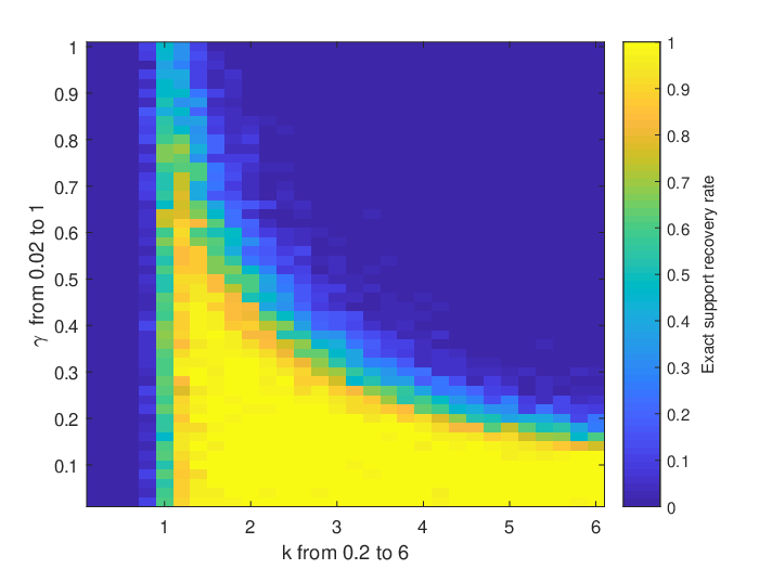
In the first simulation, we determine the effective range of λ\lambda for exact support recovery. Theoretically, (II.2) provides a lower bound for λ\lambda such that Theorem II.1 holds and (II.4) gives an upper bound to achieve exact support recovery. To verify the bounds of λ\lambda, we define γ0=σ2​μm​a​x2​K​[log⁡(M−J)+log⁡(N)]\gamma_{0}=\sqrt{\sigma^{2}\mu_{max}^{2}K\left[\log(M-J)+\log(N)\right]} and γ=γ0minj∈T⁡‖𝒙0,j‖2\gamma=\frac{\gamma_{0}}{\min_{j\in T}||\bm{x}_{0,j}||_{2}}. (II.2) implies that we could set λ=k​γ0\lambda=k\gamma_{0} for some k>0k>0. In addition, according to (II.2) and (II.4) in Theorem II.1, when all system parameters except λ\lambda are fixed, to achieve exact support recovery, λ\lambda should satisfy

C1​γ0≤λ=k​γ0<minj∈T⁡‖𝒙0,j‖2−C2C3\displaystyle C_{1}\gamma_{0}\leq\lambda=k\gamma_{0}<\frac{\min_{j\in T}||\bm{x}_{0,j}||_{2}-C_{2}}{C_{3}} (IV.1)

which is equivalent to

C1≤k<C4γ−C5\displaystyle C_{1}\leq k<\frac{C_{4}}{\gamma}-C_{5}

where C4=1C3C_{4}=\frac{1}{C_{3}} and C5=C2C3​γ0C_{5}=\frac{C_{2}}{C_{3}\gamma_{0}}. To examine this relation, we fix σ=0.1\sigma=0.1, J=K=3J=K=3, N=100N=100, and M=150M=150, and we vary kk and γ\gamma. 50 trials are run for each (k,γ)(k,\gamma) pair and we record the exact support recovery rate in Fig. 1, from which we do observe that kk should be larger than a constant which is approximately 1.21.2 under this setting and that kk has a reciprocal relation with γ\gamma.

Refer to caption
Fig. 1: The relation between kk and γ\gamma in terms of the exact support recovery rate where λ=k​γ0\lambda=k\gamma_{0} and γ=γ0minj∈T⁡‖𝒙0,j‖2\gamma=\frac{\gamma_{0}}{\min_{j\in T}||\bm{x}_{0,j}||_{2}}.

IV-B Number of Observations NN for Exact Support Recovery

Equation (II.1) in Theorem II.1 indicates that the sufficient number of observations, NN, scales nearly linearly with respect to the subspace dimension KK and the sparsity JJ. To verify that, in the second simulation, we set M=150M=150, k=3k=3, and γ=0.02\gamma=0.02 to make sure that λ\lambda is in an appropriate range for exact support recovery. We vary NN and KK (with fixed J=3J=3) and record the exact support recovery rate in Fig. 2. The result of a similar simulation but varying NN and JJ (with fixed K=3K=3) is shown in Fig. 3. 50 simulations are run for each setting. We observe that linear scaling of the number of observations NN with the subspace dimension KK and the sparsity JJ is sufficient for exact support recovery.

Refer to caption
Fig. 2: The nearly linear relation between the number of observations, NN, and the subspace dimension, KK, to achieve exact support recovery.
Refer to caption
Fig. 3: The nearly linear relation between the number of observations, NN, and the sparsity, JJ, to achieve exact support recovery.

IV-C Recovery Error Bound

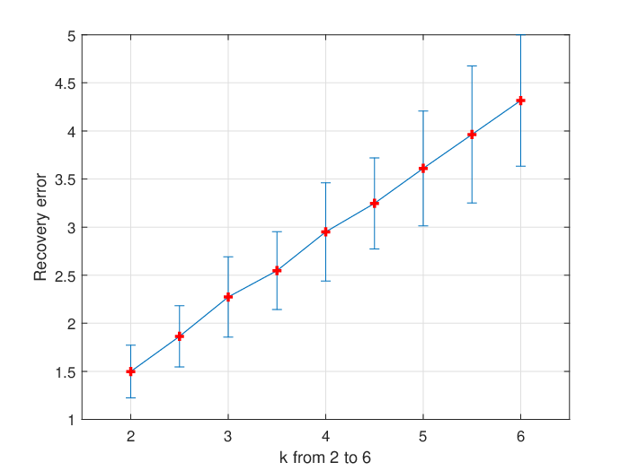
Next we turn to verify the recovery error bound in (II.3), which scales linearly with respect to λ\lambda and nearly linearly with respect to J\sqrt{J}. We set K=3K=3, N=100N=100, M=150M=150, and γ=0.02\gamma=0.02. In Fig. 4, we use λ=k​γ0\lambda=k\gamma_{0} (with fixed J=3J=3) and vary kk within the proper range for exact support recovery based on Fig. 1. 100 trials are run for each kk and we calculate the mean and standard deviation of the recovery error ‖𝐗^−𝐗0‖2,∞||\hat{\mathbf{X}}-\mathbf{X}_{0}||_{2,\infty}. Note that the recovery error is counted only when the exact support recovery is achieved. In this figure, we do observe linear scaling of the error with λ\lambda.

Similarly, we vary JJ (with fixed λ=3​γ0\lambda=3\gamma_{0}) within the proper range for exact support recovery based on Fig. 3 and record the squared recovery error ‖𝐗^−𝐗0‖2,∞2||\hat{\mathbf{X}}-\mathbf{X}_{0}||_{2,\infty}^{2} in Fig. 5. Again, the squared recovery error is counted only when the exact support recovery is achieved. In this figure, we can observe nearly linear scaling of the squared error with JJ.

Refer to caption
Fig. 4: The linear relation between the recovery error, ‖𝐗^−𝐗0‖2,∞||\hat{\mathbf{X}}-\mathbf{X}_{0}||_{2,\infty}, and the regularization parameter λ=k​γ0\lambda=k\gamma_{0}. The red plus signs and the blue horizontal sticks indicates the mean and standard deviation of the recovery error.
Refer to caption
Fig. 5: The nearly linear relation between the squared recovery error, ‖𝐗^−𝐗0‖2,∞2||\hat{\mathbf{X}}-\mathbf{X}_{0}||^{2}_{2,\infty}, and the sparsity JJ. The red plus signs and the blue horizontal sticks indicates the mean and standard deviation of the squared recovery error.

IV-D Single Molecule Imaging

In this experiment, we apply our signal model (I.1) to the single molecule imaging problem and achieve super-resolution by solving (I.5). In molecule imaging via stochastic optical reconstruction microscopy (STORM) [37], the sub-cellular structures are dyed using fluorophores, and during each observation only a small portion of the fluorophores are activated. Moreover, fluorophores at different depths will undergo different degrees of blurring.

Consequently, each observed image frame consists of a few activated fluorophores convolved with the non-stationary Gaussian point spread functions of the microscope as shown in Fig. 6 (a). Specifically, the observed low resolution frame is of size 64×6464\times 64 pixels and each pixel corresponds to a region of size 100×\times100 nm. The goal is to construct a target image with 320×320320\times 320 pixels with each pixel corresponding to a region of size 20×2020\times 20 nm.

If we vectorize the frames, each observed low resolution frame can be represented as

𝒚=S​a​m​p​l​e​[∑j=1Mcj​(𝐁′​𝒉j)⊛𝒆j+𝒏′]∈𝐑N×1\displaystyle\bm{y}=Sample\left[\sum_{j=1}^{M}c_{j}(\mathbf{B}^{\prime}\bm{h}_{j})\circledast\bm{e}_{j}+\bm{n}^{\prime}\right]\in\mathbf{R}^{N\times 1} (IV.2)

where S​a​m​p​l​e​[⋅]Sample[\cdot] indicates the sub-sampling operator, N=64×64=4096N=64\times 64=4096, and M=320×320=102400M=320\times 320=102400. Moreover, cjc_{j} is the unknown fluorophore intensity at the jj-th position, 𝐁′\mathbf{B}^{\prime} models the subspace containing the non-stationary Gaussian point spread functions (with unknown coefficient vector 𝒉j\bm{h}_{j} for the jj-th position), 𝒆j∈𝐑M\bm{e}_{j}\in\mathbf{R}^{M} is the jj-th column of the identity matrix, and 𝒏′\bm{n}^{\prime} is the unknown additive noise. All observed frames, 𝒚\bm{y}, come from the Single-Molecule Localization Microscopy grand challenge organized by ISBI [38]. The dataset contains 12000 low resolution frames, and the maximum number of activated fluorophores in each frame is 18 which implies that at most J=18J=18 coefficients cjc_{j} are non-zero for each 𝒚\bm{y}.

To apply our model, we must construct the subspace, 𝐁′\mathbf{B}^{\prime}, to capture the non-stationary point spread functions. By changing the variances (widths), we generate nine different Gaussian point spread functions; four examples are shown in Fig. 6 (b). We then apply the singular value decomposition (SVD) to a matrix of the vectorized point spread functions and record their singular values in Fig. 6 (c). From this we see that the point spread functions approximately live in a 3 dimensional subspace. Therefore, we set K=3K=3 and let 𝐁′\mathbf{B}^{\prime} contain the singular vectors corresponding to the 3 largest singular values. We display the corresponding singular vectors in Fig. 6 (d).

Refer to caption
(a)
Refer to caption
(b)
Refer to caption
(c)
Refer to caption
(d)
Fig. 6: The analysis of point spread functions. (a) A typical observed frame is of size 64×6464\times 64 pixels with each pixel corresponding to a region of size 100×100100\times 100 nm. (b) Four examples of the non-stationary point spread functions. (c) The singular values of the point spread functions. (d) The singular vectors corresponding to the three largest singular values.

To better illustrate the connection between the single molecule imaging problem and the signal model we study, (IV.2) can be equivalently represented as

𝒚=S​a​m​p​l​e​{​I​D​F​T​[∑j=1Mcj​𝐃j​𝒂j+𝒏]​}∈𝐑N×1\displaystyle\bm{y}=Sample\hbox{$\left\{\vbox to0.0pt{}\right.$}IDFT\left[\sum_{j=1}^{M}c_{j}\mathbf{D}_{j}\bm{a}_{j}+\bm{n}\right]\hbox{$\left\}\vbox to0.0pt{}\right.$}\in\mathbf{R}^{N\times 1}

where I​D​F​T​[⋅]IDFT[\cdot] denotes the inverse discrete Fourier transform operator, 𝐃j=diag(𝐁​𝒉j)\mathbf{D}_{j}=\operatorname*{diag}(\mathbf{B}\bm{h}_{j}) where 𝐁=D​F​T​[𝐁′]\mathbf{B}=DFT[\mathbf{B}^{\prime}], 𝒂j\bm{a}_{j}s are the DFTs of spikes at all possible spatial locations, and 𝒏=D​F​T​[𝒏′]\bm{n}=DFT[\bm{n}^{\prime}]. In this case, if we represent 𝒚=ℒ⁡(𝐗)\bm{y}=\mathcal{L}(\mathbf{X}) with 𝐗=[c1​𝒉1,⋯,cM​𝒉M]\mathbf{X}=[c_{1}\bm{h}_{1},\cdots,c_{M}\bm{h}_{M}], the linear operator ℒ\mathcal{L} incorporates additional inverse Fourier transform and sub-sample operators, and 𝐀\mathbf{A} is a Fourier dictionary instead of random Gaussian. The noise 𝒏\bm{n}, 𝒉j\bm{h}_{j}, and cjc_{j} for all jj are unknown, and the indices of the non-zero columns in 𝐗\mathbf{X} indicate the locations of the activated fluorophores in the high resolution image.

We pre-process each low resolution frame by subtracting the average intensity of the data set, and superimposing all the frame results in the low resolution image in Fig. 7 (a). Moreover, we solve (I.5) for each observed low resolution frame via SpaRSA [39]. By superimposing all the high resolution images that we get, we obtain the super-resolution result in Fig. 7 (b). Although the dictionary is not Gaussian in this application, the superior super-resolution result verifies the effectiveness of the proposed signal model and minimization problem.

Refer to caption
(a)
Refer to caption
(b)
Fig. 7: The single molecule imaging experiment. The image in (a) is of size 64×6464\times 64 pixels with each pixel corresponding to a region of size 100×100100\times 100 nm. (b) shows the super-resolution result, which has size 320×320320\times 320 pixels with each pixel corresponding to a region of size 20×2020\times 20 nm.

Finally, when K=1K=1, (I.5) degenerates to the classical ℓ1\ell_{1}-norm constrained lasso problem which has been comprehensively studied. However, by choosing K=1K=1, the model sacrifices its ability to capture non-stationary modulation, which is significant in this problem when the point spread functions have several comparable singular values. Although in our case, we happen to have one dominant singular value as shown in Fig. 6 (c), which implies that super-resolution can be attempted with K=1K=1, we see that a larger KK still benefits the super-resolution process. To demonstrate this, we run the single molecule imaging experiments again using K=3K=3 and K=1K=1. Three super-resolution examples are shown in Fig. 8, from which we can find that although K=3K=3 and K=1K=1 achieve similar performance, some activated fluorophores can be more accurately represented using the 3-dimensional subspace (K=3K=3), and that leads to a more clear and accurate super-resolution result.

Refer to caption
(a)
Refer to caption
(b)
Refer to caption
(c)
Refer to caption
(d)
Refer to caption
(e)
Refer to caption
(f)
Refer to caption
(g)
Refer to caption
(h)
Refer to caption
(i)
Fig. 8: Comparison between the super-resolution results for K=3K=3 and K=1K=1. (a), (d), and (g) are three low-resolution input frames. (b), (e), and (h) show the super-resolution results for K=3K=3. (c), (f), and (i) show the super-resolution results for K=1K=1. The area of interest is highlighted using the red rectangle. The input frames are of size 64×6464\times 64 pixels and the outputs are 320×320320\times 320 pixels.

V Conclusion

In this paper, we consider the problem of recovering a sparse signal with unbounded noise and non-stationary blind modulation. Using the lifting technique and with a subspace assumption on the modulating signals, we recast this problem as the recovery of a column-wise sparse matrix from structured linear observations. We apply ℓ2,1\ell_{2,1}-norm regularized quadratic minimization, also known as the group lasso, to solve this problem and derive sufficient conditions on the sample complexity and regularization parameter for exact support recovery. We also bound the recovery error in terms of the ℓ2,∞\ell_{2,\infty}-norm. Numerical simulations are consistent with our predictions and support the theoretical results. Moreover, we apply our model to single molecule imaging and achieve promising super-resolution results. One useful generalization of the results in this paper would be to consider the random Fourier dictionary. Allowing 𝐃j\mathbf{D}_{j} to be non-diagonal but live in a low-dimensional matrix subspace is another important generalization, which could open up other potential applications.

Acknowledgment

This work was supported by NSF grant CCF−1704204-1704204.

References

  • [1] Y. Xie, M. B. Wakin, and G. Tang, “Support recovery for sparse recovery and non-stationary blind demodulation,” in 2019 53rd Asilomar Conference on Signals, Systems and Computers, IEEE, 2019.
  • [2] H. Mansour, D. Liu, P. T. Boufounos, and U. S. Kamilov, “Radar autofocus using sparse blind deconvolution,” in 2018 IEEE International Conference on Acoustics, Speech and Signal Processing (ICASSP), pp. 1623–1627, IEEE, 2018.
  • [3] M. Lustig, D. Donoho, and J. M. Pauly, “Sparse mri: The application of compressed sensing for rapid mr imaging,” Magnetic Resonance in Medicine: An Official Journal of the International Society for Magnetic Resonance in Medicine, vol. 58, no. 6, pp. 1182–1195, 2007.
  • [4] H. Mansour and Ö. Yilmaz, “Adaptive compressed sensing for video acquisition,” in 2012 IEEE International Conference on Acoustics, Speech and Signal Processing (ICASSP), pp. 3465–3468, IEEE, 2012.
  • [5] E. J. Candès and M. B. Wakin, “An introduction to compressive sampling,” IEEE Signal Processing Magazine, vol. 25, no. 2, pp. 21–30, 2008.
  • [6] E. J. Candes and Y. Plan, “A probabilistic and ripless theory of compressed sensing,” IEEE Transactions on Information Theory, vol. 57, no. 11, pp. 7235–7254, 2011.
  • [7] Y. Xie, S. Li, G. Tang, and M. B. Wakin, “Radar signal demixing via convex optimization,” in 2017 22nd International Conference on Digital Signal Processing (DSP), pp. 1–5, IEEE, 2017.
  • [8] Y. Xie, M. B. Wakin, and G. Tang, “Simultaneous sparse recovery and blind demodulation,” IEEE Transactions on Signal Processing, vol. 67, no. 19, pp. 5184–5199, 2019.
  • [9] S. Ling and T. Strohmer, “Self-calibration and biconvex compressive sensing,” Inverse Problems, vol. 31, no. 11, p. 115002, 2015.
  • [10] A. Ahmed, B. Recht, and J. Romberg, “Blind deconvolution using convex programming,” IEEE Transactions on Information Theory, vol. 60, no. 3, pp. 1711–1732, 2014.
  • [11] H. Zou, “The adaptive lasso and its oracle properties,” Journal of the American statistical association, vol. 101, no. 476, pp. 1418–1429, 2006.
  • [12] M. Yuan and Y. Lin, “Model selection and estimation in regression with grouped variables,” Journal of the Royal Statistical Society: Series B (Statistical Methodology), vol. 68, no. 1, pp. 49–67, 2006.
  • [13] B. Friedlander and T. Strohmer, “Bilinear compressed sensing for array self-calibration,” in 2014 48th Asilomar Conference on Signals, Systems and Computers, pp. 363–367, IEEE, 2014.
  • [14] D. Yang, G. Tang, and M. B. Wakin, “Super-resolution of complex exponentials from modulations with unknown waveforms,” IEEE Transactions on Information Theory, vol. 62, no. 10, pp. 5809–5830, 2016.
  • [15] G. Tang, B. N. Bhaskar, and B. Recht, “Sparse recovery over continuous dictionaries-just discretize,” in 2013 Asilomar Conference on Signals, Systems and Computers, pp. 1043–1047, IEEE, 2013.
  • [16] S. Ling and T. Strohmer, “Blind deconvolution meets blind demixing: Algorithms and performance bounds,” IEEE Transactions on Information Theory, vol. 63, no. 7, pp. 4497–4520, 2017.
  • [17] Y. Chi, “Guaranteed blind sparse spikes deconvolution via lifting and convex optimization,” J. Sel. Topics Signal Processing, vol. 10, no. 4, pp. 782–794, 2016.
  • [18] S. Ling and T. Strohmer, “Self-calibration and bilinear inverse problems via linear least squares,” SIAM Journal on Imaging Sciences, vol. 11, no. 1, pp. 252–292, 2018.
  • [19] A. Aghasi, A. Ahmed, P. Hand, and B. Joshi, “A convex program for bilinear inversion of sparse vectors,” in Advances in Neural Information Processing Systems, pp. 8548–8558, 2018.
  • [20] M. S. Asif, W. Mantzel, and J. Romberg, “Random channel coding and blind deconvolution,” in 2009 47th Annual Allerton Conference on Communication, Control, and Computing (Allerton), pp. 1021–1025, IEEE, 2009.
  • [21] Y. Xie, M. B. Wakin, and G. Tang, “Sparse recovery and non-stationary blind demodulation,” in ICASSP 2019-2019 IEEE International Conference on Acoustics, Speech and Signal Processing (ICASSP), pp. 5566–5570, IEEE, 2019.
  • [22] Y. Nardi, A. Rinaldo, et al., “On the asymptotic properties of the group lasso estimator for linear models,” Electronic Journal of Statistics, vol. 2, pp. 605–633, 2008.
  • [23] X. Lv, G. Bi, and C. Wan, “The group lasso for stable recovery of block-sparse signal representations,” IEEE Transactions on Signal Processing, vol. 59, no. 4, pp. 1371–1382, 2011.
  • [24] J. Huang, T. Zhang, et al., “The benefit of group sparsity,” The Annals of Statistics, vol. 38, no. 4, pp. 1978–2004, 2010.
  • [25] V. Sivakumar, A. Banerjee, and P. K. Ravikumar, “Beyond sub-gaussian measurements: High-dimensional structured estimation with sub-exponential designs,” in Advances in neural information processing systems, pp. 2206–2214, 2015.
  • [26] S. Vaiter, M. Golbabaee, J. Fadili, and G. Peyré, “Model selection with low complexity priors,” Information and Inference: A Journal of the IMA, vol. 4, no. 3, pp. 230–287, 2015.
  • [27] S. Vaiter, G. Peyré, and J. Fadili, “Model consistency of partly smooth regularizers,” IEEE Transactions on Information Theory, vol. 64, no. 3, pp. 1725–1737, 2017.
  • [28] C.-Y. Hung and M. Kaveh, “Low rank matrix recovery for joint array self-calibration and sparse model doa estimation,” in 2017 IEEE 7th International Workshop on Computational Advances in Multi-Sensor Adaptive Processing (CAMSAP), pp. 1–5, IEEE, 2017.
  • [29] Y. C. Eldar, W. Liao, and S. Tang, “Sensor calibration for off-the-grid spectral estimation,” Applied and Computational Harmonic Analysis, 2018.
  • [30] A. Flinth, “Sparse blind deconvolution and demixing through ℓ1,2\ell_{1,2}-minimization,” Advances in Computational Mathematics, vol. 44, no. 1, pp. 1–21, 2018.
  • [31] T. Hastie, R. Tibshirani, and M. Wainwright, Statistical learning with sparsity: the lasso and generalizations. Chapman and Hall/CRC, 2015.
  • [32] M. J. Wainwright, “Sharp thresholds for high-dimensional and noisy sparsity recovery using ℓ1\ell_{1}-constrained quadratic programming (lasso),” IEEE Transactions on Information Theory, vol. 55, no. 5, pp. 2183–2202, 2009.
  • [33] S. Foucart and H. Rauhut, A mathematical introduction to compressive sensing. Birkhäuser Basel, 2013.
  • [34] D. Hsu, S. Kakade, T. Zhang, et al., “A tail inequality for quadratic forms of subgaussian random vectors,” Electronic Communications in Probability, vol. 17, 2012.
  • [35] B. Laurent and P. Massart, “Adaptive estimation of a quadratic functional by model selection,” Annals of Statistics, pp. 1302–1338, 2000.
  • [36] M. Grant, S. Boyd, and Y. Ye, “Cvx: Matlab software for disciplined convex programming,” 2008.
  • [37] M. J. Rust, M. Bates, and X. Zhuang, “Sub-diffraction-limit imaging by stochastic optical reconstruction microscopy (storm),” Nature methods, vol. 3, no. 10, p. 793, 2006.
  • [38] EPFL-Biomedical-Imaging-Group, “Single-molecule localization microscopy,” http://bigwww.epfl.ch/smlm/, 2013.
  • [39] S. J. Wright, R. D. Nowak, and M. A. Figueiredo, “Sparse reconstruction by separable approximation,” IEEE Transactions on Signal Processing, vol. 57, no. 7, pp. 2479–2493, 2009.