se counter=example]example[2][]title=Example \thetcbcounter: #2,#1
Active Subspace of Neural Networks: Structural Analysis and Universal Attacks Thanks: Submitted to the editors on October 2019.
Chunfeng Cui
Email: chunfengcui@ucsb.eduEmail: kzhang07@ucsb.eduEmail: zhengzhang@ece.ucsb.eduThanks: University of California Santa Barbara, Santa Barbara, CA, USA
(, ,
).
Kaiqi Zhang22footnotemark: 2Talgat Daulbaev
Email: talgat.daulbaev@skoltech.ruEmail: y.gusak@skoltech.ruThanks: Skolkovo Institute of Science and Technology, Moscow, Russia
(,
).
Julia Gusak33footnotemark: 3 Ivan Oseledets
Email: ivan.oseledets@gamil.comThanks: Skolkovo Institute of Science and Technology and Institute of Numerical Mathematics of Russian Academy of Sciences, Moscow, Russia (.)
Zheng Zhang22footnotemark: 2
Abstract
Active subspace is a model reduction method widely used in the uncertainty quantification community. In this paper, we propose analyzing the internal structure and vulnerability of deep neural networks using active subspace.
Firstly, we employ the active subspace to measure the number of “active neurons” at each intermediate layer, which indicates that the number of neurons can be reduced from several thousands to several dozens. This motivates us to change the network structure and to develop a new and more compact network, referred to as ASNet, that has significantly fewer model parameters. Secondly, we propose analyzing the vulnerability of a neural network using active subspace by finding an additive universal adversarial attack vector that can misclassify a dataset with a high probability.
Our experiments on CIFAR-10 show that ASNet can achieve 23.98 parameter and 7.30 flops reduction. The universal active subspace attack vector can achieve around 20% higher attack ratio compared with the existing approaches in our numerical experiments.
The PyTorch codes for this paper are available online 111
Codes are available at: https://github.com/chunfengc/ASNet.
keywords
Active Subspace, Deep Neural Network, Network Reduction, Universal Adversarial Perturbation
Funding.
Chunfeng Cui, Kaiqi Zhang, and Zheng Zhang are supported by the UCSB start-up grant.
Talgat Daulbaev, Julia Gusak, and Ivan Oseledets are supported by the Ministry of Education and Science of the Russian Federation (grant 14.756.31.0001).
††runningheads: Active Subspace of Neural Networks: Structural Analysis and Universal Attacks / C. Cui, K. Zhang, T. Daulbaev, J. Gusak, I. Oseledets, and Z. Zhang
AMS
90C26, 15A18, 62G35
1 Introduction
Deep neural networks have achieved impressive performance in many applications, such as computer vision [35], nature language processing [58], and speech recognition [23]. Most neural networks use deep structure (i.e., many layers) and a huge number of neurons to achieve a high accuracy and expressive power [44, 19].
However, it is still unclear how many layers and neurons are necessary. Employing an unnecessarily complicated deep neural network can cause huge extra costs in run-time and hardware resources. Driven by resource-constrained applications such as robotics and internet of things, there is an increasing interest in building smaller neural networks by removing network redundancy. Representative methods include network pruning and sharing [17, 25, 27, 39, 38], low-rank matrix and tensor factorization [49, 26, 18, 36, 43], parameter quantization [12, 15], knowledge distillation [28, 46], and so forth.
However, most existing methods delete model parameters directly without changing the network architecture [27, 25, 7, 38].
Another important issue of deep neural networks is the lack of robustness.
A deep neural network is desired to maintain good performance for noisy or corrupted data to be deployed in safety-critical applications such as autonomous driving and medical image analysis.
However, recent studies have revealed that many state-of-the-art deep neural networks are vulnerable to small perturbations [54].
A substantial number of methods have been proposed to generate adversarial examples. Representative works can be classified into four classes [52], including
optimization methods [8, 41, 40, 54],
sensitive features [22, 45], geometric transformations [16, 32],
and generative models [4].
However, these methods share a fundamental limitation: each perturbation is designed for a given data point, and one has to implement the algorithm again to generate the perturbation for a new data sample.
Recently, several methods have also been proposed to compute a universal adversarial attack to fool a dataset simultaneously (rather than one data sample) in various applications, such as computer vision [40], speech recognition [42], audio [1], and text classifier [5].
However, all the above methods only solve a series of data-dependent sub-problems.
In [33], Khrulkov et al. proposed to construct universal perturbation by computing the so-called -singular vectors of the Jacobian matrices of hidden layers of a network.
This paper investigates the above two issues with the active subspace method [48, 9, 10] that was originally developed for uncertainty quantification. The key idea of the active subspace is to identify the low-dimensional subspace constructed by some important directions that can contribute significantly to the variance of the multi-variable function.
These directions are corresponding to the principal components of the uncentered covariance matrix of gradients. Afterwards, a response surface can be constructed in this low-dimensional subspace to reduce the number of parameters for partial differential equations [10] and uncertainty quantification [11]. However, the power of active subspace in analyzing and attacking deep neural networks has not been explored.
1.1 Paper Contributions
The contribution of this manuscript is twofold.
•
Firstly, we apply the active subspace to some intermediate layers of a deep neural network, and try to answer the following question: how many neurons and layers are important in a deep neural network?
Based on the active subspace, we propose the definition of “active neurons”.
Fig. 1 (a) shows that even though there are tens of thousands of neurons, only dozens of them are important from the active subspace point of view.
Fig. 1 (b) further shows that most of the neural network parameters are distributed in the last few layers. This motivates us to cut off the tail layers and replace them with a smaller and simpler new framework called ASNet. ASNet contains three parts: the first few layers of a deep neural network, an active-subspace layer that maps the intermediate neurons to a low-dimensional subspace, and a polynomial chaos expansion layer that projects the reduced variables to the outputs.
Our numerical experiments show that the proposed ASNet has much fewer model parameters than the original one.
ASNet can also be combined with existing structured re-training methods (e.g., pruning and quantization) to get better accuracy while using fewer model parameters.
•
Secondly, we use active subspace to develop a new universal attack method to fool deep neural networks on a whole data set.
We formulate this problem as a ball-constrained loss maximization problem and propose a heuristic projected gradient descent algorithm to solve it. At each iteration, the ascent direction is the dominant active subspace, and the stepsize is decided by the backtracking algorithm.
Fig. 1 (c) shows that the attack ratio of the active subspace direction is much higher than that of the random vector.
Figure 1: Structural analysis of deep neural networks by the active subspace (AS). All experiments are conducted on CIFAR-10 by VGG-19. (a) The number of neurons can be significantly reduced by the active subspace.
Here, the number of active neurons is defined by Definition 3.1 with a threshold ; (b) Most of the parameters are distributed in the last few layers; (c) The active subspace direction can perturb the network significantly.
The rest of this manuscript is
organized as follows. In Section 2, we review the key idea of active subspace. Based on the active-subspace method, Section 3 shows how to find the number of active neurons in a deep neural network and further proposes a new and compact network, referred to as ASNet. Section 4 develops a new universal adversarial attack method based on active subspace. The numerical experiments for both ASNet and universal adversarial attacks are presented in Section 5. Finally, we conclude this paper in Section 6.
2 Active Subspace
Active-subspace is an efficient tool for functional analysis and dimension reduction.
Its key idea is to construct a low-dimensional subspace for the input variables in which the function value changes dramatically.
Given a continuous function ) with described by the probability density function , one can construct an uncentered covariance matrix for the gradient: .
Suppose the matrix admits the following eigenvalue decomposition,
(1)
where includes all orthogonal eigenvectors and
(2)
are the eigenvalues.
All the eigenvalues are nonnegative because is positive semidefinite. One can split the matrix into two parts,
(3)
The subspace spanned by matrix is called an active subspace [48], because is sensitive to perturbation vectors inside this subspace .
Remark 1 (Relationships with the Principal Component Analysis).
Given a set of data with each column representing a data sample and each row is zero-mean, the first principal component inherits the maximal variance from , namely,
(4)
The variance is maximized when is the eigenvector associated with the largest eigenvalue of .
The first principal components are the eigenvectors associated with the largest eigenvalues of .
The main difference with the active subspace is that the principal component analysis uses the covariance matrix of input data sets , but the active-subspace method uses the covariance matrix of gradient .
Hence, a perturbation along the direction from (4) only guarantee the variability in the data, and does not necessarily cause a significantly change on the value of .
The following lemma quantitatively describes that varies more on average along the directions defined by the columns of than the directions defined by the columns of .
Lemma 2.
[10]
Suppose is a continuous function and is obtained from (1). For the matrices and generated by (3), and the reduced vector
When , Lemma 2 implies is zero everywhere, i.e., is -invariant.
In this case, we may reduce to a low-dimensional vector and construct a new response surface to represent .
Otherwise, if is small, we may still construct a response surface to approximate with a bounded error, as shown in the following lemma.
2.1 Response Surface
For a fixed , the best guess for is the conditional expectation of given , i.e.,
(7)
Based on the Poincaré inequality, the following approximation error bound is obtained [10].
Lemma 3.
Assume that is absolutely continuous and square integrable with respect to the probability density function , then the approximation function in (7) satisfies:
In other words, the active-subspace approximation error will be small if are negligible.
3 Active Subspace for Structural Analysis and Compression of Deep Neural Networks
This section applies the active subspace to analyze the internal layers of a deep neural network to reveal the number of important neurons at each layer. Afterward, a new network called ASNet is built to reduce the storage and computational complexity.
3.1 Deep Neural Networks
A deep neural network can be described as
(9)
where is an input, is the total number of layers, and is a function representing the -th layer (e.g., combinations of convolution or fully connected, batch normalization, ReLU, or pooling layers).
For any , we rewrite the above feed-forward model as a superposition of functions, i.e.,
(10)
where the pre-model denotes all operations before the -th layer and the post-model denotes all succeeding operations.
The intermediate neuron usually lies in a high dimension. We aim to study whether such a high dimensionality is necessary. If not, how can we reduce it?
3.2 The Number of Active Neurons
Denote as the loss function, and
(11)
The covariance matrix admits the eigenvalue decomposition with .
We try to extract the active subspace of and reduce the intermediate vector to a low dimension.
Here the intermediate neuron , the covariance matrix , eigenvalues , and eigenvectors are also related to the layer index , but we ignore the index for simplicity.
Definition 3.1.
Suppose is computed by (2). For any layer index , we define the number of active neurons as follows:
(12)
where is a user-defined threshold.
Based on Definition 3.1, the post-model can be approximated by an -dimensional function with a high accuracy, i.e.,
(13)
Here plays the role of active neurons, , and .
Lemma 4.
Suppose the input is bounded. Consider a deep neural network with the following operations: convolution, fully connected, ReLU, batch normalization, max-pooling, and equipped with the cross entropy loss function. Then for any , , and , the -dimensional function defined in (13) satisfies
(14)
Proof.
Denote , where is the cross entropy loss function, is the true label, and is the total number of classes.
We first show is absolutely continuous and square integrable, and then apply Lemma 3 to derive (14).
Firstly, all components of are Lipschitz continuous because (1) the convolution, fully connected, and batch normalization operations are all linear; (2) the max pooling and ReLU functions are non-expansive. Here, a mapping is non-expansive if ; (3) the cross entropy loss function is smooth with an upper bounded gradient, i.e., . The composition of two Lipschitz continuous functions is also be Lipschitz continuous: suppose the Lipschitz constants for and are and , respectively, it holds that for any vectors and .
By recursively applying the above rule, is Lipschitz continuous:
The intermediate neuron is in a bounded domain because the input is bounded and all functions are either continuous or non-expansive.
Based on the fact that any Lipschitz-continuous function is also absolutely continuous on a compact domain [47], we conclude that is absolutely continuous.
Secondly, because is bounded and is continuous, both and its square integral will be bounded, i.e.,
.
In the last equality, we used that is upper bounded because is Lipschitz continuous with a bounded gradient.
Consequently, we have
The proof is completed.
The above lemma shows that the active subspace method can reduce the number of neurons of the -th layer from to .
The loss for the low-dimensional function is bounded by two terms: the loss of the original network, and the threshold related to .
This loss function is the cross entropy loss, not the classification error.
However, it is believed that a small loss will result in a small classification error.
Further, the result in Lemma 4 is valid for thr fixed parameters in the pre-model.
In practice, we can fine-tune the pre-model to achieve better accuracy.
Further, a small active neurons is critical to get a high compress ratio.
From Definition 3.1, depends on the eigenvalue distribution of the covariance matrix .
For a proper network structure and a good choice of the layer index , if the eigenvalues of are dominated by the first few eigenvalues,
then will be small. For instance, in Fig. 5(a), the eigenvalues for layers of VGG-19 are nearly exponential decreasing to zero.
3.3 Active Subspace Network (ASNet)
Algorithm 1 The training procedure of the active subspace network (ASNet)
Input: A pretrained deep neural network, the layer index , and the number of active neurons .
Step 1
Initialize the active subspace layer.
The active subspace layer is a linear projection where the projection matrix is computed by Algorithm 2.
If is not given, we use defined in (12) by default.
Step 2
Initialize the polynomial chaos expansion layer. The polynomial chaos expansion layer is a nonlinear mapping from the reduced active subspace to the outputs, as shown in (18).
The weights is computed by (20).
Step 3
Construct the ASNet. Combine the pre-model (the first layers of the deep neural network) with the active subspace and polynomial chaos expansion layers as a new network, referred to as ASNet.
Step 4
Fine-tuning. Retrain all the parameters in pre-model, active subspace layer and polynomial chaos expansion layer in ASNet for several epochs by stochastic gradient descent.
Output: A new network ASNet
This subsection proposes a new network called ASNet that can reduce both the storage and computational cost.
Given a deep neural network, we first choose a proper layer and project the high-dimensional intermediate neurons to a low-dimensional vector in the active subspace. Afterward, the post-model is deleted completely and replaced with a nonlinear model that maps the low-dimensional active feature vector to the output directly. This new network, called ASNet, has three parts:
(1)
Pre-model: the pre-model includes the first layers of a deep neural network.
(2)
Active subspace layer: a linear projection from the intermediate neurons to the low-dimensional active subspace.
(3)
Polynomial chaos expansion layer: the polynomial chaos expansion [20, 56] maps the active-subspace variables to the output.
The initialization for the active subspace layer and polynomial chaos expansion layer are presented in Sections 3.4 and 3.5, respectively.
We can also retrain all the parameters to increase the accuracy.
The whole procedure is illustrated in Fig. 2 (b) and Algorithm 1.
(a)A deep neural network
(b)The proposed ASNet
Figure 2: (a) The original deep neural network; (b) The proposed ASNet with three parts: a pre-model, an active subspace (AS) layer, and a polynomial chaos expansion (PCE) layer.
3.4 The Active Subspace Layer
This subsection presents an efficient method to project the high dimensional neurons to the active subspace.
Given a dataset , the empirical covariance matrix is computed by .
When ReLU is applied as an activation, is not differentiable.
In this case, denotes the sub-gradient with a little abuse of notation.
Instead of calculating the eigenvalue decomposition of , we compute the singular value decomposition of to save the computation cost:
(15)
The eigenvectors of are approximated by the left singular vectors and the eigenvalues of are approximated by the singular values of , i.e., .
We use the memory-saving frequent direction method [21] to compute the dominant singular value components, i.e., . Here is smaller than the total number of samples.
The frequent direction approach only stores an matrix .
At the beginning, each column of is initialized by a gradient vector.
Then the randomized singular value decomposition [24] is used to generate .
Afterwards, is updated in the following way,
(16)
Now the last column of is zero and we replace it with the gradient vector of a new sample.
By repeating this process, will approximate with a high accuracy and will approximate the left singular vectors of .
The algorithm framework is presented in Algorithm 2.
Algorithm 2 The frequent direction algorithm for computing the active subspace
Input: A dataset with input samples , a pre-model , a subroutine for computing , and the dimension of truncated singular value decomposition .
1:
Select samples , compute , and construct an initial matrix .
2:for t=1, 2, do
3:
Compute the singular value decomposition , where .
4:
If the maximal number of samples is reached, stop.
6:
Get a new sample , compute , and replace the last column of (now all zeros) by the gradient vector .
7:endforOutput: The projection matrix and the singular values .
After obtaining , we can approximate the number of active neurons as
(17)
Under the condition that for and for ,
(17) can approximate in (12) with a high accuracy.
Further, the projection matrix is chosen as the first columns of .
The storage cost is reduced from to and the computational cost is reduced from to .
3.5 Polynomial Chaos Expansion Layer
We continue to construct a new surrogate model to approximate the post-model of a deep neural network.
This problem can be regarded as an uncertainty quantification problem if we set as a random vector.
We choose the nonlinear polynomial because it has higher expressive power than linear functions.
By the polynomial chaos expansion [55], the network output is approximated by a linear combination of the orthogonal polynomial basis functions:
(18)
Here
is a multivariate polynomial basis function chosen based on the probability density function of .
When the parameters are independent, both the joint density function and the multi-variable basis function can be decomposed into products of one-dimensional functions, i.e., ,
The marginal basis function is uniquely determined by the marginal density function . The scatter plot in Fig. 3 shows that the marginal probability density of e is close to a Gaussian distribution.
Suppose follows a Gaussian distribution, then will be a Hermite polynomial [37], i.e.,
(19)
In general, the elements in can be non-Gaussian correlated. In this case, the basis functions can be built via the Gram-Schmidt approach described in [13].
Figure 3: Distribution of the first two active subspace variables at the 6-th layer of VGG-19 for CIFAR-10.
The coefficient can be computed by a linear least-square optimization.
Denote as the random samples and as the network output for . The coefficient vector can be computed by
(20)
Based on the Nyquist-Shannon sampling theorem, the number of samples to train needs to satisfy .
However, this number can be reduced to a smaller set of “important” samples by the D-optimal design [59] or the sparse regularization approach [14].
The polynomial chaos expansion builds a surrogate model to approximate the deep neural network output .
This idea is similar to the knowledge distillation [28], where a pre-trained teacher network teaches a smaller student network to learn the output feature.
However, our polynomial-chaos layer uses one nonlinear projection whereas the knowledge distillation uses a series of layers. Therefore, the polynomial chaos expansion is more efficient in terms of computational and storage cost.
The polynomial chaos expansion layer is different from the polynomial activation because the dimension of may be different from that of output .
The problem (20) is convex and any first order method can get a global optimal solution.
Denote the optimal coefficients as and the finial objective value as , i.e.,
(21)
If , the polynomial chaos expansion is a good approximation to the original deep neural network on the training dataset.
However, the approximation loss of the testing dataset may be large because of the overfitting phenomena.
The objective function in (20) is an empirical approximation to the expected error
(22)
According to the Hoeffding’s inequality [29], the expected error (22) is close to the empirical error (20) with a high probability.
Consequently, the loss for ASNet with polynomial chaos expansion layer is bounded as follows.
Lemma 5.
Suppose that the optimal solution for solving problem (20) is , the optimal polynomial chaos expansion is , and the optimal residue is .
Assume that there exist consts such that for all , .
Then the loss of ASNet will be upper bounded
(23)
where is a user-defined threshold, and .
Proof.
Since the cross entropy loss function is -Lipschitz continuous, we have
(24)
Denote for .
are independent under the assumption that the data samples are independent.
By the Hoeffding’s inequality, for any constant , it holds that
(25)
with .
Equivalently,
(26)
Consequently, there is
The last inequality follows from , equations (24) and (26).
This completes the proof.
Lemma 5 shows with a high probability , the expected error of ASNet without fine-tuning is bounded by the pre-trained error of the original network, the accuracy loss in solving the polynomial chaos subproblem (21), and the number of classes .
The probability is controlled by the threshold as well as the number of training samples .
In practice, we always re-train ASNet for several epochs and the accuracy of ASNet is beyond the scope of Lemma 5.
3.6 Structured Re-training of ASNet
The pre-model can be further compressed by various techniques such as network pruning and sharing [25], low-rank factorization [43, 36, 18], or data quantization [15, 12]. Denote as the weights in ASNet and as the training dataset.
Here, denotes all the parameters in the pre-model, active subspace layer, and the polynomial chaos expansion layer.
We re-train the network by solving the following regularized optimization problem:
(27)
Here is a training sample, is the total number of training samples, is the cross-entropy loss function, is a regularization function, and is a regularization parameter.
Different regularization functions can result in different model structures. For instance, an regularizer [2, 50, 57] will return a sparse weight, an -norm regularizer will result in a column-wise sparse weights, a nuclear norm regularizer will result in low-rank weights.
At each iteration, we solve (27) by a stochastic proximal gradient decent algorithm [53]
(28)
Here is the stochastic gradient, is a batch at the -th step, and is the stepsize.
In this work, we chose the regularization to get sparse weight matrices.
In this case, problem (28) has a closed-form solution:
(29)
where is a soft-thresholding operator.
4 Active-Subspace for Universal Adversarial Attacks
This section investigates how to generate a universal adversarial attack by the active-subspace method. Given a function , the maximal perturbation direction is defined by
(30)
Here, is a user-defined perturbation upper bound. By the first order Taylor expansion, we have , and problem (30) can be reduced to
(31)
The vector is exactly the dominant eigenvector of the covariance matrix of . The solution for (30) can be approximated by or . Here, both and are solutions of (31) but their effect on (30) are different.
Figure 4: Perturbations along the directions of an active-subspace direction and of principal component, respectively. (a) The function . (b) The perturbed function along the active-subspace direction. (c) The perturbed function along the principal component analysis direction.
Example 4.1.
Consider a two-dimensional function with and , and follows a uniform distribution in a two-dimensional square domain , as shown in Fig. 4 (a).
It follows from direct computations that and the covariance matrix . The dominant eigenvector of or the active-subspace direction is .
We apply to perturb and plot in Fig. 4 (b), which shows a significant difference even for a small permutation .
Furthermore, we plot the perturbed function along the
first principal component direction in Fig. 4 (c).
Here, is the eigenvector of the covariance matrix .
However, does not result in any perturbation because .
This example indicates the difference between the active-subspace and principal component analysis: the active-subspace direction can capture the sensitivity information of whereas the principal component is independent of .
4.1 Universal Perturbation of Deep Neural Networks
Given a dataset and a classification function that maps an input sample to an output label. The universal perturbation seeks for a vector whose norm is upper bounded by , such that the class label can be perturbed with a high probability, i.e.,
(32)
where equals one if the condition is satisfied and zero otherwise.
Solving problem (32) directly is challenging because both and are discontinuous.
By replacing with the loss function and the indicator function with a quadratic function, we reformulate problem (32) as
(33)
The ball-constrained optimization problem (33) can be solved by various numerical techniques such as the spectral gradient descent method [6] and the limited-memory projected quasi-Newton [51]. However, these methods can only guarantee convergence to a local stationary point. Instead, we are interested in computing a direction that can achieve a better objective value by a heuristic algorithm.
4.2 Recursive Projection Method
Using the first order Taylor expansion , we reformulate problem (33) as a ball constrained quadratic problem
(34)
Problem (34) is easy to solve because its closed-form solution is exactly the dominant eigenvector of the covariance matrix or the first active-subspace direction.
However, the dominant eigenvector in (34) may not be efficient because is nonlinear.
Therefore, we compute recursively by
(35)
where ,
is the stepsize, and is approximated by
(36)
Namely, is the dominant eigenvector of .
Because maximizes the changes in , we expect that the attack ratio keeps increasing, i.e., , where
(37)
The backtracking line search approach [3] is employed to choose such that the attack ratio of is higher than the attack ratio of both and , i.e.,
(38)
where , , is the initial stepsize, is the decrease ratio, and .
If such a stepsize exists, we update by (35) and repeat the process. Otherwise, we record the number of failures and stop the algorithm when the number of failure is greater than a threshold.
The overall flow is summarized in Algorithm 3.
In practice, instead of using the whole dataset to train this attack vector, we use a subset .
The impact for different number of samples is discussed in section 5.2.2.
Algorithm 3 Recursive Active Subspace Universal Attack
Input: A pre-trained deep neural network denoted as , a classification oracle , a training dataset , an upper bound for the attack vector , an initial stepsize , a decrease ratio , and the parameter in the stopping criterion .
1:
Initialize the attack vector as .
2:fordo
3:
Select the training dataset as , then compute the dominate active subspace direction by Algorithm 2.
4:fordo
5:
Let and . Compute the attack ratios and by (37).
6:
If either or is greater than , stop the process. Return , where if and otherwise.
7:endforIf no stepsize is returned, let and record this step as a failure.
Compute the next iteration by the projection (35).
8:
If the number of failure is greater the threshold , stop.
9:endforOutput: The universal active adversarial attack vector .
5 Numerical Experiments
In this section, we show the power of active-subspace in revealing the number of active neurons, compressing neural networks, and computing the universal adversarial perturbation.
All codes are implemented in PyTorch and are available online222https://github.com/chunfengc/ASNet.
5.1 Structural Analysis and Compression
We test the ASNet constructed by Algorithm 1, and set the polynomial order as , the number of active neurons as , and the threshold in Equation (12) as on default.
Inspired by the knowledge distillation [28], we retrain all the parameters in the ASNet by minimizing the following loss function
Here, the cross entropy , the softmax function , and the parameter on default.
We retrain ASNet for 50 epochs by ADAM [34].
The stepsizes for the pre-model are set as and for VGG-19 and ResNet,
and the stepsize for the active subspace layer and the polynomial chaos expansion layer is set as , respectively,
We also seek for sparser weights in ASNet by the proximal stochastic gradient descent method in Section 3.6.
On default, we set the stepsize as for the pre-model and for the active subspace layer and the polynomial chaos expansion layer. The maximal epoch is set as 100.
The obtained sparse model is denoted as ASNet-s.
In all figures and tables, the numbers in the bracket of ASNet() or ASNet-s() indicate the index of a cut-off layer.
We report the performance for different cut-off layers in terms of accuracy, storage, and computational complexities.
5.1.1 Choices of Parameters
We first show the influence of number of reduced neurons , tolerance , and cutting-off layer index of VGG-19 on CIFAR-10 in Table 1. The VGG-19 can achieve 93.28% testing accuracy with 76.45 Mb stroage consumption.
Here, .
For different choices of ,
we display the corresponding tolerance , the storage speedup compared with the original teacher network, and the testing accuracy reduction for ASNet before and after fine-tuning compared with the original teacher network.
Table 1 shows that when the cutting-off layer is fixed, a larger usually results in a smaller tolerance and a smaller accuracy reduction but also a smaller storage speedup.
This is corresponding to Lemma 4 that the error of ASNet before fine-tuning is upper bounded by .
Comparing with , we find that can achieve almost the same accuracy with with a higher storage speedup.
can even achieve better accuracy than in layer 7 probably because of overfitting. This guides us to chose in the following numerical experiments.
For different layers, we see a later cutting-off layer index can produce a lower accuracy reduction but a smaller storage speedup.
In other words, the choice of layer index is a trade-off between accuracy reduction with storage speedup.
Table 1: Comparison of number of neurons of VGG-19 on CIFAR-10. For the stroage speedup, the higher is bettter. For the accuracy reduction before or after finetuning, the lower is better.
Storage
Accu. Reduce
Storage
Accu. Reduce
Storage
Accu. Reduce
Before
After
Before
After
Before
After
ASNet(5)
0.34
20.7
7.06
2.82
0.18
14.4
4.40
1.82
0.11
11.0
3.64
1.66
ASNet(6)
0.24
12.8
2.14
0.59
0.11
10.1
1.62
0.27
0.05
8.3
1.40
0.21
ASNet(7)
0.15
9.3
0.79
0.11
0.06
7.8
0.63
-0.10
0.03
6.7
0.77
0.00
5.1.2 Efficiency of Active-subspace
We show the effectiveness of ASNet constructed by Steps 1-3 of Algorithm 1 without fine-tuning.
We investigate the following three properties.
(1) Redundancy of neurons. The distributions of the first 200 singular values of the matrix (defined in (15)) are plotted in Fig. 5 (a). The singular values decrease almost exponentially for layers .
Although the total numbers of neurons are 8192, 16384, 16384, and 16384, the numbers of active neurons are only 105, 84, 54, and 36, respectively.
(2) Redundancy of the layers. We cut off the deep neural network at an intermediate layer and replace the subsequent layers with one simple logistic regression [30].
As shown by the red bar in Fig. 5 (b), the logistic regression can achieve relatively high accuracy. This verifies that the features trained from the first few layers already have a high expression power since replacing all subsequent layers with a simple expression loses little accuracy.
(3) Efficiency of the active-subspace and polynomial chaos expansion.
We compare the proposed active-subspace layer with the principal component analysis [31] in projecting the high-dimensional neuron to a low-dimensional space, and also compare the polynomial chaos expansion layer with logistic regression in terms of their efficiency to extract class labels from the low-dimensional variables. Fig. 5 (b) shows that the combination of active-subspace and polynomial chaos expansion can achieve the best accuracy.
Figure 5: Structural analysis of VGG-19 on the CIFAR-10 dataset. (a) The first 200 singular values for layers ; (b) The accuracy (without any fine-tuning) obtained by active-subspace (AS) and polynomial chaos expansions (PCE) compared with principal component analysis (PCA) and logistic regression (LR).
Table 2: Accuracy and storage on VGG-19 for CIFAR-10.
Here, “Pre-M” denotes the pre-model, i.e., layers 1 to of the original deep neural networks, “AS” and “PCE” denote the active subspace and polynomial chaos expansion layer, respectively.
Network
Accuracy
Storage (MB)
Flops ()
VGG-19
93.28%
76.45
398.14
Pre-M
AS+PCE
Overall
Pre-M
AS+PCE
Overall
ASNet(5)
91.46%
2.12
3.18
5.30
115.02
0.83
115.85
(23.41)
(14.43)
(340.11)
(3.44)
ASNet-s(5)
90.40%
1.14
2.05
3.19
54.03
0.54
54.56
(1.86)
(36.33)
(23.98)
(2.13)
(527.91)
(7.30)
ASNet(6)
93.01%
4.38
3.18
7.55
152.76
0.83
153.60
(22.70)
(10.12)
(294.76)
(2.59)
ASNet-s(6)
91.08%
1.96
1.81
3.77
67.37
0.48
67.85
(2.24)
(39.73)
(20.27)
(2.27)
(515.98)
(5.87)
ASNet(7)
93.38%
6.63
3.18
9.80
190.51
0.83
191.35
(21.99)
(7.80)
(249.41)
(2.08)
ASNet-s(7)
90.87%
2.61
1.91
4.52
80.23
0.50
80.73
(2.54)
(36.64)
(16.92)
(2.37)
(415.68)
(4.93)
Table 3: Accuracy and storage on ResNet-110 for CIFAR-10.
Here, “Pre-M” denotes the pre-model, i.e., layers 1 to of the original deep neural networks, “AS” and “PCE” denote the active subspace and polynomial chaos expansion layer, respectively.
Network
Accuracy
Storage (MB)
Flops ()
ResNet-110
93.78%
6.59
252.89
Pre-M
AS+PCE
Overall
Pre-M
AS+PCE
Overall
ASNet(61)
89.56%
1.15
1.61
2.77
140.82
0.42
141.24
(3.37)
(2.38)
(265.03)
(1.79)
ASNet-s(61)
89.26%
0.83
1.23
2.06
104.05
0.32
104.37
(1.39)
(4.41)
(3.19)
(1.35)
(346.82)
(2.42)
ASNet(67)
90.16%
1.37
1.61
2.98
154.98
0.42
155.40
(3.24)
(2.21)
(231.55)
(1.63)
ASNet-s(67)
89.69%
1.00
1.22
2.22
116.38
0.32
116.70
(1.36)
(4.29)
(2.97)
(1.33)
(306.72)
(2.17)
ASNet(73)
90.48%
1.58
1.61
3.19
169.13
0.42
169.55
(3.11)
(2.06)
(198.07)
(1.49)
ASNet-s(73)
90.02%
1.18
1.16
2.34
128.65
0.30
128.96
(1.34)
(4.32)
(2.82)
(1.31)
(275.74)
(1.96)
5.1.3 CIFAR-10
We continue to present the results of ASNet and ASNet-s on CIFAR-10 by two widely used networks: VGG-19 and ResNet-110 in
Tables 2 and 3, respectively.
The second column shows the testing accuracy for the corresponding network. We report the storage and computational costs for the pre-model, post-model (i.e., active-subspace plus polynomial chaos expansion for ASNet and ASNet-s), and overall results, respectively.
For both examples, ASNet and ASNet-s can achieve a similar accuracy with the teacher network yet with much smaller storage and computational cost.
For VGG-19, ASNet achieves storage savings and computational reduction; ASNet-s achieves storage savings and computational reduction. For most ASNet and ASNet-s networks, the storage and computational costs of the post-models achieve significant performance boosts by our proposed network structure changes.
It is not surprising to see that increasing the layer index (i.e., cutting off the deep neural network at a later layer) can produce a higher accuracy.
However, increasing the layer index also results in a smaller compression ratio.
In other words, the choice of layer index is a trade-off between the accuracy reduction with the compression ratio.
For Resnet-110, our results are not as good as those on VGG-19. We find that the eigenvalues for its covariance matrix are not exponentially decreasing as that of VGG-19, which results in a large number of active neurons or a large error when fixing . A possible reason is that ResNet updates as .
Hence, the partial gradient is less likely to be low-rank.
Table 4: Accuracy and storage on VGG-19 for CIFAR-100.
Here, “Pre-M” denotes the pre-model, i.e., layers 1 to of the original deep neural networks, “AS” and “PCE” denote the active subspace and polynomial chaos expansion layer, respectively.
Network
Top-1
Top-5
Storage (MB)
Flops ()
VGG-19
71.90%
89.57%
76.62
398.18
Pre-M
AS+PCE
Overall
Pre-M
AS+PCE
Overall
ASNet(7)
70.77%
91.05%
6.63
3.63
10.26
190.51
0.83
191.35
(19.23)
(7.45)
(249.41)
(2.08)
ASNet-s(7)
70.20%
90.90%
5.20
3.24
8.44
144.81
0.85
145.66
(1.27)
(21.56)
(9.06)
(1.32)
(244.57)
(2.73)
ASNet(8)
69.50%
90.15%
8.88
1.29
10.17
228.26
0.22
228.48
(52.50)
(7.52)
(779.04)
(1.74)
ASNet-s(8)
69.17%
89.73%
6.87
1.22
8.09
172.69
0.32
173.01
(1.29)
(55.36)
(9.45)
(1.32)
(530.92)
(2.30)
ASNet(9)
72.00%
90.61%
13.39
2.07
15.46
247.14
0.42
247.56
(30.49)
(4.95)
(357.10)
(1.61)
ASNet-s(9)
71.38%
90.28%
9.38
1.94
11.32
183.27
0.51
183.78
(1.43)
(32.49)
(6.75)
(1.35)
(296.74)
(2.17)
Table 5: Accuracy and storage on ResNet-110 for CIFAR-100.
Here, “Pre-M” denotes the pre-model, i.e., layers 1 to of the original deep neural networks, “AS” and “PCE” denote the active subspace and polynomial chaos expansion layer, respectively.
Network
Top-1
Top-5
Storage (MB)
Flops ()
ResNet-110
71.94%
91.71 %
6.61
252.89
Pre-M
AS+PCE
Overall
Pre-M
AS+PCE
Overall
ASNet(75)
63.01%
88.55%
1.79
1.29
3.08
172.67
0.22
172.89
(3.73)
(2.14)
(367.88)
(1.46)
ASNet-s(75)
63.16%
88.65%
1.47
1.20
2.67
143.11
0.31
143.42
(1.22)
(3.99)
(2.46)
(1.21)
(254.69)
(1.76)
ASNet(81)
65.82%
90.02%
2.64
1.29
3.93
186.83
0.22
187.04
(3.07)
(1.68)
(302.96)
(1.35)
ASNet-s(81)
65.73%
89.95%
2.20
1.21
3.41
155.61
0.32
155.93
(1.20)
(3.27)
(1.93)
(1.20)
(208.38)
(1.62)
ASNet(87)
67.71%
90.17%
3.48
1.29
4.77
200.98
0.22
201.20
(2.41)
(1.38)
(238.04)
(1.26)
ASNet-s(87)
67.65%
90.10%
2.91
1.21
4.12
166.50
0.32
166.81
(1.20)
(2.56)
(1.60)
(1.21)
(163.50)
(1.52)
5.1.4 CIFAR-100
Next, we present the results of VGG-19 and ResNet-110 on CIFAR-100 in Tables 4 and 5, respectively. On VGG-19, ASNet can achieve storage savings and computational reduction, and ASNet-s can achieve storage savings and computational reduction. The accuracy loss is negligible for VGG-19 but larger for ResNet-110. The performance boost of ASNet is obtained by just changing the network structures and without any model compression (e.g., pruning, quantization, or low-rank factorization).
5.2 Universal Adversarial Attacks
This subsection demonstrates the effectiveness of active-subspace in identifying a universal adversarial attack vector.
We denote the result generated by Algorithm 3 as “AS” and compare it with the “UAP” method in [40] and with “random” Gaussian distribution vector.
The parameters in Algorithm 3 are set as and .
The default parameters of UAP are applied except for the maximal iteration. In the implementation of [40], the maximal iteration is set as infinity, which is time-consuming when the training dataset or the number of classes is large. In our experiments, we set the maximal iteration as 10.
In all figures and tables, we report the average attack ratio and CPU time in training out of ten repeated experiments with different training datasets.
A higher attack ratio means the corresponding algorithm is better in fooling the given deep neural network.
The datasets are chosen in two ways.
We firstly test data points from one class (e.g., trousers in Fashion-MNIST) because these data points share lots of common features and have a higher probability to be attacked by a universal perturbation vector.
We then conduct experiments on the whole dataset to show our proposed algorithm can also provide better performance compared with the baseline even if the dataset has diverse features.
Figure 6: Universal adversarial attacks for the Fashion-MINST with respect to different -norms. (a)-(c): the results for attacking one class dataset. (d)-(f): the results for attacking the whole dataset.
5.2.1 Fashion-MNIST
Firstly, we present the adversarial attack result on Fashion-MNIST by a 4-layer neural network. There are two convolutional layers with kernel size equals 55. The size of output channels for each convolutional layer is 20 and 50, respectively. Each convolutional layer is followed by a ReLU activation layer and a max-pooling layer with a kernel size of . There are two fully connected layers. The first fully connected layer has an input feature 800 and an output feature 500.
Fig. 6 presents the attack ratio of our active-subspace method compared with the baselines UAP method [40] and Gaussian random vectors. The top figures show the results for just one class (i.e., trouser), and the bottom figures show the results for all ten classes.
For all perturbation norms, the active-subspace method can achieve around 30% higher attack ratio than UAP while more than 10 times faster.
This verifies that the active-subspace method has better universal representation ability compared with UAP because the active-subspace can find a universal direction while UAP solves data-dependent subproblems independently.
By the active-subspace approach, the attack ratio for the first class and the whole dataset are around 100% and 75%, respectively.
This coincides with our intuition that the data points in one class have higher similarity than data points from different classes.
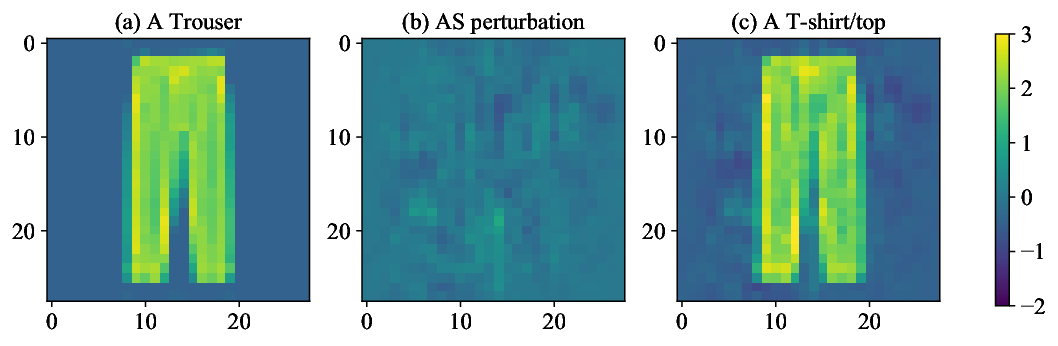
In Fig. 7, we plot one image from Fashion-MNIST and its perturbation by the active-subspace attack vector. The attacked image in Fig. 7 (c) still looks like a trouser for a human. However, the deep neural network misclassifies it as a t-shirt/top.
Figure 7: The effect of our attack method on one data sample in the Fashion-MNIST dataset. (a) A trouser from the original dataset. (b) An active-subspace perturbation vector with the norm equals to 5. (c) The perturbed sample is misclassified as a t-shirt/top by the deep neural network.
Figure 8: Universal adversarial attacks of VGG-19 on CIFAR-10 with respect to different -norm perturbations. (a)-(c): The training attack ratio, the testing attack ratio, and the CPU time in seconds for attacking one class dataset. (d)-(f): The results for attacking ten classes dataset together.
5.2.2 CIFAR-10
Next, we show the numerical results of attacking VGG-19 on CIFAR-10. Fig. 8 compares the active-subspace method compared with the baseline UAP and Gaussian random vectors.
The top figures show the results by the dataset in the first class (i.e., automobile), and the bottom figures show the results for all ten classes.
For both two cases, the proposed active-subspace attack can achieve 20% higher attack ratios while three times faster than UAP.
This is similar to the results in Fashion-MNIST because the active-subspace has a better ability to capture the global information.
Figure 9: Adversarial attack of VGG-19 on CIFAR-10 with different number of training samples. The -norm perturbation is fixed as 10. (a) The results of attacking the dataset from the first class; (b) The results of attacking the whole dataset with 10 classes.
We further show the effects of different number of training samples in Fig. 9.
When the number of samples is increased, the testing attack ratio is getting better.
In our numerical experiments, we set the number of samples as 100 for one-class experiments and 200 for all-classes experiments.
We continue to show the cross-model performance on four different ResNet networks and one VGG network.
We test the performance of the attack vector trained from one model on all other models.
Each row in Table 6 shows the results on the same deep neural network and each column shows the results of the same attack vector.
It shows that ResNet-20 is easier to be attacked compared with other models. This agrees with our intuition that a simple network structure such as ResNet-20 is less robust.
On the contrary, VGG-19 is the most robust.
The success of cross-model attacks indicates that these neural networks could find a similar feature.
Table 6: Cross-model performance for CIFAR-10
ResNet-20
ResNet-44
ResNet-56
ResNet-110
VGG-19
ResNet-20
91.35%
87.74%
86.28%
87.38%
81.16%
ResNet-44
84.75%
92.28%
87.03%
85.44%
83.44%
ResNet-56
83.63%
86.67%
90.15%
87.39%
84.38%
ResNet-110
71.02%
77.58%
74.19%
92.77%
77.32%
VGG-19
53.61%
59.74%
61.49%
66.29%
80.02%
5.2.3 CIFAR-100
Finally, we show the results on CIFAR-100 for both the first class (i.e., dolphin) and all classes.
Similar to Fashion-MNIST and CIFAR-10, Fig. 10 shows that active-subspace can achieve higher attack ratios than both UAP and Gaussian random vectors.
Further, compared with CIFAR-10, CIFAR-100 is easier to be attacked partially because it has more classes.
Figure 10: Results for universal adversarial attack for CIFAR-100 with respect to different -norm perturbations. (a)-(c): The results for attacking the dataset from the first class. (d)-(f): The results for attacking ten classes dataset together.
We summarize the results for different datasets in Table 7.
The second column shows the number of classes in the dataset.
In terms of testing attack ratio for the whole dataset, active-subspace achieves , , and higher attack ratios than UAP for Fashion-MNIST, CIFAR-10, and CIFAR-100, respectively.
In terms of the CPU time, active-subspace achieves , , and speedup than UAP on the Fashion-MNIST, CIFAR-10, and CIFAR-100, respectively.
Table 7: Summary of the universal attack for different datasets by the active-subspace compared with UAP and the random vector. The norm of perturbation is equal to 10.
Training Attack ratio
Testing Attack ratio
CPU time (s)
# Class
AS
UAP
Rand
AS
UAP
Rand
AS
UAP
Fashion-
1
100.0%
93.6%
1.8%
98.0%
91.3%
3.0%
0.15
5.49
MNIST
10
79.2%
51.5%
8.0%
73.3%
49.1%
12.3%
1.40
58.85
CIFAR-10
1
94.7%
79.8%
8.0%
84.5%
57.9%
10.6%
8.18
52.83
10
86.5%
65.9%
10.2%
74.9%
59.9%
17.0%
37.01
181.72
CIFAR-100
1
97.2%
87.9%
19.7%
92.1%
84.3%
37.9%
13.32
248.78
100
93.7%
86.5%
38.7%
83.5%
77.4%
52.0%
14.32
204.50
6 Conclusions and Discussions
This paper has analyzed deep neural networks by the active subspace method originally developed for dimensionality reduction of uncertainty quantification. We have investigated two problems: how many neurons and layers are necessary (or important) in a deep neural network, and how to generate a universal adversarial attack vector that can be applied to a set of testing data?
Firstly, we have presented a definition of “the number of active neurons” and have shown its theoretical error bounds for model reduction. Our numerical study has shown that many neurons and layers are not needed. Based on this observation, we have proposed a new network called ASNet by cutting off the whole neural network at a proper layer and replacing all subsequent layers with an active subspace layer and a polynomial chaos expansion layer.
The numerical experiments show that the proposed deep neural network structural analysis method can produce a new network with significant storage savings and computational speedup yet with little accuracy loss.
Our methods can be combined with existing model compression techniques (e.g., pruning, quantization and low-rank factorization) to develop compact deep neural network models that are more suitable for the deployment on resource-constrained platforms. Secondly, we have applied the active subspace to generate a universal attack vector that is independent of a specific data sample and can be applied to a whole dataset. Our proposed method can achieve a much higher attack ratio than the existing work [40] and enjoys a lower computational cost.
ASNet has two main goals: to detect the necessary neurons and layers, and to compress the existing network.
To fulfill the first goal, we require a pre-trained model because from Lemmas 4, and 5, the accuracy of the reduced model will approach that of the original one.
For the second task, the pre-trained model helps us to get a good estimation for the number of active neurons, a proper layer to cut off, and a good initialization for the active subspace layer and polynomial chaos expansion layer.
However, a pre-trained model is not required because we can construct ASNet in a heuristic way (as done in most DNN):
a reasonable guess for the number of active neurons and cut-off layer, and a random parameter initialization for the pre-model, the active subspace layer and the polynomial chaos expansion layer.
Acknowledgement
We thank the associate editor and referees for their valuable comments and suggestions.
References
[1]S. Abdoli, L. G. Hafemann, J. Rony, I. B. Ayed, P. Cardinal, and A. L.
Koerich, Universal adversarial audio perturbations, arXiv preprint
arXiv:1908.03173, (2019).
[2]A. Aghasi, A. Abdi, N. Nguyen, and J. Romberg, Net-trim: Convex
pruning of deep neural networks with performance guarantee, in Advances in
Neural Information Processing Systems, 2017, pp. 3177–3186.
[3]L. Armijo, Minimization of functions having lipschitz continuous
first partial derivatives, Pacific Journal of mathematics, 16 (1966),
pp. 1–3.
[4]S. Baluja and I. Fischer, Adversarial transformation networks:
Learning to generate adversarial examples, arXiv preprint arXiv:1703.09387,
(2017).
[5]M. Behjati, S.-M. Moosavi-Dezfooli, M. S. Baghshah, and P. Frossard, Universal adversarial attacks on text classifiers, in ICASSP 2019-2019 IEEE
International Conference on Acoustics, Speech and Signal Processing (ICASSP),
IEEE, 2019, pp. 7345–7349.
[6]E. G. Birgin, J. M. Martínez, and M. Raydan, Nonmonotone
spectral projected gradient methods on convex sets, SIAM Journal on
Optimization, 10 (2000), pp. 1196–1211.
[7]H. Cai, L. Zhu, and S. Han, ProxylessNAS: Direct neural
architecture search on target task and hardware, arXiv preprint
arXiv:1812.00332, (2018).
[8]N. Carlini and D. Wagner, Towards evaluating the robustness of
neural networks, in 2017 IEEE Symposium on Security and Privacy (SP), IEEE,
2017, pp. 39–57.
[9]P. G. Constantine, Active subspaces: Emerging ideas for dimension
reduction in parameter studies, vol. 2, SIAM, 2015.
[10]P. G. Constantine, E. Dow, and Q. Wang, Active subspace methods in
theory and practice: applications to kriging surfaces, SIAM Journal on
Scientific Computing, 36 (2014), pp. A1500–A1524.
[11]P. G. Constantine, M. Emory, J. Larsson, and G. Iaccarino, Exploiting active subspaces to quantify uncertainty in the numerical
simulation of the hyshot ii scramjet, Journal of Computational Physics, 302
(2015), pp. 1–20.
[12]M. Courbariaux, I. Hubara, D. Soudry, R. El-Yaniv, and Y. Bengio, Binarized neural networks: Training deep neural networks with weights and
activations constrained to +1 or-1, arXiv preprint arXiv:1602.02830,
(2016).
[13]C. Cui and Z. Zhang, Stochastic collocation with non-gaussian
correlated process variations: Theory, algorithms and applications, IEEE
Transactions on Components, Packaging and Manufacturing Technology, (2018).
[14]C. Cui and Z. Zhang, High-dimensional uncertainty quantification of
electronic and photonic ic with non-gaussian correlated process variations,
IEEE Transactions on Computer-Aided Design of Integrated Circuits and
Systems, (2019).
[15]L. Deng, P. Jiao, J. Pei, Z. Wu, and G. Li, Gxnor-net: Training deep
neural networks with ternary weights and activations without full-precision
memory under a unified discretization framework, Neural Networks, 100
(2018), pp. 49–58.
[16]G. K. Dziugaite, Z. Ghahramani, and D. M. Roy, A study of the effect
of jpg compression on adversarial images, arXiv preprint arXiv:1608.00853,
(2016).
[17]J. Frankle and M. Carbin, The lottery ticket hypothesis: Finding
sparse, trainable neural networks, arXiv preprint arXiv:1803.03635, (2018).
[18]T. Garipov, D. Podoprikhin, A. Novikov, and D. Vetrov, Ultimate
tensorization: compressing convolutional and FC layers alike, arXiv
preprint arXiv:1611.03214, (2016).
[19]R. Ge, R. Wang, and H. Zhao, Mildly overparametrized neural nets can
memorize training data efficiently, arXiv preprint arXiv:1909.11837,
(2019).
[20]R. G. Ghanem and P. D. Spanos, Stochastic finite element method:
Response statistics, in Stochastic Finite Elements: A Spectral Approach,
Springer, 1991, pp. 101–119.
[21]M. Ghashami, E. Liberty, J. M. Phillips, and D. P. Woodruff, Frequent directions: Simple and deterministic matrix sketching, SIAM Journal
on Computing, 45 (2016), pp. 1762–1792.
[22]I. J. Goodfellow, J. Shlens, and C. Szegedy, Explaining and
harnessing adversarial examples, arXiv preprint arXiv:1412.6572, (2014).
[23]A. Graves, S. Fernández, F. Gomez, and J. Schmidhuber, Connectionist temporal classification: labelling unsegmented sequence data
with recurrent neural networks, in Proceedings of the 23rd international
conference on Machine learning, ACM, 2006, pp. 369–376.
[24]N. Halko, P.-G. Martinsson, and J. A. Tropp, Finding structure with
randomness: Probabilistic algorithms for constructing approximate matrix
decompositions, SIAM review, 53 (2011), pp. 217–288.
[25]S. Han, H. Mao, and W. J. Dally, Deep compression: Compressing deep
neural networks with pruning, trained quantization and huffman coding, arXiv
preprint arXiv:1510.00149, (2015).
[26]C. Hawkins and Z. Zhang, Bayesian tensorized neural networks with
automatic rank selection, arXiv preprint arXiv:1905.10478, (2019).
[27]Y. He, J. Lin, Z. Liu, H. Wang, L.-J. Li, and S. Han, Amc: Automl
for model compression and acceleration on mobile devices, in Proceedings of
the European Conference on Computer Vision (ECCV), 2018, pp. 784–800.
[28]G. Hinton, O. Vinyals, and J. Dean, Distilling the knowledge in a
neural network, stat, 1050 (2015), p. 9.
[29]W. Hoeffding, Probability inequalities for sums of bounded random
variables, in The Collected Works of Wassily Hoeffding, Springer, 1994,
pp. 409–426.
[30]D. W. Hosmer Jr, S. Lemeshow, and R. X. Sturdivant, Applied logistic
regression, vol. 398, John Wiley & Sons, 2013.
[31]I. Jolliffe, Principal component analysis, in International
encyclopedia of statistical science, Springer, 2011, pp. 1094–1096.
[32]C. Kanbak, S.-M. Moosavi-Dezfooli, and P. Frossard, Geometric
robustness of deep networks: analysis and improvement, in Proceedings of the
IEEE Conference on Computer Vision and Pattern Recognition, 2018,
pp. 4441–4449.
[33]V. Khrulkov and I. Oseledets, Art of singular vectors and universal
adversarial perturbations, in Proceedings of the IEEE Conference on Computer
Vision and Pattern Recognition, 2018, pp. 8562–8570.
[34]D. P. Kingma and J. Ba, Adam: A method for stochastic optimization,
arXiv preprint arXiv:1412.6980, (2014).
[35]A. Krizhevsky, I. Sutskever, and G. E. Hinton, Imagenet
classification with deep convolutional neural networks, in Advances in
neural information processing systems, 2012, pp. 1097–1105.
[36]V. Lebedev, Y. Ganin, M. Rakhuba, I. Oseledets, and V. Lempitsky, Speeding-up convolutional neural networks using fine-tuned cp-decomposition,
arXiv preprint arXiv:1412.6553, (2014).
[37]D. R. Lide, Handbook of mathematical functions, in A Century of
Excellence in Measurements, Standards, and Technology, CRC Press, 2018,
pp. 135–139.
[38]L. Liu, L. Deng, X. Hu, M. Zhu, G. Li, Y. Ding, and Y. Xie, Dynamic
sparse graph for efficient deep learning, arXiv preprint arXiv:1810.00859,
(2018).
[39]Z. Liu, M. Sun, T. Zhou, G. Huang, and T. Darrell, Rethinking the
value of network pruning, arXiv preprint arXiv:1810.05270, (2018).
[40]S.-M. Moosavi-Dezfooli, A. Fawzi, O. Fawzi, and P. Frossard, Universal adversarial perturbations, in Proceedings of the IEEE conference
on computer vision and pattern recognition, 2017, pp. 1765–1773.
[41]S.-M. Moosavi-Dezfooli, A. Fawzi, and P. Frossard, Deepfool: a
simple and accurate method to fool deep neural networks, in Proceedings of
the IEEE conference on computer vision and pattern recognition, 2016,
pp. 2574–2582.
[42]P. Neekhara, S. Hussain, P. Pandey, S. Dubnov, J. McAuley, and
F. Koushanfar, Universal adversarial perturbations for speech
recognition systems, arXiv preprint arXiv:1905.03828, (2019).
[43]A. Novikov, D. Podoprikhin, A. Osokin, and D. P. Vetrov, Tensorizing
neural networks, in Advances in Neural Information Processing Systems, 2015,
pp. 442–450.
[44]S. Oymak and M. Soltanolkotabi, Towards moderate
overparameterization: global convergence guarantees for training shallow
neural networks, arXiv preprint arXiv:1902.04674, (2019).
[45]N. Papernot, P. McDaniel, S. Jha, M. Fredrikson, Z. B. Celik, and
A. Swami, The limitations of deep learning in adversarial settings, in
2016 IEEE European Symposium on Security and Privacy (EuroS&P), IEEE, 2016,
pp. 372–387.
[46]A. Romero, N. Ballas, S. E. Kahou, A. Chassang, C. Gatta, and Y. Bengio,
Fitnets: Hints for thin deep nets, arXiv preprint arXiv:1412.6550,
(2014).
[47]H. L. Royden, Real Analysis, Macmillan, 2010.
[48]T. M. Russi, Uncertainty quantification with experimental data and
complex system models, PhD thesis, UC Berkeley, 2010.
[49]T. N. Sainath, B. Kingsbury, V. Sindhwani, E. Arisoy, and B. Ramabhadran,
Low-rank matrix factorization for deep neural network training with
high-dimensional output targets, in IEEE international conference on
acoustics, speech and signal processing, 2013, pp. 6655–6659.
[50]S. Scardapane, D. Comminiello, A. Hussain, and A. Uncini, Group
sparse regularization for deep neural networks, Neurocomputing, 241 (2017),
pp. 81–89.
[51]M. Schmidt, E. Berg, M. Friedlander, and K. Murphy, Optimizing
costly functions with simple constraints: A limited-memory projected
quasi-newton algorithm, in Artificial Intelligence and Statistics, 2009,
pp. 456–463.
[52]A. C. Serban and E. Poll, Adversarial examples-a complete
characterisation of the phenomenon, arXiv preprint arXiv:1810.01185,
(2018).
[53]S. Shalev-Shwartz and T. Zhang, Accelerated proximal stochastic dual
coordinate ascent for regularized loss minimization, in International
Conference on Machine Learning, 2014, pp. 64–72.
[54]C. Szegedy, W. Zaremba, I. Sutskever, J. Bruna, D. Erhan, I. Goodfellow,
and R. Fergus, Intriguing properties of neural networks, arXiv
preprint arXiv:1312.6199, (2013).
[55]D. Xiu and G. E. Karniadakis, Modeling uncertainty in steady state
diffusion problems via generalized polynomial chaos, Computer methods in
applied mechanics and engineering, 191 (2002), pp. 4927–4948.
[56]D. Xiu and G. E. Karniadakis, The wiener–askey polynomial chaos for
stochastic differential equations, SIAM journal on scientific computing, 24
(2002), pp. 619–644.
[57]S. Ye, X. Feng, T. Zhang, X. Ma, S. Lin, Z. Li, K. Xu, W. Wen, S. Liu,
J. Tang, et al., Progressive DNN compression: A key to achieve
ultra-high weight pruning and quantization rates using ADMM, arXiv
preprint arXiv:1903.09769, (2019).
[58]T. Young, D. Hazarika, S. Poria, and E. Cambria, Recent trends in
deep learning based natural language processing, ieee Computational
intelligenCe magazine, 13 (2018), pp. 55–75.
[59]V. P. Zankin, G. V. Ryzhakov, and I. Oseledets, Gradient
descent-based D-optimal design for the least-squares polynomial
approximation, arXiv preprint arXiv:1806.06631, (2018).