Missing Value Imputation for Mixed Data via Gaussian CopulaCCS: Mathematics of computing Expectation maximizationCCS: Mathematics of computing Maximum likelihood estimationCCS: Computing methodologies Learning latent representations
Abstract.
Missing data imputation forms the first critical step of many data analysis pipelines. The challenge is greatest for mixed data sets, including real, Boolean, and ordinal data, where standard techniques for imputation fail basic sanity checks: for example, the imputed values may not follow the same distributions as the data. This paper proposes a new semiparametric algorithm to impute missing values, with no tuning parameters. The algorithm models mixed data as a Gaussian copula. This model can fit arbitrary marginals for continuous variables and can handle ordinal variables with many levels, including Boolean variables as a special case. We develop an efficient approximate EM algorithm to estimate copula parameters from incomplete mixed data. The resulting model reveals the statistical associations among variables. Experimental results on several synthetic and real datasets show the superiority of our proposed algorithm to state-of-the-art imputation algorithms for mixed data.
Keywords:
mixed data, ordinal data, Gaussian copula, missing values, imputation1. Introduction
Mixed data sets — those that include real, Boolean, and ordinal data — are a fixture of modern data analysis. Ordinal data is particularly common in survey datasets. For example, Netflix users rate movies on a scale of -. Social surveys may roughly bin respondents’ income or level of education as an ordinal variable, and ordinal Likert scales measure how strongly a respondent agrees with certain stated opinions. Binary variables may be considered a special case of an ordinal with two levels. Health data often contains ordinals that result from patient surveys or from coarse binning of continuous data into, e.g., cancer stages 0–IV or overweight vs obese patients. In all of these settings, missing data is endemic due to nonresponse and usually represents a large proportion of the dataset. Missing value imputation generally precedes other analysis, since most machine learning algorithms require complete observations. Imputation quality can strongly influence subsequent analysis.
To exploit the information in mixed data, imputation must account for the interaction between continuous and ordinal variables. Unfortunately, the joint distribution of mixed data can be complex. Existing parametric models are either too restrictive (Little and Rubin 2019) or require priori knowledge of the data distribution (Van Buuren and Oudshoorn 1999). Nonparametric methods, such as MissForest (Stekhoven and Bühlmann 2011), based on random forests, and imputeFAMD (Audigier et al. 2016), based on principal components analysis, tend to perform better. However, these two methods treat ordinal data as categorical, losing valuable information about the order. Further, they can only afford a limited number of categories.
It is tempting, but dangerous, to treat ordinal data with many levels as continuous. For example, the ordinal variable “Weeks Worked Last Year” from the General Social Survey dataset takes levels, but of the population worked either 0 or 52 weeks. Imputation that treats this variable as continuous (e.g., imputing with the mean) works terribly! As another example, consider using low rank matrix completion (Candès and Recht 2009; Recht et al. 2010; Keshavan et al. 2010; Mazumder et al. 2010) to impute missing entries in a movie rating datasets using a quadratic loss. This loss implicitly treats ratings encoded as – as numerical values, so the difference between ratings 3 and 4 is the same as that between ratings 4 and 5. Is this true? How could we tell?
A more sensible (and powerful) model treats ordinal data as generated by thresholding continuous data, as in (Rennie and Srebro 2005b; Rennie and Srebro 2005a). Figure 1 illustrates how correlations can by garbled by treating such data as continuous.
Our work builds on this intuition to model mixed data through the Gaussian copula model (Hoff et al. 2007; Liu et al. 2009; Fan et al. 2017; Feng and Ning 2019), which assumes the observed vector is generated by transforming each marginal of a latent normal vector. Under this model, we associate each variable (both ordinal and continuous) with a latent normal variable. Each ordinal level corresponds to an interval of values of the corresponding latent normal variable.
We propose an efficient EM algorithm to estimate a Gaussian copula model with incomplete mixed data and show how to use this model to impute missing values. Our method outperforms many state-of-the-art imputation algorithms for various real datasets including social survey data (whose columns have a varying number of ordinal levels), movie rating data (high missing ratio), music tagging data (binary data), etc. The proposed method has several advantages: the method has no hyper-parameters to tune and is invariant to coordinate-wise monotonic transformations in the data. Moreover, the fitted copula model is interpretable and can reveal statistical associations among variables, which is useful for social science applications. To our best knowledge, our proposed algorithm is the first frequentist approach to fit the Gaussian copula model with incomplete mixed data. Moreover, it is much faster than the existing Bayesian MCMC algorithm for the same model (Hoff et al. 2007); given the same time budget, our method produces substantially more accurate estimates.
1.1. RELATED WORK
Gaussian Copula for Mixed Data.
Modeling mixed data with the Gaussian copula model has been studied using both frequentist approaches (Fan et al. 2017; Feng and Ning 2019) and Bayesian approaches (Hoff et al. 2007; Murray et al. 2013; Cui et al. 2019). In (Murray et al. 2013; Cui et al. 2019), the authors further assume the latent normal vector is generated from a factor model. When all variables are ordinal, the Gaussian copula model is equivalent to the probit graphical model (Guo et al. 2015). However, all these previous work focuses on model estimation and theoretical properties of the estimators, and has overlooked the potential of these models for missing value imputation.
In fact, the frequentist parameter estimation methods proposed (Fan et al. 2017; Feng and Ning 2019; Guo et al. 2015) assume complete data; so these methods cannot perform imputation. Among Bayesian approaches, MCMC algorithms (Hoff et al. 2007; Murray et al. 2013; Cui et al. 2019) can fit the copula model with incomplete data and impute missing values. However, to use these models, one must select the number of factors for the models in (Murray et al. 2013; Cui et al. 2019). The sensitivity of these models to this parameter makes it a poor choice in practice for missing value imputation.
The implementation of (Hoff et al. 2007) is still the best method available to fit a Gaussian copula model for incomplete mixed data. Hollenbach et al. 2018 provides an important case study of this method for use in multiple imputation with an application to sociological data analysis. However, the method is slow and sensitive: the burn-in and sampling period must be carefully chosen for MCMC to converge, and many iterations are often required, so the method does not scale to even moderate size data, which limits its use in practice. Our model matches that of (Hoff et al. 2007), but our EM algorithm runs substantially faster.
Low rank matrix completion.
The generalized low rank models framework (Udell et al. 2016) handles missing values imputation for mixed data using a low rank model with appropriately chosen loss functions to ensure proper treatment of each data type. However, choosing the right loss functions for mixed data is challenging. A few papers share our motivation: for example, early papers by Rennie and Srebro (Rennie and Srebro 2005b; Rennie and Srebro 2005a) proposed a thresholding model to generate ordinals from real low rank matrices. Ganti et al. 2015 estimate monotonic transformations of a latent low rank matrix, but the method performs poorly in practice. Anderson-Bergman et al. 2018 posits that the mixed data are generated by marginally transforming the columns of the sum of a low rank matrix and isotropic Gaussian noise. While their marginal transformation coincides with the Gaussian copula model, their setup greatly differs in that it cannot identify the correlations between variables.
While low rank matrix completion methods scale well to large datasets, the low rank assumption is too weak to generalize well on long skinny datasets. Hence low rank methods tend to work well on “square-ish” datasets () (Udell and Townsend 2019), while the copula methods proposed here work better on long, skinny datasets.
2. Notation
Define for . Let be a random vector. We use to denote the subvector of with entries in subset . Let denote missing, observed continuous, and observed discrete (or ordinal) dimensions, respectively. The observed dimensions are , so .
Let be a matrix whose rows correspond to observations and columns to variables. We refer to the -th row, -th column, and -th element as and , respectively.
We say random variables and random vectors if their cumulative distribution functions (CDF) match. The elliptope is the set of correlation matrices.
3. Gaussian Copula
The Gaussian copula models complex multivariate distributions through transformations of a latent Gaussian vector. We call a random variable continuous when it is supported on an interval. We can match the marginals of any continuous random vector by applying a strictly monotone function to a random vector with standard normal marginals. Further, the required function is unique, as stated in Lemma 1.
Lemma 0.
Suppose is a continuous random vector with CDF for each coordinate , and is a random vector with standard normal marginals. Then there exists a unique elementwise strictly monotone function such that
| (1) |
where is the standard normal CDF.
All proofs appear in the supplementary materials. Notice the functions in Eq. 1 are strictly monotone, so their inverses exist. Define . Then has standard normal marginals, but the joint distribution of is not uniquely determined. The Gaussian copula model (or equivalently nonparanormal distribution (Liu et al. 2009)) further assumes is jointly normal.
Definition 0.
We say a continuous random vector follows the Gaussian copula with parameters and if there exists a correlation matrix and elementwise strictly monotone function such that for .
This model is semiparametric: it comprises nonparametric functions and parametric copula correlation matrix . The monotone establishes the mapping between observed and latent normal , while fully specifies the distribution of . Further, the correlation is invariant to elementwise strictly monotone transformation of . Concretely, if and where is elementwise strictly monotone, then . Thus the Gaussian copula separates the multivariate interaction from the marginal distribution .
When is strictly monotone, must be continuous. On the other hand, when is monotone but not strictly monotone, takes discrete values in the range of and can model ordinals. Thus for ordinals, will not be invertible. For convenience, we define a set-valued inverse . When the ordinal has range , Lemma 3 states that the only monotone function mapping continuous to is a cutoff function, defined for some parameter as
Lemma 0.
Suppose is an ordinal random variable with range and probability mass function and is a continuous random variable with CDF . Then is the unique monotone function that satisfies , where .
For example, in recommendation system we can think of the discrete ratings as obtained by rounding some ideal real valued score matrix. The rounding procedure amounts to apply a cutoff function. See Figure 2 for an example of cutoff function.
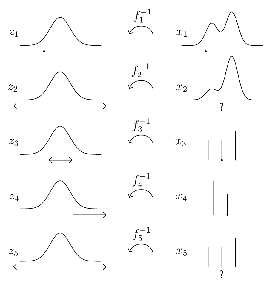
To extend the Gaussian copula to mixed data, we simply specify that is strictly monotone for and that is a cutoff function for . As before, the correlation remains invariant to elementwise strictly monotone transformations. The main difference is that while is a single number when is continuous, it is an interval when is discrete. See Figure 3 for illustration.
4. Imputation
So far we have introduced a very flexible model for mixed data. Our interest is to investigate missing value imputation under this model. Concretely, suppose the data matrix has rows and for . we first estimate and using observation and then impute missing values using , and observation .
In this section we first show how to impute the missing values with given estimates and . The estimation for appears in Section 5, and the estimation for appears in Section 6. The missing completely at random (MCAR) assumption is needed to consistently estimate . If the true is known, the missing at random (MAR) assumption suffices to consistently estimate . We discuss this issue further later in the paper.
For the latent normal vector satisfying , follows truncated normal distribution. Define for and for . In observed continuous dimensions , reduces to the point . In observed ordinal dimensions , lies in the Cartesian product of intervals . There is no constraint in missing dimension . It is natural to impute by mapping the conditional mean of through the marginals , summarized in Algorithm 1.
- (1)
Compute constraints .
- (2)
For ,
- •
Impute .
- •
Impute .
- •
While most applications require just a single imputation, multiple imputations are useful to describe the uncertainty due to imputation. Our method also supports multiple imputation: in step (2) of Algorithm 1, replace the conditional mean imputation with conditional sampling and then impute for each sample. The conditional sampling consists of two steps: (1) sample the truncated normal conditional on and ; (2) sample the normal conditional on and . Efficient sampling methods have been proposed (Pakman and Paninski 2014) for multivariate truncated normal distribution.
5. Monotonic Function Estimation
To map between and , we require both and . It is easier to directly estimate . For , we have , as shown in Eq. 1. While the true CDF is usually unavailable, it is natural to estimate it by the empirical CDF of on the observed entries, denoted as . We use the following estimator:
| (2) |
The scale constant ensures the output is finite. MCAR assumption guarantees the observed entries of are from the distribution of . Consider a case when MCAR is violated: an entry is observed if and only if it is smaller than a constant , then the observed entries are actually from the distribution :
Thus we assume MCAR in this section. This assumption may be relaxed to MAR or even missing not at random by carefully modeling or the missing mechanism. We leave that to our future work. Lemma 1 shows this estimator converges to in sup norm on the observed domain.
Lemma 0.
Suppose the continuous random variable with CDF and normal random variable satisfy for a strictly monotone . Given , , and , the inverse defined in Eq. 2 satisfies
for any in , where are constants depending on and .
For an ordinal variable with levels, . Since is determined by the probability mass function of , we may estimate cutoffs as a special case of Eq. 2 by replacing with its sample mean:
| (3) |
Lemma 2 shows that consistently estimates .
Lemma 0.
Suppose the ordinal random variable with probability mass function and normal random variable satisfy . Given samples , the cutoff estimate from Eq. 3 satisfies
for any in , where are constants depending on .
6. Copula Correlation Estimation
We first consider maximum likelihood estimation (MLE) for with complete continuous observation, then generalize the estimation method to incomplete mixed observation.
6.1. Complete Continuous Observations
We begin by considering continuous, fully observed data: . The density of the observed variable is
where , is the PDF of the normal vector with mean and covariance . The MLE of maximizes the likelihood function defined as:
| (4) |
over , where and is a universal constant (We omit here and later the constant arising from after the log transformation). Thus the MLE of is the sample covariance of . When we substitute by its empirical estimation in Eq. (2), the resulting covariance matrix of is still consistent and asymptotically normal under some regularity conditions (Tsukahara 2005), which justifies the use of our estimator . To simplify notation, we assume is known below.
For a Gaussian copula, notice is a correlation matrix, thus we update , where scales its argument to output a correlation matrix: for , . The obtained is still consistent and asymptotically normal.
6.2. Incomplete Mixed Observations
When some columns are ordinal and some data is missing, the Gaussian latent vector is no longer fully observed. We can compute the entries of corresponding to continuous data: . However, for ordinal data, is a Cartesian product of intervals; we only know that . The entries corresponding to missing observations, , are entirely unconstrained. Hence the latent matrix is only incompletely observed, and it is no longer possibly to simply compute its covariance.
We propose an expectation maximization (EM) algorithm to estimate for incomplete mixed observation. Proceeding in an iterative fashion, we replace unknown with their expectation conditional on observations and an estimate in the E-step, then in the M-step we update the estimate of as the conditional expectation of covaraince matrix:
| (5) |
Similar to the case of complete continuous data, we further scale the estimate to a correlation matrix. We first present the EM algorithm in Algorithm 2, then provide precise statements in Section 6.3. Computation details of Algorithm 2 appear in Section 6.4 and Section 6.5.
- (1)
E-step: Compute .
- (2)
M-step: .
- (3)
Scale to correlation matrix:
6.3. EM algorithm
We first write down the marginal density of observed values by integrating out the missing data. Since , there exist latent satisfying and . The likelihood of given observation is the integral over the latent Gaussian vector that maps to under the marginal . Hence the observed log likelihood we seek to maximize is:
| (6) |
where denote the submatrix of with rows and columns in . With known , MAR mechanism guarantees the maximizer of the likelihood in Eq. (6) shares the consistency and asymptotic normality of standard maximum likelihood estimate, according to the classical theory (Little and Rubin 2019, Chapter 6.2).
However, the maximizer has no closed form expression. Even direct evaluation of is challenging since it involves multivariate Gaussian integrals in a truncated region and the observed locations varies for different observations . Instead, the proposed EM algorithm is guaranteed to monotonically converge to a local maximizer according to classical EM theory (McLachlan and Krishnan 2007, Chapter 3).
Now we derive the proposed EM algorithm in detail. Suppose we know the values of the unobserved . Then the joint likelihood function is the same as in Eq. (4). Since the values of are unknown, we treat as latent variables and as observed variables. Substituting the joint likelihood function by its expected value given observations and an estimate :
EM theory (McLachlan and
Krishnan 2007, Chapter 3) guarantees the updated
improves the likelihood with ,
and that by iterating this update, we produce a sequence that converges monotonically to a local maximizer of . At the -th iteration, for the E step we compute to express in terms of . For the M step, we find . In practice, we resort to an approximation, as in (Guo et al. 2015). Notice that the unconstrained maximizer is . We update .
6.4. Conditional Expectation Computation
Suppressing index , we now show how to compute in Eq. (5). With , it suffices to compute the following terms:
- (1)
the conditional mean and covariance of observed ordinal dimensions .
- (2)
the conditional mean and covariance of missing dimensions .
- (3)
the conditional covariance between missing and observed ordinal dimensions .
We show that with the results from (1), we can compute (2) and (3). Computation for (1) is put in Sec 6.5.
Suppose we can know the ordinal values and thus . Conditional on , the missing dimensions follows normal distribution with mean . Further taking expectation of conditional on observation, we obtain
One can compute and similarly: deferring details to the supplement, we find
| (7) |
where has as its submatrix and elsewhere, has as its submatrix and elsewhere.
6.5. Approximating Truncated Normal Moments
Now it remains to compute and , which are the mean and covariance of a -dimensional normal truncated to , a Cartesian product of intervals. The computation involves multiple integrals of a nonlinear function and only admits a closed form expression when . Direct computational methods (BG and Wilhelm 2009) are very expensive and can be inaccurate even for moderate . Notice the computation needs to be done for each row at each EM iteration separately, thus sampling truncated normal distribution to evaluate the empirical moments (Pakman and Paninski 2014) is still expensive for large number of data points . Instead, we use a fast iterative method that scales well to large datasets, following (Guo et al. 2015).
Suppose all but one element of is known. Then we can easily compute the resulting one dimensional truncated normal mean: for , if is unknown and is known, let define the nonlinear function , parameterized by and , detailed in the supplement. We may also use to estimate if is known:
| (8) |
if is approximately linear. In other words, we can iteratively update the marginal mean of . At EM iteration , we conduct one iteration update with initial value from last EM iteration :
| (9) |
Surprisingly, one iteration update works well and more iterations do not bring significant improvement.
We use a diagonal approximation for :
we approximate as
for .
This approximation performs well when and are nearly independent given all observed information.
We approximate the diagonal entries
for using
a recursion similar to Eq. 9, detailed in the supplement.
We point out the estimated covariance matrix in Eq. (5) is the sum of the sample covariance matrix of the imputed using its conditional mean and the expected covariance brought by the imputation. The diagonal approximation only applies to the second term, while the first term is dense. Consequently, the estimator in Eq. (5) is dense and can fit a large range of covariance matrices. Empirical evidence indicates that our approximation even outperforms the MCMC algorithm without such diagonal approximation (Hoff et al. 2007), shown in Section 7.1.
6.6. Computation Cost
The complexity of each EM iteration is with observed entry ratio . The overall complexity is , where is the number of EM steps required for convergence. We found in most of our experiments. On a laptop with Intel-i5-3.1GHz Core and 8 GB RAM, it takes min for our algorithm to converge on a dataset with size and missing entries (generated as in Section 7.1 when ). Scaling our algorithm to large is important future work. However, our algorithm is usually faster than many start-of-the-art imputation algorithms for large small . Speed comparison on a dataset with size is shown in Section 7.3.
7. EXPERIMENTS
Our first experiment demonstrates that our method, Copula-EM, is able to estimate a well-specified Gaussian copula model faster than the MCMC method sbgcop (Hoff
et al. 2007; Hoff and Hoff 2018).
Our other experiments compare the accuracy of imputations produced by Copula-EM with
missForest (Stekhoven and
Bühlmann 2011), xPCA (Anderson-Bergman et al. 2018) and imputeFAMD (Audigier
et al. 2016), state-of-the-art nonparametric imputation algorithms for mixed data;
and the low rank matrix completion algorithms softImpute (Mazumder
et al. 2010)
and GLRM (Udell
et al. 2016), which scale to large datasets.
missForest is implemented with recommended default settings: maximum iterations and trees (Stekhoven 2011).
All other methods require selecting either the rank or the penalization parameter.
We select them through 5-fold cross validation (5CV), unless otherwise specified.
See the supplement for implementation details.
For real datasets, we report results from our Copula-EM but put that from sbgcop in the supplement,
since Copula-EM outperforms on all evaluation metrics
and converges substantially faster.
To measure the imputation error on columns in , we define a scaled mean absolute error (SMAE):
where are the imputed values and observed median for -th column, respectively. The estimator’s SMAE is smaller than if it outperforms column median imputation. For each data type, the SMAE can be computed on corresponding columns. To evaluate the estimated correlation, we use relative error , where is the estimated correlation matrix.
7.1. Synthetic Data
The first experiment compares the speed of the two algorithms to estimate Gaussian copula models: Copula-EM and sbgcop. Note Copula-EM is implemented in pure R, while the computational core of sbgcop is implemented in C. Hence further acceleration of Copula-EM is possible.
We generate 100 synthetic datasets with observations and variables from a well-specified Gaussian copula model with random generated (Qiu and Joe 2009). For each , first generate rows of as . Then generate using monotone such that have exponential distributions, are binary and are - ordinal.
We randomly remove of the entries of , train Copula-EM and sbgcop, and compute the imputation error on the held-out set. We plot the imputation accuracy and correlation estimation accuracy versus runtime of each algorithm in Figure 4. Copula-EM converges quickly, in about 25s, while sbgcop takes much longer and suffers high error at shorter times. Copula-EM estimates correlations and continuous imputations at convergence more accurately than sbgcop even when the latter algorithm is given times more runtime. Interestingly, Copula-EM recovers the correlation matrix better than sbgcop even asymptotically. These results demonstrate the impact of the approximate EM algorithm 6.5 compared to the (fully accurate) MCMC model of sbgcop: the approximation allows faster convergence, to an estimate of nearly the same quality.
For ordinal data imputation, Copula-EM reaches the same performance as sbgcop times faster. For binary data imputation, sbgcop is four times slower than Copula-EM at reaching the final performance of Copula-EM, but sbgcop outperforms Copula-EM given even more time. We conjecture that the drop in imputation accuracy of Copula-EM for binary data could be mitigated using multiple imputation (Little and Rubin 2019, Chapter 5.4), as outlined in Sec 4 by combining the imputations (using mean or median) into a single imputation to reduce the effect of approximating the truncated normal distribution.
The second experiment compares the imputation accuracy of Copula-EM and nonparametric algorithms. Using the same data generation mechanism, we randomly remove of the entries of . The optimal rank selected using 5CV is for xPCA and for imputeFAMD. Shown in Figure 5,Copula-EM substantially outperforms all nonparametric algorithms for all data types.
7.2. General Social Survey (GSS) Data
We chose variables with observations from GSS dataset in year 2014. of the entries are missing. The dataset consists of continuous (AGE) and ordinal variables with 2 to 48 levels. We investigate the imputation accuracy on five selected variables: INCOME, LIFE, HEALTH, CLASS11 1 Subjective class identification from lower to upper class and HAPPY. For each variable, we sample observation and divide them into folds. We mask one fold of only one variable as test data in each experiment. The selected rank is for both xPCA and imputeFAMD. We report the SMAE for each variable in Table 1. Our method performs the best for all variables. Further our method always performs better than median imputation. In contrast, the other three methods perform worse than median imputation for some variables. Our method also provides estimated variable correlation, which is usually desired in social survey study. We plot high correlations from the copula correlation matrix as a graph in Figure 6.
| Variable | Copula-EM | missForest | xPCA | imputeFAMD |
|---|---|---|---|---|
| CLASS | ||||
| LIFE | ||||
| HEALTH | ||||
| HAPPY | ||||
| INCOME |

7.3. MovieLens 1M Data
Recall our method scales cubicly in the number of variables. Hence for this experiment, we sample the subset of the MovieLens 1M data (Harper and Konstan 2016) consisting of the movies with at least ratings and all users who rate at least one of those movies. On this subset, of entries are missing. Under the time limit hour, we implement all algorithms but imputeFAMD. Copula-EM takes 9 mins and missForest takes 25 mins. These two methods have no parameters to tune. To select tuning parameters for other algorithms, we manually mask of the data for the test set and use the remaining data to train the model, and repeat 20 times. The selected rank using 5CV is for softImpute, for xPCA and for GLRM with bigger-vs-smaller loss. With the selected tuning parameter, low rank matrix completion methods are substantially faster. For example, softImpute only takes 33s. However, counting the additional time to select tuning parameters using 5CV, softImpute takes 16mins to select the penalization parameter with regularization path length 50, which is already more expensive than Copula-EM. Interestingly, the ranks selected are quite different even when the models perform similarly: GLRM chooses rank while softImpute chooses rank .
We report both mean absolute error (MAE) and RMSE in Table 2. Our method outperforms all others in both MAE and RMSE. This result is notable, because Copula-EM does not directly minimize MAE or RMSE, while softImpute directly minimizes RMSE. It also indicates Copula-EM does not overfit even with free parameters.
| Algorithm | MAE | RMSE |
|---|---|---|
| Column Median | ||
| Copula-EM | ||
| GLRM | ||
| softImpute | ||
| xPCA | ||
| missForest |
7.4. Music Auto-tagging: CAL500exp Data
The CAL500 expansion (CAL500exp) dataset (Wang et al. 2014) is an enriched version of the well-known CAL500 dataset (Turnbull et al. 2007). This dataset consists of 67 binary tags (including genre, mood and instrument, labeled by experts) to music fragments from songs. Music auto-tagging is a multi-label learning problem. A feature vector is usually computed first based on the music files and then a classifier is trained for each tag. This procedure is expensive and neglects the association among known labels. We treat this task as a missing data imputation problem and only use observed labels to impute unknown labels. This dataset is completely observed. We randomly remove some portions of the observed labels as a test set and repeat times. The selected optimal rank is for xPCA and for imputeFAMD. Shown in Table 3, Copula-EM performs the best in terms of SMAE. The superiority of Copula-EM over other algorithms substantially grows as the missing ratio increases. Moreover, Copula-EM yields very stable imputations: the standard deviation of its SMAE is imperceptibly small.
| Algorithm | missing | missing | missing |
|---|---|---|---|
| Copula-EM | |||
| missForest | |||
| imputeFAMD | |||
| xPCA |
7.5. More Ordinal Data and Mixed Data
We compare mixed data imputation algorithms on two more ordinal classification datasets22 2 Available at https://waikato.github.io/weka-wiki/datasets/, Lecturers Evaluation (LEV) and Employee Selection (ESL), and two more mixed datasets, German Breast Cancer Study Group (GBSG)33 3 Available at https://cran.r-project.org/web/packages/mfp/ and Restaurant Tips (TIPS)44 4 Available at http://ggobi.org/book/. Dataset descriptions appear in Table 4, and more details appear in the supplement. All datasets are completely observed.
For each dataset, we randomly remove entries as a test set and repeat times. For ordinal classification datasets, we evaluate the SMAE for the label and for the features, respectively. For mixed datasets, we evaluate the SMAE for ordinal dimensions and for continuous dimensions, respectively. We report results in Table 4. Our method outperforms the others in all but one setting, often by a substantial margin.
| Dataset | Size | Selected Rank | Type | Copula-EM | missForest | xPCA | imputeFAMD |
|---|---|---|---|---|---|---|---|
| ESL | 1 (xPCA) | Label | |||||
| 4 features, 1 label | 5 (imputeFAMD) | Feature | |||||
| LEV | 1 (xPCA) | Label | |||||
| 4 features, 1 label | 5 (imputeFAMD) | Feature | |||||
| GBSG | 2 (xPCA) | Ordinal | |||||
| 6 continuous, 4 ordinal | 2 (imputeFAMD) | Continuous | |||||
| TIPS | 2 (xPCA) | Ordinal | |||||
| 2 continuous, 5 ordinal | 6 (imputeFAMD) | Continuous |
8. SUMMARY AND DISCUSSION
In this paper, we proposed an imputation algorithm that models mixed data with a Gaussian copula model, together with an effective approximate EM algorithm to estimate the copula correlation with incomplete mixed data. Our algorithm has no tuning parameter and are easy to implement. Our experiments demonstrate the success of the proposed method. Scaling these methods to larger datasets (especially, with more columns), constitutes important future work.
We end by noting a few contrasts between the present approach and typical low rank approximation methods for data imputation. Low rank approximation constructs a latent simple (low rank) object and posits that observations are noisy draws from that simple latent object. In contrast, our approach uses a parametric, but full-dimensional, model for the latent object; observations are given by a deterministic function of the latent object. In other words, in previous work the latent object is exact and the observations are noisy; in our work, the latent object is noisy and the observations are exact. Which more faithfully models real data? As evidence, we might consider whether low rank models agree on the best rank to fit a given dataset. For example, on the MovieLens dataset: (1) The low rank matrix completion methods xPCA and GLRM, implemented using alternating minimization, select small optimal ranks (6 and 8), while softImpute, implemented using nuclear norm minimization, selects the much larger optimal rank . (2) Our algorithm outperforms all the low rank matrix completion methods we tested. These observations suggest the low rank assumption commonly used to fit the MovieLens dataset may not be fundamental, but may arise as a mathematical artifact (Udell and Townsend 2019). More supporting empirical results can be found in (Avron et al. 2012): the performance of softImpute keeps improving as the rank increases (up to ).
Acknowledgements.
We gratefully acknowledge support from NSF Awards IIS-1943131 and CCF-1740822, the ONR Young Investigator Program, DARPA Award FA8750-17-2-0101, the Simons Institute, Canadian Institutes of Health Research, and Capital One. We thank Clifford Anderson-Bergman and Tamara G. Kolda for help in understanding and implementing xPCA, Julie Josse for help in implementing imputeFAMD, and Yang Ning and Zhengze Zhou for helpful discussions. Special thanks go to Xiaoyi Zhu for help in producing Figure 3.References
- (1)
- Anderson-Bergman et al. (2018) Clifford Anderson-Bergman, Tamara G Kolda, and Kina Kincher-Winoto. 2018. XPCA: Extending PCA for a Combination of Discrete and Continuous Variables. arXiv preprint arXiv:1808.07510 (2018).
- Audigier et al. (2016) Vincent Audigier, François Husson, and Julie Josse. 2016. A principal component method to impute missing values for mixed data. Advances in Data Analysis and Classification 10, 1 (2016), 5–26.
- Avron et al. (2012) Haim Avron, Satyen Kale, Shiva Kasiviswanathan, and Vikas Sindhwani. 2012. Efficient and practical stochastic subgradient descent for nuclear norm regularization. arXiv preprint arXiv:1206.6384 (2012).
- BG and Wilhelm (2009) Manjunath BG and Stefan Wilhelm. 2009. Moments calculation for the double truncated multivariate normal density. Available at SSRN 1472153 (2009).
- Candès and Recht (2009) Emmanuel J Candès and Benjamin Recht. 2009. Exact matrix completion via convex optimization. Foundations of Computational mathematics 9, 6 (2009), 717.
- Cui et al. (2019) Ruifei Cui, Ioan Gabriel Bucur, Perry Groot, and Tom Heskes. 2019. A novel Bayesian approach for latent variable modeling from mixed data with missing values. Statistics and Computing 29, 5 (2019), 977–993.
- Dvoretzky et al. (1956) Aryeh Dvoretzky, Jack Kiefer, Jacob Wolfowitz, et al. 1956. Asymptotic minimax character of the sample distribution function and of the classical multinomial estimator. The Annals of Mathematical Statistics 27, 3 (1956), 642–669.
- Fan et al. (2017) Jianqing Fan, Han Liu, Yang Ning, and Hui Zou. 2017. High dimensional semiparametric latent graphical model for mixed data. Journal of the Royal Statistical Society: Series B (Statistical Methodology) 79, 2 (2017), 405–421.
- Feng and Ning (2019) Huijie Feng and Yang Ning. 2019. High-dimensional Mixed Graphical Model with Ordinal Data: Parameter Estimation and Statistical Inference. In The 22nd International Conference on Artificial Intelligence and Statistics. 654–663.
- Ganti et al. (2015) Ravi Sastry Ganti, Laura Balzano, and Rebecca Willett. 2015. Matrix completion under monotonic single index models. In Advances in Neural Information Processing Systems. 1873–1881.
- Guo et al. (2015) Jian Guo, Elizaveta Levina, George Michailidis, and Ji Zhu. 2015. Graphical models for ordinal data. Journal of Computational and Graphical Statistics 24, 1 (2015), 183–204.
- Harper and Konstan (2016) F Maxwell Harper and Joseph A Konstan. 2016. The movielens datasets: History and context. Acm transactions on interactive intelligent systems (tiis) 5, 4 (2016), 19.
- Hoff and Hoff (2018) Peter Hoff and Maintainer Peter Hoff. 2018. Package ‘sbgcop’. (2018).
- Hoff et al. (2007) Peter D Hoff et al. 2007. Extending the rank likelihood for semiparametric copula estimation. The Annals of Applied Statistics 1, 1 (2007), 265–283.
- Hollenbach et al. (2018) Florian M Hollenbach, Iavor Bojinov, Shahryar Minhas, Nils W Metternich, Michael D Ward, and Alexander Volfovsky. 2018. Multiple Imputation Using Gaussian Copulas. Sociological Methods & Research (2018), 0049124118799381.
- Keshavan et al. (2010) Raghunandan H Keshavan, Andrea Montanari, and Sewoong Oh. 2010. Matrix completion from noisy entries. Journal of Machine Learning Research 11, Jul (2010), 2057–2078.
- Kosorok (2008) Michael R Kosorok. 2008. Introduction to empirical processes and semiparametric inference. Springer.
- Little and Rubin (2019) Roderick JA Little and Donald B Rubin. 2019. Statistical analysis with missing data. Vol. 793. Wiley.
- Liu et al. (2009) Han Liu, John Lafferty, and Larry Wasserman. 2009. The nonparanormal: Semiparametric estimation of high dimensional undirected graphs. Journal of Machine Learning Research 10, Oct (2009), 2295–2328.
- Mazumder et al. (2010) Rahul Mazumder, Trevor Hastie, and Robert Tibshirani. 2010. Spectral regularization algorithms for learning large incomplete matrices. Journal of machine learning research 11, Aug (2010), 2287–2322.
- McLachlan and Krishnan (2007) Geoffrey McLachlan and Thriyambakam Krishnan. 2007. The EM algorithm and extensions. Vol. 382. John Wiley & Sons.
- Murray et al. (2013) Jared S Murray, David B Dunson, Lawrence Carin, and Joseph E Lucas. 2013. Bayesian Gaussian copula factor models for mixed data. J. Amer. Statist. Assoc. 108, 502 (2013), 656–665.
- Pakman and Paninski (2014) Ari Pakman and Liam Paninski. 2014. Exact hamiltonian monte carlo for truncated multivariate gaussians. Journal of Computational and Graphical Statistics 23, 2 (2014), 518–542.
- Qiu and Joe (2009) Weiliang Qiu and Harry Joe. 2009. clusterGeneration: random cluster generation (with specified degree of separation). R package version 1, 7 (2009), 75275–0122.
- Recht et al. (2010) Benjamin Recht, Maryam Fazel, and Pablo A Parrilo. 2010. Guaranteed minimum-rank solutions of linear matrix equations via nuclear norm minimization. SIAM review 52, 3 (2010), 471–501.
- Rennie and Srebro (2005a) Jasson DM Rennie and Nathan Srebro. 2005a. Fast maximum margin matrix factorization for collaborative prediction. In Proceedings of the 22nd international conference on Machine learning. ACM, 713–719.
- Rennie and Srebro (2005b) Jason DM Rennie and Nathan Srebro. 2005b. Loss functions for preference levels: Regression with discrete ordered labels. In Proceedings of the IJCAI multidisciplinary workshop on advances in preference handling. Kluwer Norwell, MA, 180–186.
- Stekhoven (2011) Daniel J Stekhoven. 2011. Using the missForest package. R package (2011), 1–11.
- Stekhoven and Bühlmann (2011) Daniel J Stekhoven and Peter Bühlmann. 2011. MissForest—non-parametric missing value imputation for mixed-type data. Bioinformatics 28, 1 (2011), 112–118.
- Tsukahara (2005) Hideatsu Tsukahara. 2005. Semiparametric estimation in copula models. Canadian Journal of Statistics 33, 3 (2005), 357–375.
- Turnbull et al. (2007) Douglas Turnbull, Luke Barrington, David Torres, and Gert Lanckriet. 2007. Towards musical query-by-semantic-description using the cal500 data set. In Proceedings of the 30th annual international ACM SIGIR conference on Research and development in information retrieval. 439–446.
- Udell et al. (2016) Madeleine Udell, Corinne Horn, Reza Zadeh, Stephen Boyd, et al. 2016. Generalized low rank models. Foundations and Trends® in Machine Learning 9, 1 (2016), 1–118.
- Udell and Townsend (2019) Madeleine Udell and Alex Townsend. 2019. Why are Big Data Matrices Approximately Low Rank? SIAM Journal on Mathematics of Data Science (SIMODS) 1, 1 (2019), 144–160. https://epubs.siam.org/doi/pdf/10.1137/18M1183480
- Vaart and Wellner (1996) Aad W Vaart and Jon A Wellner. 1996. Weak convergence and empirical processes: with applications to statistics. Springer.
- Van Buuren and Oudshoorn (1999) Stef Van Buuren and Karin Oudshoorn. 1999. Flexible multivariate imputation by MICE. Leiden: TNO.
- Wang et al. (2014) Shuo-Yang Wang, Ju-Chiang Wang, Yi-Hsuan Yang, and Hsin-Min Wang. 2014. Towards time-varying music auto-tagging based on CAL500 expansion. In 2014 IEEE International Conference on Multimedia and Expo (ICME). IEEE, 1–6.
Appendix A Computational Details
A.1. Details for Section 6.5
Denote the observation i.e. as . Since the task is to compute the marginal mean and variance of a multivariate truncated normal, we suppose here without loss of generality. For each , we use the law of total expectation by conditioning on first. Given , is univariate normal with mean and variance , truncated to the region , where the index means all dimensions but , i.e., . The region is an interval: . Here are three cases: (1) ; (2) ; (3) . The computation for all cases are similar. We take the first case as an example. First we introduce a lemma describing the first and second moments of a truncated univariate normal.
Lemma 0.
Suppose a univariate random variable . For constants , let and . Then the mean and variance of truncated to the interval are:
Plugging and into the above mean and variance formulas, we obtain the expression of defined in Section 6.5, and the univariate truncated normal variance , a nonlinear function , parameterized by and . Write down the formula for marginal variance conditional on observation:
We approximate the first term as . As for the second term, Guo et al. 2015 approximated it as based on . However, we found in practice simply dropping the second term performs better.
In summary, given an estimate and , for , we update and
. In other words, we update the conditional mean and variance of as the univariate truncated normal mean and variance with all other observed ordinal dimensions equal to their mean from last iteration, i.e. .
A.2. Details for Section 6.4
Given and , it suffices to compute and for and . Using the law of total expectation, we have:
Appendix B Supplement for Experiments
B.1. Implementation Details
For softImpute, we first center the rows and columns, then select the penalization parameter in the path from (rank ) to (rank ) with points. For GLRM, we use quadratic regularization on factor and ordinal regularization on factor. The model is fitted with SVD initialization and offest term. After a small grid search, we select the quadratic regularization parameter as where is the number of observed entries. Then the rank is selected through an exhaustive search. For xPCA and imputeFAMD, the rank is selected through an exhaustive search.
B.2. Results of sbgcop on Real Datasets
For GSS data, Copula-EM takes 24s, while sbgcop with iterations takes 87s, with imputation error: CALSS, ; LIFE, ; HEALTH, ; HAPPY, ; INCOME, .
For movielens data, Copula-EM takes 9 mins, while sbgcop with iterations takes 33 mins, with imputation error: MAE, ; RMSE, .
For CAL500exp data, Copula-EM takes 80s, while sbgcop with iterations takes 290s, with imputation error: for missing ratio; for missing ratio; for missing ratio.
For four small datasets used in Section 7.5, the time sbgcop with iterations takes is 2 times to 9 times (varying over datasets) of the time Copula-EM takes. The corresponding imputation error is: ESL label , feature ; LEV label , feature ; GBSG ordinal , continuous ; TIPS ordinal , continuous .
B.3. Datasets Description for Section 7.5
- ESL:
-
This dataset contains profiles of applicants for certain jobs. The recruiting company, based upon psychometric test results and interviews with the candidates, determined the values of the input attributes. The output is an overall score corresponding to the degree of fitness of the candidate.
- LEV:
-
This dataset contains lecturer evaluations. Students evaluate their lecturers according to four attributes such as oral skills and contribution to their professional/general knowledge. The output is an overall score of the lecturer’s performance.
- GBSG:
-
This dataset contains the information of women with breast cancer concerning the status of the tumours and the hormonal system of the patient.
- TIPS:
-
This dataset concerns the tips given to a waiter in a restaurant collected from customers. Recording variables contains the price of the meal, the tip amount and the conditions of the restaurant meal (number of guests, time of data, etc.).
Appendix C Proof of Lemmas
Proof of Lemma 1
Proof.
For any , if and only if (iff) and have the same CDF. For each , since exists for any strictly monotone , we can calculate the CDF of :
Then iff , equivalently, . ∎
Proof of Lemma 2
Proof.
It suffices to show for monotone function , iff with . Notice iff the range of is and for any . When , further define and . Since is continuous with CDF , it suffices to show:
When , has range . For , define and . Since , we have . Since is monotone, we have . Claim . If not, there exists satisfying . Since has range , can only be or . Equivalently or , which contradicts . Thus , ,
Thus we have .
∎
Proof of Lemma 3
Before we prove Lemma 3, we introduce the Dvoretzky-Kiefer-Wolfowitz inequality (Dvoretzky et al. 1956), also introduced in (Kosorok 2008).
The Dvoretzky-Kiefer-Wolfowitz Inequality 0.
For any i.i.d. sample with distribution , then when ,
Proof.
Applying the Dvoretzky-Kiefer-Wolfowitz inequality, for any , .
Take , . Further let , we have for . Then,
Since , we get . Adjusting the constants, for , we have
∎
Proof of Lemma 4
Before we prove Lemma 4, we introduce the Bretagnolle-Huber-Carol inequality introduced in (Vaart and Wellner 1996).
The Bretagnolle-Huber-Carol Inequality 0.
If the random vector is multinomially distributed with parameters and , then
Proof.
According to Lemma 2, the cutoff function is unique and . Define for , , and . Notice is multinomially distributed with parameters and , applying the Bretagnolle-Huber-Carol inequality, for any , with probability at least , . First for each , . Take , we have
When , we have . Further let , we have . Thus:
Let . Adjusting the constants, for , we have
∎