Isogeometric Analysis of the Gray-Scott Reaction-Diffusion Equations for Pattern Formation on Evolving Surfaces and Applications to Human Gyrification

The study of pattern formation is an active topic of reasearch that deals with qualitative and quantitative models for reproducing the many patterns found in the natural world, for instance in hair follicles [7], leaves [8], butterfly wings and mammalian coat markings [9]. Since Turing’s paper from $1952$ [29], a variety of reaction-diffusion (RD) systems have served as a standard model for how these patterns may arise naturally. So-called Turing Patterns formed in the concentration of the substrates subject to these RD-type systems show a great degree of resemblance with the stripes and spots as they appear in the many labyrinth-like patterns found in nature.
Pattern formation, resulting from RD-models, has been verified both experimentally [6] and computationally [5] and the field has broadened, greatly facilitated by computational simulation. A theoretical framework for the extension of RD-models to evolving surfaces, i.e., systems in which the two-dimensional geometry is a function of time, is presented in [10]. The evolution of the surface, in particular, may hereby be governed by the substrates on the surface.
Unfortunately, the underlying equations of such evolving RD-systems are often too complex to allow for an analytical treatment. This suggests the use of a numerical approach, typically one based on the principles of finite element analysis (FEA). The purpose of the present paper is to give an example of the discretization of the Grey-Scott RD-model on an evolving geometry, initially given by a spherical shell using the principles of Isogeometric Analysis [3], a variant of classical FEA. To this end, we adopt the Grey-Scott RD-based model for human brain development, proposed by Lefèvre et al. in [2] and present an IgA-based numerical scheme to tackle the underlying nonlinear equations. In the following, we present a short recap of models for human brain development and a motivation for the use of IgA as a numerical technique.
We note that the current model provides a description of human gyrification that is too simplistic from a biophysical point of view. As such, the presented work should be considered as a feasibility study for simulating pattern formation induced geometrical development of manifolds by the use of isogeometric analysis.

Neural development has become a topic of growing interest in the past decades. On the one hand healthy adult individuals exhibit qualitatively similar neural structures, on the other hand neural development exhibits a substantial degree of randomness, which is largely confirmed by the observation that even monozygotic twins exhibit significant anatomical differences [1]. Among other factors, this neural ‘fingerprint’ manifests itself mainly through the patterns formed in the neural folding and buckling process occurring naturally after the twentieth week of fetal development (see Figure 1).

The model proposed by [2] results in a complex system of equations that cannot be solved analytically. The main challenge is the fact that the chemical species affect the local parametric properties of the geometry which in turn affect the local expressions of the differential operators acting on the concentrations of the chemical species, leading to a highly nonlinear system. Complexity is further increased by the existence of nonlinear reaction terms. The authors of [2] present a numerical scheme that utilizes a finite-difference discretization in the temporal component, treating some terms implicitly and others explicitly, as well as a classical finite-element approach in the spatial components. The initial geometry is given by a triangularly tessellated spherical shell.
Growth is incorporated by extracting the magnitude of the velocity vector from the concentration of one of the chemical species at a triangle vertex, and a subsequent shift of its position in the direction of the local normal vector. On a tessellated surface, due to the non-smooth transition between adjacent triangles, the normal vector formally does not exist at the triangle vertices. The article does not explicitly state how the normal vector is computed but it is apparent that it is approximated by a weighed average of the normal vectors of the surrounding (planar) triangles. Within an implementation that is mainly focused on minimizing computational costs (in order to allow for a large amount of simulations), such an approach is reasonable.
Being able to construct smooth geometries would obviously constitute an improvement of above shortcoming since the normal vector is defined in every point on the geometry $\mathcal{M}$. To this end, the evident choice is to replace the classical finite-element approach with an approach based on isogeometric analysis (IgA). IgA aims to bridge the gap between classical FEA and the geometric modelling techniques from computer aided design (CAD). As such, the proposed approach, apart from some restrictions, allows for the reconstruction of the evolving surface by smooth B-spline basis functions of arbitrary polynomial order $p$ by using a spline-based mapping operator $\mathbf{s}:\Omega\rightarrow\mathcal{M}$. The geometry hereby inherits the regularity properties of the basis (locally up to $C^{p-1}$-regularity is possible) and the mapping operator becomes another unknown in the problem formulation. Numerically, we therefore treat it in the same way as the unknown concentrations on $\mathcal{M}$ and, by that, add more mathematical rigour to the scheme.
On the one hand, smoothness in the geometry will most-likely result in more appealing outcomes since non-smooth geometries are not realistic from a biological standpoint (we present more quantitative statements about accuracy in Section 3.4). Since the plausibility of a model can only be assessed by the quality of the results, we hereby regard the spline-based reconstruction of the evolving surface, made possible by an IgA-based numerical approach, as particularly important. We introduce an IgA-based numerical scheme in the hopes of adding more credibility to the model. Furthermore, smoothness allows for a (non-discrete) measure of curvature, which can subsequently serve as a local refinement criterion.
On the other hand, modelling an evolving geometry that is initially given by a spherical shell, (not approximated by a triangular tesselation), is challenging and requires a computational domain $\Omega$ that is comprised of several quadrilaterals. With a polynomial order of $p>1$, the computational costs per degree of freedom (DOF) of the proposed IgA-scheme are expected to be higher than in the FEA-approach proposed in [2] (unless $p=1$, in which case the costs are the same). Hence, this approach should be considered quality-oriented and may serve as inspiration for IgA-based numerical schemes of similar models for evolving surfaces.

We represent vectors and vector-valued functions utilizing bold-faced letters. The $n$-th entry of vector(-valued function) $\mathbf{r}$ is denoted by $r_{n}$ or $(\mathbf{r})_{n}$. Matrices are presented in square brackets. The $n$-th entry in the $m$-th column of matrix $[A]$ is denoted by $[A]_{n,m}$.
Let $\boldsymbol{\xi}=\left(\xi_{1},\ldots,\xi_{n}\right)^{T}$ and $\mathbf{x}=\left(x_{1},\ldots,x_{m}\right)^{T}$. We define the vector-by-vector derivative (Jacobian matrix) of $\mathbf{x}$ with respect to $\boldsymbol{\xi}$ as follows:

$$\frac{\partial\mathbf{x}}{\partial\boldsymbol{\xi}}=\begin{bmatrix}\frac{\partial x_{1}}{\partial\xi_{1}}&\frac{\partial x_{1}}{\partial\xi_{2}}&\ldots&\frac{\partial x_{1}}{\partial\xi_{n}}\\ \frac{\partial x_{2}}{\partial\xi_{1}}&\frac{\partial x_{2}}{\partial\xi_{2}}&\ldots&\frac{\partial x_{2}}{\partial\xi_{n}}\\ \vdots&\vdots&\ddots&\vdots\\ \frac{\partial x_{m}}{\partial\xi_{1}}&\frac{\partial x_{m}}{\partial\xi_{2}}&\ldots&\frac{\partial x_{m}}{\partial\xi_{n}}\end{bmatrix}.$$

(1.1)

In this manuscript, we will frequently work with finite-element bases. Usually the basis is denoted by $\Sigma=\{w_{1},\ldots,w_{N}\}$. When referring to elements of $\operatorname{span}\Sigma$, we allow for elements with weights from $\mathbb{R}^{n}$ with $n\neq 1$. The value of $n$ will always be clear from the context. We make frequent use of parameterizations. By $\mathbf{s}:\Omega\rightarrow\mathcal{M}$, with $\Omega\subset\mathbb{R}^{n}$ and $\mathcal{M}\subset\mathbb{R}^{m}$, $m\geq n$, we denote the mapping that parameterizes the geometry $\mathcal{M}$ with points from the parametric domain $\Omega$. ‘Local’ functions living on $\Omega$ are generally represented utilizing lower-case letters, for example $w:\Omega\rightarrow\mathbb{R}$. Functions living in parameter space $\Omega$ can be made ‘global’ by utilizing the inverse $\mathbf{s}^{-1}:\mathcal{M}\rightarrow\Omega$ of $\mathbf{s}$ and are generally represented by the corresponding upper-case letter, here: $W:\mathcal{M}\rightarrow\mathbb{R}$. Their relationship is given by

$\displaystyle W=w\circ\mathbf{s}^{-1},$

(1.2)

see Figure 3.

Let

$\displaystyle[J]=\frac{\partial\mathbf{s}}{\partial\boldsymbol{\xi}}$

(1.3)

denote the Jacobian matrix of the mapping $\mathbf{s}:\Omega\rightarrow\mathcal{M}$. By

$\displaystyle[g]=[J]^{T}[J],$

(1.4)

we denote the metric tensor associated with $\mathbf{s}$. For convenience, we introduce the short hand notation

$\displaystyle\sqrt{g}=\sqrt{\det[g]}$

(1.5)

for the canonical geometric factor induced by the metric.
Let $\mathbf{U}:\mathcal{M}\rightarrow T_{P}\mathcal{M}$ and $W:\mathcal{M}\rightarrow\mathbb{R}$, where $T_{P}\mathcal{M}$ denotes the tangent plane of $\mathcal{M}$ spanned by the column vectors of $[J]$. Similarly to scalar functions, the local counterparts of functions $\mathbf{U}:\mathcal{M}\rightarrow T_{P}\mathcal{M}$ receive the corresponding lower case letter. Their relationship is hence given by:

$\displaystyle\mathbf{U}=[J]\mathbf{u}.$

(1.6)

Hence, $[g]$ induces a canonical metric for vector-valued functions $U:\mathcal{M}\rightarrow T_{P}\mathcal{M}$ in local coordinates, since

$\displaystyle\mathbf{A}\cdot\mathbf{B}=\mathbf{a}^{T}[J]^{T}[J]\mathbf{b}=\mathbf{a}^{T}[g]\mathbf{b}\equiv\langle\mathbf{a},\mathbf{b}\rangle.$

(1.7)

Analogous to the standard divergence, the geometric divergence is defined as the negative adjoint of the surface gradient. This translates to local coordinates as follows:

$\displaystyle\int_{\Omega}w\left(\nabla_{\mathcal{M}}\cdot\mathbf{u}\right)\sqrt{g}\mathrm{d}\boldsymbol{\xi}$

$\displaystyle=-\int_{\Omega}\langle\nabla_{\mathcal{M}}w,\mathbf{u}\rangle\sqrt{g}\mathrm{d}\boldsymbol{\xi},$

(1.8)

for all functions $W$ that vanish on $\partial\mathcal{M}$ (compact support). The function that satisfies (1.8) is, in local coordinates, given by [15, p. 18]

$\displaystyle\nabla_{\mathcal{M}}\cdot\mathbf{u}$

$\displaystyle=\frac{1}{\sqrt{g}}\sum_{i=1}^{n}\frac{\partial}{\partial\xi_{i}}\left(\sqrt{g}u_{i}\right).$

(1.9)

In the remainder, we shall replace $\nabla_{\mathcal{M}}\rightarrow\nabla$ for convenience.
Similarly, the geometric gradient, in local coordinates, is given by [18, p. 62]

$\displaystyle\nabla w=[g]^{-1}\hat{\nabla}w,$

(1.10)

where $\hat{\nabla}$ denotes the nabla operator in local coordinates.
The Laplace-Beltrami operator, being the counterpart of the ordinary Laplace-operator, consequently satisfies $\Delta w\equiv\nabla\cdot\nabla w$. After some rearrangement, we find [4]

$\displaystyle\Delta w=\frac{1}{\sqrt{g}}\sum_{i,j=1}^{n}\frac{\partial}{\partial\xi_{i}}\left(\sqrt{g}g^{i,j}\frac{\partial}{\partial\xi_{j}}w\right),$

(1.11)

where the $g^{i,j}$ are the entries of $[g]^{-1}$.
The above expressions can be regarded as generalizations of the commonly-encountered differential operators on manifolds. As such, most of the operations involving partial integration that are commonly applied in FEA are still applicable. In particular

$\displaystyle\int_{\mathcal{M}}W\Delta U\mathrm{d}\mathbf{x}=\int_{\partial\mathcal{M}}W\nabla U\cdot\mathbf{N}_{\partial\mathcal{M}}\mathrm{d}l-\int_{\mathcal{M}}\nabla W\cdot\nabla U\mathrm{d}\mathbf{x},$

(1.12)

where $\mathbf{N}_{\partial\mathcal{M}}\in T_{P}\partial\mathcal{M}$ denotes the unit outward normal vector from the tangent plane of $\partial\mathcal{M}$.

As stated in Subsection 1.3, Isogeometric Analysis (IgA), first introduced by Hughes et al. in [3], is a numerical technique aimed at bridging the gap between the principles of CAD and FEA. As CAD-geometries (typically) come in the form of (B)-Spline- or NURBS-based [30] mapping operators $\mathbf{s}:\Omega\rightarrow\mathcal{M}$, the isoparametric principle, which states that the unknowns on the geometry $\mathcal{M}$ should be treated in the same way as $\mathcal{M}$ itself, lies at the heart of any IgA-based numerical simulation. To this end, the same NURBS basis used for the geometry is employed in the finite element analysis and the NURBS-based mapping operator $\mathbf{s}:\Omega\rightarrow\mathcal{M}$ is left unaltered, avoiding the need for tesselation. In the following, we present a brief recap of B-Splines, as well as spline-based surface mappings.
B-splines are piecewise-polynomial functions that can be constructed so as to satisfy various continuity properties at the places where the polynomial segments connect. Their properties are determined by the entries of the so-called knot vector

$\displaystyle\Xi=\{\xi_{1},\xi_{2},\ldots,\xi_{n+p+1}\}.$

(1.13)

The knot vector is a non-decreasing sequence of parametric values $\xi_{i}\subset[0,1]$ that determine the boundaries of the segments on which the spline-basis is polynomial. Selecting some polynomial order $p$, the $p$-th order spline-functions $N_{i,p}$ are constructed recursively, utilizing the relation (with $\tfrac{0}{0}\equiv 0$)

$\displaystyle N_{i,q}(\xi)=\frac{\xi-\xi_{i}}{\xi_{i+1}-\xi_{i}}N_{i,q-1}(\xi)+\frac{\xi_{i+q+1}-\xi}{\xi_{i+q+1}-\xi_{i+1}}N_{i+1,q-1}(\xi),$

(1.14)

starting from

$\displaystyle N_{i,0}=\left\{\begin{array}[]{ll}1&\text{if }\xi_{i}\leq\xi\leq\xi_{i+1}\\ 0&\text{otherwise}\end{array}\right.,$

and iterating until $q=p$. The support of basis function $N_{i,p}$ is given by the interval $\mathcal{I}_{i,p}=[\xi_{i},\xi_{i+p+1}]$ and the amount of continuous derivatives across knot $\xi_{j}$ is given by $p-m_{j}$, where $m_{j}$ is the multiplicity of $\xi_{j}$ in $\mathcal{I}_{i,p}$. In practice, $\xi_{1}=0$ is repeated $p+1$ times as well as $\xi_{n+p+1}$ such that $\xi_{1}=\ldots=\xi_{p+1}=0$ and $\xi_{n+1}=\ldots=\xi_{n+p+1}=1$. As a result, the resulting basis $\sigma=\{N_{1,p},\ldots,N_{n,p}\}$ forms a non-negative partition of unity on the entire parametric domain $[0,1]$, that is:

$\displaystyle\sum_{i=1}^{n}N_{i,p}(\xi)=1,$

(1.17)

with

$\displaystyle N_{i,p}(\xi)\geq 0,$

(1.18)

for all spline functions $N_{i,p}$ [3]. Figure 4 shows the $p=3$ B-spline basis resulting from the knot vector

$\displaystyle\Xi=\left\{0,0,0,0,\tfrac{1}{7},\tfrac{2}{7},\tfrac{3}{7},\tfrac{4}{7},\tfrac{5}{7},\tfrac{6}{7},1,1,1,1\right\}.$

(1.19)

We can formulate the system comprised of substrates $U$ and $V$ and geometry $\mathcal{M}_{t}$ parameterized by $\mathbf{s}(\boldsymbol{\xi},t)$ as a system of equations in local coordinates

$\displaystyle\partial_{t}\begin{bmatrix}u\\ v\\ \mathbf{s}\end{bmatrix}$

$\displaystyle=\begin{bmatrix}-u\partial_{t}\left(\ln\sqrt{g_{t}}\right)+d_{1}\Delta_{t}u+F(1-u)-uv^{2}\\ -v\partial_{t}\left(\ln\sqrt{g_{t}}\right)+d_{2}\Delta_{t}v-(F+H)v+uv^{2}\\ Kv\mathbf{n}\end{bmatrix},$

(3.2)

with

$\displaystyle\mathbf{n}(\mathbf{s})$

$\displaystyle=\frac{1}{\left\|\frac{\partial\mathbf{s}}{\partial\xi}\times\frac{\partial\mathbf{s}}{\partial\eta}\right\|}\left(\frac{\partial\mathbf{s}}{\partial\xi}\times\frac{\partial\mathbf{s}}{\partial\eta}\right).$

(3.3)

Defining

$\displaystyle\mathbf{u}$

$\displaystyle=\begin{bmatrix}u&v&\mathbf{s}\end{bmatrix}^{T}$

(3.4)

and

$\displaystyle\mathbf{f}(\mathbf{u})$

$\displaystyle=\begin{bmatrix}-u\partial_{t}\left(\ln\sqrt{g_{t}}\right)+d_{1}\Delta_{t}u+F(1-u)-uv^{2}\\ -v\partial_{t}\left(\ln\sqrt{g_{t}}\right)+d_{2}\Delta_{t}v-(F+H)v+uv^{2}\\ Kv\mathbf{n}\end{bmatrix},$

(3.5)

the system of equations can be written as:

$\displaystyle\partial_{t}\mathbf{u}$

$\displaystyle=\mathbf{f}(\mathbf{u}).$

(3.6)

The individual components of $\mathbf{f}(\mathbf{u})$ shall be referred to as $f_{u},f_{v}$ and $f_{\mathbf{s}}$. Note that $f_{\mathbf{s}}$ is itself a vector-valued function.
We integrate both sides of (3.6):

		$\displaystyle\int_{t^{k}}^{t^{k+1}}\partial_{t}\mathbf{u}\mathrm{d}t$	$\displaystyle{}=$	$\displaystyle\int_{t^{k}}^{t^{k+1}}\mathbf{f}(\mathbf{u})\mathrm{d}t$
	$\displaystyle\implies\quad$	$\displaystyle\mathbf{u}\left(t^{k+1}\right)-\mathbf{u}\left(t^{k}\right)$	$\displaystyle=$	$\displaystyle\int_{t^{k}}^{t^{k+1}}\mathbf{f}(\mathbf{u})\mathrm{d}t.$		(3.7)

Before proceeding to the discretization, we define $\mathbf{u}^{k}$ as the approximation of $\mathbf{u}\left(t^{k}\right)$, resulting from the discretized scheme.
The right-hand-side integral of (3.1) is approximated by a mixed implicit / explicit (IMEX) quadrature. Defining $h_{k}=t^{k+1}-t^{k}$, we utilize:

$\displaystyle\int_{t^{k}}^{t^{k+1}}\mathbf{f}(u,v,\mathbf{s})\mathrm{d}t$

$\displaystyle\simeq h_{k}\left[\mathbf{g}(u^{k+1},v^{k+1},\mathbf{s}^{k},\mathbf{s}^{k-1})+\mathbf{h}(u^{k},v^{k},v^{k+1},\mathbf{s}^{k})\right],$

(3.8)

Here,

$\displaystyle\mathbf{g}(u^{k+1},v^{k+1},\mathbf{s}^{k},\mathbf{s}^{k-1})$

$\displaystyle=\begin{bmatrix}\begin{aligned} -&u^{k+1}\partial_{t}^{h}\left(\ln\sqrt{g_{k}}\right)+d_{1}\Delta_{k}u^{k+1}-Fu^{k+1}\\ -&v^{k+1}\partial_{t}^{h}\left(\ln\sqrt{g_{k}}\right)+d_{2}\Delta_{k}v^{k+1}-(F+H)v^{k+1}\end{aligned}\\ \mathbf{0}\end{bmatrix}$

(3.9)

and

$\displaystyle\mathbf{h}(u^{k},v^{k},v^{k+1},\mathbf{s}^{k})$

$\displaystyle=\begin{bmatrix}\begin{aligned} -&u^{k}\left(v^{k}\right)^{2}+F\\ &u^{k}\left(v^{k}\right)^{2}\end{aligned}\\ K\mathbf{n}^{k}v^{k+1}\end{bmatrix},$

(3.10)

with $\mathbf{n}^{k}=\mathbf{n}(\mathbf{s}^{k})$, $\Delta_{k}\equiv\Delta_{t^{k}}$ and $\sqrt{g_{k}}\equiv\sqrt{g_{t^{k}}}$.
The expression $\partial_{t}^{h}\left(\ln\sqrt{g_{k}}\right)$ represents the time-discretization of $\partial_{t}\left(\ln\sqrt{g_{k}}\right)$:

$\displaystyle\partial_{t}^{h}\left(\ln\sqrt{g_{k}}\right)$

$\displaystyle=\frac{\ln\sqrt{g_{k}}-\ln\sqrt{g_{k-1}}}{h_{k-1}}.$

(3.11)

We utilize a backward-difference scheme to avoid having to include $\sqrt{g_{k+1}}$ which is unknown at time-instance $t=t^{k}$.
We cast the discretized system into the form

$\displaystyle\mathbf{L}(\mathbf{u}^{k+1})$

$\displaystyle=\mathbf{u}^{k}+h^{k}\mathbf{h}\left(u^{k},v^{k},v^{k+1}\right),$

(3.12)

where

$\displaystyle\mathbf{L}\left(\mathbf{u}^{k+1}\right)$

$\displaystyle=\begin{bmatrix}\left\{h_{k}\left[\partial_{t}^{h}\left(\ln\sqrt{g_{k}}\right)-d_{1}\Delta_{k}+F\right]+1\right\}u^{k+1}\\ \left\{h_{k}\left[\partial_{t}^{h}\left(\ln\sqrt{g_{k}}\right)-d_{2}\Delta_{k}+F+H\right]+1\right\}v^{k+1}\\ \mathbf{s}^{k+1}\end{bmatrix}.$

(3.13)

As before, the individual components of $\mathbf{L},\mathbf{g}$ and $\mathbf{h}$ are referred to utilizing $u$, $v$ and $\mathbf{s}$ subscripts. Note that $\mathbf{L}$ is linear in ${\bf u}$, and that each component of $\mathbf{L}(\mathbf{u}^{k+1})$ only depends on the corresponding component in $\mathbf{u}^{k+1}$.

We first multiply equation (3.12) by a test-function $W:\mathcal{M}_{k}\rightarrow\mathbb{R}$ and integrate over $\mathcal{M}_{k}$. For the sake of brevity, we utilize $\mathrm{d}\Omega_{k}\equiv\sqrt{g_{k}}\mathrm{d}\boldsymbol{\xi}$. Note that integrals over $\mathcal{M}_{k}$ are locally reformulated in terms of integrals over the hollow cube $\Omega$. The additional pull-back from the faces of $\Omega$ into the reference domain is omitted for the sake of simplicity. We have:

		$\displaystyle\int_{\mathcal{M}_{k}}W\mathbf{L}_{u}(U^{k+1})\mathrm{d}\mathbf{x}=\int_{\mathcal{M}_{k}}W\left[U^{k}+h_{k}\mathbf{h}_{u}\left(U^{k},V^{k}\right)\right]\mathrm{d}\mathbf{x}$
	$\displaystyle\iff\quad$	$\displaystyle\begin{aligned} h_{k}d_{1}\int_{\Omega}\langle\nabla_{k}w,\nabla_{k}u^{k+1}\rangle_{g_{k}}\mathrm{d}\Omega_{k}&+\int_{\Omega}w\left[\left(\partial_{t}^{h}\left(\ln\sqrt{g_{k}}\right)+F\right)h_{k}+1\right]u^{k+1}\mathrm{d}\Omega_{k}\\ &=\int_{\Omega}w\left[u^{k}+h_{k}\mathbf{h}_{u}\left(u^{k},v^{k}\right)\right]\mathrm{d}\Omega_{k},\end{aligned}$		(3.14)

where we have made use of integration by parts, see equation (1.12), in conjunction with the assumption that $\mathcal{M}_{k}$ is a manifold without a boundary.
Similarly, we obtain:

		$\displaystyle\int_{\mathcal{M}_{k}}W\mathbf{L}_{v}(V^{k+1})\mathrm{d}\mathbf{x}=\int_{\mathcal{M}_{k}}W\left[V^{k}+h_{k}\mathbf{h}_{v}\left(U^{k},V^{k}\right)\right]\mathrm{d}\mathbf{x}$
	$\displaystyle\iff\quad$	$\displaystyle\begin{aligned} h_{k}d_{2}\int_{\Omega}\langle\nabla_{k}w,\nabla_{k}v^{k+1}\rangle_{g_{k}}\mathrm{d}\Omega_{k}&+\int_{\Omega}w\left[\left(\partial_{t}^{h}\left(\ln\sqrt{g_{k}}\right)+F+H\right)h_{k}+1\right]v^{k+1}\mathrm{d}\Omega_{k}\\ &=\int_{\Omega}w\left[v^{k}+h_{k}\mathbf{h}_{v}\left(u^{k},v^{k}\right)\right]\mathrm{d}\Omega_{k}.\end{aligned}$		(3.15)

As a next step, we introduce a local basis $\Sigma=\{w_{1},\ldots,w_{N}\}$. In equations (3.2) and (3.2), we successively replace $w$ by $w_{i},\enskip i=1,\ldots,N$ and we approximate $u^{k},v^{k}$ and $\mathbf{s}^{k}$ by elements from $\operatorname{span}\Sigma$,

$\displaystyle u^{k}$

$\displaystyle=\sum_{i=1}^{n}c_{i}^{k}w_{i},\quad v^{k}=\sum_{i=1}^{N}d_{i}^{k}w_{i}\quad\text{and}\quad\mathbf{s}^{k}=\sum_{i=1}^{N}\mathbf{e}_{i}^{k}w_{i}.$

(3.16)

Introducing $[A]$, $[B]$, $[D]$, $\mathbf{f}^{r}$ and $\mathbf{w}$ with

		$\displaystyle[A]_{i,j}=\int_{\Omega}w_{i}w_{j}\mathrm{d}\Omega_{k},\quad[D]_{i,j}=\int_{\Omega}\langle\nabla_{k}w_{i},\nabla_{k}w_{j}\rangle_{g_{k}}\mathrm{d}\Omega_{k},$
		$\displaystyle[B]_{i,j}=\int_{\Omega}w_{i}w_{j}\partial_{t}^{h}\left(\ln\sqrt{g_{k}}\right)\mathrm{d}\Omega_{k},\quad(\mathbf{f}^{r})_{i}=\int_{\Omega}w_{i}u^{k}\left(v^{k}\right)^{2}\mathrm{d}\Omega_{k}\text{ and }(\mathbf{w})_{i}=\int_{\Omega}w_{i}\mathrm{d}\Omega_{k},$		(3.17)

we can construct a system of equations for $\mathbf{c}^{k+1}=\left(c_{1}^{k+1},\ldots,c_{N}^{k+1}\right)^{T}$ and $\mathbf{d}^{k+1}=\left(d_{1}^{k+1},\ldots,d_{N}^{k+1}\right)^{T}$. They satisfy:

$\displaystyle\left\{[A](1+h_{k}F)+d_{1}h_{k}[D]+h_{k}[B]\right\}\mathbf{c}^{k+1}$

$\displaystyle=h_{k}F\mathbf{w}-h_{k}\mathbf{f}^{r}+[A]\mathbf{c}^{k},$

(3.18)

and

$\displaystyle\left\{[A](1+h_{k}(F+H))+d_{2}h_{k}[D]+h_{k}[B]\right\}\mathbf{d}^{k+1}$

$\displaystyle=h_{k}\mathbf{f}^{r}+[A]\mathbf{d}^{k}.$

(3.19)

Note that, strictly speaking, the matrices and vectors from equation (3.2) should receive a time-superscript which has been omitted for the sake of brevity.
After systems (3.18) and (3.19) have been solved at time-instance $t^{k+1}$, we are in the position to update the geometry. Equations (3.12) and (3.13) suggest that we should update according to the relation

$\displaystyle\mathbf{s}^{k+1}$

$\displaystyle=\mathbf{s}^{k}+h_{k}Kv^{k+1}\mathbf{n}^{k}.$

(3.20)

We solve (3.20) in the weak sense, leading to

$\displaystyle\int_{\Omega}w_{i}\mathbf{s}^{k+1}_{j}\mathrm{d}\Omega_{k}=\int_{\Omega}w_{i}\left(\mathbf{s}^{k}+h_{k}Kv^{k+1}\mathbf{n}^{k}\right)_{j}\mathrm{d}\Omega_{k}\quad\forall(w_{i},j)\in\Sigma\times\{1,2,3\},$

(3.21)

finalizing the iteration.

Assuming that $\mathbf{s}^{k}$ parameterizes a boundaryless geometry for all $k$, there are no essential spatial boundary conditions for functions $U:\mathcal{M}_{k}\rightarrow\mathbb{R}$. There do, however, exist requirements for functions $u:\Omega\rightarrow\mathbb{R}$ and some initial condition

$\displaystyle\mathbf{u}(t=0)$

$\displaystyle=\mathbf{i},$

(3.22)

The projections of the components of $\mathbf{u}(t=0)$ onto the basis $\Sigma$ become the first iterates $u^{0}$, $v^{0}$ and $\mathbf{s}^{0}$ that jointly form the discretized initial condition.
The requirements we have to impose on functions $u:\Omega\rightarrow\mathbb{R}$ follow from the requirement that any $U:\mathcal{M}_{k}\rightarrow\mathbb{R}$ must be a function on $\mathcal{M}_{k}$ and hence single-valued on $\mathcal{M}_{k}$. In order to be compatible with the finite-element discretization, we have to furthermore require that functions $U:\mathcal{M}_{K}\rightarrow\mathbb{R}$ satisfy $U\in H^{1}(\mathcal{M}_{k})$. Clearly, thanks to the well-behavedness of the metric induced by the mapping (see Section 1.5), the boundedness of first-order derivatives induced by $\nabla_{k}$ are conditional on the boundedness of first order derivatives in local coordinates. As such, a sufficient condition for this requirement is straightforwardly translated to local functions living in $\Omega$:

$\displaystyle u\in H^{1}(\Omega)\implies U\in H^{1}(\mathcal{M}_{k}).$

(3.23)

As we shall see, this is a critical requirement especially on shared edges / vertices of the various patches under the mapping $\mathbf{s}^{k}$. We enforce requirement (3.23) directly on the local basis functions $w_{i},\enskip i=1,\ldots,N$ such that the global counterpart $U$ of any $u\in\operatorname{span}\Sigma$ satisfies $U\in H^{1}(\mathcal{M}_{k})$ by default.
Let $\Omega_{i},\enskip i=1,\ldots,6$ refer to the various faces of $\Omega$. The connectivities of the various patches on $\mathcal{M}_{k}$ follow trivially from the connectivity of the $\Omega_{i}$ on $\Omega$. Hence there are pairs of faces $(\Omega_{i},\Omega_{j})$ for which $\partial\Omega_{i}\cap\partial\Omega_{j}\neq\emptyset$. For functions $U:\mathcal{M}_{k}\rightarrow\mathbb{R}$, we have to impose:

$\displaystyle\left\{\begin{array}[]{ll}u&\in C^{0}(\Omega)\\ u|_{\Omega_{i}}&\in H^{1}(\Omega_{i}),\enskip\forall i\in\{1,\ldots,6\}\end{array}\right..$

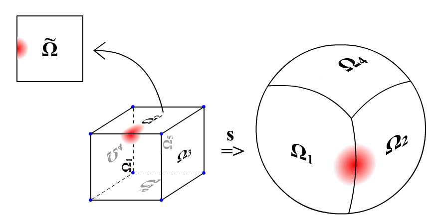
With condition (3.3) in mind, it becomes apparent that we can construct valid bases from the patchwise discontinuous bases $\Sigma_{i},i\in\{1,\ldots,6\}$ living on the $\Omega_{i}$ with appropriate degree of freedom coupling. We will assume that, upon pull-back into the reference domain, the $\Sigma_{i}$ constitute spline-bases with identical open and uniform knot vectors in both coordinate directions. As such, the bases are compatible at shared edges / vertices in the sense that oppositely-faced boundary-functions can be combined into one function that is compatible with (3.23) (see Figure 5). Besides the pairs of functions that need to be coupled on either side in the interior of shared edges, it is worth noting that the cube has eight extraordinary vertices where three functions need to be coupled (see Figure 6).

In equation (3.8), we introduced the temporal discretization of the right-hand side term $\mathbf{f}(u,v,\mathbf{s})$ with

	$\displaystyle\int_{t^{k}}^{t^{k+1}}\mathbf{f}_{u}\mathrm{d}t$	$\displaystyle\simeq h_{k}\left[-u^{k+1}\partial_{t}^{h}\left(\ln\sqrt{g_{k}}\right)+d_{1}\Delta_{k}u^{k+1}-Fu^{k+1}-u^{k}\left(v^{k}\right)^{2}+F\right]$
	$\displaystyle\int_{t^{k}}^{t^{k+1}}\mathbf{f}_{v}\mathrm{d}t$	$\displaystyle\simeq h_{k}\left[-v^{k+1}\partial_{t}^{h}\left(\ln\sqrt{g_{k}}\right)+d_{1}\Delta_{k}v^{k+1}-(F+H)v^{k+1}+u^{k}\left(v^{k}\right)^{2}\right]$
	$\displaystyle\int_{t^{k}}^{t^{k+1}}\mathbf{f}_{\mathbf{s}}\mathrm{d}t$	$\displaystyle\simeq h_{k}K\mathbf{n}^{k}v^{k+1}.$		(3.26)

The scheme can be regarded as a mixed implicit / explicit (IMEX [11]) scheme with the additional feature that $\mathbf{s}^{k-1}$ is present in $\partial_{t}^{h}\left(\ln\sqrt{g_{k}}\right)$. The local truncation errors $\tau_{k}$ for the individual components of the temporal discretization are given by:

	$\displaystyle\tau_{k}(\mathbf{f}_{u})$	$\displaystyle=\mathcal{O}(h_{k})+\mathcal{O}(h_{k-1})$
	$\displaystyle\tau_{k}(\mathbf{f}_{v})$	$\displaystyle=\mathcal{O}(h_{k})+\mathcal{O}(h_{k-1})$
	$\displaystyle\tau_{k}(\mathbf{f}_{\mathbf{s}})_{i}$	$\displaystyle=\mathcal{O}(h_{k}).$		(3.27)

The global error is of the same order [12].
In the following, we investigate the properties of the scheme introduced in Section 3.2, in particular symmetry and coercivity. The weak form leads to a left hand side operator of the form:

$\displaystyle\mathbf{A}^{k}(W,\mathbf{U}^{k+1})=\int_{\mathcal{M}_{k}}W\mathbf{L}(\mathbf{U}^{k+1})\mathrm{d}\mathbf{x}.$

(3.28)

As each component of $\mathbf{L}(\mathbf{U}^{k+1})$ only depends on the corresponding component in $\mathbf{U}^{k+1}$, the analysis can be carried out component-wisely. In equation (3.2), we derived:

$\displaystyle\mathbf{A}^{k}_{u}(U,V)=h_{k}d_{1}\int_{\Omega}\langle\nabla_{k}u,\nabla_{k}v\rangle_{g_{k}}\mathrm{d}\Omega_{k}$

$\displaystyle+\int_{\Omega}u\left[\left(\partial_{t}^{h}\left(\ln\sqrt{g_{k}}\right)+F\right)h_{k}+1\right]v\mathrm{d}\Omega_{k}.$

(3.29)

Clearly, $\mathbf{A}^{k}_{u}(U,V)$ is symmetric. Furthermore, we have:

	$\displaystyle\mathbf{A}^{k}_{u}(U,U)$	$\displaystyle=h_{k}d_{1}\int_{\Omega}\langle\nabla_{k}u,\nabla_{k}u\rangle_{g_{k}}\mathrm{d}\Omega_{k}+\int_{\Omega}u\left[\left(\partial_{t}^{h}\left(\ln\sqrt{g_{k}}\right)+F\right)h_{k}+1\right]u\mathrm{d}\Omega_{k}$
		$\displaystyle\geq\int_{\Omega}\left[\left(\partial_{t}^{h}\left(\ln\sqrt{g_{k}}\right)+F\right)h_{k}+1\right]u^{2}\mathrm{d}\Omega_{k}.$		(3.30)

As such, a sufficient condition for coercivity is:

$\displaystyle\left(\partial_{t}^{h}\left(\ln\sqrt{g_{k}}\right)+F\right)h_{k}+1>0.$

(3.31)

It is easy to verify that, for a given growth rate $K$, we have:

$\displaystyle\partial_{t}^{h}\left(\ln\sqrt{g_{k}}\right)=\mathcal{O}(Kv^{k-1}).$

(3.32)

As the growth rate $K$ typically satisfies $K\ll F$, in conjunction with the fact that the velocity vector points in the direction of the normal vector corresponding to $\mathcal{M}_{k}$ (leading to surface expansion, i.e., the magnitude of $\sqrt{g_{t}}$ is expected to increase over time), it is reasonable to assume that (3.31) is not violated. As such, $\mathbf{A}^{k}_{u}$ is coercive with coercivity constant

$\displaystyle C^{k}_{u}=\inf_{\Omega}\left[\left(\partial_{t}^{h}\left(\ln\sqrt{g_{k}}\right)+F\right)h_{k}+1\right]\sqrt{g_{k}}.$

(3.33)

Similarly, a sufficient condition for coercivity of $\mathbf{A}^{k}_{v}$ is:

$\displaystyle\left(\partial_{t}^{h}\left(\ln\sqrt{g_{k}}\right)+F+H\right)h_{k}+1>0,$

(3.34)

which is likely not violated either. As such, we may conclude that $\mathbf{A}^{k}$ is symmetric and coercive and the fully discretized scheme symmetric positive definite and hence invertible. This suggests the use of a CG-type algorithm for the inversion of the linear systems resulting from relations (3.18) and (3.19).
In the following, we analyse the impact of the higher-order smoothness, made possible by the use of B-Spline basis functions, on the reconstruction of the surface that is initially given by the projection of (3.1) onto $\Sigma$. For the analysis, we use a basis $\Sigma$ resulting from employing the uniform open knot vector

$\displaystyle\Xi_{n,p}=\left\{\underbrace{0,\ldots,0}_{p+1\text{ times}},\underbrace{\frac{1}{n-p},\ldots,\frac{n-p-1}{n-p}}_{n-p-1\text{ terms}},\underbrace{1,\ldots,1}_{p+1\text{ times}}\right\}$

(3.35)

patchwise in both directions. For fixed $n$, the use of above knot vector leads to a basis $\Sigma$ of equal cardinality, regardless of $p$.

References

- [1]
- [1] Biondi, A., Nogueira, H., Dormont, D., Duyme, M., Hasboun, D., Zouaoui, A., Chantome, M. & Marsault, C. Are the brains of monozygotic twins similar? A three-dimensional MR study. American journal of neuroradiology, 1, no. 7, 1998, 1361–1367
- [2] Lefèfre, J. & Mangin, J.-F. A reaction-diffusion model of human brain development. In: PLoS computational biology, 6.4 (2010): e1000749.
- [3] Hughes, T.J.R., Cottrell, J. A. & Bazilevs, Y. Isogeometric analysis: CAD, finite elements, NURBS, exact geometry and mesh refinement. Computer methods in applied mechanics and engineering, 194, no. 39, 2005, 4135–4195
- [4] Kreyszig, E. Differential Geometry. In: Differential Geometry, Dover Publications, 1991
- [5] Pearson, J.E. Complex patterns in a simple system. Science, 261, no. 5118, 1993, 189–192
- [6] Lee, K.J., McCormick, W.D., Ouyang, Q. & Swinney, H.L. Pattern formation by interacting chemical fronts. Science, 261, no. 5118, 1993, 192–194
- [7] Nagorcka, B.N. & Mooney, J.R. The role of a reaction-diffusion system in the initiation of primary hair follicles. Journal of theoretical biology, 114, no. 2, 1985, 243–272
- [8] Sachs, T. Patterned differentiation in plants, Differentiation, 11, no. 1, 1978, 65–73
- [9] Murray, J.D. On pattern formation mechanisms for lepidopteran wing patterns and mammalian coat markings, Philosophical Transactions of the Royal Society B: Biological Sciences, 295, no. 1078, 1981, 473–496
- [10] Plaza, R.G., Sanchez-Garduno, F., Padilla, P., Barrio, R.A. & Maini, P.K. The effect of growth and curvature on pattern formation, Journal of Dynamics and Differential Equations, 16, no. 4, 2004, 1093–1121
- [11] Ascher, U.M., Ruuth, S.J. & Wetton, B.T.R. Implicit-explicit methods for time-dependent partial differential equations. SIAM Journal on Numerical Analysis, 32, no. 3, 1995, 797–823
- [12] Süli, E. & Mayers, D.F. An introduction to numerical analysis. Cambridge University Press, 2003
- [13] Valli, A.M.P., Carey, G.F. & Coutinho, A. Control strategies for timestep selection in simulation of coupled viscous flow and heat transfer. Communications in Numerical Methods in Engineering, 18, no. 2, 2002, 131–139
- [14] Nutils, http://www.nutils.org/, 2016
- [15] Rosenberg, S. The Laplacian on a Riemannian manifold: an introduction to analysis on manifolds, Cambridge University Press, 31, 1997
- [16] Hinz, J.P. Isogeometric analysis of a diffusion model for human brain development, MSc-thesis at the Delft Institute of Applied Mathematics, Delft University of Technology, The Netherlands, 2016
- [17] Vuong, Anh-Vu Adaptive Hierarchical Isogeometric Finite Element Methods, Springer Science & Business Media, 2012
- [18] Ivancevic, Tijana T Applied differential geometry: a modern introduction, World Scientific, 2014
- [19] Buffa, Annalisa, and Giancarlo Sangalli, eds Isogeometric analysis: a new paradigm in the numerical approximation of PDEs, Cetraro, Italy 2012. Vol. 2161. Springer, 2016
- [20] Van Essen, David C A tension-based theory of morphogenesis and compact wiring in the central nervous system, Nature 385.6614 (1997): 313.
- [21] Geng, Guangqiang and Johnston, Leigh A and Yan, Edwin and Britto, Joanne M and Smith, David W and Walker, David W and Egan, Gary F Biomechanisms for modelling cerebral cortical folding Medical image analysis 13.6 (2009): 920-930.
- [22] Richman, David P and Stewart, R Malcolm and Hutchinson, John W and Caviness, Verne S Mechanical model of brain convolutional development, Science 189.4196 (1975): 18-21.
- [23] Rakic, Pasko Genetic control of cortical convolutions, Science 303.5666 (2004): 1983-1984.
- [24] Clark, Wilfrid Edward Le Gros Deformation patterns in the cerebral cortex, Printed at the Oxford University Press by John Johnson, 1945.
- [25] Raghavan, R and Lawton, Wayne and Ranjan, SR and Viswanathan, RR A continuum mechanics-based model for cortical growth, Journal of Theoretical Biology 187.2 (1997): 285-296.
- [26] Toro, Roberto and Burnod, Yves A morphogenetic model for the development of cortical convolutions, Cerebral cortex 15.12 (2005): 1900-1913.
- [27] Barkovich, A James and Hevner, Robert and Guerrini, Renzo Syndromes of bilateral symmetrical polymicrogyria, American Journal of Neuroradiology 20.10 (1999): 1814-1821
- [28] Stewart, R Malcolm and Richman, David P and Caviness, Verne S Lissencephaly and pachygyria, Acta neuropathologica 31.1 (1975): 1-12.
- [29] Turing, Alan Mathison The chemical basis of morphogenesis, Bulletin of mathematical biology 52.1-2 (1990): 153-197.
- [30] Piegl, Les and Tiller, Wayne The NURBS book, Springer Science & Business Media, 2012.