Fair Generative Modeling via Weak Supervision

Kristy Choi Affiliation: Department of Computer Science, Stanford University Correspondence to: kechoi@cs.stanford.edu Aditya Grover Affiliation: Department of Computer Science, Stanford University Trisha Singh Affiliation: Department of Statistics, Stanford University Rui Shu Affiliation: Department of Computer Science, Stanford University Stefano Ermon Affiliation: Department of Computer Science, Stanford University

Abstract

Real-world datasets are often biased with respect to key demographic factors such as race and gender. Due to the latent nature of the underlying factors, detecting and mitigating bias is especially challenging for unsupervised machine learning. We present a weakly supervised algorithm for overcoming dataset bias for deep generative models. Our approach requires access to an additional small, unlabeled reference dataset as the supervision signal, thus sidestepping the need for explicit labels on the underlying bias factors. Using this supplementary dataset, we detect the bias in existing datasets via a density ratio technique and learn generative models which efficiently achieve the twin goals of: 1) data efficiency by using training examples from both biased and reference datasets for learning; and 2) data generation close in distribution to the reference dataset at test time. Empirically, we demonstrate the efficacy of our approach which reduces bias w.r.t. latent factors by an average of up to 34.6% over baselines for comparable image generation using generative adversarial networks.

Keywords:

Machine Learning, ICML

^†^†affiliationnotice: Equal contribution

1 Introduction

Increasingly, many applications of machine learning (ML) involve data generation. Examples of such production level systems include Transformer-based models such as BERT and GPT-3 for natural language generation (Vaswani et al. 2017; Devlin et al. 2018; Radford et al. 2019; Brown et al. 2020), Wavenet for text-to-speech synthesis (Oord et al. 2017), and a large number of creative applications such Coconet used for designing the “first AI-powered Google Doodle” (Huang et al. 2017). As these generative applications become more prevalent, it becomes increasingly important to consider questions with regards to the potential discriminatory nature of such systems and ways to mitigate it (Podesta et al. 2014). For example, some natural language generation systems trained on internet-scale datasets have been shown to produce generations that are biased towards certain demographics (Sheng et al. 2019).

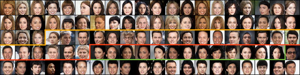
A variety of socio-technical factors contribute to the discriminatory nature of ML systems (Barocas et al. 2018). A major factor is the existence of biases in the training data itself (Torralba et al. 2011; Tommasi et al. 2017). Since data is the fuel of ML, any existing bias in the dataset can be propagated to the learned model (Barocas & Selbst 2016). This is a particularly pressing concern for generative models which can easily amplify the bias by generating more of the biased data at test time. Further, learning a generative model is fundamentally an unsupervised learning problem and hence, the bias factors of interest are typically latent. For example, while learning a generative model of human faces, we often do not have access to attributes such as gender, race, and age. Any existing bias in the dataset with respect to these attributes are easily picked by deep generative models. See Figure 1 for an illustration.

Refer to caption — Figure 1: Samples from a baseline BigGAN that reflect the gender bias underlying the true data distribution in CelebA. All faces above the orange line (67%) are classified as female, while the rest are labeled as male (33%).

In this work, we present a weakly-supervised approach to learning fair generative models in the presence of dataset bias. Our source of weak supervision is motivated by the observation that obtaining multiple unlabelled (biased) datasets is relatively cheap for many domains in the big data era. Among these data sources, we may wish to generate samples that are close in distribution to a particular target (reference) dataset.¹¹ 1 We note that while there may not be concept of a dataset devoid of bias, carefully designed representative data collection practices may be more accurately reflected in some data sources (Gebru et al. 2018) and can be considered as reference datasets. As a concrete example of such a reference, organizations such as the World Bank and biotech firms (23&me 2016; Hong 2016) typically follow several good practices to ensure representativeness in the datasets that they collect, though such methods are unscalable to large sizes. We note that neither of our datasets need to be labeled w.r.t. the latent bias attributes and the size of the reference dataset can be much smaller than the biased dataset. Hence, the level of supervision we require is weak.

Using a reference dataset to augment a biased dataset, our goal is to learn a generative model that best approximates the desired, reference data distribution. Simply using the reference dataset alone for learning is an option, but this may not suffice since this dataset can be too small to learn an expressive model that accurately captures the underlying reference data distribution. Our approach to learning a fair generative model that is robust to biases in the larger training set is based on importance reweighting. In particular, we learn a generative model which reweighs the data points in the biased dataset based on the ratio of densities assigned by the biased data distribution as compared to the reference data distribution. Since we do not have access to explicit densities assigned by either of the two distributions, we estimate the weights by using a probabilistic classifier (Sugiyama et al. 2012; Mohamed & Lakshminarayanan 2016).

We test our weakly-supervised approach on learning generative adversarial networks on the CelebA dataset (Ziwei Liu & Tang 2015). The dataset consists of attributes such as gender and hair color, which we use for designing biased and reference data splits and subsequent evaluation. We empirically demonstrate how the reweighting approach can offset dataset bias on a wide range of settings. In particular, we obtain improvements of up to 36.6% (49.3% for bias=0.9 and 23.9% for bias=0.8) for single-attribute dataset bias and 32.5% for multi-attribute dataset bias on average over baselines in reducing the bias with respect to the latent factors for comparable sample quality.

2 Problem Setup

2.1 Background

We assume there exists a true (unknown) data distribution $p_{\rm{data}}:{\mathcal{X}}\to{\mathbb{R}}_{\geq 0}$ over a set of $d$ observed variables ${\mathbf{x}}\in{\mathbb{R}}^{d}$ . In generative modeling, our goal is to learn the parameters $\theta\in\Theta$ of a distribution $p_{\theta}:{\mathcal{X}}\to{\mathbb{R}}_{\geq 0}$ over the observed variables ${\mathbf{x}}$ , such that the model distribution $p_{\theta}$ is close to $p_{\rm{data}}$ . Depending on the choice of learning algorithm, different approaches have been previously considered. Broadly, these include adversarial training e.g., GANs (Goodfellow et al. 2014) and maximum likelihood estimation (MLE) e.g., variational autoencoders (VAE) (Kingma & Welling 2013; Rezende et al. 2014) and normalizing flows (Dinh et al. 2014) or hybrids (Grover et al. 2018). Our bias mitigation framework is agnostic to the above training approaches.

For generality, we consider expectation-based learning objectives, where $\ell(\cdot)$ is a per-example loss that depends on both examples ${\mathbf{x}}$ drawn from a dataset ${\mathcal{D}}$ and the model parameters $\theta$ :

\displaystyle{\mathbb{E}}_{{\mathbf{x}}\sim p_{\rm{data}}}[\ell({\mathbf{x}},\theta)]\approx\frac{1}{T}\sum_{i=1}^{T}\ell({\mathbf{x}}_{i},\theta):={\mathcal{L}}(\theta;{\mathcal{D}})

(1)

The above expression encompasses a broad class of MLE and adversarial objectives. For example, if $\ell(\cdot)$ denotes the negative log-likelihood assigned to the point ${\mathbf{x}}$ as per $p_{\theta}$ , then we recover the MLE training objective.

2.2 Dataset Bias

The standard assumption for learning a generative model is that we have access to a sufficiently large dataset ${\mathcal{D}_{\mathrm{ref}}}$ of training examples, where each ${\mathbf{x}}\in{\mathcal{D}_{\mathrm{ref}}}$ is assumed to be sampled independently from a reference distribution $p_{\rm{data}}=p_{\rm{ref}}$ . In practice however, collecting large datasets that are i.i.d. w.r.t. $p_{\rm{ref}}$ is difficult due to a variety of socio-technical factors. The sample complexity for learning high dimensional distributions can even be doubly-exponential in the dimensions in many cases (Arora et al. 2018), surpassing the size of the largest available datasets.

We can partially offset this difficulty by considering data from alternate sources related to the target distribution, e.g., images scraped from the Internet. However, these additional datapoints are not expected to be i.i.d. w.r.t. $p_{\rm{ref}}$ .

We characterize this phenomena as dataset bias, where we assume the availability of a dataset ${\mathcal{D}_{\mathrm{bias}}}$ , such that the examples ${\mathbf{x}}\in{\mathcal{D}_{\mathrm{bias}}}$ are sampled independently from a biased (unknown) distribution $p_{\rm{bias}}$ that is different from $p_{\rm{ref}}$ , but shares the same support.

2.3 Evaluation

Evaluating generative models and fairness in machine learning are both open areas of research. Our work is at the intersection of these two fields and we propose the following metrics for measuring bias mitigation for data generation.

Sample Quality:

We employ sample quality metrics e.g., Frechet Inception Distance (FID) (Heusel et al. 2017), Kernel Inception Distance (KID) (Li et al. 2017), etc. These metrics match empirical expectations w.r.t. a reference data distribution $p$ and a model distribution $p_{\theta}$ in a predefined feature space e.g., the prefinal layer of activations of Inception Network (Szegedy et al. 2016). A lower score indicates that the learned model can better approximate $p_{\rm{data}}$ . For the fairness context in particular, we are interested in measuring the discrepancy w.r.t. $p_{\rm{ref}}$ even if the model has been trained to use both ${\mathcal{D}_{\mathrm{ref}}}$ and ${\mathcal{D}_{\mathrm{bias}}}$ . We refer the reader to Supplement B.2 for more details on evaluation with FID.

Fairness:

Alternatively, we can evaluate bias of generative models specifically in the context of some sensitive latent variables, say ${\mathbf{u}}\in{\mathbb{R}}^{k}$ . For example, ${\mathbf{u}}$ may correspond to the age and gender of an individual depicted via an image ${\mathbf{x}}$ . We emphasize that such attributes are unknown during training, and used only for evaluation at test time.

If we have access to a highly accurate predictor $p({\mathbf{u}}|{\mathbf{x}})$ for the distribution of the sensitive attributes ${\mathbf{u}}$ conditioned on the observed ${\mathbf{x}}$ , we can evaluate the extent of bias mitigation via the discrepancies in the expected marginal likelihoods of ${\mathbf{u}}$ as per $p_{\rm{ref}}$ and $p_{\theta}$ .

Formally, we define the fairness discrepancy $f$ for a generative model $p_{\theta}$ w.r.t. $p_{\rm{ref}}$ and sensitive attributes ${\mathbf{u}}$ :

\displaystyle f(p_{\rm{ref}},p_{\theta})=|{\mathbb{E}}_{p_{\rm{ref}}}[p({\mathbf{u}}|{\mathbf{x}})]-{\mathbb{E}}_{p_{\theta}}[p({\mathbf{u}}|{\mathbf{x}})]|_{2}.

(2)

In practice, the expectations in Eq. equation 2 can be computed via Monte Carlo averaging. Again the lower is the discrepancy in the above two expectations, the better is the learned model’s ability to mitigate dataset bias w.r.t. the sensitive attributes ${\mathbf{u}}$ . We refer the reader to Supplement E for more details on the fairness discrepancy metric.

3 Bias Mitigation

We assume a learning setting where we are given access to a data source ${\mathcal{D}_{\mathrm{bias}}}$ in addition to a dataset of training examples ${\mathcal{D}_{\mathrm{ref}}}$ . Our goal is to capitalize on both data sources ${\mathcal{D}_{\mathrm{bias}}}$ and ${\mathcal{D}_{\mathrm{ref}}}$ for learning a model $p_{\theta}$ that best approximates the target distribution $p_{\rm{ref}}$ .

3.1 Baselines

We begin by discussing two baseline approaches at the extreme ends of the spectrum. First, one could completely ignore ${\mathcal{D}_{\mathrm{bias}}}$ and consider learning $p_{\theta}$ based on ${\mathcal{D}_{\mathrm{ref}}}$ alone. Since we only consider proper losses w.r.t. $p_{\rm{ref}}$ , global optimization of the objective in Eq. equation 1 in a well-specified model family will recover the true data distribution as $|{\mathcal{D}_{\mathrm{ref}}}|\to\infty$ . However, since ${\mathcal{D}_{\mathrm{ref}}}$ is finite in practice, this is likely to give poor sample quality even though the fairness discrepancy would be low.

On the other extreme, we can consider learning $p_{\theta}$ based on the full dataset consisting of both ${\mathcal{D}_{\mathrm{ref}}}$ and ${\mathcal{D}_{\mathrm{bias}}}$ . This procedure will be data efficient and could lead to high sample quality, but it comes at the cost of fairness since the learned distribution will be heavily biased w.r.t. $p_{\rm{ref}}$ .

3.2 Solution 1: Conditional Modeling

Our first proposal is to learn a generative model conditioned on the identity of the dataset used during training. Formally, we learn a generative model $p_{\theta}({\mathbf{x}}|y)$ where $y\in\{0,1\}$ is a binary random variable indicating whether the model distribution was learned to approximate the data distribution corresponding to ${\mathcal{D}_{\mathrm{ref}}}$ (i.e., $p_{\rm{ref}}$ ) or ${\mathcal{D}_{\mathrm{bias}}}$ (i.e., $p_{\rm{bias}}$ ). By sharing model parameters $\theta$ across the two values of $y$ , we hope to leverage both data sources. At test time, conditioning on $y$ for ${\mathcal{D}_{\mathrm{ref}}}$ should result in fair generations.

As we demonstrate in Section 4 however, this simple approach does not achieve the intended effect in practice. The likely cause is that the conditioning information is too weak for the model to infer the bias factors and effectively distinguish between the two distributions. Next, we present an alternate two-phased approach based on density ratio estimation which effectively overcomes the dataset bias in a data-efficient manner.

3.3 Solution 2: Importance Reweighting

Recall a trivial baseline in Section 3.1 which learns a generative model on the union of ${\mathcal{D}_{\mathrm{bias}}}$ and ${\mathcal{D}_{\mathrm{ref}}}$ . This method is problematic because it assigns equal weight to the loss contributions from each individual datapoint in our dataset in Eq. equation 1, regardless of whether the datapoint comes from ${\mathcal{D}_{\mathrm{bias}}}$ or ${\mathcal{D}_{\mathrm{ref}}}$ . For example, in situations where the dataset bias causes a minority group to be underrepresented, this objective will encourage the model to focus on the majority group such that the overall value of the loss is minimized on average with respect to a biased empirical distribution i.e., a weighted mixture of $p_{\rm{bias}}$ and $p_{\rm{ref}}$ with weights proportional to $|{\mathcal{D}_{\mathrm{bias}}}|$ and $|{\mathcal{D}_{\mathrm{ref}}}|$ .

Our key idea is to reweight the datapoints from ${\mathcal{D}_{\mathrm{bias}}}$ during training such that the model learns to downweight over-represented data points from ${\mathcal{D}_{\mathrm{bias}}}$ while simultaneously upweighting the under-represented points from ${\mathcal{D}_{\mathrm{ref}}}$ . The challenge in the unsupervised context is that we do not have direct supervision on which points are over- or under-represented and by how much. To resolve this issue, we consider importance sampling (Horvitz & Thompson 1952). Whenever we are given data from two distributions, w.l.o.g. say $p$ and $q$ , and wish to evaluate a sample average w.r.t. $p$ given samples from $q$ , we can do so by reweighting the samples from $p$ by the ratio of densities assigned to the sampled points by $p$ and $q$ . In our setting, the distributions of interest are $p_{\rm{bias}}$ and $p_{\rm{ref}}$ respectively. Hence, an importance weighted objective for learning from ${\mathcal{D}_{\mathrm{bias}}}$ is:

	$\displaystyle{\mathbb{E}}_{{\mathbf{x}}\sim p_{\rm{ref}}}[\ell({\mathbf{x}},\theta)]$	$\displaystyle={\mathbb{E}}_{{\mathbf{x}}\sim p_{\rm{bias}}}\left[\frac{p_{\rm{ref}}({\mathbf{x}})}{p_{\rm{bias}}({\mathbf{x}})}\ell({\mathbf{x}},\theta)\right]$		(3)
		$\displaystyle\approx\frac{1}{T}\sum_{i=1}^{T}w({\mathbf{x}}_{i})\ell({\mathbf{x}}_{i},\theta):={\mathcal{L}}(\theta,{\mathcal{D}_{\mathrm{bias}}})$		(4)

where $w({\mathbf{x}}_{i}):=\frac{p_{\rm{ref}}({\mathbf{x}})}{p_{\rm{bias}}({\mathbf{x}})}$ is defined to be the importance weight for ${\mathbf{x}}_{i}\sim p_{\rm{bias}}$ .

Estimating density ratios via binary classification.

To estimate the importance weights, we use a binary classifier as described below (Sugiyama et al. 2012).

Consider a binary classification problem with classes $Y\in\{0,1\}$ with training data generated as follows. First, we fix a prior probability for $p(Y=1)$ . Then, we repeatedly sample $y\sim p(Y)$ . If $y=1$ , we independently sample a datapoint ${\mathbf{x}}\sim p_{\rm{ref}}$ , else we sample ${\mathbf{x}}\sim p_{\rm{bias}}$ . Then, as shown in Friedman et al. 2001, the ratio of densities $p_{\rm{ref}}$ and $p_{\rm{bias}}$ assigned to an arbitrary point ${\mathbf{x}}$ can be recovered via a Bayes optimal (probabilistic) classifier $c^{\ast}:{\mathcal{X}}\to[0,1]$ :

\displaystyle w({\mathbf{x}})=\frac{p_{\rm{ref}}({\mathbf{x}})}{p_{\rm{bias}}({\mathbf{x}})}=\gamma\frac{c^{\ast}(Y=1|x)}{1-c^{\ast}(Y=1|x)}

(5)

where $c(Y=1|x)$ is the probability assigned by the classifier to the point ${\mathbf{x}}$ belonging to class $Y=1$ . Here, $\gamma=\frac{p(Y=0)}{p(Y=1)}$ is the ratio of marginals of the labels for two classes.

In practice, we do not have direct access to either $p_{\rm{bias}}$ or $p_{\rm{ref}}$ and hence, our training data consists of points sampled from the empirical data distributions defined uniformly over ${\mathcal{D}_{\mathrm{ref}}}$ and ${\mathcal{D}_{\mathrm{bias}}}$ . Further, we may not be able to learn a Bayes optimal classifier and denote the importance weights estimated by the learned classifier $c$ for a point ${\mathbf{x}}$ as $\hat{w}({\mathbf{x}})$ .

Algorithm 1 Learning Fair Generative Models

Input: ${\mathcal{D}_{\mathrm{bias}}},{\mathcal{D}_{\mathrm{ref}}}$ , Classifier and Generative Model Architectures & Hyperparameters
Output: Generative Model Parameters $\theta$

\triangleright

Phase 1: Estimate importance weights

2: Learn binary classifier

c

for distinguishing

({\mathcal{D}_{\mathrm{bias}}},Y=0)

vs.

({\mathcal{D}_{\mathrm{ref}}},Y=1)

3: Estimate importance weight

\hat{w}({\mathbf{x}})\leftarrow\frac{c(Y=1|{\mathbf{x}})}{c(Y=0|{\mathbf{x}})}

for all

{\mathbf{x}}\in{\mathcal{D}_{\mathrm{bias}}}

(using Eq. 5)

4: Set importance weight

\hat{w}({\mathbf{x}})\leftarrow 1

for all

{\mathbf{x}}\in{\mathcal{D}_{\mathrm{ref}}}

\triangleright

Phase 2: Minibatch gradient descent on

\theta

based on weighted loss

6: Initialize model parameters

\theta

at random

7: Set full dataset

{\mathcal{D}}\leftarrow{\mathcal{D}_{\mathrm{bias}}}\cup{\mathcal{D}_{\mathrm{ref}}}

8: while training do

9: Sample a batch of points

B

from

{\mathcal{D}}

at random

10: Set loss

{\mathcal{L}}(\theta;{\mathcal{D}})\leftarrow\frac{1}{|B|}\sum_{{\mathbf{x}}_{i}\in B}\hat{w}({\mathbf{x}}_{i})\ell({\mathbf{x}}_{i},\theta)

11: Estimate gradients

\nabla_{\theta}{\mathcal{L}}(\theta;{\mathcal{D}})

and update parameters

\theta

based on optimizer update rule

12: end while

13: return

\theta

Our overall procedure is summarized in Algorithm 1. We use deep neural networks for parameterizing the binary classifier and the generative model. Given a biased and reference dataset along with the network architectures and other standard hyperparameters (e.g., learning rate, optimizer etc.), we first learn a probabilistic binary classifier (Line 2). The learned classifier can provide importance weights for the datapoints from ${\mathcal{D}_{\mathrm{bias}}}$ via estimates of the density ratios (Line 3). For the datapoints from ${\mathcal{D}_{\mathrm{ref}}}$ , we do not need to perform any reweighting and set the importance weights to 1 (Line 4). Using the combined dataset ${\mathcal{D}_{\mathrm{bias}}}\cup{\mathcal{D}_{\mathrm{ref}}}$ , we then learn the generative model $p_{\theta}$ where the minibatch loss for every gradient update weights the contributions from each datapoint (Lines 6-12).

For a practical implementation, it is best to account for some diagnostics and best practices while executing Algorithm 1. For density ratio estimation, we test that the classifier is calibrated on a held out set. This is a necessary (but insufficient) check for the estimated density ratios to be meaningful. If the classifier is miscalibrated, we can apply standard recalibration techniques such as Platt scaling before estimating the importance weights. Furthermore, while optimizing the model using a weighted objective, there can be an increased variance across the loss contributions from each example in a minibatch due to importance weighting. We did not observe this in our experiments, but techniques such as normalization of weights within a batch can potentially help control the unintended variance introduced within a batch (Sugiyama et al. 2012).

Theoretical Analysis. The performance of Algorithm 1 critically depends on the quality of estimated density ratios, which in turn is dictated by the training of the binary classifier. We define the expected negative cross-entropy (NCE) objective for a classifier $c$ as:

	$\displaystyle NCE(c)$	$\displaystyle:=\frac{1}{\gamma+1}{\mathbb{E}}_{p_{\rm{ref}}({\mathbf{x}})}[\log c(Y=1\|{\mathbf{x}})]$
		$\displaystyle+\frac{\gamma}{\gamma+1}{\mathbb{E}}_{p_{\rm{bias}}({\mathbf{x}})}[\log c(Y=0\|{\mathbf{x}})].$		(6)

In the following result, we characterize the NCE loss for the Bayes optimal classifier.

Theorem 1.

Let $\mathcal{Z}$ denote a set of unobserved bias variables. Suppose there exist two joint distributions $p_{\rm{bias}}({\mathbf{x}},{\mathbf{z}})$ and $p_{\rm{ref}}({\mathbf{x}},{\mathbf{z}})$ over ${\mathbf{x}}\in\mathcal{X}$ and ${\mathbf{z}}\in\mathcal{Z}$ . Let $p_{\rm{bias}}({\mathbf{x}})$ and $p_{\rm{bias}}({\mathbf{z}})$ denote the marginals over ${\mathbf{x}}$ and ${\mathbf{z}}$ for the joint $p_{\rm{bias}}({\mathbf{x}},{\mathbf{z}})$ and similar notation for the joint $p_{\rm{ref}}({\mathbf{x}},{\mathbf{z}})$ :

\displaystyle p_{\rm{bias}}({\mathbf{x}}|{\mathbf{z}}=k)

\displaystyle=p_{\rm{ref}}({\mathbf{x}}|{\mathbf{z}}=k)\;\;\forall k

(7)

and $p_{\rm{bias}}({\mathbf{x}}|{\mathbf{z}}=k)$ , $p_{\rm{bias}}({\mathbf{x}}|{\mathbf{z}}=k^{\prime})$ have disjoint supports for $k\neq k^{\prime}$ . Then, the negative cross-entropy of the Bayes optimal classifier $c^{\ast}$ is given as:

	$\displaystyle NCE(c^{\ast})$	$\displaystyle=\frac{1}{\gamma+1}{\mathbb{E}}_{p_{\rm{ref}}({\mathbf{z}})}\left[\log\frac{1}{\gamma b({\mathbf{z}})+1}\right]$
		$\displaystyle+\frac{\gamma}{\gamma+1}{\mathbb{E}}_{p_{\rm{bias}}({\mathbf{z}})}\left[\log\frac{\gamma b({\mathbf{z}})}{\gamma b({\mathbf{z}})+1}\right].$		(8)

where $b({\mathbf{z}})=p_{\rm{bias}}({\mathbf{z}})/p_{\rm{ref}}({\mathbf{z}})$ .

Proof.

See Supplement A. ∎

For example, as we shall see in our experiments in the following section, the inputs ${\mathbf{x}}$ can correspond to face images, whereas the unobserved ${\mathbf{z}}$ represents sensitive bias factors for a subgroup such as gender or ethnicity. The proportion of examples ${\mathbf{x}}$ belonging a subgroup can differ across the biased and reference datasets with the relative proportions given by $b(\mathbf{z})$ . Note that the above result only requires knowing these relative proportions and not the true ${\mathbf{z}}$ for each ${\mathbf{x}}$ . The practical implication is that under the assumptions of Theorem 1, we can check the quality of density ratios estimated by an arbitrary learned classifier $c$ by comparing its empirical NCE with the theoretical NCE of the Bayes optimal classifier in Eq. 1 (see Section 4.1).

4 Empirical Evaluation

In this section, we are interested in investigating two broad questions empirically:

1.

How well can we estimate density ratios for the proposed weak supervision setting?
2.

How effective is the reweighting technique for learning fair generative models on the fairness discrepancy metric proposed in Section 2.3?

We further demonstrate the usefulness of our generated data in downstream applications such as data augmentation for learning a fair classifier in Supplement F.3.

Dataset. We consider the CelebA (Ziwei Liu & Tang 2015) dataset, which is commonly used for benchmarking deep generative models and comprises of images of faces with 40 labeled binary attributes. We use this attribute information to construct 3 different settings for partitioning the full dataset into ${\mathcal{D}_{\mathrm{bias}}}$ and ${\mathcal{D}_{\mathrm{ref}}}$ .

•

Setting 1 (single, bias=0.9): We set ${\mathbf{z}}$ to be a single bias variable corresponding to “gender” with values 0 (female) and 1 (male) and $b({\mathbf{z}}=0)=0.9$ .

Specifically, this means that ${\mathcal{D}_{\mathrm{ref}}}$ contains the same fraction of male and female images whereas ${\mathcal{D}_{\mathrm{bias}}}$ contains 0.9 fraction of females and rest as males.
•

Setting 2 (single, bias=0.8): We use same bias variable (gender) as Setting 1 with $b({\mathbf{z}}=0)=0.8$ .
•

Setting 3 (multi): We set ${\mathbf{z}}$ as two bias variables corresponding to “gender” and “black hair”. In total, we have 4 subgroups: females without black hair (00), females with black hair (01), males without black hair (10), and males with black hair (11). We set $b({\mathbf{z}}=00)=0.437,b({\mathbf{z}}=01)=0.063,b({\mathbf{z}}=10)=0.415,b({\mathbf{z}}=11)=0.085$ .

We emphasize that the attribute information is used only for designing controlled biased and reference datasets and faithful evaluation. Our algorithm does not explicitly require such labeled information. Additional information on constructing the dataset splits can be found in Supplement B.1.

Models. We train two classifiers for our experiments: (1) the attribute (e.g. gender) classifier which we use to assess the level of bias present in our final samples; and (2) the density ratio classifier. For both models, we use a variant of ResNet18 (He et al. 2016) on the standard train and validation splits of CelebA. For the generative model, we used a BigGAN (Brock et al. 2018) trained to minimize the hinge loss (Lim & Ye 2017; Tran et al. 2017) objective. Additional details regarding the architectural design and hyperparameters in Supplement C.

4.1 Density Ratio Estimation via Classifier

For each of the three experiments settings, we can evaluate the quality of the estimated density ratios by comparing empirical estimates of the cross-entropy loss of the density ratio classifier with the cross-entropy loss of the Bayes optimal classifier derived in Eq. 1. We show the results in Table 1 for perc=1.0 where we find that the two losses are very close, suggesting that we obtain high-quality density ratio estimates that we can use for subsequently training fair generative models. In Supplement D, we show a more fine-grained analysis of the 0-1 accuracies and calibration of the learned models.

Model	Bayes optimal	Empirical
single, bias=0.9	0.591	0.605
single, bias=0.8	0.642	0.650
multi	0.619	0.654

Table 1: Comparison between the cross-entropy loss of the Bayes classifier and learned density ratio classifier.

In Figure 2, we show the distribution of our importance weights for the various latent subgroups. We find that across all the considered settings, the underrepresented subgroups (e.g., males in Figure 2(a), 2(b), females with black hair in 2(c)) are upweighted on average (mean density ratio estimate $>$ 1), while the overrepresented subgroups are downweighted on average (mean density ratio estimate $<$ 1). Also, as expected, the density ratio estimates are closer to 1 when the bias is low (see Figure 2(a) v.s. 2(b)).

4.2 Fair Data Generation

We compare our importance weighted approach against three baselines: (1) equi-weight: a BigGAN trained on the full dataset ${\mathcal{D}_{\mathrm{ref}}}\cup{\mathcal{D}_{\mathrm{bias}}}$ that weighs every point equally; (2) reference-only: a BigGAN trained on the reference dataset ${\mathcal{D}_{\mathrm{ref}}}$ ; and (3) conditional: a conditional BigGAN where the conditioning label indicates whether a data point ${\mathbf{x}}$ is from ${\mathcal{D}_{\mathrm{ref}}}(y=1)$ or ${\mathcal{D}_{\mathrm{bias}}}(y=0)$ . In all our experiments, the reference-only variant which only uses the reference dataset ${\mathcal{D}_{\mathrm{ref}}}$ for learning however failed to give any recognizable samples. For a clean presentation of the results due to other methods, we hence ignore this baseline in the results below and defer the reader to the supplementary material for further results.

We also vary the size of the balanced dataset ${\mathcal{D}_{\mathrm{ref}}}$ relative to the unbalanced dataset size $|{\mathcal{D}_{\mathrm{bias}}}|$ : perc = {0.1, 0.25, 0.5, 1.0}. Here, perc = 0.1 denotes $|{\mathcal{D}_{\mathrm{ref}}}|$ = 10% of $|{\mathcal{D}_{\mathrm{bias}}}|$ and perc = 1.0 denotes $|{\mathcal{D}_{\mathrm{ref}}}|=|{\mathcal{D}_{\mathrm{bias}}}|$ .

4.2.1 Single Attribute Splits

We train our attribute (gender) classifier for evaluation on the entire CelebA training set, and achieve a level of 98% accuracy on the held-out set. For each experimental setting, we evaluate bias mitigation based on the fairness discrepancy metric (Eq. 2) and also report sample quality based on FID (Heusel et al. 2017).

For the bias = 0.9 split, we show the samples generated via imp-weight in Figure 3a and the resulting fairness discrepancies in Figure 3b. Our framework generates samples that are slightly lower quality than equi-weight baseline samples shown in Figure 1, but is able to produce almost identical proportion of samples across the two genders. Similar observations hold for bias = 0.8, as shown in Figure 8 in the supplement. We refer the reader to Supplement F.4 for corresponding results and analysis, as well as for additional results on the Shapes3D dataset (Burgess & Kim 2018).

4.2.2 Multi-Attribute Split

We conduct a similar experiment with a multi-attribute split based on gender and the presence of black hair. The attribute classifier for the purpose of evaluation is now trained with a 4-way classification task instead of 2, and achieves an accuracy of roughly 88% on the test set.

Our model produces samples as shown in Figure 4a with the discrepancy metrics shown in Figures 4b, c respectively. Even in this challenging setup involving two latent bias factors, we find that the importance weighted approach again outperforms the baselines in almost all cases in mitigating bias in the generated data while admitting only a slight deterioration in image quality overall.

5 Related Work

Fairness & generative modeling. There is a rich body of work in fair ML, which focus on different notions of fairness (e.g. demographic parity, equality of odds and opportunity) and study methods by which models can perform tasks such as classification in a non-discriminatory way (Barocas et al. 2018; Dwork et al. 2012; Heidari et al. 2018; du Pin Calmon et al. 2018). Our focus is in the context of fair generative modeling. The vast majority of related work in this area is centered around fair and/or privacy preserving representation learning, which exploit tools from adversarial learning and information theory among others (Zemel et al. 2013; Edwards & Storkey 2015; Louizos et al. 2015; Beutel et al. 2017; Song et al. 2018; Adel et al. 2019). A unifying principle among these methods is such that a discriminator is trained to perform poorly in predicting an outcome based on a protected attribute. Ryu et al. 2017 considers transfer learning of race and gender identities as a form of weak supervision for predicting other attributes on datasets of faces. While the end goal for the above works is classification, our focus is on data generation in the presence of dataset bias and we do not require explicit supervision for the protected attributes.

The most relevant prior works in data generation are FairGAN (Xu et al. 2018) and FairnessGAN (Sattigeri et al. 2019). The goal of both methods is to generate fair datapoints and their labels as a preprocessing technique. This allows for learning a useful downstream classifier and obscures information about protected attributes. Again, these works are not directly comparable to ours as we do not assume explicit supervision regarding the protected attributes during training, and our goal is fair generation given unlabelled biased datasets where the bias factors are latent. Another relevant work is DB-VAE (Amini et al. 2019), which utilizes a VAE to learn the latent structure of sensitive attributes, and in turn employs importance weighting based on this structure to mitigate bias in downstream classifiers. Contrary to our work, these importance weights are used to directly sample (rare) data points with higher frequencies with the goal of training a classifier (e.g. as in a facial detection system), as opposed to fair generation.

Importance reweighting. Reweighting datapoints is a common algorithmic technique for problems such as dataset bias and class imbalance (Byrd & Lipton 2018). It has often been used in the context of fair classification (Calders et al. 2009), for example, (Kamiran & Calders 2012) details reweighting as a way to remove discrimination without relabeling instances. For reinforcement learning, Doroudi et al. 2017 used an importance sampling approach for selecting fair policies. There is also a body of work on fair clustering (Chierichetti et al. 2017; Backurs et al. 2019; Bera et al. 2019; Schmidt et al. 2018) which ensure that the clustering assignments are balanced with respect to some sensitive attribute.

Density ratio estimation using classifiers. The use of classifiers for estimating density ratios has a rich history of prior works across ML (Sugiyama et al. 2012). For deep generative modeling, density ratios estimated by classifiers have been used for expanding the class of various learning objectives (Nowozin et al. 2016; Mohamed & Lakshminarayanan 2016; Grover & Ermon 2018), evaluation metrics based on two-sample tests (Gretton et al. 2007; Bowman et al. 2015; Lopez-Paz & Oquab 2016; Danihelka et al. 2017; Rosca et al. 2017; Im et al. 2018; Gulrajani et al. 2018), or improved Monte Carlo inference via these models (Grover et al. 2019; Azadi et al. 2018; Turner et al. 2018; Tao et al. 2018). Grover et al. 2019 use importance reweighting for mitigating model bias between $p_{\rm{data}}$ and $p_{\theta}$ .

Closest related is the proposal of Diesendruck et al. 2018 to use importance reweighting for learning generative models where training and test distributions differ, but explicit importance weights are provided for at least a subset of the training examples. We consider a more realistic, weakly-supervised setting where we estimate the importance weights using a small reference dataset. Finally, another related line of work in domain translation via generation considers learning via multiple datasets (Zhu et al. 2017; Choi & Jang 2018; Grover et al. 2020) and it would be interesting to consider issues due to dataset bias in those settings in future work.

6 Discussion

Our work presents an initial foray into the field of fair image generation with weak supervision, and we stress the need for caution in using our techniques and interpreting the empirical findings. For scaling our evaluation, we proposed metrics that relied on a pretrained attribute classifier for inferring the bias in the generated data samples. The classifiers we considered are highly accurate on all subgroups, but can have blind spots especially when evaluated on generated data. For future work, we would like to investigate conducting human evaluations to mitigate such issues during evaluation (Grgic-Hlaca et al. 2018).

As another case in point, our work calls for rethinking sample quality metrics for generative models in the presence of dataset bias (Mitchell et al. 2019). On one hand, our approach increases the diversity of generated samples in the sense that the different subgroups are more balanced; at the same time, however, variation across other image features decreases because the newly generated underrepresented samples are learned from a smaller dataset of underrepresented subgroups. Moreover, standard metrics such as FID even when evaluated with respect to a reference dataset, could exhibit a relative preference for models trained on larger datasets with little or no bias correction to avoid even slight compromises on perceptual sample quality.

More broadly, this work is yet another reminder that we must be mindful of the decisions made at each stage in the development and deployment of ML systems (Abebe et al. 2020). Factors such as the dataset used for training (Gebru et al. 2018; Sheng et al. 2019; Jo & Gebru 2020) or algorithmic decisions such as the loss function or evaluation metric (Hardt et al. 2016; Buolamwini & Gebru 2018; Kim et al. 2018; Liu et al. 2018; Hashimoto et al. 2018), among others, may have undesirable consequences. Becoming more aware of these downstream impacts will help to mitigate the potentially discriminatory nature of our present-day systems (Kaeser-Chen et al. 2020).

7 Conclusion

We considered the task of fair data generation given access to a (potentially small) reference dataset and a large biased dataset. For data-efficient learning, we proposed an importance weighted objective that corrects bias by reweighting the biased datapoints. These weights are estimated by a binary classifier. Empirically, we showed that our technique outperforms baselines by up to 34.6% on average in reducing dataset bias on CelebA without incurring a significant reduction in sample quality. We provide reference implementations in PyTorch (Paszke et al. 2017), and the codebase for this work is open-sourced at https://github.com/ermongroup/fairgen.

In the future, it would be interesting to explore whether even weaker forms of supervision would be possible for this task, e.g., when the biased dataset has a somewhat disjoint but related support from the small, reference dataset – this would be highly reflective of the diverse data sources used for training many current and upcoming large-scale ML systems (Ratner et al. 2017).

Acknowledgements

We are thankful to Hima Lakkaraju, Daniel Levy, Mike Wu, Chris Cundy, and Jiaming Song for insightful discussions and feedback. KC is supported by the NSF GRFP, Qualcomm Innovation Fellowship, and Stanford Graduate Fellowship, and AG is supported by the MSR Ph.D. fellowship, Stanford Data Science scholarship, and Lieberman fellowship. This research was funded by NSF (#1651565, #1522054, #1733686), ONR (N00014-19-1-2145), AFOSR (FA9550-19-1-0024), and Amazon AWS.

References

23&me (2016) 23&me. The real issue: Diversity in genetics research. Retrieved from https://blog.23andme.com/ancestry/the-real-issue-diversity-in-genetics-research/, 2016.
Abebe et al. (2020) Abebe, R., Barocas, S., Kleinberg, J., Levy, K., Raghavan, M., and Robinson, D. G. Roles for computing in social change. In Proceedings of the 2020 Conference on Fairness, Accountability, and Transparency, pp. 252–260, 2020.
Adel et al. (2019) Adel, T., Valera, I., Ghahramani, Z., and Weller, A. One-network adversarial fairness. 2019.
Amini et al. (2019) Amini, A., Soleimany, A. P., Schwarting, W., Bhatia, S. N., and Rus, D. Uncovering and mitigating algorithmic bias through learned latent structure. In Proceedings of the 2019 AAAI/ACM Conference on AI, Ethics, and Society, pp. 289–295, 2019.
Arora et al. (2018) Arora, S., Risteski, A., and Zhang, Y. Do gans learn the distribution? some theory and empirics. In International Conference on Learning Representations, 2018.
Azadi et al. (2018) Azadi, S., Olsson, C., Darrell, T., Goodfellow, I., and Odena, A. Discriminator rejection sampling. arXiv preprint arXiv:1810.06758, 2018.
Backurs et al. (2019) Backurs, A., Indyk, P., Onak, K., Schieber, B., Vakilian, A., and Wagner, T. Scalable fair clustering. arXiv preprint arXiv:1902.03519, 2019.
Barocas & Selbst (2016) Barocas, S. and Selbst, A. D. Big data’s disparate impact. Calif. L. Rev., 104:671, 2016.
Barocas et al. (2018) Barocas, S., Hardt, M., and Narayanan, A. Fairness and Machine Learning. fairmlbook.org, 2018. http://www.fairmlbook.org.
Bera et al. (2019) Bera, S. K., Chakrabarty, D., and Negahbani, M. Fair algorithms for clustering. arXiv preprint arXiv:1901.02393, 2019.
Beutel et al. (2017) Beutel, A., Chen, J., Zhao, Z., and Chi, E. H. Data decisions and theoretical implications when adversarially learning fair representations. arXiv preprint arXiv:1707.00075, 2017.
Bowman et al. (2015) Bowman, S. R., Vilnis, L., Vinyals, O., Dai, A. M., Jozefowicz, R., and Bengio, S. Generating sentences from a continuous space. arXiv preprint arXiv:1511.06349, 2015.
Brock et al. (2018) Brock, A., Donahue, J., and Simonyan, K. Large scale gan training for high fidelity natural image synthesis. arXiv preprint arXiv:1809.11096, 2018.
Brown et al. (2020) Brown, T. B., Mann, B., Ryder, N., Subbiah, M., Kaplan, J., Dhariwal, P., Neelakantan, A., Shyam, P., Sastry, G., Askell, A., Agarwal, S., Herbert-Voss, A., Krueger, G., Henighan, T., Child, R., Ramesh, A., Ziegler, D. M., Wu, J., Winter, C., Hesse, C., Chen, M., Sigler, E., Litwin, M., Gray, S., Chess, B., Clark, J., Berner, C., McCandlish, S., Radford, A., Sutskever, I., and Amodei, D. Language models are few-shot learners. 2020.
Buolamwini & Gebru (2018) Buolamwini, J. and Gebru, T. Gender shades: Intersectional accuracy disparities in commercial gender classification. In Conference on fairness, accountability and transparency, pp. 77–91, 2018.
Burgess & Kim (2018) Burgess, C. and Kim, H. 3d shapes dataset. https://github.com/deepmind/3dshapes-dataset/, 2018.
Byrd & Lipton (2018) Byrd, J. and Lipton, Z. C. What is the effect of importance weighting in deep learning? arXiv preprint arXiv:1812.03372, 2018.
Calders et al. (2009) Calders, T., Kamiran, F., and Pechenizkiy, M. Building classifiers with independency constraints. In 2009 IEEE International Conference on Data Mining Workshops, pp. 13–18. IEEE, 2009.
Chierichetti et al. (2017) Chierichetti, F., Kumar, R., Lattanzi, S., and Vassilvitskii, S. Fair clustering through fairlets. In Advances in Neural Information Processing Systems, pp. 5029–5037, 2017.
Choi & Jang (2018) Choi, H. and Jang, E. Generative ensembles for robust anomaly detection. arXiv preprint arXiv:1810.01392, 2018.
Danihelka et al. (2017) Danihelka, I., Lakshminarayanan, B., Uria, B., Wierstra, D., and Dayan, P. Comparison of maximum likelihood and gan-based training of real nvps. arXiv preprint arXiv:1705.05263, 2017.
Devlin et al. (2018) Devlin, J., Chang, M.-W., Lee, K., and Toutanova, K. Bert: Pre-training of deep bidirectional transformers for language understanding. arXiv preprint arXiv:1810.04805, 2018.
Diesendruck et al. (2018) Diesendruck, M., Elenberg, E. R., Sen, R., Cole, G. W., Shakkottai, S., and Williamson, S. A. Importance weighted generative networks. arXiv preprint arXiv:1806.02512, 2018.
Dinh et al. (2014) Dinh, L., Krueger, D., and Bengio, Y. Nice: Non-linear independent components estimation. arXiv preprint arXiv:1410.8516, 2014.
Doroudi et al. (2017) Doroudi, S., Thomas, P. S., and Brunskill, E. Importance sampling for fair policy selection. Grantee Submission, 2017.
du Pin Calmon et al. (2018) du Pin Calmon, F., Wei, D., Vinzamuri, B., Ramamurthy, K. N., and Varshney, K. R. Data pre-processing for discrimination prevention: Information-theoretic optimization and analysis. IEEE Journal of Selected Topics in Signal Processing, 12(5):1106–1119, 2018.
Dwork et al. (2012) Dwork, C., Hardt, M., Pitassi, T., Reingold, O., and Zemel, R. Fairness through awareness. In Proceedings of the 3rd innovations in theoretical computer science conference, pp. 214–226. ACM, 2012.
Edwards & Storkey (2015) Edwards, H. and Storkey, A. Censoring representations with an adversary. arXiv preprint arXiv:1511.05897, 2015.
Friedman et al. (2001) Friedman, J., Hastie, T., and Tibshirani, R. The elements of statistical learning, volume 1. Springer series in statistics New York, NY, USA:, 2001.
Gebru et al. (2018) Gebru, T., Morgenstern, J., Vecchione, B., Vaughan, J. W., Wallach, H., Daumeé III, H., and Crawford, K. Datasheets for datasets. arXiv preprint arXiv:1803.09010, 2018.
Goodfellow et al. (2014) Goodfellow, I., Pouget-Abadie, J., Mirza, M., Xu, B., Warde-Farley, D., Ozair, S., Courville, A., and Bengio, Y. Generative adversarial nets. In Advances in neural information processing systems, pp. 2672–2680, 2014.
Gretton et al. (2007) Gretton, A., Borgwardt, K. M., Rasch, M., Schölkopf, B., and Smola, A. J. A kernel method for the two-sample-problem. In Advances in neural information processing systems, pp. 513–520, 2007.
Grgic-Hlaca et al. (2018) Grgic-Hlaca, N., Redmiles, E. M., Gummadi, K. P., and Weller, A. Human perceptions of fairness in algorithmic decision making: A case study of criminal risk prediction. In Proceedings of the 2018 World Wide Web Conference on World Wide Web, pp. 903–912, 2018.
Grover & Ermon (2018) Grover, A. and Ermon, S. Boosted generative models. In Thirty-Second AAAI Conference on Artificial Intelligence, 2018.
Grover et al. (2018) Grover, A., Dhar, M., and Ermon, S. Flow-gan: Combining maximum likelihood and adversarial learning in generative models. In Thirty-Second AAAI Conference on Artificial Intelligence, 2018.
Grover et al. (2019) Grover, A., Song, J., Agarwal, A., Tran, K., Kapoor, A., Horvitz, E., and Ermon, S. Bias correction of learned generative models using likelihood-free importance weighting. In NeurIPS, 2019.
Grover et al. (2020) Grover, A., Chute, C., Shu, R., Cao, Z., and Ermon, S. Alignflow: Cycle consistent learning from multiple domains via normalizing flows. In AAAI, pp. 4028–4035, 2020.
Gulrajani et al. (2018) Gulrajani, I., Raffel, C., and Metz, L. Towards gan benchmarks which require generalization. 2018.
Hardt et al. (2016) Hardt, M., Price, E., and Srebro, N. Equality of opportunity in supervised learning. In Advances in neural information processing systems, pp. 3315–3323, 2016.
Hashimoto et al. (2018) Hashimoto, T. B., Srivastava, M., Namkoong, H., and Liang, P. Fairness without demographics in repeated loss minimization. arXiv preprint arXiv:1806.08010, 2018.
He et al. (2016) He, K., Zhang, X., Ren, S., and Sun, J. Deep residual learning for image recognition. In Proceedings of the IEEE conference on computer vision and pattern recognition, pp. 770–778, 2016.
Heidari et al. (2018) Heidari, H., Ferrari, C., Gummadi, K., and Krause, A. Fairness behind a veil of ignorance: A welfare analysis for automated decision making. In Advances in Neural Information Processing Systems, pp. 1265–1276, 2018.
Heusel et al. (2017) Heusel, M., Ramsauer, H., Unterthiner, T., Nessler, B., and Hochreiter, S. Gans trained by a two time-scale update rule converge to a local nash equilibrium. In Advances in Neural Information Processing Systems, pp. 6626–6637, 2017.
Hong (2016) Hong, E. 23andme has a problem when it comes to ancestry reports for people of color. Quartz. Retrieved from https://qz. com/765879/23andme-has-a-race-problem-when-it-comes-to-ancestryreports-for-non-whites, 2016.
Horvitz & Thompson (1952) Horvitz, D. G. and Thompson, D. J. A generalization of sampling without replacement from a finite universe. Journal of the American statistical Association, 1952.
Huang et al. (2017) Huang, C.-Z. A., Cooijmnas, T., Roberts, A., Courville, A., and Eck, D. Counterpoint by convolution. ISMIR, 2017.
Im et al. (2018) Im, D. J., Ma, H., Taylor, G., and Branson, K. Quantitatively evaluating gans with divergences proposed for training. arXiv preprint arXiv:1803.01045, 2018.
Jo & Gebru (2020) Jo, E. S. and Gebru, T. Lessons from archives: strategies for collecting sociocultural data in machine learning. In Proceedings of the 2020 Conference on Fairness, Accountability, and Transparency, pp. 306–316, 2020.
Kaeser-Chen et al. (2020) Kaeser-Chen, C., Dubois, E., Schüür, F., and Moss, E. Positionality-aware machine learning: translation tutorial. In Proceedings of the 2020 Conference on Fairness, Accountability, and Transparency, pp. 704–704, 2020.
Kamiran & Calders (2012) Kamiran, F. and Calders, T. Data preprocessing techniques for classification without discrimination. Knowledge and Information Systems, 33(1):1–33, 2012.
Kim et al. (2018) Kim, B., Wattenberg, M., Gilmer, J., Cai, C., Wexler, J., Viegas, F., et al. Interpretability beyond feature attribution: Quantitative testing with concept activation vectors (tcav). In International conference on machine learning, pp. 2668–2677, 2018.
Kingma & Welling (2013) Kingma, D. P. and Welling, M. Auto-encoding variational bayes. arXiv preprint arXiv:1312.6114, 2013.
Li et al. (2017) Li, C.-L., Chang, W.-C., Cheng, Y., Yang, Y., and Póczos, B. Mmd gan: Towards deeper understanding of moment matching network. In Advances in Neural Information Processing Systems, pp. 2203–2213, 2017.
Lim & Ye (2017) Lim, J. H. and Ye, J. C. Geometric gan. arXiv preprint arXiv:1705.02894, 2017.
Liu et al. (2018) Liu, L. T., Dean, S., Rolf, E., Simchowitz, M., and Hardt, M. Delayed impact of fair machine learning. arXiv preprint arXiv:1803.04383, 2018.
Lopez-Paz & Oquab (2016) Lopez-Paz, D. and Oquab, M. Revisiting classifier two-sample tests. arXiv preprint arXiv:1610.06545, 2016.
Louizos et al. (2015) Louizos, C., Swersky, K., Li, Y., Welling, M., and Zemel, R. The variational fair autoencoder. arXiv preprint arXiv:1511.00830, 2015.
Mitchell et al. (2019) Mitchell, M., Wu, S., Zaldivar, A., Barnes, P., Vasserman, L., Hutchinson, B., Spitzer, E., Raji, I. D., and Gebru, T. Model cards for model reporting. In Proceedings of the conference on fairness, accountability, and transparency, pp. 220–229, 2019.
Mohamed & Lakshminarayanan (2016) Mohamed, S. and Lakshminarayanan, B. Learning in implicit generative models. arXiv preprint arXiv:1610.03483, 2016.
Nowozin et al. (2016) Nowozin, S., Cseke, B., and Tomioka, R. f-gan: Training generative neural samplers using variational divergence minimization. In Advances in Neural Information Processing Systems, pp. 271–279, 2016.
Odena et al. (2017) Odena, A., Olah, C., and Shlens, J. Conditional image synthesis with auxiliary classifier gans. In Proceedings of the 34th International Conference on Machine Learning-Volume 70, pp. 2642–2651. JMLR. org, 2017.
Oord et al. (2017) Oord, A. v. d., Li, Y., Babuschkin, I., Simonyan, K., Vinyals, O., Kavukcuoglu, K., Driessche, G. v. d., Lockhart, E., Cobo, L. C., Stimberg, F., et al. Parallel wavenet: Fast high-fidelity speech synthesis. arXiv preprint arXiv:1711.10433, 2017.
Paszke et al. (2017) Paszke, A., Gross, S., Chintala, S., Chanan, G., Yang, E., DeVito, Z., Lin, Z., Desmaison, A., Antiga, L., and Lerer, A. Automatic differentiation in pytorch. 2017.
Podesta et al. (2014) Podesta, J., Pritzker, P., Moniz, E., Holdren, J., and Zients, J. Big data: seizing opportunities, preserving values. Executive Office of the President, The White House, 2014.
Radford et al. (2019) Radford, A., Wu, J., Child, R., Luan, D., Amodei, D., and Sutskever, I. Language models are unsupervised multitask learners. 2019.
Ratner et al. (2017) Ratner, A., Bach, S. H., Ehrenberg, H., Fries, J., Wu, S., and Ré, C. Snorkel: Rapid training data creation with weak supervision. Proceedings of the VLDB Endowment, 11(3):269–282, 2017.
Rezende et al. (2014) Rezende, D. J., Mohamed, S., and Wierstra, D. Stochastic backpropagation and approximate inference in deep generative models. arXiv preprint arXiv:1401.4082, 2014.
Rosca et al. (2017) Rosca, M., Lakshminarayanan, B., Warde-Farley, D., and Mohamed, S. Variational approaches for auto-encoding generative adversarial networks. arXiv preprint arXiv:1706.04987, 2017.
Ryu et al. (2017) Ryu, H. J., Adam, H., and Mitchell, M. Inclusivefacenet: Improving face attribute detection with race and gender diversity. arXiv preprint arXiv:1712.00193, 2017.
Sattigeri et al. (2019) Sattigeri, P., Hoffman, S. C., Chenthamarakshan, V., and Varshney, K. R. Fairness gan: Generating datasets with fairness properties using a generative adversarial network. In Proc. ICLR Workshop Safe Mach. Learn, volume 2, 2019.
Schmidt et al. (2018) Schmidt, M., Schwiegelshohn, C., and Sohler, C. Fair coresets and streaming algorithms for fair k-means clustering. arXiv preprint arXiv:1812.10854, 2018.
Sheng et al. (2019) Sheng, E., Chang, K.-W., Natarajan, P., and Peng, N. The woman worked as a babysitter: On biases in language generation. arXiv preprint arXiv:1909.01326, 2019.
Song et al. (2018) Song, J., Kalluri, P., Grover, A., Zhao, S., and Ermon, S. Learning controllable fair representations. arXiv preprint arXiv:1812.04218, 2018.
Sugiyama et al. (2012) Sugiyama, M., Suzuki, T., and Kanamori, T. Density ratio estimation in machine learning. Cambridge University Press, 2012.
Szegedy et al. (2016) Szegedy, C., Vanhoucke, V., Ioffe, S., Shlens, J., and Wojna, Z. Rethinking the inception architecture for computer vision. In Proceedings of the IEEE conference on computer vision and pattern recognition, pp. 2818–2826, 2016.
Tao et al. (2018) Tao, C., Chen, L., Henao, R., Feng, J., and Duke, L. C. Chi-square generative adversarial network. In International Conference on Machine Learning, pp. 4894–4903, 2018.
Tommasi et al. (2017) Tommasi, T., Patricia, N., Caputo, B., and Tuytelaars, T. A deeper look at dataset bias. In Domain Adaptation in Computer Vision Applications, pp. 37–55. Springer, 2017.
Torralba et al. (2011) Torralba, A., Efros, A. A., et al. Unbiased look at dataset bias. In CVPR, volume 1, pp. 7. Citeseer, 2011.
Tran et al. (2017) Tran, D., Ranganath, R., and Blei, D. Hierarchical implicit models and likelihood-free variational inference. In Advances in Neural Information Processing Systems, pp. 5523–5533, 2017.
Turner et al. (2018) Turner, R., Hung, J., Saatci, Y., and Yosinski, J. Metropolis-hastings generative adversarial networks. arXiv preprint arXiv:1811.11357, 2018.
Vaswani et al. (2017) Vaswani, A., Shazeer, N., Parmar, N., Uszkoreit, J., Jones, L., Gomez, A. N., Kaiser, Ł., and Polosukhin, I. Attention is all you need. In Advances in neural information processing systems, pp. 5998–6008, 2017.
Xu et al. (2018) Xu, D., Yuan, S., Zhang, L., and Wu, X. Fairgan: Fairness-aware generative adversarial networks. In 2018 IEEE International Conference on Big Data (Big Data), pp. 570–575. IEEE, 2018.
Zemel et al. (2013) Zemel, R., Wu, Y., Swersky, K., Pitassi, T., and Dwork, C. Learning fair representations. In International Conference on Machine Learning, pp. 325–333, 2013.
Zhu et al. (2017) Zhu, J.-Y., Park, T., Isola, P., and Efros, A. A. Unpaired image-to-image translation using cycle-consistent adversarial networks. arXiv preprint, 2017.
Ziwei Liu & Tang (2015) Ziwei Liu, Ping Luo, X. W. and Tang, X. Deep learning face attributes in the wild. In Proceedings of International Conference on Computer Vision (ICCV), 2015.

Supplementary Material

A Proof of Theorem 1

Proof.

Since $p_{\rm{bias}}({\mathbf{x}}|{\mathbf{z}}=k)$ and $p_{\rm{bias}}({\mathbf{x}}|{\mathbf{z}}=k^{\prime})$ have disjoint supports for $k\neq k^{\prime}$ , we know that for all ${\mathbf{x}}$ , there exists a deterministic mapping $f:\mathcal{X}\to\mathcal{Z}$ such that $p_{\rm{bias}}({\mathbf{x}}|{\mathbf{z}}=f({\mathbf{x}}))>0$ .

Further, for all $\tilde{{\mathbf{x}}}\not\in f^{-1}({\mathbf{z}})$ :

	$\displaystyle p_{\rm{bias}}(\tilde{{\mathbf{x}}}\|{\mathbf{z}}=f({\mathbf{x}}))$	$\displaystyle=0;$		(9)
	$\displaystyle p_{\rm{ref}}(\tilde{{\mathbf{x}}}\|{\mathbf{z}}=f({\mathbf{x}}))$	$\displaystyle=0.$		(10)

Combining Eqs. 9,10 above with the assumption in Eq. 7, we can simplify the density ratios as:

$\displaystyle\frac{p_{\rm{bias}}({\mathbf{x}})}{p_{\rm{ref}}({\mathbf{x}})}$	$\displaystyle=\frac{\int_{{\mathbf{z}}}p_{\rm{bias}}({\mathbf{x}}\|{\mathbf{z}})p_{\rm{bias}}({\mathbf{z}})\mathrm{d}{\mathbf{z}}}{\int_{{\mathbf{z}}}p_{\rm{ref}}({\mathbf{x}}\|{\mathbf{z}})p_{\rm{ref}}({\mathbf{z}})\mathrm{d}{\mathbf{z}}}$	(11)
	$\displaystyle=\frac{p_{\rm{bias}}({\mathbf{x}}\|f({\mathbf{x}}))p_{\rm{bias}}(f({\mathbf{x}}))}{p_{\rm{ref}}({\mathbf{x}}\|f({\mathbf{x}}))p_{\rm{ref}}(f({\mathbf{x}}))}\;\;\text{(using Eqs.~\ref{eq:many_to_one_1},\ref{eq:many_to_one_2})}$	(12)
	$\displaystyle=\frac{p_{\rm{bias}}(f({\mathbf{x}}))}{p_{\rm{ref}}(f({\mathbf{x}}))}\;\;\text{(using Eq.~\ref{eq:cond_match})}$	(13)
	$\displaystyle=b(f({\mathbf{x}})).$	(14)

From Eq. 5 and Eq. 11, the Bayes optimal classifier $c^{\ast}$ can hence be expressed as:

\displaystyle c^{\ast}(Y=1|{\mathbf{x}})

\displaystyle=\frac{1}{\gamma b(f({\mathbf{x}}))+1}.

(15)

The optimal cross-entropy loss of a binary classifier $c$ for density ratio estimation (DRE) can then be expressed as:

$\displaystyle NCE(c^{\ast})$	$\displaystyle=\frac{1}{\gamma+1}{\mathbb{E}}_{p_{\rm{ref}}({\mathbf{x}})}[\log c^{\ast}(Y=1\|{\mathbf{x}})]+\frac{\gamma}{\gamma+1}{\mathbb{E}}_{p_{\rm{bias}}({\mathbf{x}})}[\log c^{\ast}(Y=0\|{\mathbf{x}})]$	(16)
	$\displaystyle={\mathbb{E}}_{p_{\rm{ref}}({\mathbf{x}})}\left[\log\frac{1}{\gamma b(f({\mathbf{x}}))+1}\right]+\frac{\gamma}{\gamma+1}{\mathbb{E}}_{p_{\rm{bias}}({\mathbf{x}})}\left[\log\frac{\gamma b(f({\mathbf{x}}))}{\gamma b(f({\mathbf{x}}))+1}\right]\;\;\text{(using Eq.~\ref{eq:bayes_opt_dre})}$	(17)
	$\displaystyle=\frac{1}{\gamma+1}{\mathbb{E}}_{p_{\rm{ref}}({\mathbf{z}})}{\mathbb{E}}_{p_{\rm{ref}}({\mathbf{x}}\|{\mathbf{z}})}\left[\log\frac{1}{\gamma b(f({\mathbf{x}}))+1}\right]+\frac{\gamma}{\gamma+1}{\mathbb{E}}_{p_{\rm{bias}}({\mathbf{z}})}{\mathbb{E}}_{p_{\rm{bias}}({\mathbf{x}}\|{\mathbf{z}})}\left[\log\frac{\gamma b(f({\mathbf{x}}))}{\gamma b(f({\mathbf{x}}))+1}\right]$	(18)
	$\displaystyle=\frac{1}{\gamma+1}{\mathbb{E}}_{p_{\rm{ref}}({\mathbf{z}})}\left[\log\frac{1}{\gamma b({\mathbf{z}})+1}\right]+\frac{\gamma}{\gamma+1}{\mathbb{E}}_{p_{\rm{bias}}({\mathbf{z}})}\left[\log\frac{\gamma b({\mathbf{z}})}{\gamma b({\mathbf{z}})+1}\right]\;\;\text{(using Eqs.~\ref{eq:many_to_one_1},\ref{eq:many_to_one_2})}.$	(19)

∎

B Dataset Details

B.1 Dataset Construction Procedure

We construct such dataset splits from the full CelebA training set using the following procedure. We initially fix our dataset size to be roughly 135K out of the total 162K based on the total number of females present in the data. Then for each level of bias, we partition 1/4 of males and 1/4 of females into ${\mathcal{D}_{\mathrm{ref}}}$ to achieve the 50-50 ratio. The remaining number of examples are used for ${\mathcal{D}_{\mathrm{bias}}}$ , where the number of males and females are adjusted to match the desired level of bias (e.g. 0.9). Finally at each level of reference dataset size perc, we discard the appropriate fraction of datapoints from both the male and female category in ${\mathcal{D}_{\mathrm{ref}}}$ . For example, for perc = 0.5, we discard half the number of females and half the number of males from ${\mathcal{D}_{\mathrm{ref}}}$ .

B.2 FID Calculation

As noted Sections 2.3 and 6, the FID metric may exhibit a relative preference for models trained on larger datasets in order to maximize perceptual sample quality, at the expense of propagating or amplifying existing dataset bias. In order to obtain an estimate of sample quality that would also incorporate a notion of fairness across sensitive attribute classes, we pre-computed the relevant FID statistics on a ”balanced” construction of the CelebA dataset that matches our reference dataset $p_{\rm{ref}}$ . That is, we used all train/validation/test splits of the data such that: (1) for single-attribute, there were 50-50 portions of males and females; and (2) for multi-attribute, there were even proportions of examples across all 4 classes (females with black hair, females without black hair, males with black hair, males without black hair). We report ”balanced” FID numbers on these pre-computed statistics throughout the paper.

C Architecture and Hyperparameter Configurations

We used PyTorch (Paszke et al. 2017) for all our experiments. Our overall experimental framework involved three different kinds of models which we describe below.

C.1 Attribute Classifier

We use the same architecture and hyperparameters for both the single- and multi-attribute classifiers. Both are variants of ResNet-18 where the output number of classes correspond to the dataset split (e.g. 2 classes for single-attribute, 4 classes for the multi-attribute experiment).

Architecture.

We provide the architectural details in Table 2 below:

Name	Component
conv1	$7\times 7$ conv, 64 filters. stride 2
Residual Block 1	$3\times 3$ max pool, stride 2
Residual Block 2	$\begin{bmatrix}3\times 3\text{ conv, }128\text{ filters}\\ 3\times 3\text{ conv, }128\text{ filters}\end{bmatrix}\times 2$
Residual Block 3	$\begin{bmatrix}3\times 3\text{ conv, }256\text{ filters}\\ 3\times 3\text{ conv, }256\text{ filters}\end{bmatrix}\times 2$
Residual Block 4	$\begin{bmatrix}3\times 3\text{ conv, }512\text{ filters}\\ 3\times 3\text{ conv, }512\text{ filters}\end{bmatrix}\times 2$
Output Layer	$7\times 7$ average pool stride 1, fully-connected, softmax

Table 2: ResNet-18 architecture adapted for attribute classifier.

Hyperparameters.

During training, we use a batch size of 64 and the Adam optimizer with learning rate = 0.001. The classifiers learn relatively quickly for both scenarios and we only needed to train for 10 epochs. We used early stopping with the validation set in CelebA to determine the best model to use for downstream evaluation.

C.2 Density Ratio Classifier

Architecture.

We provide the architectural details in Table 2.

Name	Component
conv1	$7\times 7$ conv, 64 filters. stride 2
Residual Block 1	$3\times 3$ max pool, stride 2
Residual Block 2	$\begin{bmatrix}3\times 3\text{ conv, }128\text{ filters}\\ 3\times 3\text{ conv, }128\text{ filters}\end{bmatrix}\times 2$
Residual Block 3	$\begin{bmatrix}3\times 3\text{ conv, }256\text{ filters}\\ 3\times 3\text{ conv, }256\text{ filters}\end{bmatrix}\times 2$
Residual Block 4	$\begin{bmatrix}3\times 3\text{ conv, }512\text{ filters}\\ 3\times 3\text{ conv, }512\text{ filters}\end{bmatrix}\times 2$
Output Layer	$7\times 7$ average pool stride 1, fully-connected, softmax

Table 3: ResNet-18 architecture adapted for attribute classifier.

Hyperparameters.

We also use a batch size of 64, the Adam optimizer with learning rate = 0.0001, and a total of 15 epochs to train the density ratio estimate classifier.

Experimental Details.

We note a few steps we had to take during the training and validation procedure. Because of the imbalance in both (a) unbalanced/balanced dataset sizes and (b) gender ratios, we found that a naive training procedure encouraged the classifier to predict all data points as belonging to the biased, unbalanced dataset. To prevent this phenomenon from occuring, two minor modifications were necessary:

1.

We balance the distribution between the two datasets in each minibatch: that is, we ensure that the classifier sees equal numbers of data points from the balanced ( $y=1$ ) and unbalanced ( $y=0$ ) datasets for each batch. This provides enough signal for the classifier to learn meaningful density ratios, as opposed to a trivial mapping of all points to the larger dataset.
2.

We apply a similar balancing technique when testing against the validation set. However, instead of balancing the minibatch, we weight the contribution of the losses from the balanced and unbalanced datasets. Specifically, the loss is computed as:

$\mathcal{L}=\frac{1}{2}\left(\frac{\text{acc}_{\text{pos}}}{\text{n}_{\text{pos}}}+\frac{\text{acc}_{\text{neg}}}{\text{n}_{\text{neg}}}\right)$

where the subscript pos denotes examples from the balanced dataset ( $y=1$ ) and neg denote examples from the unbalanced dataset ( $y=0$ ).

C.3 BigGAN

Architecture.

The architectural details for the BigGAN are provided in Table 4.

Generator	Discriminator
$1\times 1\times 2ch$ Noise	$64\times 64\times 3$ Image
Linear $1\times 1\times 16ch\rightarrow 1\times 1\times 16ch$	ResBlock down $1ch\rightarrow 2ch$
ResBlock up $16ch\rightarrow 16ch$	Non-Local Block ( $64\times 64$ )
ResBlock up $16ch\rightarrow 8ch$	ResBlock down $2ch\rightarrow 4ch$
ResBlock up $8ch\rightarrow 4ch$	ResBlock down $4ch\rightarrow 8ch$
ResBlock up $4ch\rightarrow 2ch$	ResBlock down $8ch\rightarrow 16ch$
Non-Local Block ( $64\times 64$ )	ResBlock down $16ch\rightarrow 16ch$
ResBlock up $4ch\rightarrow 2ch$	ResBlock $16ch\rightarrow 16ch$
BatchNorm, ReLU, $3\times 3$ Conv $1ch\rightarrow 3$	ReLU, Global sum pooling
Tanh	Linear $\rightarrow 1$

Table 4: Architecture for the generator and discriminator. Notation:

ch

refers to the channel width multiplier, which is

64

for

64\times 64

CelebA images. ResBlock up refers to a Generator Residual Block in which the input is passed through a ReLU activation followed by two

3\times 3

convolutional layers with a ReLU activation in between. ResBlock down refers to a Discriminator Residual Block in which the input is passed through two

3\times 3

convolution layers with a ReLU activation in between, and then downsampled. Upsampling is performed via nearest neighbor interpolation, whereas downsampling is performed via mean pooling. “ResBlock up/down

n\rightarrow m

” indicates a ResBlock with

n

input channels and

m

output channels.

Hyperparameters.

We sweep over a batch size of $\{16,32,64,128\}$ , and the Adam optimizer with learning rate $=0.0002$ , and $\beta_{1}=0,\beta_{2}=0.99$ . We train the model by taking 4 discriminator gradient steps per generator step. Because the BigGAN was originally designed for scaling up class-conditional image generation, we fix all conditioning labels for the unconditional baselines (imp-weight, equi-weight) to the zero vector.

Additionally, we investigate the role of flattening in the density ratios used to train the generative model. As in (Grover et al. 2019), flattening the density ratios via a power scaling parameter $\alpha\geq 0$ is defined as:

\displaystyle\mathbb{E}_{{\mathbf{x}}\sim p_{\rm{ref}}[\ell({\mathbf{x}},\theta)]}\approx\frac{1}{T}\sum_{i=1}^{T}w({\mathbf{x}}_{i})^{\alpha}\ell({\mathbf{x}}_{i},\theta)

where ${\mathbf{x}}_{i}\sim p_{\rm{bias}}$ . We perform a hyperparameter sweep over $\alpha=\{0.5,1.0,1.5\}$ , while noting that $\alpha=0$ is equivalent to the equi-weight baseline (no reweighting).

D Density Ratio Classifier Analysis

In Figure 5, we show the calibration curves for the density ratio classifiers for each of the ${\mathcal{D}_{\mathrm{ref}}}$ dataset sizes across all levels of bias. As evident from the plots, most classifiers are already calibrated and did not require any post-training recalibration.

E Fairness Discrepancy Metric

In this section, we motivate the fairness discrepancy metric and elaborate upon its construction. Recall from Equation 2 that the metric is as follows for the sensitive attributes ${\mathbf{u}}$ :

\displaystyle f(p_{\rm{ref}},p_{\theta})=|{\mathbb{E}}_{p_{\rm{ref}}}[p({\mathbf{u}}|{\mathbf{x}})]-{\mathbb{E}}_{p_{\theta}}[p({\mathbf{u}}|{\mathbf{x}})]|_{2}.

To gain further insight into what the metric is capturing, we rewrite the joint distribution of the sensitive attributes ${\mathbf{u}}$ and our data ${\mathbf{x}}$ : (1) $p_{\rm{ref}}({\mathbf{u}},{\mathbf{x}})=p({\mathbf{u}}|{\mathbf{x}})p_{\rm{ref}}({\mathbf{x}})$ and (2) $p_{\theta}({\mathbf{u}},{\mathbf{x}})=p({\mathbf{u}}|{\mathbf{x}})p_{\theta}({\mathbf{x}})$ . Then, marginalizing out ${\mathbf{x}}$ and only looking at the distribution of ${\mathbf{u}}$ , we get that $p({\mathbf{u}})=\int p({\mathbf{u}},{\mathbf{x}})dx=\int p({\mathbf{u}}|{\mathbf{x}})p({\mathbf{x}})dx=\mathbb{E}_{p}({\mathbf{x}})p({\mathbf{u}}|{\mathbf{x}})$ . Thus the fairness discrepancy metric is $|p_{\rm{ref}}({\mathbf{u}})-p_{\theta}({\mathbf{u}})|_{2}$ .

This derivation is informative because it allows us to relate the fairness discrepancy metric to the behavior of the (oracle) attribute classifier. Suppose we use a deterministic classifier $p({\mathbf{u}}|{\mathbf{x}})$ as in the paper: that is, we threshold at 0.5 to label all examples with $p({\mathbf{u}}|{\mathbf{x}})>0.5$ as ${\mathbf{u}}=1$ (e.g. male), and $p({\mathbf{u}}|{\mathbf{x}})\leq 0.5$ as ${\mathbf{u}}=0$ (e.g. female). In this setting, the fairness discrepancy metric simply becomes the $\ell_{2}$ distance in proportions of different populations between the true (reference) dataset and the generated examples.

It is easy to see that if we use a probabilistic classifier (without thresholding), we can obtain similar distributional discrepancies between the true (reference) data distribution and the distribution learned by $p_{\theta}$ such as the empirical KL.

F Additional Results

F.1 Toy Example with Gaussian Mixture Models

We demonstrate the benefits of our reweighting technique through a toy Gaussian mixture model example. In Figure 6(a), the reference distribution is shown in blue and the biased distribution in red. The blue distribution is an equi-weighted mixture of 2 Gaussians (reference), while the red distribution is a non-uniform weighted mixture of 2 Gaussians (“biased”). The weights are 0.9 and 0.1 for the two Gaussians in the biased case. We trained a two layer multi-layer perceptron (MLP) (with tanh activations) to estimate density ratios based on 1000 samples drawn from the two distributions. We then compare the Bayes optimal and estimated density ratios in Figure 6(b), and observe that the estimated density ratios closely trace the ratios output by the Bayes optimal classifier.

F.2 Shapes3D Dataset

For this experiment, we used the Shapes3D dataset (Burgess & Kim 2018) which is comprised of 480,000 images of shapes with six underlying attributes. We chose a random attribute (floor color), restricted it to two possible instantiations (red vs. blue), and then applied Algorithm 1 in the main text for bias=0.9 for this setting. Training on the large biased dataset (containing excess of red floors) induces an average fairness discrepancy of 0.468 as shown in Figure 7(a). In contrast, applying the importance-weighting correction on the large biased dataset enabled us to train models that yielded an average fairness discrepancy of 0.002 as shown in Figure 7(b).

F.3 Downstream Classification Task

We note that although it is difficult to directly compare our model to supervised baselines such as FairGAN (Xu et al. 2018) and FairnessGAN (Sattigeri et al. 2019) due to the unsupervised nature of our work, we conduct further evaluations on a relevant downstream task classification task, adapted to a fairness setting.

In this task, we augment a biased dataset (165K exmaples) with a ”fair” dataset (135K examples) generated by a pre-trained GAN to use for training a classifier, then evaluate the classifier’s performance on a held-out dataset of true examples. We train a conditional GAN using the AC-GAN objective (Odena et al. 2017), where the conditioning is on an arbitrary downstream attribute of interest (e.g., we consider the “attractiveness” attribute of CelebA as in (Sattigeri et al. 2019)). Our goal is to learn a fair classifier trained to predict the attribute of interest in a way that is fair with respect to gender, the sensitive attribute.

As an evaluation metric, we use the demographic parity distance ( $\Delta_{\textrm{dp}}$ ), denoted as the absolute difference in demographic parity between two classifiers $f$ and $g$ :

\Delta_{\textrm{dp}}=|f_{\textrm{dp}}-g_{\textrm{dp}}|

We consider 2 AC-GAN variants: (1) equi-weight trained on ${\mathcal{D}_{\mathrm{bias}}}\cup{\mathcal{D}_{\mathrm{ref}}}$ ; and (2) imp-weight, which reweights the loss by the density ratio estimates. The classifier is trained on both real and generated images for both AC-GAN variants, with the labels given by the conditioned attractiveness values for the respective generations. The classifier is then asked to predict attractiveness for the CelebA test set.

As shown in Table 5, we find that the classifier trained on both real data and synthetic data generated by our imp-weight AC-GAN achieved a much lower $\Delta_{dp}$ than the equi-weight baseline, demonstrating that our method achieves a higher demographic parity with respect to the sensitive attribute, despite the fact that we did not explicitly use labels during training.

Model	Accuracy	NLL	$\Delta_{dp}$
Baseline classifier, no data augmentation	79%	0.7964	0.038
equi-weight	79%	0.7902	0.032
imp-weight (ours)	75%	0.7564	0.002

Table 5: For the CelebA dataset, classifier accuracy, negative log-likelihood, and

\Delta_{\textrm{dp}}

across bias =

0.9

and perc=

1.0

on the downstream classification task. Our importance-weighting method learns a fair classifier that achieves a lower

\Delta_{\textrm{dp}}

, as desired, albeit with a slight reduction in accuracy.

F.4 Single-Attribute Experiment

The results for the single-attribute split for bias=0.8 are shown in Figure 8.

G Additional generated samples

Additional samples for other experimental configuration are displayed in the following pages.