Kernel Optimal Orthogonality Weighting: A Balancing Approach to Estimating Effects of Continuous TreatmentsThanks: Corresponding author. This material is based upon work supported by the National Science Foundation under Grants Nos. 1656996 and 1740822.
Abstract
Many scientific questions require estimating the effects of continuous treatments. Outcome modeling and weighted regression based on the generalized propensity score are the most commonly used methods to evaluate continuous effects. However, these techniques may be sensitive to model misspecification, extreme weights or both. In this paper, we propose Kernel Optimal Orthogonality Weighting (KOOW), a convex optimization-based method, for estimating the effects of continuous treatments. KOOW finds weights that minimize the worst-case penalized functional covariance between the continuous treatment and the confounders. By minimizing this quantity, KOOW successfully provides weights that orthogonalize confounders and the continuous treatment, thus providing optimal covariate balance, while controlling for extreme weights. We valuate its comparative performance in a simulation study. Using data from the Women’s Health Initiative observational study, we apply KOOW to evaluate the effect of red meat consumption on blood pressure.
Keywords: Independence, continuous actions, policy evaluation, causal inference, optimization, covariate balance
1 Introduction
The questions that motivate many scientific studies require estimating the effects of continuous treatments. Continuous treatments are usually indexed by doses and their relationships with the outcome are described by dose-response curves. Consider, for instance, an observational study that aim at evaluating the relationship between red meat consumption and health outcomes such as high blood pressure, and cancer development. In this study, the amount of red meat that a person eats every day (dose in grams) is the continuous treatment under study, while the response is the person’s blood pressure or probability of developing cancer. The medical literature on this topic is vast and it has shown that high red meat consumption may be harmful, leading to suggested levels of red meat consumption between 350 and 500 grams per week (World Research Cancer Fund 2018).
Common methods used to evaluate continuous effects are 1) outcome modeling, which first computes the regression function of the observed outcome on both the observed continuous treatment and the confounders and then takes its expectation over the confounders (Flores et al. 2007; Florens et al. 2008; Bia et al. 2011), and 2) methods based on the generalized propensity score (GPS) (Hirano and Imbens 2004; Imai and Van Dyk 2004) such as for example Inverse Probability Weighting (IPW) (Naimi et al. 2014; Robins 2000; Cole and Hernán 2008). These methods rely on the correct specification of the outcome or GPS-model, respectively, which assumption is hardly ever met in any observational study. In addition, when using IPW-based methods, weights can be extreme leading to erroneous inferences (Kang et al. 2007). Many other methods have been developed and we review them in Section 1.1.
In this paper, rather than using outcome modeling or the GPS, we propose Kernel Optimal Orthogonality Weighting (KOOW), a novel method that optimally finds weights that minimize the worst-case penalized functional covariance between the continuous treatment and the confounders. KOOW aims at eliminating any relationship between confounders and the continuous treatment, thus providing optimal covariate balance. To do so, in Section 2 we start by proposing a functional formulation of the covariance between the continuous treatment and the confounders. We then define the penalized worst-case functional covariance and use kernels and quadratic programming to find the weights that minimize this quantity. Finally, for estimating the dose-response curve, we propose to plug-in the obtained optimal weights into a nonlinear weighted ordinary least squares estimator or a weighted local polynomial regression estimator. We describe the properties of the proposed methodology and provide practical guidelines on its use in Section 2.5 and Section 3, respectively. In Section 4, we report the results of a simulation study aimed at valuating the performance of KOOW in a variety of different scenarios. We apply the proposed methodology on the evaluation of red meat consumption on blood pressure among women of the Women Health Initiative observational study (Section 5). We conclude with some remarks in Section 6.
1.1 Related work
In practice, one of the most common method used to evaluate continuous effects is outcome modeling, which directly models the relationship between the outcome, the treatment and confounders (Flores et al. 2007), (Hill 2011, Section 6.2), (Zhang et al. 2016, Section 3.1). Methods based on the GPS have been proposed. Hirano and Imbens 2004; Imai and Van Dyk 2004 suggested to use an outcome model conditioned on the estimated GPS. Lu et al. 2011; Lu et al. 2001 proposed matching on the GPS using a non-bipartite matching algorithm. More recently, Wu et al. 2018 developed an new approach for GPS caliper matching. IPW-based methods, such as Marginal Structural Models (MSM) (Robins 2000; Cole and Hernán 2008) have been extended in the case of continuous treatments (Naimi et al. 2014; Gill and Robins 2001; Zhang et al. 2016). A variety of methods have been proposed to estimate the GPS. Zhu et al. 2015 proposed a boosting algorithm for estimating GPS. Kreif et al. 2015 suggested to use Super Learner (Van Der Laan and Dudoit 2003) for both the GPS and the outcome models. More generally, Kennedy et al. 2017 developed a nonparametric doubly robust estimator for estimating dose-response curves. When the estimated GPS is very close to zero or one, which in the case of a continuous treatment is inevitable, the corresponding obtained weights can be very extreme leading to erroneous inferences (Kang et al. 2007). Methods have been proposed to overcome the issue of extreme weights (Santacatterina and Bottai 2018; Cole and Hernán 2008; Xiao et al. 2013, among others). Methods that target covariate balance have been recently developed. Fong et al. 2018 extended the covariate balancing propensity score methodology to continuous treatment by developing both a parametric and a nonparametric version of the method. Yiu and Su 2018 introduced a general framework based on a constrained optimization problem that find weights that eliminate the relationship between the continuous treatment and the covariates. Arbour and Dimmery 2019 introduced permutation weighting, which finds weights based on density-ratio estimation via probabilistic classification. The computer science and optimization literature has been also proposing novel methods. For example, see Kallus and Zhou 2018; Sondhi et al. 2019; Krishnamurthy et al. 2019 for policy evaluation, and Demirer et al. 2019 for policy learning with continuous actions. Other methods include that of Galvao and Wang 2015 in which a semiparametric two-step estimator for estimating the dose-response function is proposed, and the extension of the G-computation (Robins 1986) methodology to continuous treatments (Neugebauer and van der Laan 2006; Gill 2004). Methods have been proposed to estimate effects of continuous treatments in a variety of different setting, such as quantile continuous treatment effects (Alejo et al. 2018), difference-in-differences in repeated cross sections with continuous treatments (d’Haultfoeuille et al. 2013), optimal dynamic continuous treatment regimes (Barrett et al. 2014), and dose-response function for longitudinal data (Moodie and Stephens 2012). Finally, our methods builds upon some results on kernel methods for testing the independence of two random variables (Gretton et al. 2005; Gretton et al. 2007), and kernel mean matching for density-ratio estimation (Huang et al. 2007; Gretton et al. 2009) (Sugiyama et al. 2012, Section 3.3).
Our main contribution relative to this body of work is to provide a general and intuitive balancing approach based on conventional optimization techniques to estimating effects of continuous treatments.
2 Kernel Optimal Orthogonality Weighting
In this Section we present KOOW. We start by defining the functional covariance between the continuous treatment and the confounders (Section 2.1). Since this quantity depends on unknown functions, in Section 2.2, we define the worst-case functional covariance. Weights that minimize this quantity may be extreme. In Section 2.2 we also add a penalization term to control for extreme weights. In Section 2.3, by using kernels and standard results from Reproducing Kernel Hilbert Spaces (RKHS), we find the set of weights that minimize the worst-case penalized functional covariance by defining a linearly-constrained convex optimization problem.
2.1 Functional covariance
Suppose we have a simple random sample with replacement of size from a population. For each unit in let and be the observed confounder and treatment value. Let and denote all the observed confounders and treatment values. The main idea is to find a set of weights that minimizes the following empirical functional covariance between confounders and treatment . We define this quantity as,
| (2.1) |
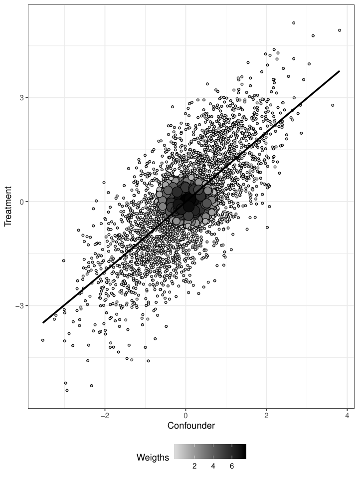
where is an unknown function that describe the relationship between the continuous treatment and the confounders (here, and are just two dummy variables). Equation (2.1) suggests finding weights that re-balance the joint distribution between treatment and confounders to be the same as that of the product of the two distributions. We now provide a straightforward example to clarify ideas. Figure 1 depicts the relationship between a normally distributed confounder with mean 0 and variance 1, and a normally distributed treatment with mean and unit variance. The straight line shows the relationship between the two while the dots represent the values obtained for the two variables. The darkness and the size of the circles represent the size of the weights, i.e., the darker/larger the circle, the larger the weight. A set of weights that minimize eq. (2.1), weights more those units with no relationship between the confounder and the continuous treatment making them orthogonal. In other words, the obtained weights eliminate any associations between the continuous treatment and the confounders, thus providing optimal covariate balance. As a matter of fact, recent literature on GPS-based methods (Austin 2019; Zhu et al. 2015) suggests the use of correlation-based diagnostics, such as the weighted correlation, to assess covariate balance. Our idea is not only to use this quantity as diagnostic but actually to find the set of weights that minimize it.
.
2.2 Worst-case penalized functional covariance
The functional covariance showed in equation 2.1, depends on the unknown function . In this Section, we propose to minimize the worst-case functional covariance normalized by the magnitude of the function . To do so, we start by embedding the function into a seminormed space with seminorm (a norm that can also assign the values and to nonzero elements), . We first define the normalized worst-case functional covariance as
| (2.2) |
which can be seen as the dual norm of the continuous linear operator, . In particular, we consider the norm given by an RKHS, a Hilbert space of functions which is associated with a positive semidefinite (PSD) kernel . Define the matrix as . Then, we have that
| (a) | |||||
| (b) | |||||
where is by the representer theorem (Schölkopf et al. 2001), and by the dual of the Euclidean norm, and is the vector with in every entry. This results shows that the worst case functional covariance can be expressed as a convex-quadratic function in . To control for extreme weights we propose to add a penalization term and consider the following worst-case penalized functional covariance,
When equals zero, we obtain weights that minimize the covariance. When is set to be large (depending on the data), we obtain uniform weights. We discuss choices of in Section 3. In the next Section, we show how to use quadratic optimization to minimize .
2.3 Quadratic optimization to minimize
In the previous Sections we introduced a functional formulation of the covariance between the continuous treatment and the confounders. Since this quantity depends on unknown function we considered the worst-case functional covariance, which is the dual norm of the continuous linear operator, , showed that it can be expressed as a convex-quadratic function in and defined the worst case penalized functional covariance, which aim at penalizing extreme weights. We restric the weights to be positive and sum up to one. Formally, we let . We propose to use weights obtained by solving the following optimization problem
| (2.3) |
As shown in Section 2.2, we can express as a convex-quadratic function in , and therefore, optimization problem (2.3) reduces to the following linearly-constrained convex-quadratic optimization problem,
| (2.4) |
where , , and is the diagonal matrix with in its diagonal entry.
2.4 Dose-response curve
In addition to the data presented in Section 2.1, for each unit in let be the potential outcome of treatment , and the observed outcome. The main object of inference in this paper is the dose-response curve . This quantity depends on unknown potential outcomes, and assumptions are needed to identify it in terms of observed data. In this paper we assume consistency, positivity and ignorability (Imbens and Rubin 2015). Consistency (together with non-interference) states that the observed outcome equals the potential outcome under the treatment applied to that specific unit, i.e., , and that the potential outcomes are well-defined. Positivity states that, the GPS is positive for all values of the confounders in their supports. Ignorability states that, once conditioned on the observed confounders, the potential outcomes are independent to the treatment assignment. Finally, under these assumption, it can be shown that the dose-response curve is identifiable using observational data.
In the previous Sections, we showed how to obtain weights that minimize the functional covariance defined in (2.1) by simply solving a linearly-constrained quadratic optimization problem. As described in Section 2.1, these weightseliminate any associations between the continuous treatment and the confounders, thus providing optimal covariate balance. Once these weights are obtained, to estimate the dose-response curve, we suggest plugging these weights into a weighted parametric or nonparametric estimator. For instance, similar to the approach of Naimi et al. 2014; Cole and Hernán 2008 for estimating marginal structural models, one can use a weighted nonlinear regression or a weighted local polynomial regression to estimate , regressing only the treatment on the outcome.
2.5 Properties
In this Section, we provide some insights on the properties of dose-response curve estimators weighted by KOOW weights. The overall idea of using weights that minimize the covariance between treatment and confounders has been previously studied in the context of maximal mean discrepancies (MMD) for density-ratio estimation or for testing independence of random variables (Sugiyama et al. 2012; Gretton et al. 2005). In addition, it is also been shown the connection between MMD and the more general Bregman divergence (see (Sugiyama et al. 2012, Section 7.3.2)). As a consequence, existing results can be used to describe the properties of our proposed methodology. Specifically, by following Sondhi et al. 2019; Menon and Ong 2016; Arbour and Dimmery 2019, using kernel functions (as in the local polynomial regression estimator) and under the assumption that exist a set of “true” weights that minimize the bias of the weighted estimator, e.g.., the stable inverse probability weights, we can bound the bias of the weighted estimator. For instance, the bias of the weighted estimator is bounded by the Bregman distance between the true weights and the weights obtained by solving the optimization problem plus a remainder of a smaller order than the bandwidth parameter when this term goes to infinity (Sondhi et al. 2019, Proposition 2). A similar bound is also provided for the variance (Sondhi et al. 2019, Proposition 3). Furthermore, Sondhi et al. 2019 show that under bounded variance, the weighted estimator is also consistent.
3 Practical guidelines
Solutions to the optimization problem (2.3) depend on the kernel specification, its hyperparameters and the penalization parameter . In this Section, we provide practical guidelines on their choice. We start by describing the choice of the kernel. Since we want to allow for a great level of flexibility in modeling the relationship between treatment and confounders, we suggest the use of a product of polynomial Mahalanobis kernels:
| (3.1) |
where
| (3.2) |
and where controls the overall scale of the kernel, is a parameter that controls the importance of higher orders degrees, is the sample covariance, is the sample mean, and is the parameter that controls the degree of the polynomial. Gretton et al. 2005 showed that by using universal kernels, such as the Gaussian and Matérn kernels, minimizing (2.3) leads to statistically independence, whereas by using non-universal kernels, such as polynomial kernels, we aim at uncorrelatedness. Although independence may be preferred over uncorrelatedness, we find that practically polynomial kernels suffice as shown in our simulations (Section 4) and in our illustration (Section 5) .
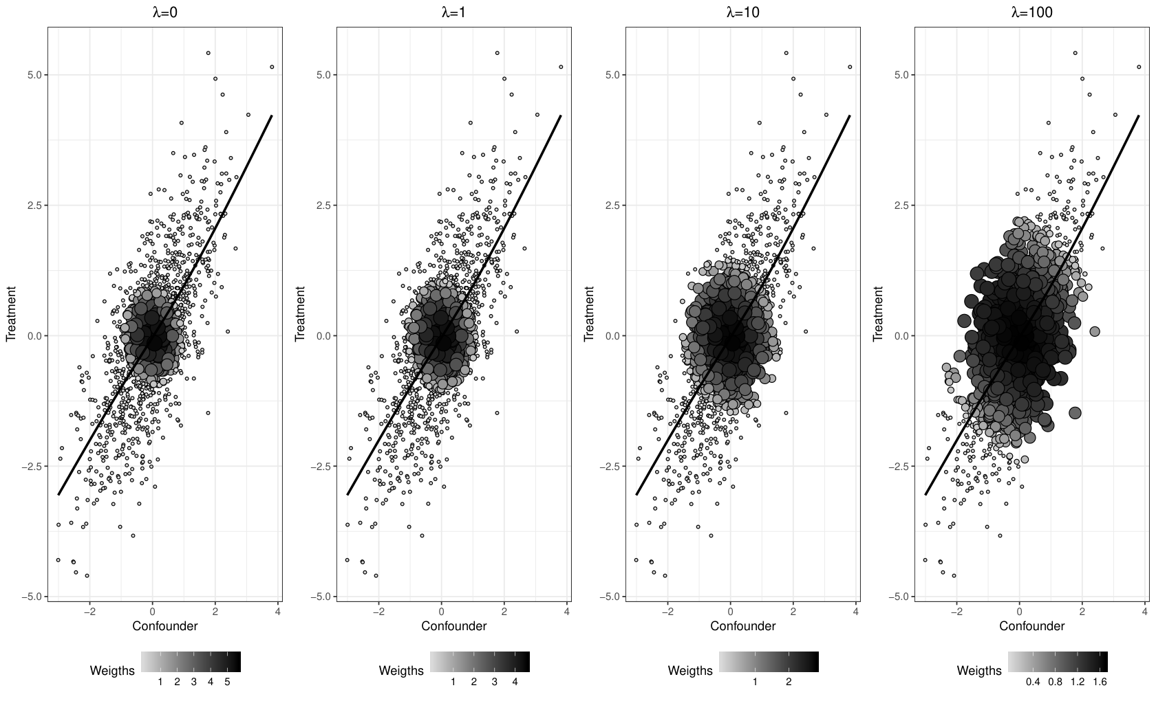
We now provide practical guidelines on how to tune the kernel’s hyperparameters and the penalization parameter . As shown by Kallus et al. 2018; Kallus and Santacatterina 2018, we suggest using marginal likelihood, a model selection criteria for Gaussian processes (Rasmussen and Nickisch 2010). To do so, we specify a Gaussian Process (GP) prior, with covariance identified by the product kernel , and suppose that we observed the potential outcome from with Gaussian noise of variance . We then maximize the marginal likelihood of seeing the data with respect to the hyperparameters, , , and . The penalization parameter can be interpreted as a uncorrelatedness-precision (bias-variance) trade-off parameter. When set to , the obtained weights targets minimal covariance and therefore minimal bias. When increases, the obtained weights have lower variance and higher precision can be consequently achieved. An example is provided in Figure 2, in which we plot the scatterplots between a confounder (X-axes) and a treatment (Y-axes) weighted by the set of weights obtained by solving the optimization problem (2.3), setting equal to 0 (first panel from the left of Figure 2), 1 (second panel), 10 (third panel) and 100 (fourth panel). When increasing the penalization parameter , it is clear from this Figure that the distribution of the weights become more uniform (bottom of each scatterplot) thus achieving less uncorrelatedness but increasing precision. In practical setting, an acceptable level of penalization, and therefore of precision, may be for the analyst to determine. We suggest, starting by lower values and, in case, trying to explore different values within reason. We show this in our simulations in Section 4.
To estimate standard errors of the dose-response curve, we suggest using bootstrap. Specifically, we suggest to bootstrap the whole process, namely the estimation of the weights, and that of the dose-response curve by a weighted estimator, as shown in our simulation study.
To tune hyperparameters and solve linearly-constrained convex-quadratic optimization problems several software can be used. We suggest using the GaussianProcessRegressor package from scikit-learn (Pedregosa et al. 2011) for tuning the hyperparameters and Gurobi (Gurobi Optimization 2014) for solving quadratic optimization problems.
4 Simulations
In this Section, we present the results of a simulation study aimed at evaluating the performance, in terms of integrated absolute bias (IAB) and integrated root mean squared error (IRMSE) across several simulation scenarios. In summary, KOOW performed well with respect to integrated absolute bias and integrated root mean squared error, across the considered scenarios and regardless of the use of a parametric or a nonparametric model for the dose-response curve.
4.1 Setup
We considered a sample size of . We generated
and considered three scenarios for the treatment mechanism: linear, quadratic and cubic. Specifically, we generated
where and , for the linear, quadratic and cubic scenario, respectively, and , . We generated the true dose-response curves by evaluating the true models at a grid of 1,000 values from -3 to 3.
We compared KOOW with, outcome modeling (OM) (Flores et al. 2007), the non parametric doubly robust estimator of Kennedy et al. 2017 (NPDR), matching on the generalized propensity score (CM) (Wu et al. 2018), (stable) inverse probability of treatment weighting (IPW) (Naimi et al. 2014), parametric (CBPS) and nonparametric covariate balancing propensity score (npCBPS) (Fong et al. 2018). We used Super Learner (Van der Laan et al. 2007) to model the relationships between the outcome the treatment and the confounders (the outcome model) and to model the relationship between the continuous treatment and the confounders (treatment model) for OM, NPDR, and IPW. We considered the following list of algorithms for the Super Learner: linear model, linear model with interactions, linear model with lasso penalization, generalized additive models, multivariate adaptive regression splines, bayesian linear model, and local polynomial regression. For KOOW, we considered and .
We estimated the dose-response curve by using a local polynomial regression estimator with degree 2 and a cubic parametric regression estimator for all methods. Specifically, for KOOW, IPW, CBPS, and npCBPS we plugged the obtained weights into the local polynomial and cubic parametric regression estimators. For OM, NPDR, and CM, we regressed the treatment on the “pseudo” outcomes. We compared KOOW with the other methods with respect to IAB and IRMSE defined as in (Kennedy et al. 2017; Wu et al. 2018, Section 4 and Section 5.1, respectively). We used scikit-learn (via the R package reticulate) to tune the hyperparametes of the GPs, the R interface of Gurobi to obtain the set of KOOW weights, the R package SuperLearner for computing the outcome and treatment models, and the R package loess and glm for local polynomial and cubic parametric regression estimation.
4.2 Results
In this Section we discuss the results of our simulation study. In summary, KOOW performed well with respect to IAB and IRMSE across all three considered scenarios and regardeless of the model used to estimate the dose-response curve (local polynomial or cubic regression). Specifically, as shown in Table 1, when using a local polynomial regression model, KOOW () obtained the lowest IAB across all scenarios. While OM, NPDR and IPW performed well with respect to IAB and IRMSE under the linear scenario (linear treatment mechanism - first column of Table 1), their performance deteriorated when increasing the complexity of the treatment mechanism (second and third columns of Table 1). For instance, NPDR had an IAB of 0.49 under the linear scenario, increasing to 3.18 in the quadratic scenario and to 50.58 in the cubic scenario. CM performed relatively well only in the quadratic scenario. CBPS and npCBPS performed well across the three scenarios, suggesting that methods that target balance may have good performance when estimating the effects of continuous treatments. It is worth mentioning that across all scenarios, the IAB of KOOW slightly increased when increasing the penalization parameter , while the IRMSE significantly decreased. This suggests that KOOW was able to improve precision while introducing negligible bias by penalization.
We obtained similar results for KOOW, OM, NPDR, IPW and CM when estimating the dose-response curve with a cubic parametric model (Table 2). CBPS and npCBPS performed worse compared to themselves when estimating the dose-response curve with a local polynomial regression. The IAB of KOOW in the quadratic scenario (second colum of Table 2) decreased while increasing the penalization parameter from to which is in contrast to the results of all the other scenarios. We argue that this result is related to this specific scenario and is heuristically explained by the fact that increasing precision by penalization leads to less erroneous estimates and consequently less biased results. Figures 5,6,7 in the Supplementary Material show boxplots of the estimated linear (top-left panels), quadratic (top-right panels), and cubic (bottom-left panels) coefficients of the cubic parametric model for the dose-response curve around their true values (horizontal lines) for all the methods and across scenarios (linear, quadratic and cubic). As suggested by the results in Table 2, KOOW, performed well across scenarios and for all coefficients. Specifically, the interquantile ranges of KOOW’s boxplots almost always included the true coefficient.
| Treatment mechanism | |||
|---|---|---|---|
| Linear | Quadratic | Cubic | |
| IAB (IRMSE) | |||
| Methods | |||
| KOOW | 0.46 (2.25) | 0.19 (2.83) | 0.34 (1.97) |
| KOOW | 0.51 (1.93) | 0.21 (2.25) | 0.38 (1.75) |
| KOOW | 0.67 (1.50) | 0.23 (1.38) | 0.59 (1.36) |
| OM | 1.32 (1.48) | 4.54 (5.78) | 17.07 (35.28) |
| NPDR | 0.49 (0.94) | 3.18 (4.74) | 50.58 (157.58) |
| IPW | 0.50 (2.04) | 0.37 (1.06) | 3.87 (4.55) |
| CM | 9.75 (10.80) | 1.64 (5.78) | 27.67 (28.14) |
| CBPS | 0.67 (4.56) | 0.44 (0.79) | 0.56 (2.62) |
| npCBPS | 0.98 (2.61) | 0.73 (1.00) | 1.53 (2.43) |
-
Notes: KOOW refers to Kernel Optimal Orthogonality Weighting where is the penalization parameter; OM refers to Outcome Modeling; NPDR refers to Non Parametric Doubly Robust; IPW to (stable) Inverse Probability Weighting; CM to caliper matching for continuous treatment; CBPS and npCBPS to parametric and non parametric Covariate Balancing Propensity Score. We used Super Learner to model the outcome and treatment models for NPDR, IPW and OM.
| Treatment mechanism | |||
|---|---|---|---|
| Linear | Quadratic | Cubic | |
| IAB (IRMSE) | |||
| Methods | |||
| KOOW | 0.46 (2.44) | 0.28 (4.88) | 0.13 (2.23) |
| KOOW | 0.51 (2.10) | 0.10 (3.46) | 0.15 (1.95) |
| KOOW | 0.71 (1.61) | 0.07 (1.95) | 0.27 (1.48) |
| OM | 2.93 (3.00) | 4.53 (5.78) | 20.26 (36.01) |
| NPDR | 0.14 (1.00) | 1.01 (5.92) | 7.36 (72.98) |
| IPW | 1.77 (3.36) | 0.89 (3.94) | 3.85 (4.90) |
| CM | 1.55 (8.41) | 4.99 (34.48) | 42.80 (44.92) |
| CBPS | 2.51 (5.46) | 3.24 (7.04) | 3.15 (5.81) |
| npCBPS | 6.98 (7.67) | 1.51 (7.16) | 12.45 (12.66) |
-
Notes: KOOW refers to Kernel Optimal Orthogonality Weighting where is the penalization parameter; OM refers to Outcome Modeling; NPDR refers to Non Parametric Doubly Robust; IPW to (stable) Inverse Probability Weighting; CM to caliper matching for continuous treatment; CBPS and npCBPS to parametric and non parametric Covariate Balancing Propensity Score. We used Super Learner to model the outcome and treatment models for NPDR, IPW and OM.
5 Case-study
In this Section, we apply KOOW to the evaluation of the effect of red meat consumption on blood pressure among women of the Women’s Health Initiative (WHI) observational study.
5.1 The effect of red meat consumption on hypertension among women of the WHI observational study
Despite increasing efforts to early detect and treat high blood pressure in recent years, hypertension still remains one of the major risk factor for stroke, cardiovascular diseases and mortality worldwide (Wang and Wang 2004; Lawes et al. 2006; Collaboration et al. 2002). In the eighties, the “iron-heart” hypothesis (Sullivan 1981) was proposed to explain possible differences in rates of coronary heart disease between pre-menopausal women and men. This hypothesis, was based on the idea that pre-menopausal women loose iron through menstruation. Since these results, several studies have evaluated the relationship between iron and coronary heart disease suggesting that greater haem iron (the iron originated from animal sources) intake increases the risk of coronary heart disease (Wang et al. 2016, for a recent meta-analysis). Red meat is a major source of haem iron and several studies and guidelines suggest consuming a modest amount of red meat. Most of these studies categorize red meat consumption in two or few categories and evaluate their effects on a binary outcome, such as presence or not of hypertension (see Kappeler et al. 2013 for example). However, as described in Section 1, a more natural object of interest is the dose-response curve, which directly evaluates the amount of red meat that a person eats every day on a continuous outcome. Therefore, in this Section we apply KOOW to estimate the dose-response curve of red meat consumption and systolic blood pressure.
5.2 Study population
We used a subset of 2,000 randomly selected units from the the Women’s Health Initiative (WHI) observational study (Study et al. 1998). WHI is one of the largest cohort of postmenopausal women aged 50 to 79 years that provides valuable information about demographic and clinical information such as data on blood pressure and hormone therapy treatment. Red meat consumption was recorded as estimated medium servings per day. We restricted our analyses to those women between the 5th and the 95th quantile of the distribution of red meat consumption. Thus, the minimum medium red meat serving per day in our subset was equal to 0.04, the mean 0.53, and the maximum 1.51. We identified as potential confounders the following variables: systolic blood pressure at baseline, age, total dietary energy intake (measure in kcal), body mass index (BMI) (calculated as weight in kilograms divided by the square of height in meters), smoking status (defined as if a woman ever smoked at least 100 cigarettes), and hormone therapy (HT) ever used (defined as if a woman ever used HT).
5.3 Model setup
We obtained the set of KOOW weights by solving optimization problem 2.3. We set equal to 10. We chose a product of two polynomial kernel degree 1, and we tuned their hyperparameters by using GPML as described in Section 4. We estimated the dose-response curve by using a local polynomial regression estimator degree 1 weighted by the set of KOOW weights. We bootstrapped the whole process of obtaining the KOOW weights and estimating the dose-response curve, 1000 times. For each bootstrap sample, we computed the predicted dose-response curve and finally estimated its bootstrap confidence interval.
5.4 Results
In this Section we present the results of our analysis. Similar to the results of previous studies we show a possible association between red meat consumption and hypertension. Figure 3, shows the dose response curve between red meat consumption (x-axis) and the systolic blood pressure (y-axis). Mean systolic blood pressure was around 125 for those women with low medium red meat consumption, while increasing, up to almost 175, along with the consumption of red meat. The top left panel of Figure 4 shows adjusted, i.e.., weighted by the KOOW weights, covariate balance (black dots) and unadjusted (grey dots) of the six confounders considered in our analysis. Covariate balance was computed as the absolute weighted correlation between the continuous treatment and the confounders. KOOW shows to minimize covariate balance to values close to 0. Figure 4 also shows the scatterplots between each of the six considered confounders (x-axes of the top right panel and the middle and bottom panels of Figure 4), and red meat consumption (y-axes). As shown in Figure 1 in Section 2.1, KOOW provide weights that make confounders and red meat consumption orthogonal. For completeness we also report the weighted units for the binary confounders smoked and hormone therapy in the bottom panels of Figure 4. Finally, based on the results of our analysis and similar to previous epidemiological and medical literature, we conclude that there may be a possible positive relationship between red meat consumption and systolic blood pressure.

6 Conclusion
Continuous treatments arises very often in practice and proper estimation of dose-response curves is crucial for medical decision making. In this paper we proposed a novel method based on quadratic optimization that finds weights that minimize the covariance between the continuous treatment and the confounders, thus eliminating any possible relationships between the two and consequently optimizing covariate balance.
By using kernels, the proposed method automatically learns the structure of the data without relying on parametric assumptions about the outcome model, which, in most practical settings, are hardly ever met. In addition, as shown in Section 3, the penalization parameter can be easily tuned and interpreted as the uncorrelatedness-precision (bias-variance) trade-off parameter. The proposed method provided low integrated absolute bias and low integrated RMSE across several different scenario, as showed in our simulation scenarios,
In this paper, we tuned the kernels’ hyperparametes by using Gaussian Process Marginal Likelihood. Other methods may be also used. For instance, one can use a kernelized regression and tune the kernels hyperparameters by usual cross validation techniques.
In this paper, once the set of weights was obtained, we plugged it into a weighted estimator for the dose-response curve. Alternative weighted estimation techniques may also be considered. For instance, one may first estimate the KOOW weights and the plug them into a parametric or nonparametric augmented estimator, similar to that of Kennedy et al. 2017. Another option would be to use a KOOW-weighted regression estimator that includes both treatment and confounders as in (Kang et al. 2007, Section 3.2).
References
- Alejo et al. (2018) Alejo, J., A. F. Galvao, and G. Montes-Rojas (2018). Quantile continuous treatment effects. Econometrics and statistics 8, 13–36.
- Arbour and Dimmery (2019) Arbour, D. and D. Dimmery (2019, Jan). Permutation Weighting. arXiv e-prints, arXiv:1901.01230.
- Austin (2019) Austin, P. C. (2019). Assessing covariate balance when using the generalized propensity score with quantitative or continuous exposures. Statistical methods in medical research 28(5), 1365–1377.
- Barrett et al. (2014) Barrett, J. K., R. Henderson, and S. Rosthøj (2014). Doubly robust estimation of optimal dynamic treatment regimes. Statistics in biosciences 6(2), 244–260.
- Bia et al. (2011) Bia, M., C. A. Flores, and A. Mattei (2011). Nonparametric estimators of dose-response functions. CEPS/INSTEAD Working Paper Series 40, 2011–40.
- Cole and Hernán (2008) Cole, S. R. and M. A. Hernán (2008). Constructing inverse probability weights for marginal structural models. American journal of epidemiology 168(6), 656–664.
- Collaboration et al. (2002) Collaboration, P. S. et al. (2002). Age-specific relevance of usual blood pressure to vascular mortality: a meta-analysis of individual data for one million adults in 61 prospective studies. Lancet 360(9349), 1903–1913.
- Demirer et al. (2019) Demirer, M., V. Syrgkanis, G. Lewis, and V. Chernozhukov (2019). Semi-parametric efficient policy learning with continuous actions. arXiv preprint arXiv:1905.10116.
- d’Haultfoeuille et al. (2013) d’Haultfoeuille, X., S. Hoderlein, and Y. Sasaki (2013). Nonlinear difference-indifferences in repeated cross sections with continuous treatments. Technical report, cemmap working paper, Centre for Microdata Methods and Practice.
- Florens et al. (2008) Florens, J.-P., J. J. Heckman, C. Meghir, and E. Vytlacil (2008). Identification of treatment effects using control functions in models with continuous, endogenous treatment and heterogeneous effects. Econometrica 76(5), 1191–1206.
- Flores et al. (2007) Flores, C. A. et al. (2007). Estimation of dose-response functions and optimal doses with a continuous treatment. University of Miami. Typescript.
- Fong et al. (2018) Fong, C., C. Hazlett, K. Imai, et al. (2018). Covariate balancing propensity score for a continuous treatment: application to the efficacy of political advertisements. The Annals of Applied Statistics 12(1), 156–177.
- Galvao and Wang (2015) Galvao, A. F. and L. Wang (2015). Uniformly semiparametric efficient estimation of treatment effects with a continuous treatment. Journal of the American Statistical Association 110(512), 1528–1542.
- Gill (2004) Gill, R. D. (2004). Causal inference for complex longitudinal data: The continuous time g-computation formula. arXiv preprint math/0409436.
- Gill and Robins (2001) Gill, R. D. and J. M. Robins (2001). Causal inference for complex longitudinal data: the continuous case. Annals of Statistics, 1785–1811.
- Gretton et al. (2007) Gretton, A., K. Borgwardt, M. Rasch, B. Schölkopf, and A. J. Smola (2007). A kernel method for the two-sample-problem. In Advances in neural information processing systems, pp. 513–520.
- Gretton et al. (2005) Gretton, A., R. Herbrich, A. Smola, O. Bousquet, and B. Schölkopf (2005). Kernel methods for measuring independence. Journal of Machine Learning Research 6(Dec), 2075–2129.
- Gretton et al. (2009) Gretton, A., A. Smola, J. Huang, M. Schmittfull, K. Borgwardt, and B. Schölkopf (2009). Covariate shift by kernel mean matching. Dataset shift in machine learning 3(4), 5.
- Gurobi Optimization (2014) Gurobi Optimization (2014). Gurobi optimizer reference manual. Google Scholar.
- Hill (2011) Hill, J. L. (2011). Bayesian nonparametric modeling for causal inference. Journal of Computational and Graphical Statistics 20(1), 217–240.
- Hirano and Imbens (2004) Hirano, K. and G. W. Imbens (2004). The propensity score with continuous treatments. Applied Bayesian modeling and causal inference from incomplete-data perspectives 226164, 73–84.
- Huang et al. (2007) Huang, J., A. Gretton, K. Borgwardt, B. Schölkopf, and A. J. Smola (2007). Correcting sample selection bias by unlabeled data. In Advances in neural information processing systems, pp. 601–608.
- Imai and Van Dyk (2004) Imai, K. and D. A. Van Dyk (2004). Causal inference with general treatment regimes: Generalizing the propensity score. Journal of the American Statistical Association 99(467), 854–866.
- Imbens and Rubin (2015) Imbens, G. W. and D. B. Rubin (2015). Causal inference in statistics, social, and biomedical sciences. Cambridge University Press.
- Kallus et al. (2018) Kallus, N., B. Pennicooke, and M. Santacatterina (2018). More robust estimation of sample average treatment effects using kernel optimal matching in an observational study of spine surgical interventions. arXiv preprint arXiv:1811.04274.
- Kallus and Santacatterina (2018) Kallus, N. and M. Santacatterina (2018). Optimal balancing of time-dependent confounders for marginal structural models. arXiv preprint arXiv:1806.01083.
- Kallus and Zhou (2018) Kallus, N. and A. Zhou (2018). Policy evaluation and optimization with continuous treatments. arXiv preprint arXiv:1802.06037.
- Kang et al. (2007) Kang, J. D., J. L. Schafer, et al. (2007). Demystifying double robustness: A comparison of alternative strategies for estimating a population mean from incomplete data. Statistical science 22(4), 523–539.
- Kappeler et al. (2013) Kappeler, R., M. Eichholzer, and S. Rohrmann (2013). Meat consumption and diet quality and mortality in nhanes iii. European journal of clinical nutrition 67(6), 598.
- Kennedy et al. (2017) Kennedy, E. H., Z. Ma, M. D. McHugh, and D. S. Small (2017). Non-parametric methods for doubly robust estimation of continuous treatment effects. Journal of the Royal Statistical Society: Series B (Statistical Methodology) 79(4), 1229–1245.
- Kreif et al. (2015) Kreif, N., R. Grieve, I. Díaz, and D. Harrison (2015). Evaluation of the effect of a continuous treatment: A machine learning approach with an application to treatment for traumatic brain injury. Health economics 24(9), 1213–1228.
- Krishnamurthy et al. (2019) Krishnamurthy, A., J. Langford, A. Slivkins, and C. Zhang (2019). Contextual bandits with continuous actions: Smoothing, zooming, and adapting. arXiv preprint arXiv:1902.01520.
- Lawes et al. (2006) Lawes, C. M., S. Vander Hoorn, M. R. Law, P. Elliott, S. MacMahon, and A. Rodgers (2006). Blood pressure and the global burden of disease 2000. part ii: estimates of attributable burden. Journal of hypertension 24(3), 423–430.
- Lu et al. (2011) Lu, B., R. Greevy, X. Xu, and C. Beck (2011). Optimal nonbipartite matching and its statistical applications. The American Statistician 65(1), 21–30.
- Lu et al. (2001) Lu, B., E. Zanutto, R. Hornik, and P. R. Rosenbaum (2001). Matching with doses in an observational study of a media campaign against drug abuse. Journal of the American Statistical Association 96(456), 1245–1253.
- Menon and Ong (2016) Menon, A. and C. S. Ong (2016). Linking losses for density ratio and class-probability estimation. In International Conference on Machine Learning, pp. 304–313.
- Moodie and Stephens (2012) Moodie, E. E. and D. A. Stephens (2012). Estimation of dose–response functions for longitudinal data using the generalised propensity score. Statistical methods in medical research 21(2), 149–166.
- Naimi et al. (2014) Naimi, A. I., E. E. Moodie, N. Auger, and J. S. Kaufman (2014). Constructing inverse probability weights for continuous exposures: a comparison of methods. Epidemiology 25(2), 292–299.
- Neugebauer and van der Laan (2006) Neugebauer, R. and M. J. van der Laan (2006). G-computation estimation for causal inference with complex longitudinal data. Computational Statistics & Data Analysis 51(3), 1676–1697.
- Pedregosa et al. (2011) Pedregosa, F., G. Varoquaux, A. Gramfort, V. Michel, B. Thirion, O. Grisel, M. Blondel, P. Prettenhofer, R. Weiss, V. Dubourg, J. Vanderplas, A. Passos, D. Cournapeau, M. Brucher, M. Perrot, and E. Duchesnay (2011). Scikit-learn: Machine learning in Python. Journal of Machine Learning Research 12, 2825–2830.
- Rasmussen and Nickisch (2010) Rasmussen, C. E. and H. Nickisch (2010). Gaussian processes for machine learning (gpml) toolbox. Journal of Machine Learning Research 11(Nov), 3011–3015.
- Robins (1986) Robins, J. (1986). A new approach to causal inference in mortality studies with a sustained exposure period—application to control of the healthy worker survivor effect. Mathematical modelling 7(9-12), 1393–1512.
- Robins (2000) Robins, J. M. (2000). Marginal structural models versus structural nested models as tools for causal inference. In Statistical models in epidemiology, the environment, and clinical trials, pp. 95–133. Springer.
- Santacatterina and Bottai (2018) Santacatterina, M. and M. Bottai (2018). Optimal probability weights for inference with constrained precision. Journal of the American Statistical Association 113(523), 983–991.
- Schölkopf et al. (2001) Schölkopf, B., R. Herbrich, and A. J. Smola (2001). A generalized representer theorem. In International conference on computational learning theory, pp. 416–426. Springer.
- Sondhi et al. (2019) Sondhi, A., D. Arbour, and D. Dimmery (2019). Balanced off-policy evaluation general action spaces. arXiv preprint arXiv:1906.03694.
- Study et al. (1998) Study, T. W. H. I. et al. (1998). Design of the women’s health initiative clinical trial and observational study. Controlled clinical trials 19(1), 61–109.
- Sugiyama et al. (2012) Sugiyama, M., T. Suzuki, and T. Kanamori (2012). Density ratio estimation in machine learning. Cambridge University Press.
- Sullivan (1981) Sullivan, J. (1981). Iron and the sex difference in heart disease risk. The Lancet 317(8233), 1293–1294.
- Van Der Laan and Dudoit (2003) Van Der Laan, M. J. and S. Dudoit (2003). Unified cross-validation methodology for selection among estimators and a general cross-validated adaptive epsilon-net estimator: Finite sample oracle inequalities and examples.
- Van der Laan et al. (2007) Van der Laan, M. J., E. C. Polley, and A. E. Hubbard (2007). Super learner. Statistical applications in genetics and molecular biology 6(1).
- Wang et al. (2016) Wang, X., X. Lin, Y. Y. Ouyang, J. Liu, G. Zhao, A. Pan, and F. B. Hu (2016). Red and processed meat consumption and mortality: dose–response meta-analysis of prospective cohort studies. Public health nutrition 19(5), 893–905.
- Wang and Wang (2004) Wang, Y. and Q. J. Wang (2004). The prevalence of prehypertension and hypertension among us adults according to the new joint national committee guidelines: new challenges of the old problem. Archives of internal medicine 164(19), 2126–2134.
- World Research Cancer Fund (2018) World Research Cancer Fund, A. I. f. C. R. (2018). Recommendations and public health and policy implications. Continuous update project experts.
- Wu et al. (2018) Wu, X., F. Mealli, M.-A. Kioumourtzoglou, F. Dominici, and D. Braun (2018). Matching on generalized propensity scores with continuous exposures. arXiv preprint arXiv:1812.06575.
- Xiao et al. (2013) Xiao, Y., E. E. Moodie, and M. Abrahamowicz (2013). Comparison of approaches to weight truncation for marginal structural cox models. Epidemiologic Methods 2(1), 1–20.
- Yiu and Su (2018) Yiu, S. and L. Su (2018). Covariate association eliminating weights: a unified weighting framework for causal effect estimation. Biometrika 105(3), 709–722.
- Zhang et al. (2016) Zhang, Z., J. Zhou, W. Cao, and J. Zhang (2016). Causal inference with a quantitative exposure. Statistical methods in medical research 25(1), 315–335.
- Zhu et al. (2015) Zhu, Y., D. L. Coffman, and D. Ghosh (2015). A boosting algorithm for estimating generalized propensity scores with continuous treatments. Journal of causal inference 3(1), 25–40.
SUPPLEMENTARY MATERIAL
- Simulations:
-
Additional Figures5,6,7 showing the boxplots of the estimated linear (top-left panels),quadratic (top-right panels), and cubic (bottom-left panels) coefficients of the cubic para-metric model for the dose-response curve around their true values (horizontal lines) for all the methods and across scenario.