跳到论文正文
W Papers独立论文阅读器 arXiv:1910.11864 论文正文 计算阅读时间 · 0%
引用这篇论文根据当前论文元数据生成,正式投稿前建议核对。


License: arXiv.org perpetual non-exclusive license
arXiv:1910.11864v1 [math.DS] 25 Oct 2019

Existence and spectral stability of multi-pulses in discrete Hamiltonian lattice systems

Ross Parker Email: ross_parker@brown.edu Address: Division of Applied Mathematics, Brown University, Providence, RI 02912, USA    P. G. Kevrekidis Email: kevrekid@math.umass.edu Address: Department of Mathematics and Statistics, University of Massachusetts, Amherst MA 01003, USA Address: Mathematical Institute, University of Oxford, Oxford, OX2 6GG, UK    Björn Sandstede Email: bjorn_sandstede@brown.edu Address: Division of Applied Mathematics, Brown University, Providence, RI 02912, USA
Abstract

In the present work, we consider the existence and spectral stability of multi-pulse solutions in Hamiltonian lattice systems. We provide a general framework for the study of such wave patterns based on a discrete analogue of Lin’s method, previously used in the continuum realm. We develop explicit conditions for the existence of mm-pulse structures and subsequently develop a reduced matrix allowing us to address their spectral stability. As a prototypical example for the manifestation of the details of the formulation, we consider the discrete nonlinear Schrödinger equation. Different families of 22- and 33-pulse solitary waves are discussed, and analytical expressions for the corresponding stability eigenvalues are obtained which are in very good agreement with numerical results.

Keywords: 
discrete NLS equation , lattice differential equations , Lin’s method
MSC
39A30, 37K60

1 Introduction and motivation

The study of multi-pulse wave structures has a time honored history in continuum systems. Attempts at a systematic formulation have taken place both at a more phenomenological, asymptotic level [7] and at a more rigorous level [27]. The development in the latter work of the so-called Lin’s method for such wave patterns offered a systematic view into a reduced formulation where the characteristics of the pulses (such as their centers, or possibly also their widths) could constitute effective dynamical variables for which simpler dynamical equations, i.e. ordinary differential equations, could be derived. While Lin’s method for discrete dynamical systems has been developed in [18], it has not so far been applied to the discrete multi-pulse problem. Over the following decade, methods were sought to isolate and freeze the dynamics of individual pulses within the patterns [4, 3]. More recently, such freezing techniques have also been extended to other structures including rotating waves [5].

Despite the intense interest in such multiple coherent structure patterns at the continuum limit, similar techniques have not been systematically developed at the discrete level. Parts of the relevant efforts have involved an attempt at adapting the asymptotic methodology of [7] (in the work of [16]) and also the consideration of structures systematically in the vicinity of the so-called anti-continuum limit [22]. The latter setting involves as a starting point the limit of vanishing coupling between the discrete sites, whereby suitable Lyapunov-Schmidt conditions can be brought to bear to identify persistent configurations for finite coupling strengths between the adjacent lattice sites. While works such as [13] have emerged that develop instability criteria, it would be useful to have a systematic toolbox to study the spectrum of multi-pulses in the spatially discrete setting. This would serve to both quantify the persistence conditions of the multi-structure states, and also to offer specific predictions on their spectral stability and nonlinear dynamics.

It is this void that it is the aim of the present work to fill. We start from a general formulation of Lin’s method for the discrete multi-pulse problem in Hamiltonian systems. (For non-Hamiltonian systems, an adaptation of the results in [27] is also possible). Assuming that a homoclinic orbit exists (the single pulse), we systematically develop conditions for the persistence of multi-pulse states. We then provide estimates of their relevant stability eigenvalues for the low dimensional (reduced) system of the pulses. These eigenvalues are close to 0, and we call them interaction eigenvalues, since they result from nonlinear interaction between neighboring copies of the primary pulse.

As a concrete example for the implementation of the method, we revisit the discrete nonlinear Schrödinger (DNLS) system for which many of the methods of the previous paragraph have been developed [17] (see also [23]). In particular, we give a systematic description especially of 2- and 3-pulse solutions and explain how the relevant conclusions can be generalized to arbitrary multi-pulse structures. Our presentation will be structured as follows. In section 2, we will present the mathematical setup of the problem and of the special case (DNLS) example of interest. In section 3, we will develop Lin’s method providing the main results but deferring the proof details to later sections. In section 4, we apply the method to the DNLS, comparing the theoretical findings to systematic computations of multi-pulse solutions. Our results are then summarized and some possible directions for future work are offered. Details of the proofs are presented in sections 6-8.

2 Mathematical setup

A lattice dynamical system is an infinite system of ordinary differential equations which are indexed by points (nodes) on a lattice. For the purposes of this work, we will only consider dynamical systems on the integer lattice ℤ{\mathbb{Z}}, where the differential equation for each point on the lattice is identical, and the equations are coupled by a centered, second order difference operator.

As a specific example, we will look at the discrete nonlinear Schrödinger equation (DNLS)

i​ψ˙n+d⁡(ψn+1−2​ψn+ψn−1)+|ψn|2​ψn=0,i\dot{\psi}_{n}+d(\psi_{n+1}-2\psi_{n}+\psi_{n-1})+|\psi_{n}|^{2}\psi_{n}=0, (1)

which is (2.12) in [17], where we have taken β=−1\beta=-1 and σ=1\sigma=1. The parameter dd represents the coupling between nodes; d>0d>0 is the focusing case, and d<0d<0 the defocusing case [17]. Equation Eq. 1 is Hamiltonian, with energy given by (2.17) in [17, 23]. Of general interest in this type of lattice is the existence and stability of standing waves, which are bound state solutions of the form ψn​(t)=ei​ω​t​ϕn\psi_{n}(t)=e^{i\omega t}\phi_{n} [1]. Making this substitution in Eq. 1 and simplifying, a standing wave solves the steady state equation

d⁡(ϕn+1−2​ϕn+ϕn−1)−ω​ϕn+|ϕn|2​un=0.d(\phi_{n+1}-2\phi_{n}+\phi_{n-1})-\omega\phi_{n}+|\phi_{n}|^{2}u_{n}=0. (2)

From [10], a symmetric, real-valued, on-site soliton solution qnq_{n} exists to Eq. 2 for all ω≠0\omega\neq 0 and d≥0d\geq 0. This solution qnq_{n} furthermore is differentiable in ω\omega.

We will write DNLS as a system of two real variables u=(v,w)∈ℓ2​(ℤ,ℝ2)u=(v,w)\in\ell^{2}({\mathbb{Z}},{\mathbb{R}}^{2}), where v=Re ​ψv=\text{Re }\psi and w=Im ​ψw=\text{Im }\psi. In this fashion, we can write Eq. 1 in Hamiltonian form as

u˙n+J​[ℋ′​(u)]n=0,\dot{u}_{n}+J[\mathcal{H}^{\prime}(u)]_{n}=0, (3)

where JJ is the standard skew-symmetric symplectic matrix

J=(01−10)J=\begin{pmatrix}0&1\\ -1&0\end{pmatrix}

and the Hamiltonian ℋ:ℓ2​(ℤ,ℝ2)→ℝ\mathcal{H}:\ell^{2}({\mathbb{Z}},{\mathbb{R}}^{2})\rightarrow{\mathbb{R}} is

ℋ(v,w)=−∑n=−∞∞(d2(vn−vn−1)2+d2(wn−wn−1)2−14(vn2+wn2)2).\mathcal{H}(v,w)=-\sum_{n=-\infty}^{\infty}\left(\frac{d}{2}\left(v_{n}-v_{n-1}\right)^{2}+\frac{d}{2}\left(w_{n}-w_{n-1}\right)^{2}-\frac{1}{4}\left(v_{n}^{2}+w_{n}^{2}\right)^{2}\right). (4)

The Hamiltonian ℋ\mathcal{H} is invariant under the standard rotation group R⁡(θ)R(\theta), given by

R⁡(θ)=(cos⁡(θ)sin⁡(θ)−sin⁡(θ)cos⁡(θ)),R(\theta)=\begin{pmatrix}\cos(\theta)&\sin(\theta)\\ -\sin(\theta)&\cos(\theta)\end{pmatrix}, (5)

which has infinitesimal generator R′​(0)=JR^{\prime}(0)=J. In addition, there is another conserved quantity, often called the norm or the power of the solution, which is given by

𝒬⁡(v,w)=12​∑n=−∞∞(vn2+wn2).\mathcal{Q}(v,w)=\frac{1}{2}\sum_{n=-\infty}^{\infty}\left(v_{n}^{2}+w_{n}^{2}\right). (6)

Standing waves are solutions of Eq. 3 of the form R⁡(ω​t)​uR(\omega t)u, where uu is independent of tt. Substituting this into Eq. 3, we obtain the equivalent system of equations

ℋ′​(u)−ω​u=0,\mathcal{H}^{\prime}(u)-\omega u=0, (7)

which for DNLS is given by

d⁡(vn+1−2​vn+vn−1)+vn​wn2+vn3−ω​vn\displaystyle d(v_{n+1}-2v_{n}+v_{n-1})+v_{n}w_{n}^{2}+v_{n}^{3}-\omega v_{n} =0\displaystyle=0 (8)
d⁡(wn+1−2​wn+wn−1)+vn2​wn+wn3−ω​wn\displaystyle d(w_{n+1}-2w_{n}+w_{n-1})+v_{n}^{2}w_{n}+w_{n}^{3}-\omega w_{n} =0.\displaystyle=0\>.

If uu is a standing wave solution, then R⁡(θ)​uR(\theta)u is also a standing wave by symmetry. We note that the steady state system has the form

ℋ′​(u)−ω​𝒬′​(u)=0,\mathcal{H}^{\prime}(u)-\omega\mathcal{Q}^{\prime}(u)=0, (9)

which is the stationary equation [9, (2.15)]. The steady state equation Eq. 8 also has a conserved quantity EE [12], which is given by

E=2​d​(vn​wn−1−vn−1​wn)=2​d​⟨un,J​un−1⟩.E=2d(v_{n}w_{n-1}-v_{n-1}w_{n})=2d\langle u_{n},Ju_{n-1}\rangle. (10)

By a conserved quantity in this setting we mean that this quantity is independent of the lattice index nn.

For stability analysis, the linearization of Eq. 3 about a standing wave solution u∗u^{*} yields the linear operator L⁡(u∗)L(u^{*}), given by

L⁡(u∗)=J​ℋ′′​(u∗)−ω​J.L(u^{*})=J\mathcal{H}^{\prime\prime}(u^{*})-\omega J. (11)

Let un∗=(qn,0)u^{*}_{n}=(q_{n},0), where qnq_{n} is the real-valued, on-site standing wave solution to Eq. 1. It is straightforward to verify that

L⁡(u∗)​R′​(0)​u∗\displaystyle L(u^{*})R^{\prime}(0)u^{*} =0\displaystyle=0 (12)
L⁡(u∗)​∂ωu∗\displaystyle L(u^{*})\partial_{\omega}u^{*} =R′​(0)​u∗.\displaystyle=R^{\prime}(0)u^{*}\>.

Based on these statements, we have that 00 is an eigenvalue with algebraic multiplicity 22 and geometric multiplicity 11 in the DNLS problem.

3 Main theorems

3.1 Setup

With DNLS as our principal motivation, we will consider the following more general setting. Consider the Hamiltonian lattice differential equation

u˙n=J​[ℋ′​(u)]n,\dot{u}_{n}=J[\mathcal{H}^{\prime}(u)]_{n}, (13)

where u⁡(t)∈ℓ2​(ℤ,ℝ2​k)u(t)\in\ell^{2}({\mathbb{Z}},{\mathbb{R}}^{2k}), ℋ:ℓ2​(ℤ,ℝ2​k)→ℝ\mathcal{H}:\ell^{2}({\mathbb{Z}},{\mathbb{R}}^{2k})\rightarrow{\mathbb{R}} is smooth with ℋ⁡(0)=0\mathcal{H}(0)=0 and ℋ′​(0)=0\mathcal{H}^{\prime}(0)=0, and JJ is a 2​k×2​k2k\times 2k symplectic matrix. For simplicity, and again using DNLS as motivation, we will assume that ℋ′​(u)\mathcal{H}^{\prime}(u) takes the form

[ℋ′​(u)]n=d​(Δ2​u)n+f⁡(un),[\mathcal{H}^{\prime}(u)]_{n}=d(\Delta_{2}u)_{n}+f(u_{n}), (14)

where Δ2\Delta_{2} is the second difference operator (Δ2​u)n=un+1−2​un+un−1(\Delta_{2}u)_{n}=u_{n+1}-2u_{n}+u_{n-1}, dd is the coupling constant, and f:ℝ2​k→ℝ2​kf:{\mathbb{R}}^{2k}\rightarrow{\mathbb{R}}^{2k} is smooth with f⁡(0)=0f(0)=0 and D​f​(0)=0Df(0)=0. This implies that, other than the terms from Δ2​u\Delta_{2}u, the RHS of Eq. 13 only involves the lattice site unu_{n}. We note that D​f​(u⁡(n))Df(u(n)) is self-adjoint since ℋ′′​(u)\mathcal{H}^{\prime\prime}(u) is self-adjoint.

We make the following hypothesis concerning symmetries of the system.

Hypothesis 1.

There is unitary group of symmetries {R⁡(θ):θ∈ℝ}\{R(\theta):\theta\in{\mathbb{R}}\} on ℝ2​k{\mathbb{R}}^{2k} such that

  1. (i)

    The Hamiltonian ℋ\mathcal{H} is invariant under R⁡(θ)R(\theta), i.e.

    ℋ⁡(R⁡(θ)​u)=ℋ⁡(u).\mathcal{H}(R(\theta)u)=\mathcal{H}(u). (15)
  2. (ii)

    R′​(0)=JR^{\prime}(0)=J, where R′​(0)R^{\prime}(0) is the infinitesimal generator of R⁡(θ)R(\theta).

For DNLS, R⁡(θ)R(\theta) is the rotation group Eq. 5.

Equilibrium solutions to Eq. 13 satisfy

ℋ′​(u)=0.\mathcal{H}^{\prime}(u)=0. (16)

Differentiating the symmetry invariance Eq. 15 as in [9], we obtain the symmetry relations

OPENℋ′​(R​(θ)​u))\displaystyle\mathcal{H}^{\prime}(R(\theta)u)) =R⁡(θ)​ℋ′​(u)\displaystyle=R(\theta)\mathcal{H}^{\prime}(u) (17)
OPENℋ′′​(R​(θ)​u))\displaystyle\mathcal{H}^{\prime\prime}(R(\theta)u)) =R⁡(θ)​ℋ′​(u)​R​(θ)∗,\displaystyle=R(\theta)\mathcal{H}^{\prime}(u)R(\theta)^{*}\>,

from which it follows that uu is a solution to Eq. 16 if and only if R⁡(θ)​uR(\theta)u is a solution. We also note that f⁡(R⁡(θ)​u)=f⁡(u)​R​(θ)f(R(\theta)u)=f(u)R(\theta).

We are interested in bound states (referred to also as standing waves), which are solutions to Eq. 13 of the form u⁡(t)=R⁡(ω​t)​uu(t)=R(\omega t)u, where u∈ℓ2​(ℤ,ℝ2​k)u\in\ell^{2}({\mathbb{Z}},{\mathbb{R}}^{2k}) is independent of tt. Bound states satisfy the equilibrium equation

ℋ′​(u)−ω​u=0,\mathcal{H}^{\prime}(u)-\omega u=0, (18)

and we note that if qq is a bound state, R⁡(θ)​qR(\theta)q is also a bound state. Let qq be a bound state solution to Eq. 18. The linearization of Eq. 13 about a bound state qq is the linear operator

L⁡(q)=J​ℋ′′​(q)−ω​J.L(q)=J\mathcal{H}^{\prime\prime}(q)-\omega J. (19)

By substituting R⁡(θ)​qR(\theta)q into Eq. 18 and differentiating with respect to θ\theta at θ=0\theta=0, we can verify that

L⁡(q)​R′​(0)​q=0.L(q)R^{\prime}(0)q=0. (20)

As in [9], we take the following hypothesis about the existence of bound state solutions.

Hypothesis 2.

For ω∈(ω1,ω2)\omega\in(\omega_{1},\omega_{2}), there exists a C1C^{1} map ω↦q\omega\mapsto q such that q∈ℓ2​(ℤ,ℝ2​k)q\in\ell^{2}({\mathbb{Z}},{\mathbb{R}}^{2k}) is a bound state solution to Eq. 18.

By 2, ∂ωq\partial_{\omega}q exists for ω∈(ω1,ω2)\omega\in(\omega_{1},\omega_{2}). Differentiating Eq. 19 with respect to ω\omega, ∂ωq\partial_{\omega}q satisfies

L⁡(q)​∂ωq=R′​(0)​q.L(q)\partial_{\omega}q=R^{\prime}(0)q. (21)

We note that this requires R′​(0)=JR^{\prime}(0)=J.

3.2 Spatial dynamics formulation

We write the bound state equation Eq. 18 as the first order difference equation

U⁡(n+1)=F⁡(U⁡(n)),U(n+1)=F(U(n)), (22)

where U⁡(n)=(u⁡(n),u~​(n))=(un,un−1)∈ℝ4​kU(n)=(u(n),\tilde{u}(n))=(u_{n},u_{n-1})\in{\mathbb{R}}^{4k} and F:ℝ4​k→ℝ4​kF:{\mathbb{R}}^{4k}\rightarrow{\mathbb{R}}^{4k} is smooth and defined by

F​(uu~)=((2+ωd)​u−1d​f​(u)−u~u).F\begin{pmatrix}u\\ \tilde{u}\end{pmatrix}=\begin{pmatrix}\left(2+\frac{\omega}{d}\right)u-\frac{1}{d}f(u)-\tilde{u}\\ u\end{pmatrix}. (23)

We note that F⁡(0)=0F(0)=0. It is straightforward to verify the symmetry relation

F⁡(T⁡(θ)​U)=F⁡(U)​T​(θ),F(T(\theta)U)=F(U)T(\theta), (24)

where

T⁡(θ)=(R⁡(θ)00R⁡(θ)).T(\theta)=\begin{pmatrix}R(\theta)&0\\ 0&R(\theta)\end{pmatrix}. (25)

Let Q⁡(n)=(qn,qn−1)Q(n)=(q_{n},q_{n-1}) be an equilibrium solution to Eq. 22. We can similarly write the eigenvalue problem (L⁡(q)−λ​I)​v=0(L(q)-\lambda I)v=0 as the first order difference equation

V⁡(n+1)=D​F​(qn)​V​(n)+λ​B​V​(n),V(n+1)=DF(q_{n})V(n)+\lambda BV(n), (26)

where

D​F​(q⁡(n))=(2+ωd−1d​D​f​(qn)−II0)DF(q(n))=\begin{pmatrix}2+\frac{\omega}{d}-\frac{1}{d}Df(q_{n})&-I\\ I&0\end{pmatrix} (27)

and BB is the constant-coefficient block matrix

B=1d​(J000).B=\frac{1}{d}\begin{pmatrix}J&0\\ 0&0\end{pmatrix}. (28)

It follows from Eq. 20 that

T′​(0)​Q​(n+1)=D​F​(Q⁡(n))​T′​(0)​Q​(n).T^{\prime}(0)Q(n+1)=DF(Q(n))T^{\prime}(0)Q(n). (29)

We also note that since J=R′​(0)J=R^{\prime}(0), T⁡(θ)T(\theta) commutes with BB.

Since F⁡(0)=0F(0)=0, 0 is an equilibrium point for the dynamical system Eq. 22. Fix OPENω∈ω1,ω2)\omega\in\omega_{1},\omega_{2}), and let qq be the bound state from 2 corresponding to ω\omega. Let Q⁡(n)=(qn,qn−1)Q(n)=(q_{n},q_{n-1}). Since q∈ℓ2​(ℤ,ℝ2​k)q\in\ell^{2}({\mathbb{Z}},{\mathbb{R}}^{2k}), qn→0q_{n}\rightarrow 0 as n→±∞n\rightarrow\pm\infty, thus Q⁡(n)Q(n) is a homoclinic orbit solution to Eq. 22 connecting the equilibrium at 0 to itself. We will refer to this as the primary pulse solution. It follows from Eq. 21 that

∂ωQ⁡(n+1)=D​F​(Q⁡(n))​∂ωQ⁡(n)+B​T′​(0)​Q​(n).\partial_{\omega}Q(n+1)=DF(Q(n))\partial_{\omega}Q(n)+BT^{\prime}(0)Q(n). (30)

Since f⁡(0)=D​f​(0)=0f(0)=Df(0)=0, for the equilibrium at 0 we have

D​F​(0)=(uu~)=(2+ωd−II0),DF(0)=\begin{pmatrix}u\\ \tilde{u}\end{pmatrix}=\begin{pmatrix}2+\frac{\omega}{d}&-I\\ I&0\end{pmatrix}, (31)

which has eigenvalues μ={r,1/r}\mu=\{r,1/r\}, each with multiplicity kk, where

r=1+ω2​d​(1+1+4​dω).\displaystyle r=1+\frac{\omega}{2d}\left(1+\sqrt{1+\frac{4d}{\omega}}\right). (32)

For ω,d>0\omega,d>0, we have r>1r>1. Thus the equilibrium at 0 is hyperbolic with kk-dimensional stable and unstable manifolds. The homoclinic orbit Q⁡(n)Q(n) lies in the intersection of the stable and unstable manifolds. We take the following additional hypothesis regarding their intersection.

Hypothesis 3.

The tangent spaces of the stable and unstable manifolds Ws​(0)W^{s}(0) and Wu​(0)W^{u}(0) have a one-dimensional intersection at Q⁡(n)Q(n).

By Eq. 20, this intersection is spanned by T′​(0)​Q​(n)T^{\prime}(0)Q(n). By the stable manifold theorem, we have the decay rate

|Q⁡(n)|≤C​r−|n|.|Q(n)|\leq Cr^{-|n|}. (33)

By 3, T′​(0)​Q​(n)T^{\prime}(0)Q(n) is the unique bounded solution to the variational equation

V⁡(n+1)\displaystyle V(n+1) =DU​F​(q⁡(n))​V​(n),\displaystyle=D_{U}F(q(n))V(n),

where

T′​(0)​Q​(n)=(R′​(0)​q​(n)R′​(0)​q​(n−1))=(J​q​(n)J​q​(n−1)).T^{\prime}(0)Q(n)=\begin{pmatrix}R^{\prime}(0)q(n)\\ R^{\prime}(0)q(n-1)\end{pmatrix}=\begin{pmatrix}Jq(n)\\ Jq(n-1)\end{pmatrix}. (34)

It follows that there exists a unique bounded solution Z1​(n)Z_{1}(n) to the adjoint variational equation

Z⁡(n)\displaystyle Z(n) =DU​F​(q⁡(n))∗​Z​(n+1).\displaystyle=D_{U}F(q(n))^{*}Z(n+1).

We can verify directly that

Z1​(n)=(R′​(0)​q​(n−1)−R′​(0)​q​(n))=(J​q​(n−1)−J​q​(n)).Z_{1}(n)=\begin{pmatrix}R^{\prime}(0)q(n-1)\\ -R^{\prime}(0)q(n)\end{pmatrix}=\begin{pmatrix}Jq(n-1)\\ -Jq(n)\end{pmatrix}. (35)

In both of these cases, uniqueness is up to scalar multiples.

3.3 Existence of multi-pulses

We are interested in multi-pulses, which are bound states that resemble multiple, well separated copies of the primary pulse Q⁡(n)Q(n). In this section, we give criteria for the existence of multi-pulses. We will characterize a multi-pulse solution in the following way. Let m>1m>1 be the number of copies of Q⁡(n)Q(n); NiN_{i} (i=1,…,m−1i=1,\dots,m-1) be the distances (in lattice points) between consecutive copies; and θi=G\theta_{i}=G (i=1,…,mi=1,\dots,m) be symmetry parameters associated with each copy of Q⁡(n)Q(n). We seek a solution which can be written piecewise in the form

Ui−​(n)\displaystyle U_{i}^{-}(n) =T⁡(θi)​Q​(n)+Q~i−​(n)\displaystyle=T(\theta_{i})Q(n)+\tilde{Q}_{i}^{-}(n) n∈[−Ni−1−,0]\displaystyle n\in[-N_{i-1}^{-},0] (36)
Ui+​(n)\displaystyle U_{i}^{+}(n) =T⁡(θi)​Q​(n)+Q~i+​(n)\displaystyle=T(\theta_{i})Q(n)+\tilde{Q}_{i}^{+}(n) n∈[0,Ni+],\displaystyle n\in[0,N_{i}^{+}]\>,

where Ni+=⌊Ni2⌋N_{i}^{+}=\lfloor\frac{N_{i}}{2}\rfloor, Ni−=Ni−Ni+N_{i}^{-}=N_{i}-N_{i}^{+}, N0−=Nm+=∞N_{0}^{-}=N_{m}^{+}=\infty, and

N=12​min⁡{Ni}.N=\frac{1}{2}\min\{N_{i}\}. (37)

The individual pieces are joined together end-to-end as in [27]. The functions Q~i±​(n)\tilde{Q}_{i}^{\pm}(n) are remainder terms, which we expect to be small; see the estimates in Theorem 3 below.

In addition to satisfying Eq. 22, the pieces Ui±​(n)U_{i}^{\pm}(n) must match at endpoints of consecutive intervals. Thus, in order to have a multi-pulse solution, Ui±​(n)U_{i}^{\pm}(n) must satisfy the system of equations

(Ui±)​(n+1)\displaystyle(U_{i}^{\pm})(n+1) =F⁡(Ui±​(n))\displaystyle=F(U_{i}^{\pm}(n)) (38)
Ui+​(Ni+)−Ui+1−​(−Ni−)\displaystyle U_{i}^{+}(N_{i}^{+})-U_{i+1}^{-}(-N_{i}^{-}) =0\displaystyle=0
Ui+​(0)−Ui−​(0)\displaystyle U_{i}^{+}(0)-U_{i}^{-}(0) =0\displaystyle=0

for i=1,…,mi=1,\dots,m. The first equation in Eq. 38 states that the individual pulses are solutions to the difference equation Eq. 22 on the appropriate domains; the second equation glues together the individual pulses at their tails; and the third equation is a matching condition at the centers of the pulses.

We will solve Eq. 38 using Lin’s method. Lin’s method yields a solution which has mm jumps in the direction of Z1​(0)Z_{1}(0). An m−m-pulse solution exists if and only if all mm jumps are 0. These jump conditions are given in the next theorem.

Theorem 1.

Assume 1, 2, and 3, and let Q⁡(n)Q(n) be the primary pulse solution to Eq. 22. Then there exists a positive integer N0N_{0} with the following property. For all m>1m>1, pulse distances Ni≥N0N_{i}\geq N_{0} and symmetry parameters θi\theta_{i}, there exists a unique m−m-pulse solution Qm​(n)Q_{m}(n) to Eq. 22 if and only if the mm jump conditions

ξ1\displaystyle\xi_{1} =⟨T⁡(θ1)​Z1​(N1+),T⁡(θ2)​Q​(−N1−)⟩+R1=0\displaystyle=\langle T(\theta_{1})Z_{1}(N_{1}^{+}),T(\theta_{2})Q(-N_{1}^{-})\rangle+R_{1}=0 (39)
ξi\displaystyle\xi_{i} =⟨T⁡(θi)​Z1​(Ni+),T⁡(θi+1)​Q​(−Ni−)⟩\displaystyle=\langle T(\theta_{i})Z_{1}(N_{i}^{+}),T(\theta_{i+1})Q(-N_{i}^{-})\rangle
−⟨T⁡(θi)​Z1​(−Ni−1−),T⁡(θi−1)​Q​(Ni−1+)⟩+Ri=0\displaystyle-\langle T(\theta_{i})Z_{1}(-N_{i-1}^{-}),T(\theta_{i-1})Q(N_{i-1}^{+})\rangle+R_{i}=0 i=2,…,m−1\displaystyle i=2,\dots,m-1
ξm\displaystyle\xi_{m} =−⟨T⁡(θm)​Z1​(−Nm−1−),T⁡(θm−1)​Q​(Nm−1+)⟩+Rm=0\displaystyle=-\langle T(\theta_{m})Z_{1}(-N_{m-1}^{-}),T(\theta_{m-1})Q(N_{m-1}^{+})\rangle+R_{m}=0

are satisfied, where the remainder terms have uniform bound

|Ri|≤C​r−3​N.|R_{i}|\leq Cr^{-3N}.

Qm​(n)Q_{m}(n) can be written piecewise in the form Eq. 36, and the following estimates Eq. 40 hold:

‖Q~i±‖\displaystyle\|\tilde{Q}_{i}^{\pm}\| ≤C​r−N\displaystyle\leq Cr^{-N} (40)
Q~i+​(Ni+)\displaystyle\tilde{Q}_{i}^{+}(N_{i}^{+}) =T⁡(θi+1)​Q​(−Ni−)+𝒪⁡(r−2​N)\displaystyle=T(\theta_{i+1})Q(-N_{i}^{-})+\mathcal{O}(r^{-2N})
Q~i+1−​(−Ni−)\displaystyle\tilde{Q}_{i+1}^{-}(-N_{i}^{-}) =T⁡(θi)​Q​(Ni+)+𝒪⁡(r−2​N).\displaystyle=T(\theta_{i})Q(N_{i}^{+})+\mathcal{O}(r^{-2N}).
Remark 1.

If equation Eq. 22 has a conserved quantity, i.e. a function E:ℝ4​d→ℝE:{\mathbb{R}}^{4d}\rightarrow{\mathbb{R}} such that E⁡(F⁡(U))=E⁡(U)E(F(U))=E(U), we can remove one of the jump conditions in Eq. 39 as is done in [25].

3.4 Eigenvalue problem

We will now turn to the spectral stability of multi-pulses. In particular, we will locate the interaction eigenvalues. Let Qm​(n)=(qm​(n),qm​(n−1))Q_{m}(n)=(q_{m}(n),q_{m}(n-1)) be an m−m-pulse solution to Eq. 22 constructed according to Theorem 1. By Theorem 1, Qm​(n)Q_{m}(n) can be written piecewise in the form Eq. 36. The eigenvalue problem is

V⁡(n+1)=D​F​(qm​(n))​V​(n)+λ​B​V​(n),V(n+1)=DF(q_{m}(n))V(n)+\lambda BV(n), (41)

where D​F​(qm​(n))DF(q_{m}(n)) and BB are given by Eq. 27 and Eq. 28. Since qm​(n)q_{m}(n) decays exponentially to 0 and FF is smooth, D​F​(qm​(n))DF(q_{m}(n)) is exponentially asymptotic to the constant coefficient matrix D​F​(0)DF(0), which is hyperbolic.

We will also assume a Melnikov sum condition holds. Since we have a Hamiltonian system, the standard Melnikov sum M1M_{1} is 0 since JJ is skew-symmetric.

M1\displaystyle M_{1} =∑n=−∞∞⟨Z1​(n+1),B​T′​(0)​Q​(n)⟩=∑n=−∞∞⟨R′​(0)​q​(n),J​R′​(0)​q​(n)⟩=0.\displaystyle=\sum_{n=-\infty}^{\infty}\langle Z_{1}(n+1),BT^{\prime}(0)Q(n)\rangle=\sum_{n=-\infty}^{\infty}\langle R^{\prime}(0)q(n),JR^{\prime}(0)q(n)\rangle=0. (42)

We note if M1≠0M_{1}\neq 0, which can occur in non-Hamiltonian systems, the analysis is much simpler and in fact is the discrete analogue of [27]. We will assume that the following higher order Melnikov sum is nonzero.

Hypothesis 4.

The following Melnikov-like condition holds.

M2\displaystyle M_{2} =∑n=−∞∞⟨Z1​(n+1),B​∂ωQ⁡(n)⟩=∑n=−∞∞⟨R′​(0)​q​(n),∂ωq⁡(n)⟩≠0.\displaystyle=\sum_{n=-\infty}^{\infty}\langle Z_{1}(n+1),B\partial_{\omega}Q(n)\rangle=\sum_{n=-\infty}^{\infty}\langle R^{\prime}(0)q(n),\partial_{\omega}q(n)\rangle\neq 0. (43)

In general, the Melnikov condition Eq. 43 can only be verified numerically.

We can now state the following theorem, in which we locate the eigenvalues of Eq. 26 resulting from interactions between neighboring pulses.

Theorem 2.

Assume 1, 2, 3, and 4. Let Qm​(n)Q_{m}(n) be an m−m-pulse solution to Eq. 22 constructed according to Theorem 1 with pulse distances {N1,…,Nm−1}\{N_{1},\dots,N_{m-1}\} and symmetry parameters {θ1,…,θm}\{\theta_{1},\dots,\theta_{m}\}. Then there exists δ>0\delta>0 small with the following property. There exists a bounded, nonzero solution V⁡(n)V(n) of the eigenvalue problem Eq. 41 for |λ|<δ|\lambda|<\delta if and only if E⁡(λ)=0E(\lambda)=0, where

E⁡(λ)=det(A−M2​λ2​I+R⁡(λ)).E(\lambda)=\det(A-M_{2}\lambda^{2}I+R(\lambda)). (44)

M2M_{2} is defined in 4, and AA is the tridiagonal m×mm\times m matrix

A\displaystyle A =(−a1a1−a~1a~1−a2a2−a~2a~2−a3a3⋱⋱−a~m−1a~m−1),\displaystyle=\begin{pmatrix}-a_{1}&a_{1}&&&\\ -\tilde{a}_{1}&\tilde{a}_{1}-a_{2}&a_{2}\\ &-\tilde{a}_{2}&\tilde{a}_{2}-a_{3}&a_{3}\\ &\ddots&&\ddots\\ &&&-\tilde{a}_{m-1}&\tilde{a}_{m-1}\\ \end{pmatrix}, (45)

where

ai\displaystyle a_{i} =⟨T⁡(θi)​Z1​(Ni+),T⁡(θi+1)​T′​(0)​Q​(−Ni−)⟩\displaystyle=\langle T(\theta_{i})Z_{1}(N_{i}^{+}),T(\theta_{i+1})T^{\prime}(0)Q(-N_{i}^{-})\rangle
a~i\displaystyle\tilde{a}_{i} =⟨T⁡(θi+1)​Z1​(−Ni−),T⁡(θi)​T′​(0)​Q​(Ni+)⟩.\displaystyle=\langle T(\theta_{i+1})Z_{1}(-N_{i}^{-}),T(\theta_{i})T^{\prime}(0)Q(N_{i}^{+})\rangle\>.

The remainder term has uniform bound

|R⁡(λ)|≤C⁡((r−N+|λ|)3),\displaystyle|R(\lambda)|\leq C\left((r^{-N}+|\lambda|)^{3}\right), (46)

where N=12​min⁡{N1,…,Nm−1}N=\frac{1}{2}\min\{N_{1},\dots,N_{m-1}\}.

3.5 Transverse intersection

We present one more result, which concerns the existence of multi-pulse solutions in the case where the stable manifold Ws​(0)W^{s}(0) and unstable manifold Wu​(0)W^{u}(0) intersect transversely, as opposed to the one-dimensional intersection in 3. This is particularly useful for DNLS, as this occurs when we consider its real-valued solutions. In the transverse intersection case, we have a much more general result. Consider the difference equation

U⁡(n+1)=F⁡(u⁡(n)),U(n+1)=F(u(n)), (47)

where F:ℝk→ℝkF:{\mathbb{R}}^{k}\rightarrow{\mathbb{R}}^{k} is smooth. We make the following assumptions about FF.

Hypothesis 5.

The following hold concerning the function FF.

  1. (i)

    There exists a finite group GG (which may be the trivial group) for which the group action is a unitary group of symmetries T⁡(θ)T(\theta) on ℝk{\mathbb{R}}^{k} such that

    F⁡(T⁡(θ)​U)=F⁡(U)​T​(θ)F(T(\theta)U)=F(U)T(\theta) (48)

    for all θ∈G\theta\in G and all U∈ℝkU\in{\mathbb{R}}^{k}.

  2. (ii)

    0 is a hyperbolic equilibrium for FF, thus there exists a radius r>1r>1 such that for all eigenvalues ν\nu of D​F​(0)DF(0), |ν|≤1/r|\nu|\leq 1/r or |ν|>r|\nu|>r. Furthermore, dimEs,dimEu≥1\dim E^{s},\dim E^{u}\geq 1, where EsE^{s} and EuE^{u} are the stable and unstable eigenspaces of D​F​(0)DF(0).

  3. (iii)

    There exists a primary pulse homoclinic orbit solution Q⁡(n)Q(n) to Eq. 47 which connects the equilibrium at 0 to itself.

  4. (iv)

    The stable and unstable manifolds Ws​(0)W^{s}(0) and Wu​(0)W^{u}(0) intersect transversely.

We note that for DNLS, the group GG is ({±1},⋅)(\{\pm 1\},\cdot). In this case, Lin’s method yields a unique m−m-pulse solution to Eq. 47.

Theorem 3.

Assume 5, and let Q⁡(n)Q(n) be the primary pulse solution to Eq. 22. Then there exists a positive integer N0N_{0} with the following property. For all m>1m>1, pulse distances Ni≥N0N_{i}\geq N_{0} and symmetry parameters θi\theta_{i}, there exists a unique m−m-pulse solution Qm​(n)Q_{m}(n) to Eq. 22 which can be written in the form Eq. 36. The remainder terms Q~i±​(n)\tilde{Q}_{i}^{\pm}(n) have the same estimates as in Theorem 1.

4 Discrete NLS equation

4.1 Background

We will now apply the results the previous section to the DNLS to illustrate the impact of the discrete Lin’s method. Before we do that, we will give a brief overview what is already known. Many more details can be found in [17, 23].

At the anti-continuum limit, equation Eq. 2 reduces to a system of decoupled algebraic equations. Any unu_{n} with un∈{0,±ω}u_{n}\in\{0,\pm\sqrt{\omega}\} is a solution. For d>0d>0, the DNLS possesses two real-valued, symmetric, single pulse solutions (up to rotation): on-site solutions, which are centered on a single lattice point; and off-site solutions, which are centered between two adjacent lattice points [17]. The on-site solution has a single eigenvalue at 0 from rotational symmetry. The off-site solution has an additional pair of real eigenvalues; since the off-site solution is spectrally unstable, we will only consider the on-site solution from here on as the foundation for the single pulse state.

For sufficiently small dd, mm-pulse solutions exist to equation Eq. 2 for any pulse distances as long as the phase differences satisfy Δ​θi∈{0,π}\Delta\theta_{i}\in\{0,\pi\} [22, Proposition 2.1]. For sufficiently small dd, this m−m-pulse is spectrally unstable unless all of the phase differences Δ​θi\Delta\theta_{i} are π\pi; in that case there are m−1m-1 pairs of purely imaginary eigenvalues with negative Krein signature [22, Theorem 3.6]. This means that these eigendirections, although neutrally stable, are prone to instabilities when parameters (such as dd) are varied upon collision with other eigenvalues. However, they may also lead to instabilities at a purely nonlinear level (despite potential spectral stability) as a result of the mechanism explored, e.g., in [21, 15]. For any dd for which the m−m-pulse exists, if one or more phase differences Δ​θi\Delta\theta_{i} is 0, it follows from Sturm-Liouville theory that there is at least one positive, real eigenvalue [13].

4.2 Main results

Let q⁡(n)q(n) be the on-site, real-valued soliton solution to Eq. 2. We will characterize an m−m-pulse solution to Eq. 2 in terms of the m−1m-1 pulse distances {N1,…,Nm−1}\{N_{1},\dots,N_{m-1}\} and phase differences {Δ​θ1,…,Δ​θm−1}\{\Delta\theta_{1},\dots,\Delta\theta_{m-1}\} between consecutive copies of q⁡(n)q(n). We have the following theorem regarding the existence of m−m-pulse solutions.

Theorem 4.

There exists a positive integer N0N_{0} (which depends on ω\omega and dd), with the following property. For any m≥2m\geq 2, pulse distances Ni≥N0N_{i}\geq N_{0}, and phase differences Δ​θi∈{0,π}\Delta\theta_{i}\in\{0,\pi\}, there exists a unique m−m-pulse solution qm​(n)q_{m}(n) to Eq. 2 which resembles mm consecutive copies of the on-site pulse q⁡(n)q(n). No other phase differences are possible.

By Eq. 20 and Eq. 21, the linearization about qm​(n)q_{m}(n) has a kernel with algebraic multiplicity 2 and geometric multiplicity 1 which is a result of rotational invariance. The following theorem locates the small eigenvalues of the linearization about qm​(n)q_{m}(n) resulting from interaction between consecutive copies of q⁡(n)q(n).

Theorem 5.

Let qm​(n)q_{m}(n) be an m−m-pulse solution to Eq. 2 with pulse distances NiN_{i} and phase differences Δ​θi\Delta\theta_{i}. Assume that M>0M>0, where

M=∑n=−∞∞qn​∂ωqn=∂ω(12​∑n=−∞∞qn2).M=\sum_{n=-\infty}^{\infty}q_{n}\partial_{\omega}q_{n}=\partial_{\omega}\left(\frac{1}{2}\sum_{n=-\infty}^{\infty}q_{n}^{2}\right).

Let N=12​min⁡{N1,…,Nm−1}N=\frac{1}{2}\min\{N_{1},\dots,N_{m-1}\}. Then for NN sufficiently large, there exist m−1m-1 pairs of interaction eigenvalues {±λ1,…,±λm−1}\{\pm\lambda_{1},\dots,\pm\lambda_{m-1}\}, which can be grouped as follows. There are kπk_{\pi} pairs of purely imaginary eigenvalues and k0k_{0} pairs of real eigenvalues, where kπk_{\pi} is the number of phase differences Δ​θi\Delta\theta_{i} which are π\pi, and k0k_{0} is the number of phase differences Δ​θi\Delta\theta_{i} which are 00. The λj\lambda_{j} are close to 0 and are given by the following formula

λj\displaystyle\lambda_{j} =d​μjM+𝒪⁡(r−2​N)\displaystyle=\sqrt{\frac{d\mu_{j}}{M}}+\mathcal{O}(r^{-2N}) j=1,…,m−1,\displaystyle j=1,\dots,m-1, (49)

where rr is defined in Eq. 32, dd is the coupling constant and {μ1,…,μm−1}\{\mu_{1},\dots,\mu_{m-1}\} are the distinct, real, nonzero eigenvalues of the symmetric, tridiagonal matrix

A\displaystyle A =(−cos⁡(Δ​θ1)​b1cos⁡(Δ​θ1)​b1cos⁡(Δ​θ1)​b1−cos⁡(Δ​θ1)​b1−cos⁡(Δ​θ2)​b2cos⁡(Δ​θ2)​b2⋱⋱cos⁡(Δ​θm−1)​bm−1−cos⁡(Δ​θm−1)​bm−1),\displaystyle=\begin{pmatrix}-\cos(\Delta\theta_{1})b_{1}&\cos(\Delta\theta_{1})b_{1}&&&\\ \cos(\Delta\theta_{1})b_{1}&-\cos(\Delta\theta_{1})b_{1}-\cos(\Delta\theta_{2})b_{2}&\cos(\Delta\theta_{2})b_{2}\\ &\ddots&\ddots\\ &&\cos(\Delta\theta_{m-1})b_{m-1}&-\cos(\Delta\theta_{m-1})b_{m-1}\\ \end{pmatrix}, (50)

where

bi={q⁡(Ni2)​[q⁡(Ni2+1)−q⁡(Ni2−1)]Ni​ evenq⁡(Ni−12)​(Ni+32)−(Ni+12)​q​(Ni−32)Ni​ odd.\displaystyle b_{i}=\begin{cases}q\left(\frac{N_{i}}{2}\right)\left[q\left(\frac{N_{i}}{2}+1\right)-q\left(\frac{N_{i}}{2}-1\right)\right]&N_{i}\text{ even}\\ q\left(\frac{N_{i}-1}{2}\right)\left(\frac{N_{i}+3}{2}\right)-\left(\frac{N_{i}+1}{2}\right)q\left(\frac{N_{i}-3}{2}\right)&N_{i}\text{ odd}\end{cases}\>. (51)
Remark 2.

There is strong numerical evidence that M>0M>0, i.e. the Melnikov condition is satisfied.

Remark 3.

If all the nonzero eigenvalues μj\mu_{j} of AA are larger than 𝒪⁡(r−4​N)\mathcal{O}(r^{-4N}), then the formula Eq. 49 is the sum of a leading order term and a small remainder term. A good approximation for the eigenvalues λj\lambda_{j} can be obtained by computing the eigenvalues of AA. A sufficient condition for this is Nmax<2​NN_{\mathrm{max}}<2N, where Nmax=12​max⁡{N1,…,Nm−1}N_{\mathrm{max}}=\frac{1}{2}\max\{N_{1},\dots,N_{m-1}\}.

In addition, we remark that if b1=⋯=bm−1=bb_{1}=\dots=b_{m-1}=b, A=−b​ℳ1A=-b\mathcal{M}_{1}, where the matrix ℳ1\mathcal{M}_{1} is defined in [17, (2.84)] and represents interactions between neighboring sites.

We can compute the nonzero eigenvalues of Eq. 50 in several special cases. In the first corollary, we consider the case where the pulse distances NiN_{i} are equal.

Corollary 1.

Let qm​(n)q_{m}(n) be an m−m-pulse solution to Eq. 2 with pulse distances Ni=2​NN_{i}=2N and phase differences Δ​θi\Delta\theta_{i}. Then the λj\lambda_{j} are as follows.

  1. (i)

    For m=2m=2, we have

    λ1\displaystyle\lambda_{1} ={2​ν+𝒪⁡(r−2​N)Δ​θ1=02​ν​i+𝒪⁡(r−2​N)Δ​θ1=π.\displaystyle=\begin{cases}\sqrt{2}\nu+\mathcal{O}(r^{-2N})&\Delta\theta_{1}=0\\ \sqrt{2}\nu i+\mathcal{O}(r^{-2N})&\Delta\theta_{1}=\pi\end{cases}\>. (52)
  2. (ii)

    For m=3m=3, we have

    λ1,2\displaystyle\lambda_{1,2} ={ν,3​ν+𝒪⁡(r−2​N)(Δ​θ1,Δ​θ2)=(0,0)31/4​ν,31/4​ν​i+𝒪⁡(r−2​N)(Δ​θ1,Δ​θ2)=(0,π)ν​i,3​ν​i+𝒪⁡(r−2​N)(Δ​θ1,Δ​θ2)=(π,π).\displaystyle=\begin{cases}\nu,\sqrt{3}\nu+\mathcal{O}(r^{-2N})&(\Delta\theta_{1},\Delta\theta_{2})=(0,0)\\ 3^{1/4}\nu,3^{1/4}\nu i+\mathcal{O}(r^{-2N})&(\Delta\theta_{1},\Delta\theta_{2})=(0,\pi)\\ \nu i,\sqrt{3}\nu i+\mathcal{O}(r^{-2N})&(\Delta\theta_{1},\Delta\theta_{2})=(\pi,\pi)\end{cases}\>. (53)
  3. (iii)

    For m>3m>3, if Δ​θi=Δ​θ\Delta\theta_{i}=\Delta\theta for all ii,

    λj={2​(cos⁡π​jm−1)​ν+𝒪⁡(r−2​N)Δ​θ=02​(cos⁡π​jm−1)​ν​i+𝒪⁡(r−2​N)Δ​θ=π\displaystyle\lambda_{j}=\begin{cases}\sqrt{2\left(\cos\frac{\pi j}{m}-1\right)}\nu+\mathcal{O}(r^{-2N})&\Delta\theta=0\\ \sqrt{2\left(\cos\frac{\pi j}{m}-1\right)}\nu i+\mathcal{O}(r^{-2N})&\Delta\theta=\pi\end{cases}

    for j=1,…,m−1j=1,\dots,m-1.

where ν=|b|​dM=𝒪⁡(r−N)\nu=\sqrt{\frac{|b|d}{M}}=\mathcal{O}(r^{-N}), and bb is given by equation Eq. 51.

In the second corollary, we give a general formula for the eigenvalues for a 3-pulse.

Corollary 2.

Let q3​(n)q_{3}(n) be an 3−3-pulse solution to Eq. 2 with pulse distances N1,N2N_{1},N_{2} and phase differences Δ​θ1,Δ​θ2\Delta\theta_{1},\Delta\theta_{2}. Then λ1,λ2\lambda_{1},\lambda_{2} are given by

λ1,2=dM\displaystyle\lambda_{1,2}=\sqrt{\frac{d}{M}} (−b1​cos⁡Δ​θ1−b2​cos⁡Δ​θ2CLOSE\displaystyle\Big(-b_{1}\cos\Delta\theta_{1}-b_{2}\cos\Delta\theta_{2} (54)
OPEN±b12+b22−b1​b2​cos⁡Δ​θ1​cos⁡Δ​θ2)1/2+𝒪⁡(r−2​N).\displaystyle\pm\sqrt{b_{1}^{2}+b_{2}^{2}-b_{1}b_{2}\cos\Delta\theta_{1}\cos\Delta\theta_{2}}\Big)^{1/2}+\mathcal{O}(r^{-2N}).

If N1<N2<2​N1N_{1}<N_{2}<2N_{1}, then, to leading order, these have magnitude

|λ1|\displaystyle|\lambda_{1}| =2​|b1|​dM=𝒪(r−N1/2)\displaystyle=\sqrt{\frac{2|b_{1}|d}{M}}=\mathcal{O}(r^{-N_{1}/2}) (55)
|λ2|\displaystyle|\lambda_{2}| =3​|b2|​d2​M=𝒪(r−N2/2),\displaystyle=\sqrt{\frac{3|b_{2}|d}{2M}}=\mathcal{O}(r^{-N_{2}/2})\>,

where b1b_{1} and b2b_{2} are given by equation Eq. 51.

4.3 Numerical results

In this section, we provide numerical verification for the results in the previous section. We first construct multi-pulse solutions to the steady state DNLS problem by using Matlab for parameter continuation in the coupling constant dd from the anti-continuum limit. We then find the eigenvalues of the linearization about this solution using Matlab’s eig function.

First, we look at multi-pulses where the pulse distances are equal. The left and center panels of Fig. 1 show the pulse profile and eigenvalue pattern for the two double pulses (of relative phase 00 and π\pi). Equation Eq. 52 from Corollary 1 states that for fixed ω\omega and dd, the interaction eigenvalues decay as r−Nr^{-N}. In the right panel of Fig. 1, we plot log⁡λ\log\lambda vs. NN for the two possible double pulses and construct a least-squares linear regression line. In both cases, the relative error in the slope of this line (which is predicted to be −log⁡r-\log r) is order 10−410^{-4}. This result provides theoretical and numerical support to the earlier observations of [13].

Refer to caption
Refer to caption
Refer to caption
Refer to caption
Refer to caption
Refer to caption
Figure 1: Solution profile (left panel), spectral plane eigenvalue pattern (center panel), and plot of log⁡(λ)\log(\lambda) vs. NN with least squares linear regression line (right panel) for +⁣+++ (top) and +⁣−+- (bottom) pulses. The symbolic notation here and below follows that of [1], referring with a symbolic sign representation to the positive or negative value of the peak of the pulse. Parameters ω=2\omega=2 and d=1.0d=1.0.

We do the same for triple pulses with equal pulse distances in Fig. 2. Since the pulse distances are equal, both sets of interaction eigenvalues decay as r−Nr^{-N} by equation Eq. 53 from Corollary 1. In the right panel of Fig. 2, we plot log⁡λ\log\lambda vs. NN for the three triple pulses and construct a least-squares linear regression line. In all three cases, namely the in-phase (or ++++++) pulse, the out-of-phase (or +−++-+) and finally the intermediate/mixed phase case (or ++−++-), the relative error of the slope of the least squares linear regression line is of order 10−410^{-4}.

Refer to caption
Refer to caption
Refer to caption
Refer to caption
Refer to caption
Refer to caption
Refer to caption
Refer to caption
Refer to caption
Figure 2: Solution profile (left panel), spectral plane eigenvalue pattern (center panel), and plot of log⁡(λ)\log(\lambda) vs. NN with least squares linear regression line (right panel) for the three triple pulse cases: ++++++ (top), +−++-+ (middle), and ++−++- pulses. Parameters ω=2\omega=2 and d=1.0d=1.0.

We can also look at triple pulses with unequal pulse distances N1N_{1} and N2N_{2}. If N1<N2<2​N1N_{1}<N_{2}<2N_{1}, then by Corollary 2, there are two pairs of eigenvalues of order r−N1/2r^{-N_{1}/2} and r−N2/2r^{-N_{2}/2}. We can similarly verify these decay rates numerically.

Finally, we can compute the leading order term in equation Eq. 49 and compare that to the numerical result. A value for ω\omega is chosen, and the single pulse solution q⁡(n,ω)q(n;\omega) is constructed numerically using parameter continuation from the anti-continuum limit until the desired coupling parameter dd is reached. The terms bib_{i} from the matrix AA are computed by using equation Eq. 51 with the numerically constructed solution q⁡(n,ω)q(n;\omega). For the derivative ∂ωq⁡(n,ω)\partial_{\omega}q(n;\omega), solutions q⁡(n,ω+ϵ)q(n;\omega+\epsilon) and q⁡(n,ω−ϵ)q(n;\omega-\epsilon) are constructed numerically for small ϵ\epsilon by parameter continuation from the anti-continuum limit to the same value of dd. The derivative ∂ωq⁡(n,ω)\partial_{\omega}q(n;\omega) is computed from these via a centered finite difference method; this is used together with q⁡(n,ω)q(n;\omega) to calculate the Melnikov sum MM.

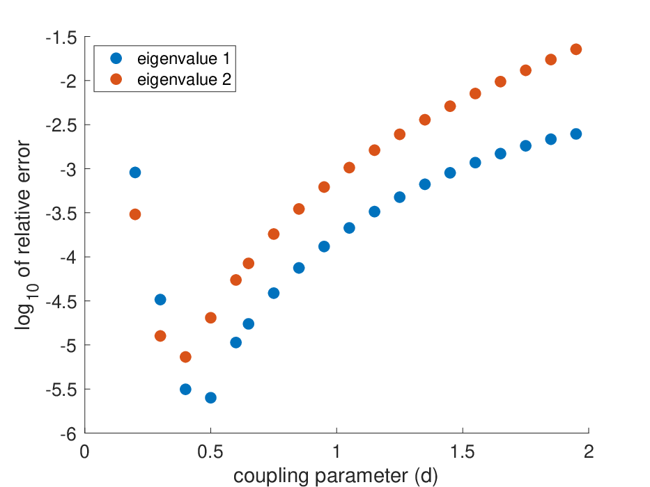
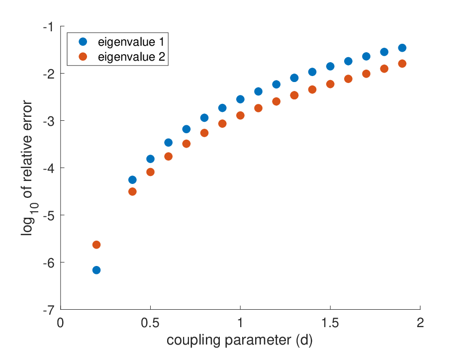
First, we consider the case of equal pulse distances. We use the expressions from Corollary 1 to compute the leading order term for the interaction eigenvalues, and we compare this to the results from Matlab’s eig function. In Fig. 3 we fix the inter-pulse distances and plot the log of the relative error of the eigenvalues versus the coupling parameter dd. For intermediate values of dd, the relative error is less than 10−310^{-3}. Since the results of Theorem Theorem 2 are not uniform in dd, i.e. they hold for sufficiently large NN once dd and ω\omega are chosen, we do not expect to have a nice relationship between the error and dd. This is furthermore complicated by the fact that additional sources of error arise from numerically approximating bib_{i} and MM. In principle, though, the method (and the asymptotic prediction) yields satisfactory results except for the vicinity of the anti-continuum limit (where the notion of the single pulse is highly discrete) and the near-continuum limit (where the role of discreteness is too weak). It is interesting to point out that at a “middle ground” between these two limits, namely around d=0.5d=0.5, we observe the optimal performance of the theoretical prediction.
Refer to caption
Refer to caption
Figure 3: Log of relative error of eigenvalues vs. coupling parameter dd for double (in phase) pulse +⁣+++ (N1=10N_{1}=10) and triple (out-of-phase) pulse +−++-+ (OPENN1=N2=8)N_{1}=N_{2}=8). ω=2\omega=2 in both cases.

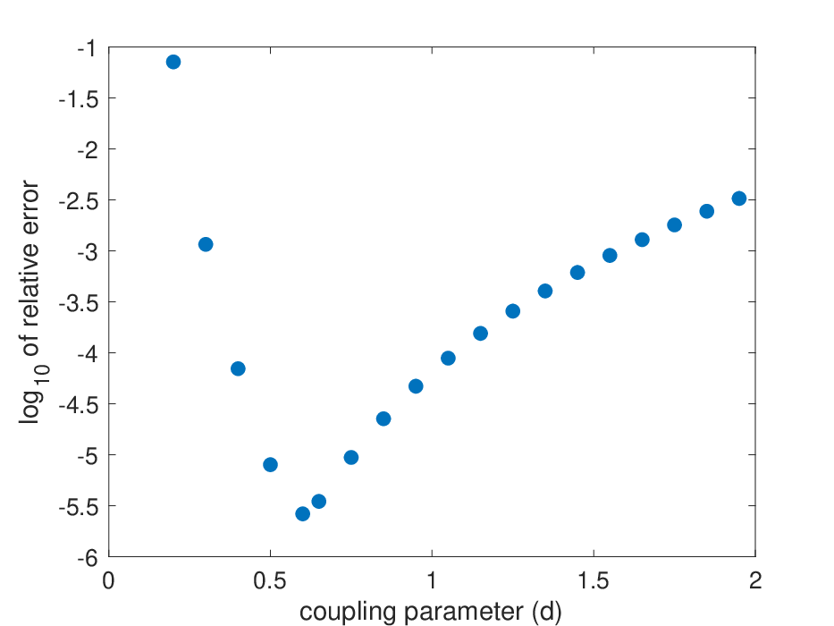
We can also do this for triple pulses with unequal pulse distances. In this case, we use Corollary 2 to compute the eigenvalues to leading order. Fig. 4 shows the log of the relative error of the eigenvalues versus the coupling parameter dd. For intermediate values of dd, the relative error is again less than 10−310^{-3}. Once again this validates the relevance of the method especially so for the case of intermediate ranges of the coupling parameter dd.

Refer to caption
Figure 4: Log of relative error of eigenvalues vs. coupling parameter dd for triple in-phase pulse ++++++ with unequal pulse distances (N1=8,N2=6N_{1}=8,N_{2}=6), ω=2\omega=2.

5 Conclusions & future challenges

In this paper we used Lin’s method to construct multi-pulses in discrete systems and to find the small eigenvalues resulting from interaction between neighboring pulses in these structures. In doing so, we are able to extend known results about DNLS to parameter regimes which are further from the anti-continuum limit. In essence, we replace the requirement that the coupling parameter dd be small by the condition that the pulses are well separated. This method also allows us to estimate these interaction eigenvalues to a good degree of accuracy for intermediate values of dd.

The theoretical results we obtained will apply to many other Hamiltonian systems, as long as the coupling by nodes is via the discrete second order centered difference operator Δ2\Delta_{2}. Since these restrictions were motivated partly by mathematical convenience, future work could extend these results to a broader class of Hamiltonian systems. Indeed, there exist numerous examples worth considering ranging from simpler ones such as discrete multiple-kink states in the discrete sine-Gordon equation [24], to settings of first order PDE discretizations related, e.g., to the Burgers model [28] or even discretizations of third order models such as the Korteweg-de Vries equation [20].

Another direction for future work is characterizing the family of multi-pulse solutions which arises as the coupling parameter dd is varied. Recent work [6] has investigated stationary, spatially localized patterns in lattice dynamical systems which change as a parameter is varied; the coupling parameter in this case is fixed. In some cases, these patterns exist along a closed bifurcation curves known as an isola. Numerical continuation with AUTO in the coupling parameter dd suggests that multi-pulse solutions in DNLS exist on an isola. The parameter dd varies over a bounded interval which includes the origin, thus the isola contains solutions to both the focusing and defocusing equation.

A final direction for future works would concern the consideration of higher dimensional settings. Here, the interaction between pulses would involve the geometric nature of the configuration they form and the “line of sight” between them. The latter is expected (from the limited observations that there exist [14]) to determine the nature of the interaction eigenvalues. Here, however, the scenarios can also be fundamentally richer as coherent states involving topological charge/vorticity may come into play [17]. In the latter case, it is less straightforward to identify what the conclusions may be and considering such more complex configurations (given also their experimental observation [19, 8]) may be of particular interest.

6 Proof of existence theorems

In this section, we will prove Theorem 1 and Theorem 3. Since the proofs are very similar, we will prove Theorem 1 then state what modifications are necessary for the proof of Theorem 3. Throughout this section, we will assume 1, 2, and 3. We begin with setting up the exponential dichotomy necessary for the proof. The technique of the proof is very similar to that in [26].

6.1 Discrete exponential dichotomy

First, we define the discrete evolution operator for linear difference equations.

Lemma 1 (Discrete Evolution Operator).

Consider the difference equation together with its adjoint

V⁡(n+1)\displaystyle V(n+1) =A⁡(n)​V​(n)\displaystyle=A(n)V(n) (56)
Z⁡(n+1)\displaystyle Z(n+1) =[A​(n)−1]∗​Z​(n),\displaystyle=[A(n)^{-1}]^{*}Z(n), (57)

where n∈ℤn\in{\mathbb{Z}}, V⁡(n)∈RdV(n)\in R^{d}, and the matrix A⁡(n)A(n) is invertible for all nn. Define the discrete evolution operator by

Φ⁡(m,n)={Im=nA⁡(m−1)​…​A​(n+1)​A​(n)m>nA−1​(m)​…​A−1​(n−2)​A−1​(n−1)m<n.\Phi(m,n)=\begin{cases}I&m=n\\ A(m-1)\dots A(n+1)A(n)&m>n\\ A^{-1}(m)\dots A^{-1}(n-2)A^{-1}(n-1)&m<n\end{cases}\>. (58)
  1. (i)

    The evolution operators Φ\Phi of Eq. 56 and Ψ\Psi of Eq. 57 are related by

    Ψ⁡(m,n)=Φ​(n,m)∗.\Psi(m,n)=\Phi(n,m)^{*}. (59)
  2. (ii)

    If V⁡(n)V(n) is a solution to Eq. 56 and Z⁡(n)Z(n) is a solution to Eq. 57, then the inner product ⟨V⁡(n),Z⁡(n)⟩\langle V(n),Z(n)\rangle is constant in nn.

Proof.

For (i), the result holds trivially for m=nm=n. For, m<nm<n we have

Ψ⁡(m,n)\displaystyle\Psi(m,n) =A​(m)∗​…​A​(n−2)∗​A​(n−1)∗\displaystyle=A(m)^{*}\dots A(n-2)^{*}A(n-1)^{*}
=[A⁡(n−1)​A​(n−2)​…​A​(m)]∗\displaystyle=[A(n-1)A(n-2)\dots A(m)]^{*}
=Φ​(n,m)∗.\displaystyle=\Phi(n,m)^{*}.

The case for m>nm>n is similar.

For (ii), we have

⟨V⁡(n+1),Z⁡(n+1)⟩\displaystyle\langle V(n+1),Z(n+1)\rangle =⟨A⁡(n)​V​(n),[A​(n)−1]∗​Z​(n)⟩\displaystyle=\langle A(n)V(n),[A(n)^{-1}]^{*}Z(n)\rangle
=⟨A​(n)−1​A​(n)​V​(n),Z⁡(n)⟩\displaystyle=\langle A(n)^{-1}A(n)V(n),Z(n)\rangle
=⟨V⁡(n),Z⁡(n)⟩.\displaystyle=\langle V(n),Z(n)\rangle.

∎

Next, we give a criterion for an exponential dichotomy.

Lemma 2 (Exponential Dichotomy).

Consider the difference equation

V⁡(n+1)=A⁡(n)​V​(n).V(n+1)=A(n)V(n). (60)

Suppose there exists a constant r>1r>1 and a constant coefficient matrix AA such that

|A⁡(n)−A|≤C​r|n||A(n)-A|\leq Cr^{|n|} (61)

and |λ|≥r|\lambda|\geq r or |λ|≤1/r|\lambda|\leq 1/r for all eigenvalues λ\lambda of AA. Then Eq. 60 has exponential dichotomies on Z±Z^{\pm}. Specifically, there exist projections P±sP_{\pm}^{s} and P±uP_{\pm}^{u} defined on ℤ±{\mathbb{Z}}^{\pm} such that the following are true.

  1. (i)

    Let Φ⁡(m,n)\Phi(m,n) be the evolution operator for Eq. 60. Then

    P±s/u​(m)​Φ​(m,n)=Φ⁡(m,n)​P±s/u​(n).P_{\pm}^{s/u}(m)\Phi(m,n)=\Phi(m,n)P_{\pm}^{s/u}(n). (62)
  2. (ii)

    Let Φ±s/u​(m,n)=Φ⁡(m,n)​P±s/u​(n)\Phi_{\pm}^{s/u}(m,n)=\Phi(m,n)P_{\pm}^{s/u}(n) for m,n≥0m,n\geq 0 and m,n≤0m,n\leq 0 (respectively). Then we have the estimates

    |Φ+s​(m,n)|≤C​rm−n\displaystyle|\Phi_{+}^{s}(m,n)|\leq Cr^{m-n} 0≤n≤m\displaystyle 0\leq n\leq m
    |Φ+u​(m,n)|≤C​rn−m\displaystyle|\Phi_{+}^{u}(m,n)|\leq Cr^{n-m} 0≤m≤n\displaystyle 0\leq m\leq n
    |Φ−s​(m,n)|≤C​rm−n\displaystyle|\Phi_{-}^{s}(m,n)|\leq Cr^{m-n} n≤m≤0\displaystyle n\leq m\leq 0
    |Φ−u​(m,n)|≤C​rn−m\displaystyle|\Phi_{-}^{u}(m,n)|\leq Cr^{n-m} m≤n≤0,\displaystyle m\leq n\leq 0\>,

    where the evolution operator Φ⁡(m,n)\Phi(m,n) is defined in Lemma 1.

  3. (iii)

    Let Es/uE^{s/u} be the stable and unstable eigenspaces of AA, and let Qs/uQ^{s/u} the corresponding eigenprojections. Then we have

    dimran⁡P±s​(n)\displaystyle\dim\ran P_{\pm}^{s}(n) =dimEs\displaystyle=\dim E^{s}
    dimran⁡P±u​(n)\displaystyle\dim\ran P_{\pm}^{u}(n) =dimEu\displaystyle=\dim E^{u}

    and the exponential decay rates

    |P±s/u​(n)−Qs/u|≤C​r|n|.\displaystyle|P_{\pm}^{s/u}(n)-Q^{s/u}|\leq Cr^{|n|}. (63)
Proof.

We will consider the problem on ℤ+{\mathbb{Z}}^{+}. Since AA is constant coefficient and hyperbolic, the difference equation W⁡(n+1)=A​W​(n)W(n+1)=AW(n) has an exponential dichotomy on ℝ+{\mathbb{R}}^{+}. All the results except for Eq. 63 follow directly from [2, Proposition 2.5]. Equation Eq. 63 follows from using the estimate Eq. 61 in the proof of [2, Proposition 2.5]. ∎

The last thing we will need is a version of the variation of constants formula for the discrete setting.

Lemma 3 (Discrete variation of constants).

The solution V⁡(n)V(n) to the initial value problem

V⁡(n+1)\displaystyle V(n+1) =A⁡(n)​V​(n)+G⁡(V⁡(n),n)\displaystyle=A(n)V(n)+G(V(n),n)
V⁡(n0)\displaystyle V(n_{0}) =Vn0\displaystyle=V_{n_{0}}

can be written in summation form as

V⁡(n)={Vn0n=n0OPENΦ⁡(n,n0)​Vn0+∑j=n0n−1Φ⁡(n,j+1)​G​(V⁡(j),j))n>n0OPENΦ⁡(n,n0)​Vn0−∑j=nn0−1Φ⁡(n,j+1)​G​(V⁡(j),j))n<n0.V(n)=\begin{cases}V_{n_{0}}&n=n_{0}\\ \Phi(n,n_{0})V_{n_{0}}+\sum_{j=n_{0}}^{n-1}\Phi(n,j+1)G(V(j),j))&n>n_{0}\\ \Phi(n,n_{0})V_{n_{0}}-\sum_{j=n}^{n_{0}-1}\Phi(n,j+1)G(V(j),j))&n<n_{0}\end{cases}\>. (64)
Proof.

For n=n0+1n=n_{0}+1,

V⁡(n0+1)=A⁡(n0)​V​(n0)+G⁡(V⁡(n0),n0)=Φ⁡(n0+1,n0)​V​(n0)+Φ⁡(n0,n0)​G​(V⁡(n0),n0).V(n_{0}+1)=A(n_{0})V(n_{0})+G(V(n_{0}),n_{0})=\Phi(n_{0}+1,n_{0})V(n_{0})+\Phi(n_{0},n_{0})G(V(n_{0}),n_{0}).

Iterate this to get the result for n>n0n>n_{0}. The case for n<n0n<n_{0} is similar. ∎

6.2 Fixed point formulation

To find a solution to the system of equations Eq. 38, we will rewrite the system as a fixed point problem. First, we expand FF in a Taylor series about T⁡(θi)​Q​(n)T(\theta_{i})Q(n) to get

F⁡(Ui±​(n))\displaystyle F(U_{i}^{\pm}(n)) =F⁡(T⁡(θi)​Q​(n)+Q~i±​(n))\displaystyle=F(T(\theta_{i})Q(n)+\tilde{Q}_{i}^{\pm}(n))
=F⁡(T⁡(θi)​Q​(n))+D​F​(T⁡(θi)​Q​(n))​Q~i±​(n)+G⁡(Q~i±​(n))\displaystyle=F(T(\theta_{i})Q(n))+DF(T(\theta_{i})Q(n))\tilde{Q}_{i}^{\pm}(n)+G(\tilde{Q}_{i}^{\pm}(n))
OPEN=T⁡(θi)​D​F​(Q⁡(n))​T​(θi)−1​Q​(n))​Q~i±+G⁡(Q~i±​(n)),\displaystyle=T(\theta_{i})DF(Q(n))T(\theta_{i})^{-1}Q(n))\tilde{Q}_{i}^{\pm}+G(\tilde{Q}_{i}^{\pm}(n)),

where G⁡(Q~i±​(n))=𝒪⁡(|Q~i±|2)G(\tilde{Q}_{i}^{\pm}(n))=\mathcal{O}(|\tilde{Q}_{i}^{\pm}|^{2}) with G⁡(0)=0G(0)=0 and D​G​(0)=0DG(0)=0, and we used the symmetry relation Eq. 17 in the last line. Finally, let

di\displaystyle d_{i} =T⁡(θi+1)​Q​(−Ni−)−T⁡(θi)​Q​(Ni+).\displaystyle=T(\theta_{i+1})Q(-N_{i}^{-})-T(\theta_{i})Q(N_{i}^{+}). (65)

Substituting these into Eq. 38, we obtain the following system of equations for the remainder functions Q~i±\tilde{Q}_{i}^{\pm}.

Q~i±​(n+1)\displaystyle\tilde{Q}_{i}^{\pm}(n+1) =T⁡(θ)​D​F​(Q⁡(n))​T​(θ)−1​Q~i±​(n)+G⁡(Q~i±​(n))\displaystyle=T(\theta)DF(Q(n))T(\theta)^{-1}\tilde{Q}_{i}^{\pm}(n)+G(\tilde{Q}_{i}^{\pm}(n)) (66)
Q~i+​(Ni+)−Wi+1−​(−Ni−)\displaystyle\tilde{Q}_{i}^{+}(N_{i}^{+})-W_{i+1}^{-}(-N_{i}^{-}) =di\displaystyle=d_{i} (67)
Q~i+​(0)−Q~i−​(0)\displaystyle\tilde{Q}_{i}^{+}(0)-\tilde{Q}_{i}^{-}(0) =0.\displaystyle=0. (68)

Next, we look at the variational and adjoint variational equations associated with Eq. 22, which are

V⁡(n+1)\displaystyle V(n+1) =D​F​(Q⁡(n))​V​(n)\displaystyle=DF(Q(n))V(n) (69)
Z⁡(n+1)\displaystyle Z(n+1) =[D​F​(Q⁡(n))∗]−1​Z​(n).\displaystyle=[DF(Q(n))^{*}]^{-1}Z(n). (70)

The variational equation Eq. 69 has a bounded solution T′​(0)​Q​(n)T^{\prime}(0)Q(n), thus we can decompose the tangent spaces to Ws​(0)W^{s}(0) and Wu​(0)W^{u}(0) at Q⁡(0)Q(0) as

TQ⁡(0)​Wu​(0)\displaystyle T_{Q(0)}W^{u}(0) =Y−⊕ℝ​T′​(0)​Q​(0)\displaystyle=Y^{-}\oplus{\mathbb{R}}T^{\prime}(0)Q(0)
TQ⁡(0)​Ws​(0)\displaystyle T_{Q(0)}W^{s}(0) =Y+⊕ℝ​T′​(0)​Q​(0).\displaystyle=Y^{+}\oplus{\mathbb{R}}T^{\prime}(0)Q(0).

The adjoint variational equation also has a unique bounded solution Z1​(n)Z_{1}(n) given by Eq. 35. By Lemma 1, Z1​(0)⟂T′​(0)​Q​(0)⊕Y−⊕Y+Z_{1}(0)\perp T^{\prime}(0)Q(0)\oplus Y^{-}\oplus Y^{+}, thus we can decompose ℝd{\mathbb{R}}^{d} as

ℝd=ℝ​T′​(0)​Q​(0)⊕Y+⊕Y−⊕ℝ​Z1​(0).{\mathbb{R}}^{d}={\mathbb{R}}T^{\prime}(0)Q(0)\oplus Y^{+}\oplus Y^{-}\oplus{\mathbb{R}}Z_{1}(0). (71)

Since T⁡(θ)T(\theta) is unitary, we also have the decomposition

ℝd=ℝ​T​(θi)​T′​(0)​Q​(0)⊕T⁡(θi)​Y+⊕T⁡(θi)​Y−⊕ℝ​T​(θi)​Z1​(0).{\mathbb{R}}^{d}={\mathbb{R}}T(\theta_{i})T^{\prime}(0)Q(0)\oplus T(\theta_{i})Y^{+}\oplus T(\theta_{i})Y^{-}\oplus{\mathbb{R}}T(\theta_{i})Z_{1}(0). (72)

Finally, since perturbations in the direction of T⁡(θi)​T′​(0)​Q​(0)T(\theta_{i})T^{\prime}(0)Q(0) are handled by the symmetry parameter θi\theta_{i}, we may without loss of generality choose Q~i±\tilde{Q}_{i}^{\pm} so that

Q~i±​(0)∈T⁡(θi)​Y+⊕T⁡(θi)​Y−⊕ℝ​T​(θi)​Z1​(0).\tilde{Q}_{i}^{\pm}(0)\in T(\theta_{i})Y^{+}\oplus T(\theta_{i})Y^{-}\oplus{\mathbb{R}}T(\theta_{i})Z_{1}(0). (73)

Let Φ⁡(m,n,θ)\Phi(m,n;\theta) be the evolution operator for

V⁡(n+1,θ)=T⁡(θ)​D​F​(Q⁡(n))​T​(θ)−1​V​(n,θ).V(n+1;\theta)=T(\theta)DF(Q(n))T(\theta)^{-1}V(n;\theta). (74)

We note that since T′​(0)T^{\prime}(0) commutes with T⁡(θ)T(\theta), T′​(0)​Q​(n)T^{\prime}(0)Q(n) is a solution to Eq. 74. Using Eq. 17, the evolution operators are related to those for θ=0\theta=0 by

Φ⁡(m,n,θ)=T⁡(θ)​Φ​(m,n,0)​T​(θ)−1.\Phi(m,n;\theta)=T(\theta)\Phi(m,n;0)T(\theta)^{-1}. (75)

Since T⁡(θ)​D​F​(Q⁡(n))​T​(θ)−1T(\theta)DF(Q(n))T(\theta)^{-1} decays exponentially to T⁡(θ)​D​F​(0)​T​(θ)−1T(\theta)DF(0)T(\theta)^{-1} and D​F​(0)DF(0) is hyperbolic, equation Eq. 74 has exponential dichotomies on ℤ+{\mathbb{Z}}^{+} and ℤ−{\mathbb{Z}}^{-} by Lemma 2, and we note that the estimates from Lemma 2 do not depend on θ\theta. Let Ps/u±​(m,θ)P_{s/u}^{\pm}(m;\theta) and Φs/u±​(m,n,θ)\Phi_{s/u}^{\pm}(m,n;\theta) be the projections and evolutions for this exponential dichotomy on ℤ±{\mathbb{Z}}^{\pm}. The projections Ps/u±​(m,θ)P_{s/u}^{\pm}(m;\theta) are related to those for θ=0\theta=0 by

Ps/u±​(m,θ)=T⁡(θ)​Ps/u±​(m,0)​T​(θ)−1P_{s/u}^{\pm}(m;\theta)=T(\theta)P_{s/u}^{\pm}(m;0)T(\theta)^{-1}

Finally, let Es​(θ)E^{s}(\theta) and Eu​(θ)E^{u}(\theta) be the stable and unstable eigenspaces of T⁡(θ)​DU​F​(0)​T​(θ)−1T(\theta)D_{U}F(0)T(\theta)^{-1}, and let P0s​(θ)P_{0}^{s}(\theta) and P0u​(θ)P_{0}^{u}(\theta) be the corresponding eigenprojections.

Next, as in [26] and [18], we write equation Eq. 66 in fixed-point form using the discrete variation of constants formula Eq. 64 together with projections on the stable and unstable subspaces of the exponential dichotomy.

Q~i−​(n)\displaystyle\tilde{Q}_{i}^{-}(n) =Φs−​(n,−Ni−1−,θi)​ai−1−+Φu−​(n,0,θi)​bi−\displaystyle=\Phi_{s}^{-}(n,-N_{i-1}^{-};\theta_{i})a_{i-1}^{-}+\Phi_{u}^{-}(n,0;\theta_{i})b_{i}^{-} (76)
+∑j=−Ni−1−n−1Φs−(n,j+1;θi)Gi−(Q~i−(j))−∑j=n−1Φu−(n,j+1;θi)Gi−(Q~i−(j))\displaystyle+\sum_{j=-N_{i-1}^{-}}^{n-1}\Phi_{s}^{-}(n,j+1;\theta_{i})G_{i}^{-}(\tilde{Q}_{i}^{-}(j))-\sum_{j=n}^{-1}\Phi_{u}^{-}(n,j+1;\theta_{i})G_{i}^{-}(\tilde{Q}_{i}^{-}(j))
Q~i+​(n)\displaystyle\tilde{Q}_{i}^{+}(n) =Φu+​(n,Ni+,θi)​ai++Φs+​(n,0,θi)​bi+\displaystyle=\Phi_{u}^{+}(n,N_{i}^{+};\theta_{i})a_{i}^{+}+\Phi_{s}^{+}(n,0;\theta_{i})b_{i}^{+}
+∑j=0n−1Φs+(n,j+1;θi)Gi+(Q~i+(j))−∑j=nNi+−1Φu+(n,j+1;θi)Gi+(Q~i+(j)),\displaystyle+\sum_{j=0}^{n-1}\Phi_{s}^{+}(n,j+1;\theta_{i})G_{i}^{+}(\tilde{Q}_{i}^{+}(j))-\sum_{j=n}^{N_{i}^{+}-1}\Phi_{u}^{+}(n,j+1;\theta_{i})G_{i}^{+}(\tilde{Q}_{i}^{+}(j)),

where Q~i−​(n)∈ℓ∞​([−Ni−1−,0])\tilde{Q}_{i}^{-}(n)\in\ell^{\infty}([-N_{i-1}^{-},0]), Q~i+​(n)∈ℓ∞​([0,Ni+])\tilde{Q}_{i}^{+}(n)\in\ell^{\infty}([0,N_{i}^{+}]), and the sums are defined to be 00 if the upper index is smaller than the lower index. For the initial conditions,

  1. 1.

    ai−∈Es​(θi)a_{i}^{-}\in E^{s}(\theta_{i}), ai+∈Eu​(θi)a_{i}^{+}\in E^{u}(\theta_{i}), and a0−=am+=0a_{0}^{-}=a_{m}^{+}=0.

  2. 2.

    bi+∈T⁡(θi)​Y+b_{i}^{+}\in T(\theta_{i})Y^{+} and bi−∈T⁡(θi)​Y−b_{i}^{-}\in T(\theta_{i})Y^{-}.

We note that we do not need to include a component in T′​(0)​Q​(0)T^{\prime}(0)Q(0) in bi±b_{i}^{\pm}, since that direction is handled by the symmetry parameter θi\theta_{i}.

Since we wish to construct a homoclinic orbit to the rest state at 0, we take the initial conditions a0−=0a_{0}^{-}=0 and am+=0a_{m}^{+}=0. For these cases, the fixed point equations are given by

W1−​(n)\displaystyle W_{1}^{-}(n) =Φu−​(n,0,θi)​bi−+∑j=−∞n−1Φs−​(n,j+1,θi)​Gi−​(Q~i−​(j))−∑j=n−1Φu−​(n,j+1,θi)​Gi−​(Q~i−​(j))\displaystyle=\Phi_{u}^{-}(n,0;\theta_{i})b_{i}^{-}+\sum_{j=-\infty}^{n-1}\Phi_{s}^{-}(n,j+1;\theta_{i})G_{i}^{-}(\tilde{Q}_{i}^{-}(j))-\sum_{j=n}^{-1}\Phi_{u}^{-}(n,j+1;\theta_{i})G_{i}^{-}(\tilde{Q}_{i}^{-}(j))
Wm+​(n)\displaystyle W_{m}^{+}(n) =Φs+​(n,0,θi)​bi++∑j=0n−1Φs+​(n,j+1,θi)​Gi+​(Q~i+​(j))−∑j=n∞Φu+​(n,j+1,θi)​Gi+​(Q~i+​(j)),\displaystyle=\Phi_{s}^{+}(n,0;\theta_{i})b_{i}^{+}+\sum_{j=0}^{n-1}\Phi_{s}^{+}(n,j+1;\theta_{i})G_{i}^{+}(\tilde{Q}_{i}^{+}(j))-\sum_{j=n}^{\infty}\Phi_{u}^{+}(n,j+1;\theta_{i})G_{i}^{+}(\tilde{Q}_{i}^{+}(j)),

where the infinite sums converge due to the exponential dichotomy.

6.3 Inversion

As in [26], we will solve equations Eq. 66, Eq. 67, and Eq. 68 in stages. In the first lemma of this section, we solve equation Eq. 66 for Q~i±\tilde{Q}_{i}^{\pm}.

Lemma 4.

There exist unique bounded functions Q~i±​(n)\tilde{Q}_{i}^{\pm}(n) such that equation Eq. 66 is satisfied. These solutions depend smoothly on the initial conditions ai±a_{i}^{\pm} and bi±b_{i}\pm, and we have the estimates

‖Q~i−‖\displaystyle\|\tilde{Q}_{i}^{-}\| ≤C⁡(|ai−1−|+|bi−|)\displaystyle\leq C(|a_{i-1}^{-}|+|b_{i}^{-}|) (77)
‖Q~i+‖\displaystyle\|\tilde{Q}_{i}^{+}\| ≤C⁡(|ai+|+|bi+|).\displaystyle\leq C(|a_{i}^{+}|+|b_{i}^{+}|)\>.

For the interior pieces, we have the piecewise estimates

|Q~i−​(n)|\displaystyle|\tilde{Q}_{i}^{-}(n)| ≤C⁡(r−(Ni−1−+n)​|ai−1−|+rn​|bi−|)\displaystyle\leq C(r^{-(N_{i-1}^{-}+n)}|a_{i-1}^{-}|+r^{n}|b_{i}^{-}|) n∈[−Ni−1−,0]\displaystyle n\in[-N_{i-1}^{-},0] (78)
|Q~i+​(n)|\displaystyle|\tilde{Q}_{i}^{+}(n)| ≤C⁡(r−(Ni+−n)​|ai+|+r−n​|bi+|)\displaystyle\leq C(r^{-(N_{i}^{+}-n)}|a_{i}^{+}|+r^{-n}|b_{i}^{+}|) n∈[0,Ni+].\displaystyle n\in[0,N_{i}^{+}]\>.
Proof.

First, we show that the RHS of the fixed point equations Eq. 76 defines a smooth map from ℓ∞\ell^{\infty} (on the appropriate interval) to itself. For the Q~i−\tilde{Q}_{i}^{-}, we have

|Φs−(n,\displaystyle|\Phi_{s}^{-}(n, OPEN−Ni−1−;θi)​ai−1−|+|Φu−​(n,0,θi)​bi−|≤C⁡(|ai−1−|+|bi−|)\displaystyle-N_{i-1}^{-};\theta_{i})a_{i-1}^{-}|+|\Phi_{u}^{-}(n,0;\theta_{i})b_{i}^{-}|\leq C(|a_{i-1}^{-}|+|b_{i}^{-}|) (79)

and

|∑j=−Ni−1−n−1Φs−​(n,j+1,θi)​Gi−​(Q~i−​(j))|+|∑j=n−1Φu−​(n,j+1,θi)​Gi−​(Q~i−​(j))|≤C​‖Q~i−‖ℓ∞​([−Ni−1,0])2,\displaystyle\left|\sum_{j=-N_{i-1}^{-}}^{n-1}\Phi_{s}^{-}(n,j+1;\theta_{i})G_{i}^{-}(\tilde{Q}_{i}^{-}(j))\right|+\left|\sum_{j=n}^{-1}\Phi_{u}^{-}(n,j+1;\theta_{i})G_{i}^{-}(\tilde{Q}_{i}^{-}(j))\right|\leq C\|\tilde{Q}_{i}^{-}\|_{\ell^{\infty}([-N_{i-1},0])}^{2}\>,

both of which are independent of nn. Define the map Ki−:ℓ∞​([−Ni−1,0])×Es×Y−→ℓ∞​([−Ni−1,0])K_{i}^{-}:\ell^{\infty}([-N_{i-1},0])\times E^{s}\times Y^{-}\rightarrow\ell^{\infty}([-N_{i-1},0]) by

Ki−​(Q~i−​(n)CLOSE,\displaystyle K_{i}^{-}(\tilde{Q}_{i}^{-}(n), OPENai−1−,bi−)=Q~i−​(n)−Φs−​(n,−Ni−1−,θi)​ai−1−−Φu−​(n,0,θi)​bi−\displaystyle a_{i-1}^{-},b_{i}^{-})=\tilde{Q}_{i}^{-}(n)-\Phi_{s}^{-}(n,-N_{i-1}^{-};\theta_{i})a_{i-1}^{-}-\Phi_{u}^{-}(n,0;\theta_{i})b_{i}^{-} (80)
−∑j=−Ni−1−n−1Φs−(n,j+1;θi)Gi−(Q~i−(j))+∑j=n−1Φu−(n,j+1;θi)Gi−(Q~i−(j)).\displaystyle-\sum_{j=-N_{i-1}^{-}}^{n-1}\Phi_{s}^{-}(n,j+1;\theta_{i})G_{i}^{-}(\tilde{Q}_{i}^{-}(j))+\sum_{j=n}^{-1}\Phi_{u}^{-}(n,j+1;\theta_{i})G_{i}^{-}(\tilde{Q}_{i}^{-}(j)).

Since 0 is an equilibrium, K⁡(0,0,0)=0K(0,0,0)=0. It is straightforward to show that the Fréchet derivative of Ki−K_{i}^{-} with respect to Q~i−\tilde{Q}_{i}^{-} at (Q~i−​(n),ai−1−,bi−)=(0,0,0)(\tilde{Q}_{i}^{-}(n),a_{i-1}^{-},b_{i}^{-})=(0,0,0) is a Banach space isomorphism on l∞​([−Ni−1,0])l^{\infty}([-N_{i-1},0]). Thus we can solve for Q~i−​(x)\tilde{Q}_{i}^{-}(x) in terms of (ai−1−,bi−)(a_{i-1}^{-},b_{i}^{-}) using the IFT. This dependence is smooth, since the map Ki−K_{i}^{-} is smooth. The estimate Eq. 77 on Q~i−\tilde{Q}_{i}^{-} comes from Eq. 79, since the terms in Eq. 80 involving sums are quadratic in Q~i±\tilde{Q}_{i}^{\pm}. The case for Q~i+\tilde{Q}_{i}^{+} is similar. It is not hard to obtain the piecewise estimates Eq. 78 for the interior pieces. ∎

Next, we use the center matching conditions at Ni±N_{i}^{\pm} to solve equation Eq. 67. This will give us the initial conditions ai±a_{i}^{\pm}.

Lemma 5.

For i=1,…​m−1i=1,\dots m-1 there is a unique pair of initial conditions (ai+,ai−)∈Eu​(θi)×Es​(θi)(a_{i}^{+},a_{i}^{-})\in E^{u}(\theta_{i})\times E^{s}(\theta_{i}) such that the matching conditions Eq. 67 are satisfied. (ai+,ai−)(a_{i}^{+},a_{i}^{-}) depends smoothly on (bi+,bi+1−)(b_{i}^{+},b_{i+1}^{-}), and we have the following expressions for ai−a_{i}^{-} and ai+a_{i}^{+}.

ai+\displaystyle a_{i}^{+} =P0u​(θi)​di+a~i+\displaystyle=P_{0}^{u}(\theta_{i})d_{i}+\tilde{a}_{i}^{+} (81)
ai−\displaystyle a_{i}^{-} =−P0s​(θi)​di+a~i−,\displaystyle=-P_{0}^{s}(\theta_{i})d_{i}+\tilde{a}_{i}^{-},

where

a~i±=𝒪⁡(r−N​(|bi+|+|bi+1−|)+|bi+|2+|bi+1−|2).\tilde{a}_{i}^{\pm}=\mathcal{O}(r^{-N}(|b_{i}^{+}|+|b_{i+1}^{-}|)+|b_{i}^{+}|^{2}+|b_{i+1}^{-}|^{2}). (82)

In terms of Q⁡(±Ni±)Q(\pm N_{i}^{\pm}), we can write Eq. 81 as

ai−\displaystyle a_{i}^{-} =T⁡(θi)​Q​(Ni+)+a~i−+𝒪⁡(r−2​N)\displaystyle=T(\theta_{i})Q(N_{i}^{+})+\tilde{a}_{i}^{-}+\mathcal{O}(r^{-2N}) (83)
ai+\displaystyle a_{i}^{+} =T⁡(θi+1)​Q​(−Ni−)+a~i++𝒪⁡(r−2​N).\displaystyle=T(\theta_{i+1})Q(-N_{i}^{-})+\tilde{a}_{i}^{+}+\mathcal{O}(r^{-2N}).
Proof.

Evaluating the fixed point equations Eq. 76 at ±Ni±\pm N_{i}^{\pm} and subtracting, solving equation Eq. 67 is equivalent to solving Ki​(ai+,ai−,bi+,bi+1−)=0K_{i}(a_{i}^{+},a_{i}^{-},b_{i}^{+},b_{i+1}^{-})=0, where Ki:Es×Eu×Y+×Y−→ℝdK_{i}:E^{s}\times E^{u}\times Y^{+}\times Y^{-}\rightarrow{\mathbb{R}}^{d} is defined by

Ki​(ai+CLOSE,\displaystyle K_{i}(a_{i}^{+}, OPENai−,bi+,bi+1−)\displaystyle a_{i}^{-},b_{i}^{+},b_{i+1}^{-})
=ai+−ai−−di+(Pu+​(Ni+,θi)−P0u)​ai+−(Ps−​(−Ni−,θi+1)−P0s)​ai−\displaystyle=a_{i}^{+}-a_{i}^{-}-d_{i}+(P_{u}^{+}(N_{i}^{+};\theta_{i})-P_{0}^{u})a_{i}^{+}-(P_{s}^{-}(-N_{i}^{-};\theta_{i+1})-P_{0}^{s})a_{i}^{-}
+Φs+​(Ni+,0,θi)​bi+−Φu−​(−Ni−,0,θi+1)​bi+1−\displaystyle+\Phi_{s}^{+}(N_{i}^{+},0;\theta_{i})b_{i}^{+}-\Phi_{u}^{-}(-N_{i}^{-},0;\theta_{i+1})b_{i+1}^{-}
+∑j=0Ni+−1Φs+(Ni+,j+1;θi)Gi+(Q~i+(j;ai+,bi+))\displaystyle+\sum_{j=0}^{N_{i}^{+}-1}\Phi_{s}^{+}(N_{i}^{+},j+1;\theta_{i})G_{i}^{+}(\tilde{Q}_{i}^{+}(j;a_{i}^{+},b_{i}^{+}))
+∑j=−Ni−−1Φu−(−Ni−,j+1;θi+1)Gi−(Q~i+1−(j;ai−,bi+1−)),\displaystyle+\sum_{j=-N_{i}^{-}}^{-1}\Phi_{u}^{-}(-N_{i}^{-},j+1;\theta_{i+1})G_{i}^{-}(\tilde{Q}_{i+1}^{-}(j;a_{i}^{-},b_{i+1}^{-})),

and we substituted Wi+1−​(n,ai−,bi+1−)W_{i+1}^{-}(n;a_{i}^{-},b_{i+1}^{-}) and Q~i+​(n,ai+,bi+)\tilde{Q}_{i}^{+}(n;a_{i}^{+},b_{i}^{+}) from Lemma 4. Next, we note that Ki​(0,0,0,0)=0K_{i}(0,0,0,0)=0 and that

∂∂ai−​Ki​(0,0,0,0)\displaystyle\frac{\partial}{\partial a_{i}^{-}}K_{i}(0,0,0,0) =−1+𝒪⁡(r−Ni−)\displaystyle=-1+\mathcal{O}(r^{-N_{i}^{-}})
∂∂ai+​Ki​(0,0,0,0)\displaystyle\frac{\partial}{\partial a_{i}^{+}}K_{i}(0,0,0,0) =1+𝒪⁡(r−Ni+),\displaystyle=1+\mathcal{O}(r^{-N_{i}^{+}}),

since the derivatives of the terms in KiK_{i} involving sums will be 0 since Gi±G_{i}^{\pm} is quadratic in Q~i±\tilde{Q}_{i}^{\pm}, thus quadratic order in ai±a_{i}^{\pm} by Lemma 4. For sufficiently large NN, Dai±​K​(0,0,0,0,0)D_{a_{i}^{\pm}}K(0,0,0,0,0) is invertible in a neighborhood of (0,0,0,0,0)(0,0,0,0,0). Thus, since (ai+,ai−)∈Es​(θi)⊕Eu​(θi)=ℝd(a_{i}^{+},a_{i}^{-})\in E^{s}(\theta_{i})\oplus E^{u}(\theta_{i})={\mathbb{R}}^{d}, we can use the IFT to solve for ai±a_{i}^{\pm} in terms of (bi+CLOSE(b_{i}^{+}, OPENbi+1−)b_{i+1}^{-}) for (bi+,bi+1−)(b_{i}^{+},b_{i+1}^{-}) sufficiently small.

To get the estimates on and expressions for ai±a_{i}^{\pm}, we project Ki​(ai+,ai−,bi+,bi+1−)=0K_{i}(a_{i}^{+},a_{i}^{-},b_{i}^{+},b_{i+1}^{-})=0 onto Es​(θi)E^{s}(\theta_{i}) and Eu​(θi)E^{u}(\theta_{i}) in turn to get

ai+\displaystyle a_{i}^{+} =P0u​(θi)​di+𝒪⁡(r−N​(|bi+|+|bi+1−|)+|bi+|2+|bi+1−|2)\displaystyle=P_{0}^{u}(\theta_{i})d_{i}+\mathcal{O}(r^{-N}(|b_{i}^{+}|+|b_{i+1}^{-}|)+|b_{i}^{+}|^{2}+|b_{i+1}^{-}|^{2})
ai−\displaystyle a_{i}^{-} =−P0s​(θi)​di+𝒪⁡(r−N​(|bi+|+|bi+1−|)+|bi+|2+|bi+1−|2),\displaystyle=-P_{0}^{s}(\theta_{i})d_{i}+\mathcal{O}(r^{-N}(|b_{i}^{+}|+|b_{i+1}^{-}|)+|b_{i}^{+}|^{2}+|b_{i+1}^{-}|^{2}),

which we can write in the form Eq. 81 with estimates Eq. 82.

To write these in terms of Q⁡(±Ni±)Q(\pm N_{i}^{\pm}), we note that

P0s​(θi)​T​(θi)​Q​(Ni+)\displaystyle P_{0}^{s}(\theta_{i})T(\theta_{i})Q(N_{i}^{+}) =(P0s​(θi)−Ps+​(Ni+,θi))​T​(θi)​Q​(Ni+)+Ps+​(Ni+,θi)​T​(θi)​Q​(Ni+)\displaystyle=(P_{0}^{s}(\theta_{i})-P_{s}^{+}(N_{i}^{+};\theta_{i}))T(\theta_{i})Q(N_{i}^{+})+P_{s}^{+}(N_{i}^{+};\theta_{i})T(\theta_{i})Q(N_{i}^{+})
=T⁡(θi)​(P0s​(0)−Ps+​(Ni+,0))​Q​(Ni+)+Ps+​(Ni+,θi)​T​(θi)​Q​(Ni+)\displaystyle=T(\theta_{i})(P_{0}^{s}(0)-P_{s}^{+}(N_{i}^{+};0))Q(N_{i}^{+})+P_{s}^{+}(N_{i}^{+};\theta_{i})T(\theta_{i})Q(N_{i}^{+})
=T⁡(θi)​Q​(Ni+)+𝒪⁡(r−2​N),\displaystyle=T(\theta_{i})Q(N_{i}^{+})+\mathcal{O}(r^{-2N}),

where in the second line we used Eq. 63. Similarly, we can show that

P0s​T​(θi+1)​Q​(−Ni−)\displaystyle P_{0}^{s}T(\theta_{i+1})Q(-N_{i}^{-}) =𝒪⁡(r−2​N).\displaystyle=\mathcal{O}(r^{-2N}).

Substituting these into Eq. 81 we obtain Eq. 83. ∎

It only remains to satisfy Eq. 68, which is the jump condition at 0. We will not in general be able to solve equation Eq. 68. In the next lemma, we will solve for the initial conditions bi±b_{i}^{\pm}. This will give us a unique solution which will generically have mm jumps in the direction of T⁡(θ)​Z1​(0)T(\theta)Z_{1}(0). We will obtain a set of mm jump conditions in the direction of T⁡(θ)​Z1​(0)T(\theta)Z_{1}(0) which will depend on the symmetry parameters θi\theta_{i}. Satisfying the jump conditions, which solves Eq. 68, can be accomplished by adjusting the symmetry parameters.

Recall that for all θ∈ℝ\theta\in{\mathbb{R}} we have the decomposition

ℝd=ℝ​T​(θ)​T′​(0)​Q​(0)⊕T⁡(θ)​Y+⊕T⁡(θ)​Y−⊕ℝ​T​(θ)​Z1​(0).{\mathbb{R}}^{d}={\mathbb{R}}T(\theta)T^{\prime}(0)Q(0)\oplus T(\theta)Y^{+}\oplus T(\theta)Y^{-}\oplus{\mathbb{R}}T(\theta)Z_{1}(0).

Projecting in these directions, we can write Eq. 68 as the system of equations

PT⁡(θi)​T′​(0)​Q​(0)​(Q~i+​(0)−Q~i−​(0))\displaystyle P_{T(\theta_{i})T^{\prime}(0)Q(0)}\left(\tilde{Q}_{i}^{+}(0)-\tilde{Q}_{i}^{-}(0)\right) =0\displaystyle=0 (84)
PT⁡(θi)​Y+⊕T⁡(θi)​Y−​(Q~i+​(0)−Q~i−​(0))\displaystyle P_{T(\theta_{i})Y^{+}\oplus T(\theta_{i})Y^{-}}\left(\tilde{Q}_{i}^{+}(0)-\tilde{Q}_{i}^{-}(0)\right) =0\displaystyle=0 (85)
Pℝ​T​(θi)​Z1​(0)​(Q~i+​(0)−Q~i−​(0))\displaystyle P_{{\mathbb{R}}T(\theta_{i})Z_{1}(0)}\left(\tilde{Q}_{i}^{+}(0)-\tilde{Q}_{i}^{-}(0)\right) =0.\displaystyle=0. (86)

Since Q~i±​(0)∈Y+⊕Y−⊕ℝ​Z1​(0)\tilde{Q}_{i}^{\pm}(0)\in Y^{+}\oplus Y^{-}\oplus{\mathbb{R}}Z_{1}(0), equation Eq. 84 is automatically satisfied. Since bi+∈T⁡(θ)​Y+b_{i}^{+}\in T(\theta)Y^{+} and bi−∈T⁡(θ)​Y−b_{i}^{-}\in T(\theta)Y^{-}, we will be able to satisfy Eq. 85 by solving for the bi±b_{i}^{\pm}, which we do in the following lemma.

Lemma 6.

For i=1,…​mi=1,\dots m there is a unique pair of initial conditions (bi−,bi+)∈T⁡(θi)​Y−×T⁡(θi)​Y+(b_{i}^{-},b_{i}^{+})\in T(\theta_{i})Y^{-}\times T(\theta_{i})Y^{+} such that Eq. 85 is satisfied. We have the uniform bound

b=𝒪⁡(r−2​N).b=\mathcal{O}(r^{-2N}). (87)
Proof.

For convenience, let Xi=T⁡(θi)​Y+⊕T⁡(θi)​Y−X_{i}=T(\theta_{i})Y^{+}\oplus T(\theta_{i})Y^{-}. Evaluating the fixed point equations Eq. 76 at 0, subtracting, and applying the projection PXiP_{X_{i}} to both sides, we have

PXi​(Q~i+​(0)CLOSE\displaystyle P_{X_{i}}(\tilde{Q}_{i}^{+}(0) OPEN−Q~i−​(0))=bi+−bi−+PXi​(Φu+​(0,Ni+,θi)​ai+)−PXi​(Φs−​(0,−Ni−1−,θi)​ai−1−)\displaystyle-\tilde{Q}_{i}^{-}(0))=b_{i}^{+}-b_{i}^{-}+P_{X_{i}}(\Phi_{u}^{+}(0,N_{i}^{+};\theta_{i})a_{i}^{+})-P_{X_{i}}(\Phi_{s}^{-}(0,-N_{i-1}^{-};\theta_{i})a_{i-1}^{-})
−PXi​(∑j=0Ni+−1Φu+​(0,j+1,θi)​Gi+​(Q~i+​(j))−∑j=−Ni−1−−1Φs−​(0,j+1,θi)​Gi−​(Q~i−​(j))).\displaystyle-P_{X_{i}}\left(\sum_{j=0}^{N_{i}^{+}-1}\Phi_{u}^{+}(0,j+1;\theta_{i})G_{i}^{+}(\tilde{Q}_{i}^{+}(j))-\sum_{j=-N_{i-1}^{-}}^{-1}\Phi_{s}^{-}(0,j+1;\theta_{i})G_{i}^{-}(\tilde{Q}_{i}^{-}(j))\right).

Next, substitute Q~i±\tilde{Q}_{i}^{\pm} from Lemma 4 and ai±a_{i}^{\pm} from Lemma 5. Define the spaces

Y\displaystyle Y =⨁i=1m(T⁡(θ)​Y+⊕T⁡(θ)​Y−)=⨁i=1mℝd\displaystyle=\bigoplus_{i=1}^{m}(T(\theta)Y^{+}\oplus T(\theta)Y^{-})=\bigoplus_{i=1}^{m}{\mathbb{R}}^{d} (88)
Z\displaystyle Z =⨁i=1m−1ℝd.\displaystyle=\bigoplus_{i=1}^{m-1}{\mathbb{R}}^{d}. (89)

Let b=(b1+,b1−,…,bm+,bm−)∈Yb=(b_{1}^{+},b_{1}^{-},\dots,b_{m}^{+},b_{m}^{-})\in Y and d=(d1,…,dm−1)∈Zd=(d_{1},\dots,d_{m-1})\in Z. Define the function K:Y×Z→YK:Y\times Z\rightarrow Y component-wise by

Ki​(b,d)\displaystyle K_{i}(b,d) =bi+−bi−+PXi​(Φu+​(0,Ni+,θi)​P0u​di+Φs−​(0,−Ni−1−,θi)​P0s​di−1)\displaystyle=b_{i}^{+}-b_{i}^{-}+P_{X_{i}}\left(\Phi_{u}^{+}(0,N_{i}^{+};\theta_{i})P_{0}^{u}d_{i}+\Phi_{s}^{-}(0,-N_{i-1}^{-};\theta_{i})P_{0}^{s}d_{i-1}\right)
+PXi​(Φu+​(0,Ni+,θi)​a~i+​(bi+,bi+1−)−Φs−​(0,−Ni−1−,θi)​a~i−1−​(bi−1+,bi−))\displaystyle+P_{X_{i}}\left(\Phi_{u}^{+}(0,N_{i}^{+};\theta_{i})\tilde{a}_{i}^{+}(b_{i}^{+},b_{i+1}^{-})-\Phi_{s}^{-}(0,-N_{i-1}^{-};\theta_{i})\tilde{a}_{i-1}^{-}(b_{i-1}^{+},b_{i}^{-})\right)
−PXi∑j=0Ni+−1Φu+(0,j+1;θi)Gi+(Q~i+(j;bi+,bi+1−))\displaystyle-P_{X_{i}}\sum_{j=0}^{N_{i}^{+}-1}\Phi_{u}^{+}(0,j+1;\theta_{i})G_{i}^{+}(\tilde{Q}_{i}^{+}(j;b_{i}^{+},b_{i+1}^{-}))
−PXi∑j=−Ni−1−−1Φs−(0,j+1;θi)Gi−(Q~i−(j;bi−1+,bi−)),\displaystyle-P_{X_{i}}\sum_{j=-N_{i-1}^{-}}^{-1}\Phi_{s}^{-}(0,j+1;\theta_{i})G_{i}^{-}(\tilde{Q}_{i}^{-}(j;b_{i-1}^{+},b_{i}^{-})),

where d0=dm=0d_{0}=d_{m}=0, and we have indicated the dependencies on the bi±b_{i}^{\pm}. Using the estimates from Lemma 4 and Lemma 5, K⁡(0,0)=0K(0,0)=0. For the partial derivatives with respect to bi±b_{i}^{\pm}, we have

∂∂bi+​Ki​(0)\displaystyle\frac{\partial}{\partial b_{i}^{+}}K_{i}(0) =1+𝒪⁡(r−N)\displaystyle=1+\mathcal{O}(r^{-N})
∂∂bi−​Ki​(0)\displaystyle\frac{\partial}{\partial b_{i}^{-}}K_{i}(0) =−1+𝒪⁡(r−N)\displaystyle=-1+\mathcal{O}(r^{-N})
∂∂bi−1+​Ki​(0),∂∂bi+1−​Ki​(0)\displaystyle\frac{\partial}{\partial b_{i-1}^{+}}K_{i}(0),\frac{\partial}{\partial b_{i+1}^{-}}K_{i}(0) =𝒪⁡(r−N).\displaystyle=\mathcal{O}(r^{-N}).

For all other indices,

∂∂bj±​Ki​(0)=0.\frac{\partial}{\partial b_{j}^{\pm}}K_{i}(0)=0.

Thus, for sufficiently large NN, the matrix Db​K​(0,0)D_{b}K(0,0) is invertible. Using the IFT, there exists a unique smooth function b:Z→Yb:Z\rightarrow Y with b⁡(0)=0b(0)=0 such that K⁡(b⁡(d),d)=0K(b(d),d)=0 for dd sufficiently small, which is the case for NN sufficiently large, since d=𝒪⁡(r−N)d=\mathcal{O}(r^{-N}). The bound for bb comes from projecting Ki​(b​(d),d)=0K_{i}(b(d),d)=0 onto T⁡(θ)​Y+T(\theta)Y^{+} and T⁡(θ)​Y−T(\theta)Y^{-} together with the estimate d=𝒪⁡(r−N)d=\mathcal{O}(r^{-N}). ∎

Finally, we will use Eq. 86 to derive the jump conditions in the direction of T⁡(θi)​Z1T(\theta_{i})Z_{1}.

Lemma 7.

The jump conditions in the direction of T⁡(θi)​Z1T(\theta_{i})Z_{1} are given by

ξ1\displaystyle\xi_{1} =⟨T⁡(θ1)​Z1​(N1+),T⁡(θ2)​Q​(−N1−)⟩+R1=0\displaystyle=\langle T(\theta_{1})Z_{1}(N_{1}^{+}),T(\theta_{2})Q(-N_{1}^{-})\rangle+R_{1}=0
ξi\displaystyle\xi_{i} =⟨T⁡(θi)​Z1​(Ni+),T⁡(θi+1)​Q​(−Ni−)⟩\displaystyle=\langle T(\theta_{i})Z_{1}(N_{i}^{+}),T(\theta_{i+1})Q(-N_{i}^{-})\rangle
−⟨T⁡(θi)​Z1​(−Ni−1−),T⁡(θi−1)​Q​(Ni−1+)⟩+Ri=0\displaystyle-\langle T(\theta_{i})Z_{1}(-N_{i-1}^{-}),T(\theta_{i-1})Q(N_{i-1}^{+})\rangle+R_{i}=0 i=2,…,m−1\displaystyle i=2,\dots,m-1
ξm\displaystyle\xi_{m} =−⟨T⁡(θm)​Z1​(−Nm−1−),T⁡(θm−1)​Q​(Nm−1+)⟩+Rm=0,\displaystyle=-\langle T(\theta_{m})Z_{1}(-N_{m-1}^{-}),T(\theta_{m-1})Q(N_{m-1}^{+})\rangle+R_{m}=0,

where the remainder term has bound

|Ri|≤C​r−3​N.|R_{i}|\leq Cr^{-3N}. (90)
Proof.

Evaluating the fixed point equations Eq. 76 at 0 and substituting Eq. 81 from Lemma 4, we get

Q~i+​(0)\displaystyle\tilde{Q}_{i}^{+}(0) −Q~i−​(0)=Φu+​(0,Ni+,θi)​P0u​(θi)​di+Φs−​(0,−Ni−1−,θi)​P0s​(θi−1)​di−1\displaystyle-\tilde{Q}_{i}^{-}(0)=\Phi_{u}^{+}(0,N_{i}^{+};\theta_{i})P_{0}^{u}(\theta_{i})d_{i}+\Phi_{s}^{-}(0,-N_{i-1}^{-};\theta_{i})P_{0}^{s}(\theta_{i-1})d_{i-1}
+bi+−bi−+Φu+​(0,Ni+,θi)​a~i+−Φs−​(0,−Ni−1−,θi)​a~i−1−\displaystyle+b_{i}^{+}-b_{i}^{-}+\Phi_{u}^{+}(0,N_{i}^{+};\theta_{i})\tilde{a}_{i}^{+}-\Phi_{s}^{-}(0,-N_{i-1}^{-};\theta_{i})\tilde{a}_{i-1}^{-}
−∑j=0Ni+−1Φu+(0,j+1;θi)Gi+(Q~i+(j))−∑j=−Ni−1−−1Φs−(0,j+1;θi)Gi−(Q~i−(j)).\displaystyle-\sum_{j=0}^{N_{i}^{+}-1}\Phi_{u}^{+}(0,j+1;\theta_{i})G_{i}^{+}(\tilde{Q}_{i}^{+}(j))-\sum_{j=-N_{i-1}^{-}}^{-1}\Phi_{s}^{-}(0,j+1;\theta_{i})G_{i}^{-}(\tilde{Q}_{i}^{-}(j)).

Next, we project on ℝ​T​(θi)​Z1​(0){\mathbb{R}}T(\theta_{i})Z_{1}(0) by taking the inner product with T⁡(θi)​Z1​(0)T(\theta_{i})Z_{1}(0). Since bi±∈T⁡(θi)​Yi±b_{i}^{\pm}\in T(\theta_{i})Y_{i}^{\pm}, these terms are eliminated by the projection. For the leading order terms in Eq. 86, using equation Eq. 65 and the proof of Lemma 5, we have

⟨T⁡(θi)​Z1​(0),Φu+​(0,Ni+,θi)​P0u​di⟩\displaystyle\langle T(\theta_{i})Z_{1}(0),\Phi_{u}^{+}(0,N_{i}^{+};\theta_{i})P_{0}^{u}d_{i}\rangle =⟨T⁡(θi)​Z1​(Ni+),T⁡(θi+1)​Q​(−Ni−)⟩+𝒪⁡(r−3​N)\displaystyle=\langle T(\theta_{i})Z_{1}(N_{i}^{+}),T(\theta_{i+1})Q(-N_{i}^{-})\rangle+\mathcal{O}(r^{-3N})
⟨T⁡(θi)​Z1​(0),Φs−​(0,−Ni−1−,θi)​P0s​di−1⟩\displaystyle\langle T(\theta_{i})Z_{1}(0),\Phi_{s}^{-}(0,-N_{i-1}^{-};\theta_{i})P_{0}^{s}d_{i-1}\rangle =−⟨T⁡(θi)​Z1​(−Ni−1−),T⁡(θi−1)​Q​(Ni−1+)⟩+𝒪⁡(r−3​N).\displaystyle=-\langle T(\theta_{i})Z_{1}(-N_{i-1}^{-}),T(\theta_{i-1})Q(N_{i-1}^{+})\rangle+\mathcal{O}(r^{-3N}).

For the higher order terms in Eq. 86, we substitute Q~i±\tilde{Q}_{i}^{\pm} from Lemma 4, a~i±\tilde{a}_{i}^{\pm} from Lemma 5, and bi±b_{i}^{\pm} from Lemma 6. This gives us the remainder bound Eq. 90. Since N0−=Nm+=∞N_{0}^{-}=N_{m}^{+}=\infty, one of the two inner product terms vanishes in the jumps ξ1\xi_{1} and ξm\xi_{m}. ∎

6.4 Proof of Theorem 1

The existence statement follows from the jump conditions in Lemma 7. The uniform bound ‖Q~i±‖≤C​r−N\|\tilde{Q}_{i}^{\pm}\|\leq Cr^{-N} in Eq. 40 follows from Lemma 4 together with the estimates on ai±a_{i}^{\pm} and bi±b_{i}^{\pm}. For the second estimate in Eq. 40, recall that in Lemma 5 we solved

Q~i+​(Ni+)−Q~i+1−​(−Ni−)=T⁡(θi+1)​Q​(−Ni−)−T⁡(θi)​Q​(Ni+).\tilde{Q}_{i}^{+}(N_{i}^{+})-\tilde{Q}_{i+1}^{-}(-N_{i}^{-})=T(\theta_{i+1})Q(-N_{i}^{-})-T(\theta_{i})Q(N_{i}^{+}). (91)

Apply the projection P−u​(−Ni−,θi+1)P^{u}_{-}(-N_{i}^{-};\theta_{i+1}), noting that it acts as the identity on T⁡(θi+1)​Q​(−Ni−)T(\theta_{i+1})Q(-N_{i}^{-}). We look at the three remaining terms in Eq. 91 one at a time. For T⁡(θi)​Q​(Ni+)T(\theta_{i})Q(N_{i}^{+}), we follow the proof of Lemma 5 and use the estimate Eq. 63 to get

P−u​(−Ni−,θi+1)​T​(θi)​Q​(Ni+)\displaystyle P^{u}_{-}(-N_{i}^{-};\theta_{i+1})T(\theta_{i})Q(N_{i}^{+}) =𝒪⁡(r−2​N).\displaystyle=\mathcal{O}(r^{-2N}).

For Q~i+​(Ni+)\tilde{Q}_{i}^{+}(N_{i}^{+}), we use the fixed point equations Eq. 76 and the uniform bound on Q~i±\tilde{Q}_{i}^{\pm} from Lemma 4 to get

(I−CLOSE\displaystyle(I- OPENP−u​(−Ni−,θi+1))​Q~i+​(Ni+)=P−s​(−Ni−,θi+1)​Q~i+​(Ni+)=𝒪⁡(r−2​N),\displaystyle P^{u}_{-}(-N_{i}^{-};\theta_{i+1}))\tilde{Q}_{i}^{+}(N_{i}^{+})=P^{s}_{-}(-N_{i}^{-};\theta_{i+1})\tilde{Q}_{i}^{+}(N_{i}^{+})=\mathcal{O}(r^{-2N}),

from which it follows that

P−u​(−Ni−,θi+1)​Q~i+​(Ni+)=Q~i+​(Ni+)+𝒪⁡(r−2​N).P^{u}_{-}(-N_{i}^{-};\theta_{i+1})\tilde{Q}_{i}^{+}(N_{i}^{+})=\tilde{Q}_{i}^{+}(N_{i}^{+})+\mathcal{O}(r^{-2N}).

For Q~i+1−​(−Ni−)\tilde{Q}_{i+1}^{-}(-N_{i}^{-}), we follow a similar procedure to conclude that

P−u​(−Ni−,θi+1)​Q~i+1−​(−Ni−)=𝒪⁡(r−2​N).P^{u}_{-}(-N_{i}^{-};\theta_{i+1})\tilde{Q}_{i+1}^{-}(-N_{i}^{-})=\mathcal{O}(r^{-2N}).

Combining all of these gives us the second estimate in Eq. 40. For the third estimate in Eq. 40, we apply the projection P+s​(Ni+,θi)P^{s}_{+}(N_{i}^{+};\theta_{i}) to Eq. 91 and follow the same procedure.

6.5 Proof of Theorem 3

In the transverse intersection case, we can decompose ℝd{\mathbb{R}}^{d} as ℝd=Y+⊕Y−{\mathbb{R}}^{d}=Y^{+}\oplus Y^{-}, where Y+=TQ⁡(0)​Ws​(0)Y^{+}=T_{Q(0)}W^{s}(0) and Y−=TQ⁡(0)​Wu​(0)Y^{-}=T_{Q(0)}W^{u}(0). Lemma 4 and Lemma 5 are identical. To obtain a multi-pulse, all that remains to do is solve

Q~i+​(0)−Q~i−​(0)=PT⁡(θi)​Y+⊕T⁡(θi)​Y−​(Q~i+​(0)−Q~i−​(0))=0,\tilde{Q}_{i}^{+}(0)-\tilde{Q}_{i}^{-}(0)=P_{T(\theta_{i})Y^{+}\oplus T(\theta_{i})Y^{-}}(\tilde{Q}_{i}^{+}(0)-\tilde{Q}_{i}^{-}(0))=0,

which is done in Lemma 6. There are no remaining jump conditions to satisfy.

7 Proof of Theorem 2

In this section, we will prove Theorem 2, which provides a means of locating the interaction eigenvalues associated with a multi-pulse. Throughout this section, we will assume 1, 2, 3, and 4. The technique of the proof is similar to the proof of [27, Theorem 2].

7.1 Setup

Using Theorem 1, let Qm​(n)Q_{m}(n) be an m−m-pulse solution to Eq. 22, constructed using Theorem 1 using pulse distances NiN_{i} and symmetry parameters θi\theta_{i}. Write Qm​(n)Q_{m}(n) piecewise as

Qi−​(n)\displaystyle Q_{i}^{-}(n) =T⁡(θi)​Q​(n)+Q~i−​(n)\displaystyle=T(\theta_{i})Q(n)+\tilde{Q}_{i}^{-}(n) n∈[−Ni−1−,0]\displaystyle n\in[-N_{i-1}^{-},0] (92)
Qi+​(n)\displaystyle Q_{i}^{+}(n) =T⁡(θi)​Q​(n)+Q~i+​(n)\displaystyle=T(\theta_{i})Q(n)+\tilde{Q}_{i}^{+}(n) n∈[0,Ni+].\displaystyle n\in[0,N_{i}^{+}].

From Theorem 1 and Eq. 33, we have the following bounds:

Q1​(n)\displaystyle Q_{1}(n) =𝒪⁡(r−|n|)\displaystyle=\mathcal{O}(r^{-|n|}) (93)
‖Q~‖\displaystyle\|\tilde{Q}\| ≤C​r−N\displaystyle\leq Cr^{-N}
|Q~i+1−​(−Ni−)−T⁡(θi)​Q1​(Ni+)|\displaystyle|\tilde{Q}_{i+1}^{-}(-N_{i}^{-})-T(\theta_{i})Q_{1}(N_{i}^{+})| ≤C​r−2​N\displaystyle\leq Cr^{-2N}
|Q~i+​(Ni+)−T⁡(θi+1)​Q1​(−Ni−)|\displaystyle|\tilde{Q}_{i}^{+}(N_{i}^{+})-T(\theta_{i+1})Q_{1}(-N_{i}^{-})| ≤C​r−2​N.\displaystyle\leq Cr^{-2N}.

Recall that the eigenvalue problem is given by

V⁡(n+1)=D​F​(Qm​(n))​V​(n)+λ​B​V​(n).\displaystyle V(n+1)=DF(Q_{m}(n))V(n)+\lambda BV(n). (94)

Following Eq. 29 and Eq. 30, we have

T′​(0)​Qm​(n+1)\displaystyle T^{\prime}(0)Q_{m}(n+1) =D​F​(Qm​(n))​T′​(0)​Qm​(n)\displaystyle=DF(Q_{m}(n))T^{\prime}(0)Q_{m}(n) (95)
(∂ωQm)​(n+1)\displaystyle(\partial_{\omega}Q_{m})(n+1) =D​F​(Qm​(n))​∂ωQm​(n)+B​T′​(0)​Qm​(n).\displaystyle=DF(Q_{m}(n))\partial_{\omega}Q_{m}(n)+BT^{\prime}(0)Q_{m}(n).

As in [27], we will take an ansatz for the eigenfunction V⁡(n)V(n) which is a piecewise perturbation of the kernel eigenfunction. If we follow [27] and use an ansatz of the form

Vi±​(n)=di​T′​(0)​Qm​(n)+Wi±​(n),V_{i}^{\pm}(n)=d_{i}T^{\prime}(0)Q_{m}(n)+W_{i}^{\pm}(n),

we will obtain a Melnikov sum of the form Eq. 42, which is 0. Instead, we will take a piecewise ansatz of the form

Vi±​(n)=di​[T′​(0)​Qm​(n)+λ​∂ωQm​(n)]+Wi±​(n),V_{i}^{\pm}(n)=d_{i}[T^{\prime}(0)Q_{m}(n)+\lambda\partial_{\omega}Q_{m}(n)]+W_{i}^{\pm}(n), (96)

where di∈Cd_{i}\in C. Substituting this into Eq. 94, and simplifying by using Eq. 95, the eigenvalue problem becomes

Wi±​(n+1)\displaystyle W_{i}^{\pm}(n+1) =D​F​(T⁡(θi)​Q​(n))​Wi±​(n)+Gi±​(n)​Wi±​(n)+λ​B​Wi±​(n)+di​λ2​B​Tm​(n),\displaystyle=DF(T(\theta_{i})Q(n))W_{i}^{\pm}(n)+G_{i}^{\pm}(n)W_{i}^{\pm}(n)+\lambda BW_{i}^{\pm}(n)+d_{i}\lambda^{2}BT_{m}(n), (97)

where

Gi±​(n)=D​F​(Qm​(n))−D​F​(T⁡(θi)​Q​(n)).G_{i}^{\pm}(n)=DF(Q_{m}(n))-DF(T(\theta_{i})Q(n)). (98)

In addition to solving Eq. 97, the eigenfunction must satisfy matching conditions at n=±Nin=\pm N_{i} and n=0n=0. Thus the system of equations we need to solve is

Wi±​(n)=D​F​(T⁡(θi)​Q​(n))​Wi±​(n)\displaystyle W_{i}^{\pm}(n)=DF(T(\theta_{i})Q(n))W_{i}^{\pm}(n) +(Gi±​(n)+λ​B)​Wi±​(n)+λ2​di​B​H~i±​(n)\displaystyle+(G_{i}^{\pm}(n)+\lambda B)W_{i}^{\pm}(n)+\lambda^{2}d_{i}B\tilde{H}_{i}^{\pm}(n) (99)
Wi+​(Ni+)−Wi+1−​(−Ni−)\displaystyle W_{i}^{+}(N_{i}^{+})-W_{i+1}^{-}(-N_{i}^{-}) =Di​d\displaystyle=D_{i}d
Wi±​(0)\displaystyle W_{i}^{\pm}(0) ∈ℂ​T​(θi)​Y+⊕T⁡(θi)​Y−⊕T⁡(θi)​Z1​(0)\displaystyle\in{\mathbb{C}}T(\theta_{i})Y^{+}\oplus T(\theta_{i})Y^{-}\oplus T(\theta_{i})Z_{1}(0)
Wi+​(0)−Wi−​(0)\displaystyle W_{i}^{+}(0)-W_{i}^{-}(0) =0,\displaystyle=0,

where

Di​d\displaystyle D_{i}d =[T⁡(θi+1)​T′​(0)​Q​(−Ni−)+T′​(0)​Q~i+1−​(−Ni−)]​di+1−[T⁡(θi)​T′​(0)​Q​(Ni+)+T′​(0)​Q~i+​(Ni+)]​di\displaystyle=[T(\theta_{i+1})T^{\prime}(0)Q(-N_{i}^{-})+T^{\prime}(0)\tilde{Q}_{i+1}^{-}(-N_{i}^{-})]d_{i+1}-[T(\theta_{i})T^{\prime}(0)Q(N_{i}^{+})+T^{\prime}(0)\tilde{Q}_{i}^{+}(N_{i}^{+})]d_{i} (100)
+λ⁡[∂ωQi−1−​(−Ni−)​di+1−∂ωQi+​(Ni+)]​di\displaystyle+\lambda[\partial_{\omega}Q_{i-1}^{-}(-N_{i}^{-})d_{i+1}-\partial_{\omega}Q_{i}^{+}(N_{i}^{+})]d_{i}

and

H~i±​(n)\displaystyle\tilde{H}_{i}^{\pm}(n) =∂ωQi±​(n)\displaystyle=\partial_{\omega}Q_{i}^{\pm}(n) (101)
Hi​(n)\displaystyle H_{i}(n) =T⁡(θi)​∂ωQ⁡(n).\displaystyle=T(\theta_{i})\partial_{\omega}Q(n).

We can require the third condition in Eq. 99 since perturbations in the direction of T⁡(θi)​T′​(0)​Q​(0)T(\theta_{i})T^{\prime}(0)Q(0) are handled by the di​T′​(0)​Qm​(0)=di​T′​(0)​Q​(n)+di​T′​(0)​T′​(0)​Q~i±​(n)d_{i}T^{\prime}(0)Q_{m}(0)=d_{i}T^{\prime}(0)Q(n)+d_{i}T^{\prime}(0)T^{\prime}(0)\tilde{Q}_{i}^{\pm}(n) term in Eq. 96.

As in [27] and the previous section, we will generally not be able to solve Eq. 99. Instead, we will relax the fourth condition in Eq. 99 to get the system

Wi±​(n)=D​F​(T⁡(θi)​Q​(n))​Wi±​(n)\displaystyle W_{i}^{\pm}(n)=DF(T(\theta_{i})Q(n))W_{i}^{\pm}(n) +(Gi±​(n)+λ​B)​Wi±​(n)+λ2​di​B​H~i±​(n)\displaystyle+(G_{i}^{\pm}(n)+\lambda B)W_{i}^{\pm}(n)+\lambda^{2}d_{i}B\tilde{H}_{i}^{\pm}(n) (102)
Wi+​(Ni+)−Wi+1−​(−Ni−)\displaystyle W_{i}^{+}(N_{i}^{+})-W_{i+1}^{-}(-N_{i}^{-}) =Di​d\displaystyle=D_{i}d (103)
Wi±​(0)\displaystyle W_{i}^{\pm}(0) ∈T⁡(θi)​Y+⊕T⁡(θi)​Y−⊕ℂ​T​(θi)​Z1​(0)\displaystyle\in T(\theta_{i})Y^{+}\oplus T(\theta_{i})Y^{-}\oplus{\mathbb{C}}T(\theta_{i})Z_{1}(0) (104)
Wi+​(0)−Wi−​(0)\displaystyle W_{i}^{+}(0)-W_{i}^{-}(0) ∈ℂ​T​(θi)​Z1​(0).\displaystyle\in{\mathbb{C}}T(\theta_{i})Z_{1}(0). (105)

Using Lin’s method, we will be able to find a unique solution to this system. This solution, however, will generically have m−1m-1 jumps at n=0n=0. Thus a solution to this system is eigenfunction if and only if the m−1m-1 jump conditions

ξi=⟨T⁡(θi)​Z1​(0),Wi+​(0)−Wi−​(0)⟩=0\xi_{i}=\langle T(\theta_{i})Z_{1}(0),W_{i}^{+}(0)-W_{i}^{-}(0)\rangle=0

are satisfied. Using the bounds Eq. 93, we have the estimates

‖Gi±‖\displaystyle\|G_{i}^{\pm}\| ≤C​r−N\displaystyle\leq Cr^{-N} (106)
‖H~i±−H‖\displaystyle\|\tilde{H}_{i}^{\pm}-H\| ≤C​r−N.\displaystyle\leq Cr^{-N}.

7.2 Fixed point formulation

As in [27], we write equation Eq. 102 as a fixed point problem using the discrete variation of constants formula from Lemma 3 together with projections on the stable and unstable subspaces of the exponential dichotomy from Lemma 2. Let δ>0\delta>0 be small, and choose NN sufficiently large so that r−N<δr^{-N}<\delta. Let Φ⁡(m,n,θi)\Phi(m,n;\theta_{i}) be the family of evolution operators for the equations Eq. 74. Define the spaces

VW\displaystyle V_{W} =ℓ∞​([−Ni−1,0])⊕ℓ∞​([0,Ni])\displaystyle=\ell^{\infty}([-N_{i-1},0])\oplus\ell^{\infty}([0,N_{i}])
Va\displaystyle V_{a} =⨁i=0n−1Eu⊕Es\displaystyle=\bigoplus_{i=0}^{n-1}E^{u}\oplus E^{s}
Vb\displaystyle V_{b} =⨁i=0n−1ran⁡P−u​(0,θi)⊕ran⁡P+s​(0,θi)\displaystyle=\bigoplus_{i=0}^{n-1}\ran P_{-}^{u}(0;\theta_{i})\oplus\ran P_{+}^{s}(0;\theta_{i})
Vλ\displaystyle V_{\lambda} =Bδ​(0)⊂ℂ\displaystyle=B_{\delta}(0)\subset{\mathbb{C}}
Vd\displaystyle V_{d} =ℂd.\displaystyle={\mathbb{C}}^{d}.

Then for

W=(Wi−,Wi+)\displaystyle W=(W_{i}^{-},W_{i}^{+}) ∈VW\displaystyle\in V_{W}
a=(ai−,ai+)\displaystyle a=(a_{i}^{-},a_{i}^{+}) ∈Va\displaystyle\in V_{a}
b=(bi−,bi+)\displaystyle b=(b_{i}^{-},b_{i}^{+}) ∈Vb\displaystyle\in V_{b}
λ\displaystyle\lambda ∈Vλ,\displaystyle\in V_{\lambda},

the fixed point equations for the eigenvalue problem are

Wi−​(n)\displaystyle W_{i}^{-}(n) =Φs−​(n,−Ni−1−,θi)​ai−1−+∑j=−Ni−1−n−1Φs−​(n,j+1,θi)​[(Gi−​(j)+λ​B)​Wi−​(j)+λ2​di​B​H~i−​(j)]\displaystyle=\Phi_{s}^{-}(n,-N_{i-1}^{-};\theta_{i})a_{i-1}^{-}+\sum_{j=-N_{i-1}^{-}}^{n-1}\Phi_{s}^{-}(n,j+1;\theta_{i})[(G_{i}^{-}(j)+\lambda B)W_{i}^{-}(j)+\lambda^{2}d_{i}B\tilde{H}_{i}^{-}(j)] (107)
+Φu−​(n,0,θi)​bi−−∑j=n−1Φu−​(n,j+1,θi)​[(Gi−​(j)+λ​B)​Wi−​(j)+λ2​di​B​H~i−​(j)]\displaystyle+\Phi_{u}^{-}(n,0;\theta_{i})b_{i}^{-}-\sum_{j=n}^{-1}\Phi_{u}^{-}(n,j+1;\theta_{i})[(G_{i}^{-}(j)+\lambda B)W_{i}^{-}(j)+\lambda^{2}d_{i}B\tilde{H}_{i}^{-}(j)]
Wi+​(n)\displaystyle W_{i}^{+}(n) =Φs+​(n,0,θi)​bi++∑j=0n−1Φs+​(n,j+1,θi)​[(Gi+​(j)+λ​B)​Wi+​(j)+λ2​di​B​H~i+​(j)]\displaystyle=\Phi_{s}^{+}(n,0;\theta_{i})b_{i}^{+}+\sum_{j=0}^{n-1}\Phi_{s}^{+}(n,j+1;\theta_{i})[(G_{i}^{+}(j)+\lambda B)W_{i}^{+}(j)+\lambda^{2}d_{i}B\tilde{H}_{i}^{+}(j)]
+Φu+​(n,Ni+,θi)​ai+−∑j=nNi+−1Φu+​(n,j+1,θi)​[(Gi+​(j)+λ​B)​Wi+​(j)+λ2​di​B​H~i+​(j)],\displaystyle+\Phi_{u}^{+}(n,N_{i}^{+};\theta_{i})a_{i}^{+}-\sum_{j=n}^{N_{i}^{+}-1}\Phi_{u}^{+}(n,j+1;\theta_{i})[(G_{i}^{+}(j)+\lambda B)W_{i}^{+}(j)+\lambda^{2}d_{i}B\tilde{H}_{i}^{+}(j)],

where a0−=am+=0a_{0}^{-}=a_{m}^{+}=0 and the sums are defined to be 00 if the upper index is smaller than the lower index. Since we are taking a0−=am+=0a_{0}^{-}=a_{m}^{+}=0, the corresponding equations are

W1−​(n)\displaystyle W_{1}^{-}(n) =∑j=−∞n−1Φs−​(n,j+1,θ1)​[(Gi−​(j)+λ​B)​Wi−​(j)+λ2​di​B​H~i−​(j)]\displaystyle=\sum_{j=-\infty}^{n-1}\Phi_{s}^{-}(n,j+1;\theta_{1})[(G_{i}^{-}(j)+\lambda B)W_{i}^{-}(j)+\lambda^{2}d_{i}B\tilde{H}_{i}^{-}(j)]
+Φu−​(n,0,θ1)​bi−−∑j=n−1Φu−​(n,j+1,θ1)​[(Gi−​(j)+λ​B)​Wi−​(j)+λ2​di​B​H~i−​(j)]\displaystyle+\Phi_{u}^{-}(n,0;\theta_{1})b_{i}^{-}-\sum_{j=n}^{-1}\Phi_{u}^{-}(n,j+1;\theta_{1})[(G_{i}^{-}(j)+\lambda B)W_{i}^{-}(j)+\lambda^{2}d_{i}B\tilde{H}_{i}^{-}(j)]
Wm+​(n)\displaystyle W_{m}^{+}(n) =Φs+​(n,0,θm)​bi++∑j=0n−1Φs+​(n,j+1,θm)​[(Gi+​(j)+λ​B)​Wi+​(j)+λ2​di​B​H~i+​(j)]\displaystyle=\Phi_{s}^{+}(n,0;\theta_{m})b_{i}^{+}+\sum_{j=0}^{n-1}\Phi_{s}^{+}(n,j+1;\theta_{m})[(G_{i}^{+}(j)+\lambda B)W_{i}^{+}(j)+\lambda^{2}d_{i}B\tilde{H}_{i}^{+}(j)]
−∑j=n∞Φu+(n,j+1;θm)[(Gi+(j)+λB)Wi+(j)+λ2diBH~i+(j)].\displaystyle-\sum_{j=n}^{\infty}\Phi_{u}^{+}(n,j+1;\theta_{m})[(G_{i}^{+}(j)+\lambda B)W_{i}^{+}(j)+\lambda^{2}d_{i}B\tilde{H}_{i}^{+}(j)].

7.3 Inversion

We will now solve the eigenvalue problem series of lemmas. This is very similar to the procedure in [27]. First, we use the fixed point equations Eq. 107 to solve for Wi±W_{i}^{\pm}.

Lemma 8.

There exists an operator W1:Vλ×Va×Vb×Vd→VWW_{1}:V_{\lambda}\times V_{a}\times V_{b}\times V_{d}\rightarrow V_{W} such that

W=W1​(λ)​(a,b,d)W=W_{1}(\lambda)(a,b,d)

is a solution to Eq. 102 for (a,b,d)(a,b,d) and λ\lambda. The operator W1W_{1} is analytic in λ\lambda, linear in (a,b,d)(a,b,d), and has bound

‖W1​(λ)​(a,b,d)‖≤C⁡(|a|+|b|+|λ|2​|d|).\|W_{1}(\lambda)(a,b,d)\|\leq C\left(|a|+|b|+|\lambda|^{2}|d|\right). (108)
Proof.

Rewrite the fixed point equations Eq. 107 as

(I−L1​(λ))​W=L2​(λ)​(a,b,d),(I-L_{1}(\lambda))W=L_{2}(\lambda)(a,b,d),

where L1​(λ):VW→VWL_{1}(\lambda):V_{W}\rightarrow V_{W} is the linear operator composed of terms in the fixed point equations involving WW

(L1​(λ)​W)i−​(n)\displaystyle(L_{1}(\lambda)W)_{i}^{-}(n) =∑j=−Ni−1−n−1Φs−​(n,j+1,θi)​(Gi−​(j)+λ​B)​Wi−​(j)\displaystyle=\sum_{j=-N_{i-1}^{-}}^{n-1}\Phi_{s}^{-}(n,j+1;\theta_{i})(G_{i}^{-}(j)+\lambda B)W_{i}^{-}(j)
−∑j=n−1Φu−(n,j+1;θi)(Gi−(j)+λB)Wi−(j)\displaystyle\qquad-\sum_{j=n}^{-1}\Phi_{u}^{-}(n,j+1;\theta_{i})(G_{i}^{-}(j)+\lambda B)W_{i}^{-}(j)
(L1​(λ)​W)i+​(n)\displaystyle(L_{1}(\lambda)W)_{i}^{+}(n) =∑j=0n−1Φs+​(n,j+1,θi)​(Gi+​(j)+λ​B)​Wi+​(j)\displaystyle=\sum_{j=0}^{n-1}\Phi_{s}^{+}(n,j+1;\theta_{i})(G_{i}^{+}(j)+\lambda B)W_{i}^{+}(j)
−∑j=nNi+−1Φu+(n,j+1;θi)(Gi+(j)+λB)Wi+(j)\displaystyle\qquad-\sum_{j=n}^{N_{i}^{+}-1}\Phi_{u}^{+}(n,j+1;\theta_{i})(G_{i}^{+}(j)+\lambda B)W_{i}^{+}(j)

and L2​(λ):Vλ×Va×VbL_{2}(\lambda):V_{\lambda}\times V_{a}\times V_{b} is the linear operator composed of terms in the fixed point equations not involving WW.

(L2​(λ)​(a,b,d))i−​(n)\displaystyle(L_{2}(\lambda)(a,b,d))_{i}^{-}(n) =Φs−​(n,−Ni−1−,θi)​ai−1−+∑j=−Ni−1−n−1Φs−​(n,j+1,θi)​λ​di​B​H~i−​(j)\displaystyle=\Phi_{s}^{-}(n,-N_{i-1}^{-};\theta_{i})a_{i-1}^{-}+\sum_{j=-N_{i-1}^{-}}^{n-1}\Phi_{s}^{-}(n,j+1;\theta_{i})\lambda d_{i}B\tilde{H}_{i}^{-}(j)
+Φu−​(n,0,θi)​bi−−∑j=n−1Φu−​(n,j+1,θi)​λ​di​B​H~i−​(j)\displaystyle\qquad+\Phi_{u}^{-}(n,0;\theta_{i})b_{i}^{-}-\sum_{j=n}^{-1}\Phi_{u}^{-}(n,j+1;\theta_{i})\lambda d_{i}B\tilde{H}_{i}^{-}(j)
(L2​(λ)​(a,b,d))i+​(n)\displaystyle(L_{2}(\lambda)(a,b,d))_{i}^{+}(n) =Φs+​(n,0,θi)​bi++∑j=0n−1Φs+​(n,j+1,θi)​λ2​di​B​H~i+​(j)\displaystyle=\Phi_{s}^{+}(n,0;\theta_{i})b_{i}^{+}+\sum_{j=0}^{n-1}\Phi_{s}^{+}(n,j+1;\theta_{i})\lambda^{2}d_{i}B\tilde{H}_{i}^{+}(j)
+Φu+​(n,Ni+,θi)​ai+−∑j=nNi+−1Φu+​(n,j+1,θi)​λ2​di​B​H~i+​(j).\displaystyle\qquad+\Phi_{u}^{+}(n,N_{i}^{+};\theta_{i})a_{i}^{+}-\sum_{j=n}^{N_{i}^{+}-1}\Phi_{u}^{+}(n,j+1;\theta_{i})\lambda^{2}d_{i}B\tilde{H}_{i}^{+}(j).

Using the exponential dichotomy bounds from Lemma 2, we obtain the following uniform bounds for L1L_{1} and L2L_{2}.

∥L1(λ)W)∥\displaystyle\|L_{1}(\lambda)W)\| ≤C⁡(‖G‖+|λ|)​‖W‖≤C​δ​‖W‖\displaystyle\leq C\left(\|G\|+|\lambda|\right)\|W\|\leq C\delta\|W\|
∥L2(λ)(a,b,d))∥\displaystyle\|L_{2}(\lambda)(a,b,d))\| ≤C⁡(|a|+|b|+|λ|2​|d|).\displaystyle\leq C\left(|a|+|b|+|\lambda|^{2}|d|\right).

For sufficiently small δ\delta, ‖(L1​(λ)​W)‖<1\|(L_{1}(\lambda)W)\|<1, thus I−L1​(λ)I-L_{1}(\lambda) is invertible on VWV_{W}. The inverse (I−L1​(λ))−1(I-L_{1}(\lambda))^{-1} is analytic in λ\lambda, and we obtain the solution

W=W1​(λ)​(a,b,d)=(I−L1​(λ))−1​L2​(λ⁡(a,b,d)CLOSE,W=W_{1}(\lambda)(a,b,d)=(I-L_{1}(\lambda))^{-1}L_{2}(\lambda(a,b,d),

which is analytic in λ\lambda, linear in (a,b,d)(a,b,d), and for which we have the estimate

‖W1​(λ)​(a,b,d)‖≤C⁡(|a|+|b|+|λ|2​|d|).\|W_{1}(\lambda)(a,b,d)\|\leq C\left(|a|+|b|+|\lambda|^{2}|d|\right).

∎

In the next lemma, we solve equation Eq. 103, which is the matching condition at the tails of the pulses.

Lemma 9.

There exist operators

A1:Vλ×Vb×Vd→Va\displaystyle A_{1}:V_{\lambda}\times V_{b}\times V_{d}\rightarrow V_{a}
W2:Vλ×Vb×Vd→VW\displaystyle W_{2}:V_{\lambda}\times V_{b}\times V_{d}\rightarrow V_{W}

such that (a,w)=(A1​(λ)​(b,d),W2​(λ)​(b,d)𝐶𝐿𝑂𝑆𝐸(a,w)=(A_{1}(\lambda)(b,d),W_{2}(\lambda)(b,d) solves Eq. 102 and Eq. 103 for any (b,d)(b,d) and λ\lambda. These operators are analytic in λ\lambda, linear in (b,d)(b,d), and have bounds

|A1​(λ)​(b,d)|\displaystyle|A_{1}(\lambda)(b,d)| ≤C⁡((r−N+‖G‖+|λ|)​|b|+(|λ|2+|D|)​|d|)\displaystyle\leq C\left((r^{-N}+\|G\|+|\lambda|)|b|+(|\lambda|^{2}+|D|)|d|\right) (109)
‖W2​(λ)​(b,d)‖\displaystyle\|W_{2}(\lambda)(b,d)\| ≤C⁡(|b|+(|λ|2+|D|)​|d|).\displaystyle\leq C\left(|b|+(|\lambda|^{2}+|D|)|d|\right). (110)

Furthermore, we can write

ai+\displaystyle a_{i}^{+} =P0u​(θi)​Di​d+A2​(λ)i​(b,d)\displaystyle=P_{0}^{u}(\theta_{i})D_{i}d+A_{2}(\lambda)_{i}(b,d)
ai−\displaystyle a_{i}^{-} =−P0s​(θi)​Di​d+A2​(λ)i​(b,d),\displaystyle=-P_{0}^{s}(\theta_{i})D_{i}d+A_{2}(\lambda)_{i}(b,d),

where A2A_{2} is a bounded linear operator with bound

|A2​(λ)​(b,d)|≤C⁡((r−N+‖G‖+|λ|)​|b|+(r−N+‖G‖+|λ|)​|D|​|d​|+|λ|2|​d|).\displaystyle|A_{2}(\lambda)(b,d)|\leq C\left((r^{-N}+\|G\|+|\lambda|)|b|+(r^{-N}+\|G\|+|\lambda|)|D||d|+|\lambda|^{2}|d|\right). (111)
Proof.

Substituting the fixed point equations Eq. 107 into equation Eq. 103 and recalling that Φs−​(−Ni−,−Ni−,θi+1)=P−s​(−Ni−;θi+1CLOSE\Phi_{s}^{-}(-N_{i}^{-},-N_{i}^{-};\theta_{i+1})=P_{-}^{s}(-N_{i}^{-};\theta_{i+1}, Φu+​(Ni+,Ni+,θi)=P+u​(Ni+,θi)\Phi_{u}^{+}(N_{i}^{+},N_{i}^{+};\theta_{i})=P_{+}^{u}(N_{i}^{+};\theta_{i}), ai−∈Es​(θi)a_{i}^{-}\in E^{s}(\theta_{i}), and ai+∈Eu​(θi)a_{i}^{+}\in E^{u}(\theta_{i}), we have

Di​d=ai+\displaystyle D_{i}d=a_{i}^{+} −ai−+(Pu+​(Ni+,θi)−P0u)​ai+−(Ps−​(−Ni−,θi+1)−P0s)​ai−\displaystyle-a_{i}^{-}+(P_{u}^{+}(N_{i}^{+};\theta_{i})-P_{0}^{u})a_{i}^{+}-(P_{s}^{-}(-N_{i}^{-};\theta_{i+1})-P_{0}^{s})a_{i}^{-} (112)
+Φs+​(Ni+,0,θi)​bi+−Φu−​(−Ni−,0,θi+1)​bi−\displaystyle+\Phi_{s}^{+}(N_{i}^{+},0;\theta_{i})b_{i}^{+}-\Phi_{u}^{-}(-N_{i}^{-},0;\theta_{i+1})b_{i}^{-}
+∑j=0Ni+−1Φs+(Ni+,j+1;θi)[(Gi+(j)+λB)Wi+(j)+λ2diBH~i+(j)]\displaystyle+\sum_{j=0}^{N_{i}^{+}-1}\Phi_{s}^{+}(N_{i}^{+},j+1;\theta_{i})[(G_{i}^{+}(j)+\lambda B)W_{i}^{+}(j)+\lambda^{2}d_{i}B\tilde{H}_{i}^{+}(j)]
−∑j=−Ni−−1Φu−(−Ni−,j+1;θi+1)[(Gi−(j)+λB)Wi−(j)+λ2diBH~i−(j)].\displaystyle-\sum_{j=-N_{i}^{-}}^{-1}\Phi_{u}^{-}(-N_{i}^{-},j+1;\theta_{i+1})[(G_{i}^{-}(j)+\lambda B)W_{i}^{-}(j)+\lambda^{2}d_{i}B\tilde{H}_{i}^{-}(j)].

Substituting W=W1​(λ)​(a,b,d)W=W_{1}(\lambda)(a,b,d) from Lemma 8, we obtain an equation of the form

Di​d=(ai+−ai−)+L3​(λ)i​(a,b,d).D_{i}d=(a_{i}^{+}-a_{i}^{-})+L_{3}(\lambda)_{i}(a,b,d). (114)

Using Lemma 2, the bound for W1W_{1} from Lemma 8, and the estimates Eq. 63 from Lemma 2, the linear operator L3L_{3} has uniform bound

L3(λ)(a,b,d)|\displaystyle L_{3}(\lambda)(a,b,d)| ≤C⁡((r−N+‖G‖+|λ|)​(|a|+|b|)+|λ|2​|d|)\displaystyle\leq C\left((r^{-N}+\|G\|+|\lambda|)(|a|+|b|)+|\lambda|^{2}|d|\right) (115)
≤C​δ​|a|+C⁡((r−N+‖G‖+|λ|)​|b|+|λ|2​|d|).\displaystyle\leq C\delta|a|+C\left((r^{-N}+\|G\|+|\lambda|)|b|+|\lambda|^{2}|d|\right).

Define the map

J1:Va→⨁j=1m−1ℂdJ_{1}:V_{a}\rightarrow\bigoplus_{j=1}^{m-1}{\mathbb{C}}^{d}

by (J1)i​(ai+,ai−)=ai+−ai−(J_{1})_{i}(a_{i}^{+},a_{i}^{-})=a_{i}^{+}-a_{i}^{-}. Since Es⊕Eu=ℂdE^{s}\oplus E^{u}={\mathbb{C}}^{d}, the map J1J_{1} is a linear isomorphism. Let

K1​(a)=J1​(a)+L3​(λ)​(a,0,0)=J1​(I+J1−1​L3​(λ)​(a,0)).K_{1}(a)=J_{1}(a)+L_{3}(\lambda)(a,0,0)=J_{1}(I+J_{1}^{-1}L_{3}(\lambda)(a,0)).

For sufficiently small δ\delta, ‖J1−1​L3​(λ)​(a,0,0)‖<1\|J_{1}^{-1}L_{3}(\lambda)(a,0,0)\|<1, thus the operator K1​(a)K_{1}(a) is invertible. We can then solve for aa to get

a=A1​(λ)​(b,d)=Si−1​(−D​d−L3​(λ)​(b,d)),a=A_{1}(\lambda)(b,d)=S_{i}^{-1}(-Dd-L_{3}(\lambda)(b,d)),

which has uniform bound

|A1​(λ)​(b,d)|≤C⁡((r−N+‖G‖+|λ|)​|b|+(|λ|2+|D|)​|d|).|A_{1}(\lambda)(b,d)|\leq C\left((r^{-N}+\|G\|+|\lambda|)|b|+(|\lambda|^{2}+|D|)|d|\right).

We plug this estimate into W1W_{1} to get W2​(λ)​(b,d)W_{2}(\lambda)(b,d), which satisfies the bound

‖W2​(λ)​(b,d)‖≤C⁡(|b|+(|λ|2+|D|)​|d|).\|W_{2}(\lambda)(b,d)\|\leq C\left(|b|+(|\lambda|^{2}+|D|)|d|\right).

Finally, we project Eq. 114 onto Es​(θi)E^{s}(\theta_{i}) and Eu​(θi)E^{u}(\theta_{i}) to get

ai+\displaystyle a_{i}^{+} =P0u​(θi)​Di​d−P0u​(θi)​L3​(λ)i​(a,b,d)\displaystyle=P_{0}^{u}(\theta_{i})D_{i}d-P_{0}^{u}(\theta_{i})L_{3}(\lambda)_{i}(a,b,d)
ai−\displaystyle a_{i}^{-} =−P0s​(θi)​Di​d+P0s​(θi)​L3​(λ)i​(a,b,d).\displaystyle=-P_{0}^{s}(\theta_{i})D_{i}d+P_{0}^{s}(\theta_{i})L_{3}(\lambda)_{i}(a,b,d).

Substituting A1​(λ)​(b,d)A_{1}(\lambda)(b,d) for aa we obtain the equations

ai+\displaystyle a_{i}^{+} =P0u​(θi)​Di​d+A2​(λ)i​(b,d)\displaystyle=P_{0}^{u}(\theta_{i})D_{i}d+A_{2}(\lambda)_{i}(b,d)
ai−\displaystyle a_{i}^{-} =−P0s​(θi)​Di​d+A2​(λ)i​(b,d).\displaystyle=-P_{0}^{s}(\theta_{i})D_{i}d+A_{2}(\lambda)_{i}(b,d).

Substituting the bound for A1A_{1} into the bound for L3L_{3}, we obtain the uniform bound

|A2​(λ)​(b,d)|≤C⁡((r−N+‖G‖+|λ|)​|b|+(r−N+‖G‖+|λ|)​|D|​|d​|+|λ|2|​d|).\displaystyle|A_{2}(\lambda)(b,d)|\leq C\left((r^{-N}+\|G\|+|\lambda|)|b|+(r^{-N}+\|G\|+|\lambda|)|D||d|+|\lambda|^{2}|d|\right).

∎

The last step in the inversion is to satisfy equations Eq. 104 and Eq. 105. Since we have the decomposition

Cd=ℂ​T​(θi)​Z1​(0)⊕ℂ​T​(θi)​T′​(0)​Q​(0)⊕T⁡(θi)​Y+⊕T⁡(θi)​Y−,C^{d}={\mathbb{C}}T(\theta_{i})Z_{1}(0)\oplus{\mathbb{C}}T(\theta_{i})T^{\prime}(0)Q(0)\oplus T(\theta_{i})Y^{+}\oplus T(\theta_{i})Y^{-}, (116)

these two equations are equivalent to the three projections

P⁡(T⁡(θi)​T′​(0)​Q​(0))​Wi−\displaystyle P(T(\theta_{i})T^{\prime}(0)Q(0))W_{i}^{-} =0\displaystyle=0 (117)
P⁡(T⁡(θi)​T′​(0)​Q​(0))​Wi+\displaystyle P(T(\theta_{i})T^{\prime}(0)Q(0))W_{i}^{+} =0\displaystyle=0
P⁡(T⁡(θi)​Y+⊕T⁡(θi)​Y−)​(Wi+−Wi−)\displaystyle P(T(\theta_{i})Y^{+}\oplus T(\theta_{i})Y^{-})(W_{i}^{+}-W_{i}^{-}) =0,\displaystyle=0,

where the kernel of each projection is the remaining elements of the direct sum decomposition Eq. 116. Since we have eliminated any component in T⁡(θi)​T′​(0)​Q​(0)T(\theta_{i})T^{\prime}(0)Q(0) in the first two projections, we do not need it in the third projection.

We decompose bi±b_{i}^{\pm} uniquely as bi±=xi±+yi±b_{i}^{\pm}=x_{i}^{\pm}+y_{i}^{\pm}, where xi±∈ℂ​T​(θi)​T′​(0)​Q​(0)x_{i}^{\pm}\in{\mathbb{C}}T(\theta_{i})T^{\prime}(0)Q(0) and yi±∈T⁡(θi)​Y±y_{i}^{\pm}\in T(\theta_{i})Y^{\pm}. In the next lemma, we solve the equations Eq. 117.

Lemma 10.

There exist operators

B1:Vλ×Vd→Vb\displaystyle B_{1}:V_{\lambda}\times V_{d}\rightarrow V_{b}
A3:Vλ×Vd→Va\displaystyle A_{3}:V_{\lambda}\times V_{d}\rightarrow V_{a}
W3:Vλ×Vd→VW\displaystyle W_{3}:V_{\lambda}\times V_{d}\rightarrow V_{W}

such that (a,b,W)=(A3​(λ)​(d),B1​(λ)​(d),W2​(λ)​(d)𝐶𝐿𝑂𝑆𝐸(a,b,W)=(A_{3}(\lambda)(d),B_{1}(\lambda)(d),W_{2}(\lambda)(d) solves Eq. 102, Eq. 103, Eq. 104, and Eq. 105 for any dd and λ\lambda. These operators are analytic in λ\lambda, linear in dd, and have bounds

|B1​(λ)​(d)|\displaystyle|B_{1}(\lambda)(d)| ≤C⁡((r−N+‖G‖+|λ|)​|D|​|d|+|λ|2​|d|)\displaystyle\leq C\left((r^{-N}+\|G\|+|\lambda|)|D||d|+|\lambda|^{2}|d|\right) (118)
|A3​(λ)​(d)|\displaystyle|A_{3}(\lambda)(d)| ≤C⁡(|λ|2+|D|)​|d|\displaystyle\leq C\left(|\lambda|^{2}+|D|\right)|d| (119)
‖W3​(λ)​(d)‖\displaystyle\|W_{3}(\lambda)(d)\| ≤C⁡(|λ|2+|D|)​|d|.\displaystyle\leq C\left(|\lambda|^{2}+|D|\right)|d|. (120)

Furthermore, we can write

ai+\displaystyle a_{i}^{+} =P0u​Di​d+A4​(λ)i​(d)\displaystyle=P_{0}^{u}D_{i}d+A_{4}(\lambda)_{i}(d)
ai−\displaystyle a_{i}^{-} =−P0s​Di​d+A4​(λ)i​(d),\displaystyle=-P_{0}^{s}D_{i}d+A_{4}(\lambda)_{i}(d),

where A4A_{4} is a bounded linear operator with estimate

|A4​(λ)​(d)|\displaystyle|A_{4}(\lambda)(d)| ≤C⁡((r−N+‖G‖+|λ|)​|D|​|d|+|λ|2​|d|).\displaystyle\leq C\left((r^{-N}+\|G\|+|\lambda|)|D||d|+|\lambda|^{2}|d|\right). (122)
Proof.

At n=0n=0, the fixed point equations Eq. 107 become

Wi−​(0)\displaystyle W_{i}^{-}(0) =xi−+yi−+Φs−​(0,−Ni−1−,θi)​ai−1−\displaystyle=x_{i}^{-}+y_{i}^{-}+\Phi_{s}^{-}(0,-N_{i-1}^{-};\theta_{i})a_{i-1}^{-}
+∑j=−Ni−1−−1Φs−(0,j+1;θi)[(Gi−(j)+λB)Wi−(j)+λ2diBH~i−(j)]\displaystyle+\sum_{j=-N_{i-1}^{-}}^{-1}\Phi_{s}^{-}(0,j+1;\theta_{i})[(G_{i}^{-}(j)+\lambda B)W_{i}^{-}(j)+\lambda^{2}d_{i}B\tilde{H}_{i}^{-}(j)]
Wi+​(0)\displaystyle W_{i}^{+}(0) =xi++yi++Φu+​(0,Ni+,θi)​ai+\displaystyle=x_{i}^{+}+y_{i}^{+}+\Phi_{u}^{+}(0,N_{i}^{+};\theta_{i})a_{i}^{+}
−∑j=0Ni+−1Φu+(0,j+1;θi)[(Gi+(j)+λB)Wi+(j)+λ2diBH~i+(j)].\displaystyle-\sum_{j=0}^{N_{i}^{+}-1}\Phi_{u}^{+}(0,j+1;\theta_{i})[(G_{i}^{+}(j)+\lambda B)W_{i}^{+}(j)+\lambda^{2}d_{i}B\tilde{H}_{i}^{+}(j)].

The equations Eq. 117 can thus be written as

(xi−xi+yi+−yi−)=(L4​(λ)​(b,d))i.\begin{pmatrix}x_{i}^{-}\\ x_{i}^{+}\\ y_{i}^{+}-y_{i}^{-}\end{pmatrix}=(L_{4}(\lambda)(b,d))_{i}\>. (123)

Using the exponential dichotomy estimates from Lemma 2 and (a,W)=(A1​(λ)​(b,d),W2​(λ)​(b,d))(a,W)=(A_{1}(\lambda)(b,d),W_{2}(\lambda)(b,d)) from Lemma 9, we get the uniform bound on L4L_{4}

|L4​(λ)​(b,d)|\displaystyle|L_{4}(\lambda)(b,d)| OPEN≤C⁡((r−2​N+‖G‖+|λ|)​|b|+(r−N+‖G‖+|λ|)​|D|​|d​|+|λ|2|​d|))\displaystyle\leq C\left((r^{-2N}+\|G\|+|\lambda|)|b|+(r^{-N}+\|G\|+|\lambda|)|D||d|+|\lambda|^{2}|d|)\right)
≤C​δ​(|x|+|y|)+C⁡((rN+‖G‖+|λ|)​|D|​|d|+|λ|2​|d|).\displaystyle\leq C\delta(|x|+|y|)+C\left((r^{N}+\|G\|+|\lambda|)|D||d|+|\lambda|^{2}|d|\right).

Define the map

J2:\displaystyle J_{2}: (⨁j=1nℂ​T′​(0)​Q​(0)⊕ℂ​T′​(0)​Q​(0))⊕(⨁j=1nY−⊕Y+)\displaystyle\left(\bigoplus_{j=1}^{n}{\mathbb{C}}T^{\prime}(0)Q(0)\oplus{\mathbb{C}}T^{\prime}(0)Q(0)\right)\oplus\left(\bigoplus_{j=1}^{n}Y^{-}\oplus Y^{+}\right)
→⨁j=1nℂ​T′​(0)​Q​(0)⊕ℂ​T′​(0)​Q​(0)⊕(Y−⊕Y+)\displaystyle\qquad\rightarrow\bigoplus_{j=1}^{n}{\mathbb{C}}T^{\prime}(0)Q(0)\oplus{\mathbb{C}}T^{\prime}(0)Q(0)\oplus(Y^{-}\oplus Y^{+})

by

J2​((xi+,xi−),(yi+,yi−))i=(xi+,xi−,yi+−yi−).J_{2}((x_{i}^{+},x_{i}^{-}),(y_{i}^{+},y_{i}^{-}))_{i}=(x_{i}^{+},x_{i}^{-},y_{i}^{+}-y_{i}^{-}).

Since OPENℂd=ℂ​T​(θi)​Z1​(0)⊕ℂ​T​(θi)​T′​(0)​Q​(0)⊕T⁡(θi)​Y−⊕T⁡(θi)​Y+){\mathbb{C}}^{d}={\mathbb{C}}T(\theta_{i})Z_{1}(0)\oplus{\mathbb{C}}T(\theta_{i})T^{\prime}(0)Q(0)\oplus T(\theta_{i})Y^{-}\oplus T(\theta_{i})Y^{+}), J2J_{2} is an isomorphism. Using this and the fact that bi=(xi−+yi−,xi++yi+)b_{i}=(x_{i}^{-}+y_{i}^{-},x_{i}^{+}+y_{i}^{+}), we can write Eq. 123 as

J2​((xi+,xi−),(yi+,yi−))i+L4​(λ)i​(bi,0)+L4​(λ)i​(0,d)=0.J_{2}((x_{i}^{+},x_{i}^{-}),(y_{i}^{+},y_{i}^{-}))_{i}+L_{4}(\lambda)_{i}(b_{i},0)+L_{4}(\lambda)_{i}(0,d)=0. (124)

Consider the map

K2​(b)i\displaystyle K_{2}(b)_{i} =J2​((xi+,xi−),(yi+,yi−))i+L4​(λ)i​(bi,0).\displaystyle=J_{2}((x_{i}^{+},x_{i}^{-}),(y_{i}^{+},y_{i}^{-}))_{i}+L_{4}(\lambda)_{i}(b_{i},0).

Substituting this in Eq. 124, we have

K2​(b)\displaystyle K_{2}(b) =−L4​(λ)​(0,d).\displaystyle=-L_{4}(\lambda)(0,d).

For sufficiently small δ\delta, the operator K2​(b)K_{2}(b) is invertible. Thus we can solve for bb to get

b=B1​(λ)​(d)=−K2−1​L4​(λ)​(0,d),b=B_{1}(\lambda)(d)=-K_{2}^{-1}L_{4}(\lambda)(0,d), (125)

where we have the uniform bound on B1B_{1}

|B1​(λ)​(d)|≤C⁡((r−N+‖G‖+|λ|)​|D|​|d|+|λ|2​|d|).|B_{1}(\lambda)(d)|\leq C\left((r^{-N}+\|G\|+|\lambda|)|D||d|+|\lambda|^{2}|d|\right). (126)

We can plug this into A1A_{1}, W2W_{2}, and A2A_{2} to get operators A3A_{3}, W3W_{3}, and A4A_{4} with bounds

|A3​(λ)​(d)|\displaystyle|A_{3}(\lambda)(d)| ≤C⁡(|λ|2+|D|)​|d|\displaystyle\leq C\left(|\lambda|^{2}+|D|\right)|d|
‖W3​(λ)​(d)‖\displaystyle\|W_{3}(\lambda)(d)\| ≤C⁡(|λ|2+|D|)​|d|\displaystyle\leq C\left(|\lambda|^{2}+|D|\right)|d|
|A4​(λ)​(d)|\displaystyle|A_{4}(\lambda)(d)| ≤C⁡((r−N+‖G‖+|λ|)​|D|​|d|+|λ|2​|d|).\displaystyle\leq C\left((r^{-N}+\|G\|+|\lambda|)|D||d|+|\lambda|^{2}|d|\right).

∎

7.4 Jump conditions

Given λ\lambda and dd, we have used Lin’s method to find a unique solution to equations Eq. 102, Eq. 103, Eq. 104, and Eq. 105, which is given by W=W3​(λ)​(d)W=W_{3}(\lambda)(d). Such a solution will generically have m−1m-1 jumps in the direction of T⁡(θi)​Z1​(0)T(\theta_{i})Z_{1}(0), which are given by

ξi=⟨T⁡(θi)​Z1​(0),Wi+​(0)−Wi−​(0)⟩.\xi_{i}=\langle T(\theta_{i})Z_{1}(0),W_{i}^{+}(0)-W_{i}^{-}(0)\rangle. (127)

In the next lemma, we derive formulas for these jumps.

Lemma 11.

Wi+​(0)=Wi−​(0)W_{i}^{+}(0)=W_{i}^{-}(0) for i=1,…,m−1i=1,\dots,m-1 if and only if the m−1m-1 jump conditions

ξi=⟨T⁡(θi)​Z1​(0),Wi+​(0)−Wi−​(0)⟩=0\xi_{i}=\langle T(\theta_{i})Z_{1}(0),W_{i}^{+}(0)-W_{i}^{-}(0)\rangle=0 (128)

are satisfied. The jumps ξi\xi_{i} can be written as

ξi=⟨T(θi)\displaystyle\xi_{i}=\langle T(\theta_{i}) Z1(Ni+),P0u(θi)Did⟩+⟨T(θi)Z1(−Ni−1−),P0s(θi−1)Di−1d⟩\displaystyle Z_{1}(N_{i}^{+}),P_{0}^{u}(\theta_{i})D_{i}d\rangle+\langle T(\theta_{i})Z_{1}(-N_{i-1}^{-}),P_{0}^{s}(\theta_{i-1})D_{i-1}d\rangle (129)
−∑j=−∞∞⟨Z1(j+1),B∂ωQ(j)⟩+R(λ)i(d),\displaystyle-\sum_{j=-\infty}^{\infty}\langle Z_{1}(j+1),B\partial_{\omega}Q(j)\rangle+R(\lambda)_{i}(d),

where the remainder term R​(λ)​(d)R(\lambda)(d) has bound

|R⁡(λ)​(d)|≤C⁡((r−N+‖G‖+|λ|)​((r−N+‖G‖+|λ|)​|D|+|λ|2)CLOSE.\displaystyle|R(\lambda)(d)|\leq C\left((r^{-N}+\|G\|+|\lambda|)((r^{-N}+\|G\|+|\lambda|)|D|+|\lambda|^{2}\right). (130)
Proof.

From the previous lemma, the fixed point equations at n=0n=0 are given by

Wi−​(0)\displaystyle W_{i}^{-}(0) =bi−+Φs−​(0,−Ni−1−,θi)​ai−1−\displaystyle=b_{i}^{-}+\Phi_{s}^{-}(0,-N_{i-1}^{-};\theta_{i})a_{i-1}^{-} (131)
+∑j=−Ni−1−−1Φs−(0,j+1;θi)[(Gi−(j)+λB)Wi−(j)+λ2diBH~i−(j)]\displaystyle+\sum_{j=-N_{i-1}^{-}}^{-1}\Phi_{s}^{-}(0,j+1;\theta_{i})[(G_{i}^{-}(j)+\lambda B)W_{i}^{-}(j)+\lambda^{2}d_{i}B\tilde{H}_{i}^{-}(j)]
Wi+​(0)\displaystyle W_{i}^{+}(0) =bi++Φu+​(0,Ni+,θi)​ai+\displaystyle=b_{i}^{+}+\Phi_{u}^{+}(0,N_{i}^{+};\theta_{i})a_{i}^{+}
−∑j=0Ni+−1Φu+(0,j+1;θi)[(Gi+(j)+λB)Wi+(j)+λ2diBH~i+(j)].\displaystyle-\sum_{j=0}^{N_{i}^{+}-1}\Phi_{u}^{+}(0,j+1;\theta_{i})[(G_{i}^{+}(j)+\lambda B)W_{i}^{+}(j)+\lambda^{2}d_{i}B\tilde{H}_{i}^{+}(j)].

To evaluate Eq. 127, we will compute the inner product of each of the terms in Eq. 131 with T⁡(θi)​Z1​(0)T(\theta_{i})Z_{1}(0). The bi±b_{i}^{\pm} terms will vanish since they lie in spaces orthogonal to T⁡(θi)​Z1​(0)T(\theta_{i})Z_{1}(0). We will evaluate the remaining terms in turn. For the terms involving aa, we substitute A4A_{4} from Lemma 10 to get

⟨T(θi)\displaystyle\langle T(\theta_{i}) Z1(0),Φs−(0,−Ni−1−;θi)ai−1−⟩\displaystyle Z_{1}(0),\Phi_{s}^{-}(0,-N_{i-1}^{-};\theta_{i})a_{i-1}^{-}\rangle
=−⟨T⁡(θi)​Z1​(−Ni−1−),P0s​(θi−1)​Di−1​d⟩+𝒪⁡(r−N​((r−N+‖G‖+|λ|)​|D|+|λ|2)​|d|)\displaystyle=-\langle T(\theta_{i})Z_{1}(-N_{i-1}^{-}),P_{0}^{s}(\theta_{i-1})D_{i-1}d\rangle+\mathcal{O}\left(r^{-N}((r^{-N}+\|G\|+|\lambda|)|D|+|\lambda|^{2})|d|\right)
⟨T(θi)\displaystyle\langle T(\theta_{i}) Z1(0),Φu+(0,Ni+;ci)ai+⟩\displaystyle Z_{1}(0),\Phi_{u}^{+}(0,N_{i}^{+};c_{i})a_{i}^{+}\rangle
=⟨T⁡(θi)​Z1​(Ni+),P0u​(θi)​Di​d⟩+𝒪⁡(r−N​((r−N+‖G‖+|λ|)​|D|+|λ|2)​|d|).\displaystyle=\langle T(\theta_{i})Z_{1}(N_{i}^{+}),P_{0}^{u}(\theta_{i})D_{i}d\rangle+\mathcal{O}\left(r^{-N}((r^{-N}+\|G\|+|\lambda|)|D|+|\lambda|^{2})|d|\right).

The sums involving H~\tilde{H} give us the higher order Melnikov sum M2M_{2}.

⟨T⁡(θi)​Z1​(0),∑j=−Ni−1−−1Φs−​(0,j+1,θi)​B​H~i−​(j)+∑j=0Ni+−1Φu+​(0,j+1,θi)​B​H~i+​(j)⟩\displaystyle\langle T(\theta_{i})Z_{1}(0),\sum_{j=-N_{i-1}^{-}}^{-1}\Phi_{s}^{-}(0,j+1;\theta_{i})B\tilde{H}_{i}^{-}(j)+\sum_{j=0}^{N_{i}^{+}-1}\Phi_{u}^{+}(0,j+1;\theta_{i})B\tilde{H}_{i}^{+}(j)\rangle
=∑j=−Ni−1−−1⟨T⁡(θi)​Z1​(j+1),B​T​(θi)​S1​(j)⟩+∑j=0Ni+−1⟨T⁡(θi)​Z1​(j+1),B​T​(θi)​S1​(j)⟩+𝒪⁡(r−N)\displaystyle=\sum_{j=-N_{i-1}^{-}}^{-1}\langle T(\theta_{i})Z_{1}(j+1),BT(\theta_{i})S_{1}(j)\rangle+\sum_{j=0}^{N_{i}^{+}-1}\langle T(\theta_{i})Z_{1}(j+1),BT(\theta_{i})S_{1}(j)\rangle+\mathcal{O}(r^{-N})
=∑j=−∞∞⟨T⁡(θi)​Z1​(j+1),B​T​(θi)​S1​(j)⟩+𝒪⁡(r−N)\displaystyle=\sum_{j=-\infty}^{\infty}\langle T(\theta_{i})Z_{1}(j+1),BT(\theta_{i})S_{1}(j)\rangle+\mathcal{O}(r^{-N})
=∑j=−∞∞⟨Z1​(j+1),B​S1​(j)⟩+𝒪⁡(r−N),\displaystyle=\sum_{j=-\infty}^{\infty}\langle Z_{1}(j+1),BS_{1}(j)\rangle+\mathcal{O}(r^{-N}),

where in the last line we used the fact that T⁡(θ)T(\theta) is unitary and commutes with BB.

Finally, we need to obtain bound for the sum involving WW. To do this, as in [27], we will need an improved bound for WW. Plugging in the bounds for A3A_{3}, W3W_{3}, and B1B_{1} into the fixed point equations Eq. 107, we have piecewise bounds

|Wi−​(n)|\displaystyle|W_{i}^{-}(n)| ≤C⁡(r−(Ni−1−+n)​|D|+(r−N+‖G‖+|λ|)​|D|+|λ|2)​|d|\displaystyle\leq C(r^{-(N_{i-1}^{-}+n)}|D|+(r^{-N}+\|G\|+|\lambda|)|D|+|\lambda|^{2})|d|
|Wi−​(n)|\displaystyle|W_{i}^{-}(n)| ≤C⁡(r−(Ni+−n)​|D|+(r−N+‖G‖+|λ|)​|D|+|λ|2)​|d|.\displaystyle\leq C(r^{-(N_{i}^{+}-n)}|D|+(r^{-N}+\|G\|+|\lambda|)|D|+|\lambda|^{2})|d|.

Since Z1​(n)=T′​(0)​Q​(n)Z_{1}(n)=T^{\prime}(0)Q(n), it follows from Eq. 33 that Z1​(n)≤C​r|n|Z_{1}(n)\leq Cr^{|n|}. Since D​F​(0)DF(0) is hyperbolic, we can find a constant r~>r\tilde{r}>r such that |Z1​(n)|≤C​r~−n|Z_{1}(n)|\leq C\tilde{r}^{-n}. The price to pay is a larger constant CC. Using this bounds, the sum involving WW becomes

|∑j=−Ni−1−−1⟨Z1​(j+1),(Gi−​(j)+λ​B)​Wi−​(j)⟩|\displaystyle\left|\sum_{j=-N_{i-1}^{-}}^{-1}\langle Z_{1}(j+1),(G_{i}^{-}(j)+\lambda B)W_{i}^{-}(j)\rangle\right|
OPEN≤C⁡(‖G‖+|λ|)​∑j=−Ni−1−−1r~−|j+1|​r−(Ni−1−+j)​|D|​|d​|+C⁡(‖G‖+|λ|)​(r−N+‖G‖+|λ|)​|D|+|​λ|2)​|d|\displaystyle\leq C(\|G\|+|\lambda|)\sum_{j=-N_{i-1}^{-}}^{-1}\tilde{r}^{-|j+1|}r^{-(N_{i-1}^{-}+j)}|D||d|+C(\|G\|+|\lambda|)(r^{-N}+\|G\|+|\lambda|)|D|+|\lambda|^{2})|d|
OPEN≤C​|D|​r−N​(‖G‖+|λ|)​|d​|∑j=1∞(rr~)j+C⁡(‖G‖+|λ|)​(r−N+‖G‖+|λ|)|​D|+|λ|2)​|d|\displaystyle\leq C|D|r^{-N}(\|G\|+|\lambda|)|d|\sum_{j=1}^{\infty}\left(\frac{r}{\tilde{r}}\right)^{j}+C(\|G\|+|\lambda|)(r^{-N}+\|G\|+|\lambda|)|D|+|\lambda|^{2})|d|
OPEN≤C⁡(‖G‖+|λ|)​(r−N+‖G‖+|λ|)​|D|+|λ|2)​|d|.\displaystyle\leq C(\|G\|+|\lambda|)(r^{-N}+\|G\|+|\lambda|)|D|+|\lambda|^{2})|d|.

The infinite sum is convergent by our choice of r~\tilde{r}. We have a similar bound for the other sum. Putting this all together, we obtain the jump equations Eq. 129 and the remainder bound Eq. 130. ∎

7.5 Proof of Theorem 2

Using the estimates Eq. 40, we have

T′​(0)​Q~i+1−​(−Ni−)\displaystyle T^{\prime}(0)\tilde{Q}_{i+1}^{-}(-N_{i}^{-}) =T⁡(θi)​T′​(0)​Q​(Ni+)+𝒪⁡(r−2​N)\displaystyle=T(\theta_{i})T^{\prime}(0)Q(N_{i}^{+})+\mathcal{O}(r^{-2N})
T′​(0)​Q~i+​(Ni+)\displaystyle T^{\prime}(0)\tilde{Q}_{i}^{+}(N_{i}^{+}) =T⁡(θi+1)​T′​(0)​Q​(−Ni−)+𝒪⁡(r−2​N),\displaystyle=T(\theta_{i+1})T^{\prime}(0)Q(-N_{i}^{-})+\mathcal{O}(r^{-2N}),

since the infinitesimal generator of a group commutes with the group elements. Substituting these into Eq. 100 and simplifying, we have

Did=[T(\displaystyle D_{i}d=[T( θi+1)T′(0)Q(−Ni−)+T(θi)T′(0)Q(Ni+)]di+1\displaystyle\theta_{i+1})T^{\prime}(0)Q(-N_{i}^{-})+T(\theta_{i})T^{\prime}(0)Q(N_{i}^{+})]d_{i+1} (132)
−[T⁡(θi)​T′​(0)​Q​(Ni+)+T⁡(θi+1)​T′​(0)​Q​(−Ni−)]​di+𝒪⁡(r−N​(|λ|+r−N)).\displaystyle-[T(\theta_{i})T^{\prime}(0)Q(N_{i}^{+})+T(\theta_{i+1})T^{\prime}(0)Q(-N_{i}^{-})]d_{i}+\mathcal{O}(r^{-N}(|\lambda|+r^{-N})).

Next, we substitute Eq. 132 into jump expressions ξi\xi_{i} from Lemma 11. For the inner product term ⟨T⁡(θi)​Z1​(Ni+),P0u​(θi)​Di​d⟩\langle T(\theta_{i})Z_{1}(N_{i}^{+}),P_{0}^{u}(\theta_{i})D_{i}d\rangle, we use equation Eq. 63 to get

⟨T⁡(θi)​Z1​(Ni+),P0u​(θi)​Di​d⟩=⟨T⁡(θi)​Z1​(Ni+),T⁡(θi+1)​T′​(0)​Q​(−Ni−)⟩​(di+1−di)+𝒪⁡(r−3​N).\langle T(\theta_{i})Z_{1}(N_{i}^{+}),P_{0}^{u}(\theta_{i})D_{i}d\rangle=\langle T(\theta_{i})Z_{1}(N_{i}^{+}),T(\theta_{i+1})T^{\prime}(0)Q(-N_{i}^{-})\rangle(d_{i+1}-d_{i})+\mathcal{O}(r^{-3N}).

since T⁡(θ)T(\theta) is unitary and ⟨Z1​(n),T′​(0)​Q​(n)⟩=0\langle Z_{1}(n),T^{\prime}(0)Q(n)\rangle=0 for all nn. Similarly, we have

⟨T⁡(θi)​Z1​(−Ni−1−),P0s​Di−1​d⟩\displaystyle\langle T(\theta_{i})Z_{1}(-N_{i-1}^{-}),P_{0}^{s}D_{i-1}d\rangle =⟨T⁡(θi)​Z1​(−Ni−1−),T⁡(θi−1)​T′​(0)​Q​(Ni−1+)⟩​(di−di−1).\displaystyle=\langle T(\theta_{i})Z_{1}(-N_{i-1}^{-}),T(\theta_{i-1})T^{\prime}(0)Q(N_{i-1}^{+})\rangle(d_{i}-d_{i-1}).

Substituting these into the jump equations, we obtain the jump conditions

ξi=⟨\displaystyle\xi_{i}=\langle T(θi)Z1(Ni+),T(θi+1)T′(0)Q(−Ni−)⟩(di+1−di)\displaystyle T(\theta_{i})Z_{1}(N_{i}^{+}),T(\theta_{i+1})T^{\prime}(0)Q(-N_{i}^{-})\rangle(d_{i+1}-d_{i})
+⟨T⁡(θi)​Z1​(−Ni−1−),T⁡(θi−1)​T′​(0)​Q​(Ni−1+)⟩​(di−di−1)\displaystyle+\langle T(\theta_{i})Z_{1}(-N_{i-1}^{-}),T(\theta_{i-1})T^{\prime}(0)Q(N_{i-1}^{+})\rangle(d_{i}-d_{i-1})
−∑j=−∞∞⟨Z1(j+1),BS1(j)⟩+R(λ)i(d).\displaystyle-\sum_{j=-\infty}^{\infty}\langle Z_{1}(j+1),BS_{1}(j)\rangle+R(\lambda)_{i}(d).

For the remainder term, we substitute |D|,‖G‖=𝒪⁡(r−N)|D|,\|G\|=\mathcal{O}(r^{-N}) into the remainder term in Lemma 11 to get

|R⁡(λ)​(d)|≤C⁡((r−N+|λ|)3).\displaystyle|R(\lambda)(d)|\leq C\left((r^{-N}+|\lambda|)^{3}\right).

8 Proofs of results from section 4

8.1 Proof of Theorem 4

First, we will look for real-valued solutions to Eq. 2. In this case, the stationary equation Eq. 1 reduces to

d⁡(un+1−2​un+un−1)−ω​un+un3=0.d(u_{n+1}-2u_{n}+u_{n-1})-\omega u_{n}+u_{n}^{3}=0.

For d≠0d\neq 0, this is equivalent to the first order difference equation U⁡(n+1)=F⁡(U⁡(n))U(n+1)=F(U(n)), where U⁡(n)=(un,u~n)∈ℝ2U(n)=(u_{n},\tilde{u}_{n})\in{\mathbb{R}}^{2}, u~n=un−1\tilde{u}_{n}=u_{n-1}, and

F⁡(U)=(ωd+2−110)​(uu~)−1d​(u30).F(U)=\begin{pmatrix}\frac{\omega}{d}+2&-1\\ 1&0\end{pmatrix}\begin{pmatrix}u\\ \tilde{u}\end{pmatrix}-\frac{1}{d}\begin{pmatrix}u^{3}\\ 0\end{pmatrix}. (133)

The symmetry group G={1,−1}G=\{1,-1\} acts on ℝ2{\mathbb{R}}^{2} via T⁡(θ)=θ​IT(\theta)=\theta I. For d,ω>0d,\omega>0, D​F​(0)DF(0) has a pair of real eigenvalues {r,1/r}\{r,1/r\}, where rr depends on both dd and ω\omega, and is given by Eq. 32. As d→∞d\rightarrow\infty, r→1r\rightarrow 1, thus the spectral gap decreases with increasing dd. As d→0d\rightarrow 0, r→∞r\rightarrow\infty.

It follows that 0 is a hyperbolic equilibrium point with 1-dimensional stable and unstable manifolds. Let qnq_{n} be the symmetric, real-valued, on-site soliton solution to DNLS, and let Q⁡(n)=(qn,q~n)Q(n)=(q_{n},\tilde{q}_{n}) be the primary pulse solution, where q~n=qn−1\tilde{q}_{n}=q_{n-1}. Since the variational equation does not have a bounded solution, the stable and unstable manifolds intersect transversely. Thus we have satisfied 5. Using Theorem 3, for sufficiently large NN (which depends on rr, thus ω\omega and dd) there exist m−m-pulse solutions for any θi=±1\theta_{i}=\pm 1 and lengths Ni≥NN_{i}\geq N. These correspond to phase differences of 00 and π\pi.

We will now show that there are no multi-pulse solutions with phase differences other than 00 and π\pi. For this, we write the DNLS equation Eq. 8 as the first order system Eq. 22 in ℝ4{\mathbb{R}}^{4}. In this formulation, the primary pulse solution is given by Q⁡(n)=(qn,0,q~n,0)Q(n)=(q_{n},0,\tilde{q}_{n},0). The unique bounded solutions to variational equation Eq. 69 and the adjoint variational equation Eq. 70 are

T′​(0)​Q​(n)\displaystyle T^{\prime}(0)Q(n) =(0,qn,0,q~n)\displaystyle=(0,q_{n},0,\tilde{q}_{n})
Z1​(n)\displaystyle Z_{1}(n) =(0,−q~n,0,qn).\displaystyle=(0,-\tilde{q}_{n},0,q_{n}).

Using Theorem 1, for sufficiently large NN (which depends on rr, thus ω\omega and dd) there exist m−m-pulse solutions with lengths Ni±N_{i}^{\pm} and phase parameters θi\theta_{i} if any only if the jump conditions Eq. 39 are satisfied. Since the symmetry group T⁡(θ)T(\theta) is unitary, we can rewrite the jump conditions in terms of the phase differences Δ​θi=θi+1−θi\Delta\theta_{i}=\theta_{i+1}-\theta_{i} to get the jump conditions

ξi=⟨T⁡(−Δ​θi)​Z1​(Ni+),Q⁡(−Ni−)⟩−⟨T⁡(Δ​θi−1)​Z1​(−Ni−1−),Q⁡(Ni−1+)⟩+Ri,\displaystyle\xi_{i}=\langle T(-\Delta\theta_{i})Z_{1}(N_{i}^{+}),Q(-N_{i}^{-})\rangle-\langle T(\Delta\theta_{i-1})Z_{1}(-N_{i-1}^{-}),Q(N_{i-1}^{+})\rangle+R_{i}, (134)

where we take Δ​θ0=Δ​θm=0\Delta\theta_{0}=\Delta\theta_{m}=0. The inner product terms in Eq. 134 are

⟨T⁡(−Δ​θi)​Z1​(Ni+),Q⁡(−Ni−)⟩\displaystyle\langle T(-\Delta\theta_{i})Z_{1}(N_{i}^{+}),Q(-N_{i}^{-})\rangle =−bi​sin⁡(Δ​θi)\displaystyle=-b_{i}\sin(\Delta\theta_{i}) (135)
⟨T⁡(Δ​θi−1)​Z1​(−Ni−1−),Q⁡(Ni−1+)⟩\displaystyle\langle T(\Delta\theta_{i-1})Z_{1}(-N_{i-1}^{-}),Q(N_{i-1}^{+})\rangle =−bi−1​sin⁡(Δ​θi−1),\displaystyle=-b_{i-1}\sin(\Delta\theta_{i-1}),

where

bi\displaystyle b_{i} =q⁡(Ni+−1)​q​(Ni−)−q⁡(Ni+)​q​(Ni−+1).\displaystyle=q(N_{i}^{+}-1)q(N_{i}^{-})-q(N_{i}^{+})q(N_{i}^{-}+1).

Since the single pulse q⁡(n)q(n) is an even function, the bib_{i} are given by Eq. 51. Since q⁡(n)q(n) is non-negative, even, unimodal, and exponentially decaying  [10, Theorem 1], q⁡(n)q(n) is strictly decreasing as nn moves away from 0, thus bi<0b_{i}<0 for all ii.

Let si=sin⁡Δ​θis_{i}=\sin{\Delta\theta_{i}}. Substituting equations Eq. 135 into Eq. 134, the jump conditions become

ξ1\displaystyle\xi_{1} =−b1​s1+R1\displaystyle=-b_{1}s_{1}+R_{1} (136)
ξi\displaystyle\xi_{i} =bi−1​si−1−bi​si+Ri\displaystyle=b_{i-1}s_{i-1}-b_{i}s_{i}+R_{i} i=2,…,m−1\displaystyle i=2,\dots,m-1
ξm\displaystyle\xi_{m} =bm−1​sm−1+Rm.\displaystyle=b_{m-1}s_{m-1}+R_{m}.

Since bi=𝒪⁡(r−2​N)b_{i}=\mathcal{O}(r^{-2N}) and Ri=𝒪⁡(r−3​N)R_{i}=\mathcal{O}(r^{-3N}), the jump conditions can only be satisfied if si=𝒪⁡(r−N)s_{i}=\mathcal{O}(r^{-N}). Thus we only have to consider that case from here on. Since the steady state equation Eq. 8 has a conserved quantity Eq. 10, we can eliminate the final equation in Eq. 136 as is done in [25]. We write the (m−1)(m-1) remaining jump conditions in matrix form as H​s+R=0Hs+R=0, where s=(s1,…,sm−1)s=(s_{1},\dots,s_{m-1}) and HH is the (m−1)×(m−1)(m-1)\times(m-1) matrix

H=(−b1b1−b2b2−b3⋱⋱bm−2−bm−1).H=\begin{pmatrix}-b_{1}\\ b_{1}&-b_{2}\\ &b_{2}&-b_{3}\\ &&\ddots&\ddots\\ &&&b_{m-2}&-b_{m-1}\\ \end{pmatrix}.

Since HH is lower triangular and all the bib_{i} are nonzero, BB is invertible, thus s=B−1​Rs=B^{-1}R is the unique value of ss for which all the jump conditions are satisfied.

We showed above that for sufficiently large NN, real-valued multi-pulses exist with phase differences which are either 0 or π\pi; in all of those cases, s=0s=0. Since s=B−1​Rs=B^{-1}R is the unique solution which satisfies the jump conditions, and s=0s=0 is also a solution, we conclude that s=0s=0 must be the unique solution that satisfies jump conditions. Thus for sufficiently large NN, the jump conditions can only be satisfied if all of the phase differences Δ​θi\Delta\theta_{i} are either 0 or π\pi. No other phase differences are possible.

8.2 Proof of Theorem 5

To find the interaction eigenvalues for DNLS, we will solve the matrix equation Eq. 44 from Theorem 2. For the higher order Melnikov sum,

M2=∑n=−∞∞⟨Z1​(n+1),B​S1​(n)⟩=1d​∑n=−∞∞q⁡(n)​qω​(n)=1d​M,M_{2}=\sum_{n=-\infty}^{\infty}\langle Z_{1}(n+1),BS_{1}(n)\rangle=\frac{1}{d}\sum_{n=-\infty}^{\infty}q(n)q_{\omega}(n)=\frac{1}{d}M,

where

M=∑n=−∞∞q⁡(n)​qω​(n).M=\sum_{n=-\infty}^{\infty}q(n)q_{\omega}(n).

We are assuming that M>0M>0.

For NN sufficiently large, we can find the eigenvalues of Eq. 41 using Theorem 2. The matrix AA is given by Eq. 50. First, we rescale equation Eq. 44 by taking

A=r−2​N​A~\displaystyle A=r^{-2N}\tilde{A}
λ=r−N​λ~\displaystyle\lambda=r^{-N}\tilde{\lambda}
R⁡(λ)=r−3​N​R~​(λ)\displaystyle R(\lambda)=r^{-3N}\tilde{R}(\lambda)

and dividing by r−2​Nr^{-2N} to get the equivalent equation

E~​(λ)=det(A~−M2​λ~2​I+r−N​R~​(λ))=0.\tilde{E}(\lambda)=\det(\tilde{A}-M_{2}\tilde{\lambda}^{2}I+r^{-N}\tilde{R}(\lambda))=0. (137)

To solve E~​(λ)=0\tilde{E}(\lambda)=0, we need to find the eigenvalues of A~\tilde{A}. Since A~\tilde{A} is symmetric tridiagonal, its eigenvalues are real. Furthermore, A~\tilde{A} has an eigenvalue at 0 with corresponding eigenvector (1,1,…,1)T(1,1,\dots,1)^{T}. Let {μ~1,…,μ~m−1}\{\tilde{\mu}_{1},\dots,\tilde{\mu}_{m-1}\} be the remaining m−1m-1 eigenvalues of AA. Since bi<0b_{i}<0 for all ii, it follows from [27, Lemma 5.4] that the signs of {μ~1,…,μ~m−1}\{\tilde{\mu}_{1},\dots,\tilde{\mu}_{m-1}\} are determined by the phase differences Δ​θi\Delta\theta_{i}. Specifically, AA has kπk_{\pi} negative real eigenvalues (counting multiplicity), where kπk_{\pi} is the number of Δ​θi\Delta\theta_{i} which are π\pi, and AA has k0k_{0} positive real eigenvalues (counting multiplicity), where k0k_{0} is the number of Δ​θi\Delta\theta_{i} which are 00.

Next, we show that the eigenvalues of A~\tilde{A} are distinct. The eigenvalue problem (A~−μ​I)​v=0(\tilde{A}-\mu I)v=0 is equivalent to the Sturm-Liouville difference equation with Dirichlet boundary conditions

∇(pj​Δ​dj)\displaystyle\nabla(p_{j}\Delta d_{j}) =μ​dj\displaystyle=\mu d_{j} j=1,…,m\displaystyle j=1,\dots,m (138)
d0\displaystyle d_{0} =0\displaystyle=0
dm+1\displaystyle d_{m+1} =0,\displaystyle=0,

where pi=cos⁡(Δ​θi)​bip_{i}=\cos(\Delta\theta_{i})b_{i}, Δ\Delta is the forward difference operator Δ​f​(j)=f⁡(j+1)−f⁡(j)\Delta f(j)=f(j+1)-f(j) and ∇\nabla is the backward difference operator ∇f​(j)=f⁡(j)−f⁡(j−1)\nabla f(j)=f(j)-f(j-1). It follows from [11, Corollary 2.2.7] that the eigenvalues of Eq. 138, thus the eigenvalues of A~\tilde{A}, are distinct.

We can now solve equation Eq. 137 for λ\lambda. By Eq. 95, we will always have an eigenvalue at 0 with algebraic multiplicity 2 and geometric multiplicity 1. The remaining eigenvalues result from interaction between the pulses. Let η=r−N\eta=r^{-N}, and rewrite equation Eq. 137 as

K⁡(λ~,η)=det(A~−M2​λ~2​I+η​R~​(λ)).K(\tilde{\lambda};\eta)=\det(\tilde{A}-M_{2}\tilde{\lambda}^{2}I+\eta\tilde{R}(\lambda)). (139)

For j=1,…,m−1j=1,\dots,m-1, K⁡(±μ~j/M2,0)=0K(\pm\sqrt{\tilde{\mu}_{j}/M_{2}};0)=0. Since the eigenvalues of A~\tilde{A} are distinct,

∂∂λ~​K​(λ~,0)|λ~=±μ~j/M2≠0.\frac{\partial}{\partial\tilde{\lambda}}K(\tilde{\lambda};0)\Big|_{\tilde{\lambda}=\pm\sqrt{\tilde{\mu}_{j}/M_{2}}}\neq 0.

Using the implicit function theorem, we can solve for λ~\tilde{\lambda} as a function of η\eta near (λ~,η)=(±μ~j/M2,0)(\tilde{\lambda},\eta)=(\pm\sqrt{\tilde{\mu}_{j}/M_{2}};0). Thus for sufficiently small η\eta, we can find smooth functions λ~j±​(η)\tilde{\lambda}_{j}^{\pm}(\eta) such that λ~j±​(0)=±μ~j/M2\tilde{\lambda}_{j}^{\pm}(0)=\pm\sqrt{\tilde{\mu}_{j}/M_{2}} and K⁡(λ~j±​(η),η)=0K(\tilde{\lambda}_{j}^{\pm}(\eta);\eta)=0. Expanding λ~​(η)\tilde{\lambda}(\eta) in a Taylor series about η=0\eta=0 and taking η=r−N\eta=r^{-N}, we can write λ~j±\tilde{\lambda}_{j}^{\pm} as λ~j±​(N)=λ~j±+𝒪⁡(r−N)\tilde{\lambda}_{j}^{\pm}(N)=\tilde{\lambda}_{j}^{\pm}+\mathcal{O}(r^{-N}). Undoing the scaling and taking M2=M/dM_{2}=M/d, the interaction eigenvalues are given by

λj±\displaystyle\lambda^{\pm}_{j} =±d​μjM+𝒪⁡(r−2​N)\displaystyle=\pm\sqrt{\frac{d\mu_{j}}{M}}+\mathcal{O}(r^{-2N}) j=1,…,m−1.\displaystyle j=1,\dots,m-1.

By Hamiltonian symmetry, the eigenvalues of DNLS must come in quartets ±α±i​β\pm\alpha\pm i\beta. Since the μj\mu_{j} are distinct and only come in pairs, the eigenvalues λj±\lambda_{j}^{\pm} must be pairs which are real or purely imaginary. Thus there are (m−1)(m-1) pairs of nonzero interaction eigenvalues at λ=±λj\lambda=\pm\lambda_{j}, given by

λj\displaystyle\lambda_{j} =d​μjM+𝒪⁡(r−2​N)\displaystyle=\sqrt{\frac{d\mu_{j}}{M}}+\mathcal{O}(r^{-2N}) j=1,…,m−1.\displaystyle j=1,\dots,m-1.

These are either real or purely imaginary, and the remainder term cannot move these off of the real or imaginary axis. Since M,d>0M,d>0, we conclude that there are kπk_{\pi} pairs of purely imaginary eigenvalues and k0k_{0} pairs of real eigenvalues.

We note that upon variations of dd, these interaction eigenvalues may collide with other eigenvalues including the ones associated with the continuous spectrum and lead to quartets as, for example, in some of the cases in [22]. We can ensure this will not happen by choosing NN sufficiently large.

8.3 Proof of Corollaries 1 and 2

First, we prove Corollary 1. For (i), the matrix AA in the case of the 2-pulse has a single eigenvalue μ1=−cos⁡(Δ​θ1)​b1\mu_{1}=-\cos(\Delta\theta_{1})b_{1}. For (ii), the matrix AA in the case of the symmetric 3-pulse is given by

A\displaystyle A =b​(−cos⁡(Δ​θ1)cos⁡(Δ​θ1)0cos⁡(Δ​θ1)−cos⁡(Δ​θ1)−cos⁡(Δ​θ2)cos⁡(Δ​θ2)0cos⁡(Δ​θ2)−cos⁡(Δ​θ2)),\displaystyle=b\begin{pmatrix}-\cos(\Delta\theta_{1})&\cos(\Delta\theta_{1})&0\\ \cos(\Delta\theta_{1})&-\cos(\Delta\theta_{1})-\cos(\Delta\theta_{2})&\cos(\Delta\theta_{2})\\ 0&\cos(\Delta\theta_{2})&-\cos(\Delta\theta_{2})\\ \end{pmatrix},

which has nonzero eigenvalues

μ1,2=(±cos⁡(Δ​θ1)2−cos⁡(Δ​θ1)​cos⁡(Δ​θ2)+cos⁡(Δ​θ2)2−cos⁡(Δ​θ1)−cos⁡(Δ​θ2))​b.\mu_{1,2}=\left(\pm\sqrt{\cos(\Delta\theta_{1})^{2}-\cos(\Delta\theta_{1})\cos(\Delta\theta_{2})+\cos(\Delta\theta_{2})^{2}}-\cos(\Delta\theta_{1})-\cos(\Delta\theta_{2})\right)b.

For the three distinct 3-pulses, these eigenvalues are

μ1,2={−3​b,−b(Δ​θ1,Δ​θ2)=(0,0)±3​b(Δ​θ1,Δ​θ2)=(0,π)3​b,b(Δ​θ1,Δ​θ2)=(π,π).\displaystyle\mu_{1,2}=\begin{cases}-3b,-b&(\Delta\theta_{1},\Delta\theta_{2})=(0,0)\\ \pm\sqrt{3}b&(\Delta\theta_{1},\Delta\theta_{2})=(0,\pi)\\ 3b,b&(\Delta\theta_{1},\Delta\theta_{2})=(\pi,\pi)\end{cases}.

For (iii), if bi=bb_{i}=b and Δ​θi=Δ​θ\Delta\theta_{i}=\Delta\theta for all ii, the eigenvalue problem (A−μ​I)​v=0(A-\mu I)v=0 is equivalent to the difference equation with Neumann boundary conditions

vn−1−2​vn+vn+1\displaystyle v_{n-1}-2v_{n}+v_{n+1} −μb​cos⁡(Δ​θ)​vn=0\displaystyle-\frac{\mu}{b\cos(\Delta\theta)}v_{n}=0
v0\displaystyle v_{0} =v1\displaystyle=v_{1}
vm+1\displaystyle v_{m+1} =vm,\displaystyle=v_{m},

which has solutions

μj\displaystyle\mu_{j} =2​b​(cos⁡π​jm−1)​cos⁡(Δ​θ)\displaystyle=2b\left(\cos\frac{\pi j}{m}-1\right)\cos(\Delta\theta) j=1,…,m.\displaystyle j=1,\dots,m.

For Corollary 2, equation Eq. 54 follows from computing the eigenvalues of AA explicitly for the 3-pulse and noting that (cos⁡Δ​θi)2=1(\cos\Delta\theta_{i})^{2}=1 since Δ​θi∈{0,π}\Delta\theta_{i}\in\{0,\pi\}. We note that for N1<N2N_{1}<N_{2}, b1>b2b_{1}>b_{2}. Thus we write

b12+b22−b1​b2​cos⁡Δ​θ1​cos⁡Δ​θ2=b1​1+b22b12−b2b1​cos⁡Δ​θ1​cos⁡Δ​θ2\sqrt{b_{1}^{2}+b_{2}^{2}-b_{1}b_{2}\cos\Delta\theta_{1}\cos\Delta\theta_{2}}=b_{1}\sqrt{1+\frac{b_{2}^{2}}{b_{1}^{2}}-\frac{b_{2}}{b_{1}}\cos\Delta\theta_{1}\cos\Delta\theta_{2}}

and expand in a Taylor series to obtain the estimates Eq. 55.

Acknowledgments

This material is based upon work supported by the U.S. National Science Foundation under grants DMS-1148284 (R.P.), DMS-1809074 (P.G.K.), and DMS-1714429 (B.S.). P.G.K. also gratefully acknowledges support from the Leverhulme Trust during his stay at the University of Oxford.

References

  • [1] G.L. Alfimov, V.A. Brazhnyi, and V.V. Konotop (2004) On classification of intrinsic localized modes for the discrete nonlinear Schrödinger equation. Physica D: Nonlinear Phenomena 194 (1), pp. 127 –150. External Links: ISSN 0167-2789, Link Cited by: §2, Figure 1.
  • [2] W. J. Beyn and J. M. Kleinkauf (1997) The numerical computation of homoclinic orbits for maps. SIAM Journal on Numerical Analysis 34 (3), pp. 1207–1236. Cited by: Lemma 2.
  • [3] W.-J. Beyn, S. Selle, and V. Thümmler (2008) Freezing multipulses and multifronts. SIAM J. Appl. Dyn. Sys. 7 (02), pp. 577–608. Cited by: §1.
  • [4] W.-J. Beyn and V. Thümmler (2004) Freezing solutions of equivariant evolution equations. SIAM J. Appl. Dyn. Sys. 3 (02), pp. 85–116. Cited by: §1.
  • [5] W. Beyn, D. Otten, and J. Rottmann-Matthes (2017) Freezing traveling and rotating waves in second order evolution equations. In Patterns of dynamics, P. Gurevich, J. Hell, B. Sandstede, and A. Scheel (Eds.), Cham, pp. 215–241. Cited by: §1.
  • [6] J.J. Bramburger and B. Sandstede (2019) Spatially localized structures in lattice dynamical systems. J. Nonlinear Sci. In press. Cited by: §5.
  • [7] C. Elphick, E. Meron, and E.A. Spiegel (1990) Patterns of propagating pulses. SIAM J. Appl. Math. 50 (02), pp. 490–503. Cited by: §1, §1.
  • [8] J. W. Fleischer, G. Bartal, O. Cohen, O. Manela, M. Segev, J. Hudock, and D. N. Christodoulides (2004) Observation of vortex-ring “discrete” solitons in 2D photonic lattices. Phys. Rev. Lett. 92, pp. 123904. External Links: Link Cited by: §5.
  • [9] M. Grillakis, J. Shatah, and W. Strauss (1987) Stability theory of solitary waves in the presence of symmetry, i. Journal of Functional Analysis 74 (1), pp. 160–197. Cited by: §2, §3.1, §3.1.
  • [10] M. Herrmann (2011) Homoclinic standing waves in focusing DNLS equations. Discrete & Continuous Dynamical Systems - A 31, pp. 737. External Links: ISSN 1078-0947, Link Cited by: §2, §8.1.
  • [11] A. Jirari (1995) Second-order Sturm-Liouville difference equations and orthogonal polynomials. American Mathematical Society. External Links: ISBN 082180359X, Link Cited by: §8.2.
  • [12] M. Johansson and S. Aubry (2000) Growth and decay of discrete nonlinear Schrödinger breathers interacting with internal modes or standing-wave phonons. Physical Review E 61 (5), pp. 5864–5879. Cited by: §2.
  • [13] T. Kapitula, P. G. Kevrekidis, and B. A. Malomed (2001) Stability of multiple pulses in discrete systems. Physical Review E 63 (3). Cited by: §1, §4.1, §4.3.
  • [14] P. G. Kevrekidis, B. A. Malomed, and A. R. Bishop (2001) Bound states of two-dimensional solitons in the discrete nonlinear Schrödinger equation. Journal of Physics A: Mathematical and General 34 (45), pp. 9615–9629. Cited by: §5.
  • [15] P. G. Kevrekidis, D. E. Pelinovsky, and A. Saxena (2015) When linear stability does not exclude nonlinear instability. Phys. Rev. Lett. 114, pp. 214101. External Links: Link Cited by: §4.1.
  • [16] P. G. Kevrekidis (2001) Multipulses in discrete Hamiltonian nonlinear systems. Phys. Rev. E 64, pp. 026611. External Links: Link Cited by: §1.
  • [17] P. G. Kevrekidis (2009) The discrete nonlinear Schrödinger equation. Springer Berlin Heidelberg. Cited by: §1, §2, §4.1, §4.1, §4.2, §5.
  • [18] J. Knobloch (2000) Lin’s method for discrete dynamical systems. Journal of Difference Equations and Applications 6 (5), pp. 577–623. Cited by: §1, §6.2.
  • [19] D. N. Neshev, T. J. Alexander, E. A. Ostrovskaya, Y. S. Kivshar, H. Martin, I. Makasyuk, and Z. Chen (2004) Observation of discrete vortex solitons in optically induced photonic lattices. Phys. Rev. Lett. 92, pp. 123903. External Links: Link Cited by: §5.
  • [20] Y. Ohta and R. Hirota (1991) A discrete KdV equation and its Casorati determinant solution. Journal of the Physical Society of Japan 60 (6), pp. 2095–2095. Cited by: §5.
  • [21] On instability of excited states of the nonlinear Schrödinger equation. Physica D: Nonlinear Phenomena 238. Cited by: §4.1.
  • [22] D.E. Pelinovsky, P.G. Kevrekidis, and D.J. Frantzeskakis (2005) Stability of discrete solitons in nonlinear Schrödinger lattices. Physica D: Nonlinear Phenomena 212 (1-2), pp. 1–19. Cited by: §1, §4.1, §8.2.
  • [23] D. E. Pelinovsky (2011) Localization in periodic potentials: from Schrödinger operators to the Gross–Pitaevskii equation. London Mathematical Society Lecture Note Series, Cambridge University Press. Cited by: §1, §2, §4.1.
  • [24] M. Peyrard and M.D. Kruskal (1984) Kink dynamics in the highly discrete sine-Gordon system. Physica D 14 (1), pp. 88–102. Cited by: §5.
  • [25] B. Sandstede (1997) Instability of localized buckling modes in a one-dimensional strut model. Philosophical Transactions of the Royal Society A: Mathematical, Physical and Engineering Sciences 355 (1732), pp. 2083–2097. Cited by: §8.1, Remark 1.
  • [26] B. Sandstede (1997) Convergence estimates for the numerical approximation of homoclinic solutions. IMA Journal of Numerical Analysis 17 (3), pp. 437–462. Cited by: §6.2, §6.3, §6.
  • [27] B. Sandstede (1998) Stability of multiple-pulse solutions. Transactions of the American Mathematical Society 350 (02), pp. 429–473. Cited by: §1, §1, §3.3, §3.4, §7.1, §7.1, §7.2, §7.3, §7, §8.2, Lemma 11.
  • [28] C.V. Turner and R.R. Rosales (2001) The small dispersion limit for a nonlinear semidiscrete system of equations. Stud. Appl. Math. 99 (1), pp. 205–254. Cited by: §5.