A DAMA/Libra–phase2 analysis in terms of WIMP–quark and WIMP–gluon effective interactions up to dimension seven

The Large Hadron Collider (LHC) did not find so far any evidence of physics beyond the Standard Model, excluding the most straightforward realizations of Supersymmetry or Large Extra Dimensions that provided the most popular Dark Matter (DM) candidates. As a consequence, model-independent approaches have become increasingly popular to interpret DM search experiments [1, 2, 3, 4, 5, 6, 7, 8, 9, 10, 11, 12, 13, 14, 15, 16, 17, 18, 19, 20]. In particular, the DAMA modulation excess may serve as a benchmark to develop and test such approaches [21, 22, 23, 24]. It has reached a more than 12$\sigma$ statistical significance and for it no explanation alternative to a WIMP signal has been found so far, while experiments trying to replicate it using the same sodium iodide target material have only now started to reach the required sensitivity [25, 26, 27]. Nevertheless, in spite of its potential relevance, a completely model–independent assessment of such result against the null outcomes of other experiments is still not available after almost 20 years of its appearance.

In order to address this aspect the DAMA result has been analyzed parametrizing the WIMP–nucleus interaction in terms of the non–relativistic operators allowed by Galilean invariance [28, 29] including all interferences  [30, 24], finding that, in the case of a Maxwellian WIMP velocity distribution, the tension between the WIMP interpretation of the modulation effect and the constraints from other null results persists. The same result was found assuming dominance of one non–relativistic operator at a time [23]. In all such analyses, however, no explicit momentum dependence of the Wilson coefficients of the Non Relativistic (NR) Effective Field Theory (EFT) was assumed. If, in alternative, the WIMP-nucleus interaction is parameterized in terms of a relativistic WIMP–quark, WIMP-photon or WIMP–gluon effective theory [31, 32, 33, 34, 20, 35] (i) only a few of the non–relativistic operators allowed by Galilean invariance actually appear in the non–relativistic limit ; (ii) usually, more than one operator appears in the non–relativistic limit, including interference terms; (iii) the couplings of the non–relativistic theory may acquire an explicit momentum dependence due to a long–range component of the relativistic coupling or because of light meson poles. In this case an assessment on the DAMA fit, including the latest DAMA/Libra phase2 low–threshold analysis, has not been provided yet. To fill this gap in the present paper we wish to extend the analysis of Ref. [23] with an assessment of the DAMA/Libra–phase2 modulation result using a basis of 16 effective operators describing the WIMP effective interaction with photons, gluons and quarks up to mass dimension seven:

In particular, we assume the same set of operators discussed in [20] and analyzed in [36]. Analyses on similar sets of relativistic DM effective operators can also be found in [31, 32, 33, 34].

The paper is organized as follows: in Section 2 we list the ${\cal Q}_{a,q}^{(d)}$, ${\cal Q}_{b}^{(d)}$ effective operators and outline how we calculate the corresponding DM Direct Detection (DD) expected rates; Section 3 contains our quantitative results; we draw our conclusions in Section 4.

In the following Section we will show our results parametrizing each coupling ${\cal C}^{(d)}$ = ${\cal C}^{(d)}_{a,q}$, ${\cal C}^{(d)}_{b}$ in Eq. (1.1) with the effective scale $\tilde{\Lambda}$:

The non–relativistic limit of each of the operators of Eqs. (2.1–2.3) yields a linear combination of the operators that parameterize the most general effective Hamiltonian for the WIMP–nucleus interaction that complies with Galilean symmetry, containing at most 15 terms in the case of a spin–1/2 particle [28, 29]:

For the details of the expression to calculate the expected rate in a DD experiment we refer, for instance, to Section 2 of [41]. Once the coefficients of the non–relativistic Hamiltonian in Eq. (2.6) are obtained, for a given recoil energy imparted to the target the differential rate for the WIMP–nucleus scattering process is given by:

Finally, $f(\vec{v}_{T})$ is the WIMP velocity distribution, for which we assume a standard isotropic Maxwellian at rest in the Galactic rest frame truncated at the escape velocity $u_{esc}$, and boosted to the Lab frame by the velocity of the Earth. So for the former we assume:

The expected rate in a given visible energy bin $E_{1}^{\prime}\leq E^{\prime}\leq E_{2}^{\prime}$ of a DD experiment is finally given by:

In particular, in each visible energy bin DAMA is sensitive to the yearly modulation amplitude $S_{m}$, defined as the cosine transform of $R_{[E_{1}^{\prime},E_{2}^{\prime}]}(t)$:

The expressions above can be recast in the form [45]:

In the present paper we will systematically consider the possibility that the WIMP–nucleus interaction is driven by one of the effective couplings ${\cal C}^{(d)}$ of Eqs. (2.1–2.3).

The DAMA collaboration has released modulation amplitudes $S_{m,k}^{exp}\equiv S_{m,[E_{k}^{\prime},E_{k+1}^{\prime}]}$, with uncertainties $\sigma_{k}$, (corresponding to the predictions of Eq.(2.19)) in the visible energy range 1 keVee$<E^{\prime}<$ 20 keVee in 0.5 keVee energy bins for a total exposure $\simeq$ 2.46 ton year, corresponding to the combination of DAMA/NaI [46], DAMA/LIBRA–phase1 [47, 48] and DAMA/LIBRA–phase2 [49]. In our analysis we will assume constant quenching factors $Q$=0.3 for sodium, $Q$=0.09 for iodine and a Gaussian energy resolution ${\cal G}(E^{\prime},E_{ee})=Gauss(E^{\prime}|E_{ee},\sigma)=1/(\sqrt{2\pi}\sigma)exp(-(E^{\prime}-E_{ee})/2\sigma^{2})$ with $\sigma$ = 0.0091 (E_ee/keVee) + 0.448 $\sqrt{E_{ee}}$/keVee in keVee. To compare the theoretical predictions to the experimental data, for each coupling ${\cal C}^{(d)}$ we consider 14 energy bins, of 0.5 keVee width, from 1 keVee to 8 keVee, and one high–energy control bin from 8 keVee to 16 keVee ($[E_{k}^{\prime},E_{k+1}^{\prime}]$, $k=1,...,15$ ). We perform our $\chi^{2}$ test constructing the quantity:

In Fig. 1 we show the result of such minimization at fixed WIMP mass $m_{\chi}$. From such figure one can see that for each coupling ${\cal C}^{(d)}$ two local minima are obtained. The details of such minima are provided in Table 4, and the ensuing predictions for the modulation amplitudes in the absolute minima of each model are compared to those measured by DAMA in Fig 2. Moreover, the contour plots of $\chi^{2}$-$\chi_{min}^{2}$=$n^{2}$ with $n=5$ (5$\sigma$ regions) in the $m_{\chi}$–$\tilde{\Lambda}$ plane (minimized with respect to the $r$ parameter introduced in Eq. (2.5), when applicable) are also provided in Fig. 3 for each of the 13 WIMP-nucleus interactions that yield an acceptable $\chi^{2}$ in the absolute minimum (in the following discussion we refer to a good fit when the $p$–value is larger than 0.05, i.e. $\chi^{2}\mathrel{\mathop{\kern 0.0pt\hbox to0.0pt{\raise 0.86108pt\hbox{$<$}\hss}}\lower 3.87495pt\hbox{\kern-1.90002pt$\sim$}}$21 for 15-3 d.o.f. and $\chi^{2}\mathrel{\mathop{\kern 0.0pt\hbox to0.0pt{\raise 0.86108pt\hbox{$<$}\hss}}\lower 3.87495pt\hbox{\kern-1.90002pt$\sim$}}$22 for 15-2 d.o.f.). In the same figure the stars correspond to the absolute minima of Table 4.

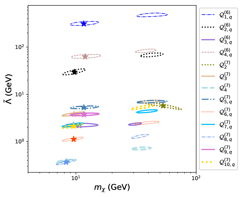
The results summarized in Table 4 can be understood in terms of a combination of kinematics, mainly driven by the cosine transform of the halo function defined in Eq. (2.23), and dynamics, determined instead by the correspondence between each relativistic model coupling and its non-relativistic limit, as summarized in Table 2.

To illustrate the role of the halo function in the kinematics of the scattering process, in Fig. 4 we plot the function $\eta_{m}(v)$. In particular, if in Eq. (2.21) the response function ${\cal R}$ does not show a strong energy dependence induced by the nuclear form factor, or, as in the case of the ${\cal O}_{7}$ or ${\cal O}_{14}$ NR operators, an explicit dependence on the velocity $v$ through a non–vanishing $R_{1k}^{\tau\tau^{\prime}}$ (see Eq. (2.12)) it is the $\eta_{m}(v)$ halo function that drives the energetic spectral shape of the modulation amplitude, and the latter can well reproduce the maximum observed above 2 keVee (see Fig. 2), once the $v$ range close to $\simeq$340 km/sec (for our choice of astrophysical parameters) is mapped to recoil energies around $\simeq$ 3 keVee through Eq. (2.11). Indeed, with a few exceptions discussed below, this is the mechanism that allows to achieve most of the acceptable $\chi^{2}$’s listed in Table 4. However, due to the different kinematics of the two processes, the energy range of the observed maximum corresponds to two different values of $m_{\chi}$ for WIMP–sodium and WIMP–iodine scattering. This explains the systematic presence of two minima in the $\chi^{2}$.

Moreover, in Fig. 4 the shaded areas represent the range of $v$ contributing to the DAMA modulated amplitudes between 1 keVee and 6 keVee for WIMP-sodium scattering (red) and WIMP–iodine scattering (green) in the specific example of the interaction term ${\cal Q}^{(6)}_{1,q}$ and in the the corresponding two minima of Table 4 (such $v$ ranges are defined as the intervals where in Eq. (2.21) the response function ${\cal R}(v)$ is different from zero). In particular, in Fig. 4(a), where the shaded areas are shown for the low–mass minimum, one can see that scattering off iodine is driven to $v$ values very close to the escape velocity ( for this reason it is not visible). Indeed, in such case scattering off iodine is kinematically accessible only below 2 keVee, while above that energy sodium alone contributes to the expected signal. On the other hand, Fig. 4(b) shows that in the high–mass minimum both targets contribute. However, in this case sodium is pushed down to low $v$ values, where the the modulation amplitude is suppressed.

As a consequence of the above discussion, the goodness–of–fit of the DAMA modulation amplitudes at low WIMP mass is sensitive to both WIMP–iodine and WIMP–sodium scattering, and so to the scaling between the two corresponding cross sections [50, 23, 51]. Indeed, in such case, provided that such hierarchy is not too large, a good fit can be attained since the energy dependence of the modulation amplitude is mostly driven by the $\eta_{m}(v)$ halo function and is only slightly modified above 2 keVee by the sodium form factor, which has a mild additional energy dependence due to the small size target and the sensitivity to smaller recoil energies at fixed electron–equivalent ones compared to iodine due to the larger quenching factor. On top of that, below 2 keVee WIMP–iodine scattering can provide a nice fit to the modulation amplitude measured by DAMA in the first energy bin: indeed, it is for this reason that in Table 4 most of the absolute minima correspond to the low WIMP mass solution. Among the different NR operators of Table 1 the case of a standard SI cross section, which corresponds to the NR operator $\mathcal{O}_{1}$, shows the largest hierarchy between the WIMP–iodine and WIMP–sodium cross sections, since they depend on the nuclear response function $W^{\tau\tau^{\prime}}_{M}$ (see Table 3) which scales with the mass numbers of the two targets. This makes it hard to fit WIMP–sodium scattering above 2 keVee without overestimating the WIMP–iodine process at lower energy unless the non–relativistic couplings $c^{n}_{j}$/$c^{p}_{j}$ off neutrons and protons are tuned to suppress the WIMP–iodine cross section, as pointed out in [50, 23, 52]. In particular, by combining the information contained in Table 2 and Table 3 one can notice that nine out of the sixteen relativistic effective models of Table 4 take contribution from the $W^{\tau\tau^{\prime}}_{TM}$ nuclear response function: ${\cal Q}_{1}^{(5)}$, ${\cal Q}_{2}^{(5)}$, ${\cal Q}_{1}^{(6)}$, ${\cal Q}_{1}^{(6)}$, ${\cal Q}_{1}^{(7)}$, ${\cal Q}_{2}^{(7)}$, ${\cal Q}_{5,q}^{(7)}$, ${\cal Q}_{6,q}^{(7)}$ and ${\cal Q}_{10,q}^{(7)}$. In particular, four of such operators correspond to effective interactions between the WIMP and gauge bosons (the photon and the gluon) for which the ratio between the non–relativistic couplings $c^{n}_{j}$/$c^{p}_{j}$ is fixed, and cannot be tuned to reduce the $\chi^{2}$: ${\cal Q}_{1}^{(5)}$, ${\cal Q}_{2}^{(5)}$, ${\cal Q}_{1}^{(7)}$ and ${\cal Q}_{2}^{(7)}$. Indeed, at low WIMP mass model ${\cal Q}_{1}^{(7)}$ has $\chi^{2}$=22.32 and ${\cal Q}_{2}^{(7)}$ has $\chi^{2}$=44.08, while the $\chi^{2}$ for models ${\cal Q}_{1}^{(5)}$ and ${\cal Q}_{2}^{(5)}$ is even higher, since they have the additional feature that the $1/q^{2}$ propagator further enhances the expected modulation amplitudes in the first two energy bins (for such long–range interactions this implies that also the $\chi^{2}$ at large WIMP masses is not acceptable). On the other hand the interactions ${\cal Q}_{1,q}^{(6)}$, ${\cal Q}_{2,q}^{(6)}$, ${\cal Q}_{5,q}^{(7)}$, ${\cal Q}_{6,q}^{(7)}$ and ${\cal Q}_{10,q}^{(7)}$ allow to tune the $r$ parameter to suppress the iodine contribution, leading to an acceptable $\chi^{2}$. Finally, the remaining seven interactions ${\cal Q}_{3}^{(6)}$, ${\cal Q}_{4}^{(6)}$, ${\cal Q}_{3}^{(7)}$, ${\cal Q}_{4}^{(7)}$, ${\cal Q}_{7}^{(7)}$, ${\cal Q}_{8}^{(7)}$ and ${\cal Q}_{9}^{(7)}$ achieve a good $\chi^{2}$ at small $m_{\chi}$ without any particular tuning because they are all driven by SD type nuclear form factors (i.e. $W^{\tau\tau^{\prime}}_{T\Sigma^{\prime\prime}}$ and/or $W^{\tau\tau^{\prime}}_{T\Sigma^{\prime}}$) for which no large hierarchy is observed in the first place between the WIMP–iodine and the WIMP–sodium cross sections.

As far as the large–mass minima of Table 4 are concerned, as explained above they correspond to the situation when WIMP–iodine scattering maps the maximum of the halo function $\eta_{m}(v)$ at $v\simeq$ 340 km/sec to recoil energies $\simeq$ 3 keV. In this case to get an acceptable fit the WIMP–sodium scattering process is not relevant, since, as shown in Fig. 4(b), for such WIMP masses it is driven to values of $v$ where its contribution to the modulation is suppressed. As a consequence, in the high–mass minima the modulation amplitudes are sensitive to WIMP–iodine scattering alone, while the hierarchy between the WIMP–sodium and WIMP–iodine cross sections does not play a significant role. In this case, however, another effect kicks in: due to the large size and the small quenching of the iodine target all the corresponding nuclear form factors $W^{\tau\tau^{\prime}}_{Tk}$ show a much steeper energy dependence compared to that of sodium. This additional energy dependence in the WIMP response function ${\cal R}$ alters the spectrum provided by the $\eta_{m}(v)$ halo function alone spoiling the goodness-of-fit at large WIMP masses, unless some mechanism is active to reduce it. In the models where an acceptable $\chi^{2}$ is achieved at large WIMP mass this mechanism is provided by an explicit momentum suppression in the WIMP response function $R_{k}^{\tau\tau^{\prime}}$ and/or (in the case of WIMP–quark interactions driven by $W^{\tau\tau^{\prime}}_{TM}$) by a tuning of the $c^{n}/c^{p}$ ratio.

In particular this explains why, out of the seven models with a momentum–suppressed SD type interaction (${\cal Q}_{3,q}^{(6)}$ and ${\cal Q}_{9,q}^{(7)}$, ${\cal Q}_{4,q}^{(6)}$, ${\cal Q}_{3}^{(7)}$, ${\cal Q}_{4}^{(7)}$, ${\cal Q}_{7,q}^{(7)}$ and ${\cal Q}_{8,q}^{(7)}$) all achieve a good $\chi^{2}$ at large WIMP masses with the exception of ${\cal Q}_{3,q}^{(6)}$ and ${\cal Q}_{9,q}^{(7)}$. It is worth noting that this implies that for ${\cal Q}_{4,q}^{(6)}$ a tuning of the $r$ parameter to enhance the ${\cal O}_{6}$ contribution ($q^{4}$ suppressed) compared to ${\cal O}_{4}$ (with no momentum suppression) is required to achieve a good $\chi^{2}$. Indeed, the ${\cal O}_{4}$ operator (i.e. a standard, SD interaction) has already been shown to yield a bad fit at large $m_{\chi}$ to the DAMA data [23]. This also explains why ${\cal Q}_{9,q}^{(7)}$, that corresponds to the NR operator ${\cal O}_{4}$ alone (again, see Table 2) yields a bad $\chi^{2}$ . On the other hand, the operator ${\cal Q}^{(6)}_{3,q}$ corresponds to a combination of ${\cal O}_{7}$ and ${\cal O}_{9}$, with the latter suppressed at large $m_{\chi}$ (see Table 2) so that in this case the contribution of ${\cal O}_{7}$ turn out to be sizeable. However (see Table 3 and Eq. (2.12)) the WIMP response function $R^{\tau\tau^{\prime}}_{k}$ of ${\cal O}_{7}$ shows in this case an explicit dependence on $v^{2}$ that spoils the fit (the same was observed in the fit of the ${\cal O}_{7}$ operator of Ref. [23]). For the five models that depend on $W^{\tau\tau^{\prime}}_{TM}$ and that correspond to effective interactions of the WIMP to quarks (${\cal Q}_{1,q}^{(6)}$, ${\cal Q}_{2,q}^{(6)}$, ${\cal Q}_{5,q}^{(7)}$, ${\cal Q}_{6,q}^{(7)}$ and ${\cal Q}_{10,q}^{(7)}$) besides momentum suppression, when present, the ratio of the non–relativistic couplings $c^{n}_{j}$/$c^{p}_{j}$ can be tuned to reduce the steepness of the iodine SI form factor and achieve an acceptable $\chi^{2}$. Such dependence on $c^{n}/c^{p}$ is not present for the two WIMP–gluon effective interactions ${\cal Q}_{1,q}^{(7)}$ and ${\cal Q}_{2,q}^{(7)}$: the former has no momentum suppression either, and so yields a a bad $\chi^{2}$, while the latter is momentum suppressed, so corresponds to an acceptable goodness–of–fit.

References

- [1] S. Chang, A. Pierce, and N. Weiner, Momentum Dependent Dark Matter Scattering, JCAP 1001 (2010) 006, [arXiv:0908.3192].
- [2] B. A. Dobrescu and I. Mocioiu, Spin-dependent macroscopic forces from new particle exchange, JHEP 11 (2006) 005, [hep-ph/0605342].
- [3] J. Fan, M. Reece, and L.-T. Wang, Non-relativistic effective theory of dark matter direct detection, JCAP 1011 (2010) 042, [arXiv:1008.1591].
- [4] R. J. Hill and M. P. Solon, WIMP-nucleon scattering with heavy WIMP effective theory, Phys. Rev. Lett. 112 (2014) 211602, [arXiv:1309.4092].
- [5] V. Gluscevic and A. H. G. Peter, Understanding WIMP-baryon interactions with direct detection: A Roadmap, JCAP 1409 (2014), no. 09 040, [arXiv:1406.7008].
- [6] M. Cirelli, E. Del Nobile, and P. Panci, Tools for model-independent bounds in direct dark matter searches, JCAP 1310 (2013) 019, [arXiv:1307.5955].
- [7] S. Chang, R. Edezhath, J. Hutchinson, and M. Luty, Effective WIMPs, Phys. Rev. D89 (2014), no. 1 015011, [arXiv:1307.8120].
- [8] R. Catena, Prospects for direct detection of dark matter in an effective theory approach, JCAP 1407 (2014) 055, [arXiv:1406.0524].
- [9] R. Catena, Dark matter directional detection in non-relativistic effective theories, JCAP 1507 (2015), no. 07 026, [arXiv:1505.06441].
- [10] R. Catena and P. Gondolo, Global fits of the dark matter-nucleon effective interactions, JCAP 1409 (2014), no. 09 045, [arXiv:1405.2637].
- [11] SuperCDMS Collaboration, K. Schneck et al., Dark matter effective field theory scattering in direct detection experiments, Phys. Rev. D91 (2015), no. 9 092004, [arXiv:1503.03379].
- [12] R. Catena and P. Gondolo, Global limits and interference patterns in dark matter direct detection, JCAP 1508 (2015), no. 08 022, [arXiv:1504.06554].
- [13] H. Rogers, D. G. Cerdeno, P. Cushman, F. Livet, and V. Mandic, Multidimensional effective field theory analysis for direct detection of dark matter, Phys. Rev. D95 (2017), no. 8 082003, [arXiv:1612.09038].
- [14] XENON Collaboration, E. Aprile et al., Effective field theory search for high-energy nuclear recoils using the XENON100 dark matter detector, Phys. Rev. D96 (2017), no. 4 042004, [arXiv:1705.02614].
- [15] CRESST Collaboration, G. Angloher et al., Limits on Dark Matter Effective Field Theory Parameters with CRESST-II, Eur. Phys. J. C79 (2019), no. 1 43, [arXiv:1809.03753].
- [16] R. J. Hill and M. P. Solon, Universal behavior in the scattering of heavy, weakly interacting dark matter on nuclear targets, Phys. Lett. B707 (2012) 539–545, [arXiv:1111.0016].
- [17] R. J. Hill and M. P. Solon, Universal behavior in the scattering of heavy, weakly interacting dark matter on nuclear targets, Phys. Lett. B707 (2012) 539–545, [arXiv:1111.0016].
- [18] M. Hoferichter, P. Klos, and A. Schwenk, Chiral power counting of one- and two-body currents in direct detection of dark matter, Phys. Lett. B746 (2015) 410–416, [arXiv:1503.04811].
- [19] M. Hoferichter, P. Klos, J. Menéndez, and A. Schwenk, Analysis strategies for general spin-independent WIMP-nucleus scattering, Phys. Rev. D94 (2016), no. 6 063505, [arXiv:1605.08043].
- [20] F. Bishara, J. Brod, B. Grinstein, and J. Zupan, From quarks to nucleons in dark matter direct detection, JHEP 11 (2017) 059, [arXiv:1707.06998].
- [21] S. Scopel and K. Yoon, A systematic halo-independent analysis of direct detection data within the framework of Inelastic Dark Matter, JCAP 1408 (2014) 060, [arXiv:1405.0364].
- [22] S. Scopel, K.-H. Yoon, and J.-H. Yoon, Generalized spin-dependent WIMP-nucleus interactions and the DAMA modulation effect, JCAP 1507 (2015), no. 07 041, [arXiv:1505.01926].
- [23] S. Kang, S. Scopel, G. Tomar, and J.-H. Yoon, DAMA/LIBRA-phase2 in WIMP effective models, JCAP 1807 (2018), no. 07 016, [arXiv:1804.07528].
- [24] S. Kang, S. Scopel, and G. Tomar, Probing DAMA/LIBRA in the full parameter space of WIMP effective models of inelastic scattering, Phys. Rev. D99 (2019) 103019, [arXiv:1902.09121].
- [25] COSINE-100 Collaboration, G. Adhikari et al., Search for a Dark Matter-Induced Annual Modulation Signal in NaI(Tl) with the COSINE-100 Experiment, Phys. Rev. Lett. 123 (2019), no. 3 031302, [arXiv:1903.10098].
- [26] COSINE-100, The Sogang Phenomenology Group Collaboration, G. Adhikari et al., COSINE-100 and DAMA/LIBRA-phase2 in WIMP effective models, JCAP 1906 (2019), no. 06 048, [arXiv:1904.00128].
- [27] J. Amaré et al., First Results on Dark Matter Annual Modulation from the ANAIS-112 Experiment, Phys. Rev. Lett. 123 (2019), no. 3 031301, [arXiv:1903.03973].
- [28] A. L. Fitzpatrick, W. Haxton, E. Katz, N. Lubbers, and Y. Xu, The Effective Field Theory of Dark Matter Direct Detection, JCAP 1302 (2013) 004, [arXiv:1203.3542].
- [29] N. Anand, A. L. Fitzpatrick, and W. C. Haxton, Weakly interacting massive particle-nucleus elastic scattering response, Phys. Rev. C89 (2014), no. 6 065501, [arXiv:1308.6288].
- [30] R. Catena, A. Ibarra, and S. Wild, DAMA confronts null searches in the effective theory of dark matter-nucleon interactions, JCAP 1605 (2016), no. 05 039, [arXiv:1602.04074].
- [31] J. Goodman, M. Ibe, A. Rajaraman, W. Shepherd, T. M. P. Tait, and H.-B. Yu, Constraints on Dark Matter from Colliders, Phys. Rev. D82 (2010) 116010, [arXiv:1008.1783].
- [32] M. R. Buckley, Using Effective Operators to Understand CoGeNT and CDMS-Si Signals, Phys. Rev. D88 (2013), no. 5 055028, [arXiv:1308.4146].
- [33] A. De Simone and T. Jacques, Simplified models vs. effective field theory approaches in dark matter searches, Eur. Phys. J. C76 (2016), no. 7 367, [arXiv:1603.08002].
- [34] A. Belyaev, E. Bertuzzo, C. Caniu Barros, O. Eboli, G. Grilli Di Cortona, F. Iocco, and A. Pukhov, Interplay of the LHC and non-LHC Dark Matter searches in the Effective Field Theory approach, Phys. Rev. D99 (2019), no. 1 015006, [arXiv:1807.03817].
- [35] J. Brod, A. Gootjes-Dreesbach, M. Tammaro, and J. Zupan, Effective Field Theory for Dark Matter Direct Detection up to Dimension Seven, JHEP 10 (2018) 065, [arXiv:1710.10218].
- [36] S. Kang, S. Scopel, G. Tomar, and J.-H. Yoon, On the sensitivity of present direct detection experiments to WIMP–quark and WIMP–gluon effective interactions: A systematic assessment and new model–independent approaches, Astropart. Phys. 114 (2020) 80–91, [arXiv:1810.00607].
- [37] E. Del Nobile, Complete Lorentz-to-Galileo dictionary for direct dark matter detection, Phys. Rev. D98 (2018), no. 12 123003, [arXiv:1806.01291].
- [38] E. Del Nobile, G. B. Gelmini, P. Gondolo, and J.-H. Huh, Direct detection of Light Anapole and Magnetic Dipole DM, JCAP 1406 (2014) 002, [arXiv:1401.4508].
- [39] S. Kang, S. Scopel, G. Tomar, J.-H. Yoon, and P. Gondolo, Anapole Dark Matter after DAMA/LIBRA-phase2, JCAP 1811 (2018), no. 11 040, [arXiv:1808.04112].
- [40] F. Bishara, J. Brod, B. Grinstein, and J. Zupan, DirectDM: a tool for dark matter direct detection, arXiv:1708.02678.
- [41] S. Kang, S. Scopel, G. Tomar, and J.-H. Yoon, Present and projected sensitivities of Dark Matter direct detection experiments to effective WIMP-nucleus couplings, Astropart. Phys. 109 (2019) 50–68, [arXiv:1805.06113].
- [42] R. Catena and B. Schwabe, Form factors for dark matter capture by the Sun in effective theories, JCAP 1504 (2015), no. 04 042, [arXiv:1501.03729].
- [43] S. E. Koposov, H.-W. Rix, and D. W. Hogg, Constraining the Milky Way potential with a 6-D phase-space map of the GD-1 stellar stream, Astrophys. J. 712 (2010) 260–273, [arXiv:0907.1085].
- [44] T. Piffl et al., The RAVE survey: the Galactic escape speed and the mass of the Milky Way, Astron. Astrophys. 562 (2014) A91, [arXiv:1309.4293].
- [45] E. Del Nobile, G. Gelmini, P. Gondolo, and J.-H. Huh, Generalized Halo Independent Comparison of Direct Dark Matter Detection Data, JCAP 1310 (2013) 048, [arXiv:1306.5273].
- [46] R. Bernabei et al., Searching for WIMPs by the annual modulation signature, Phys. Lett. B424 (1998) 195–201.
- [47] DAMA Collaboration, R. Bernabei et al., First results from DAMA/LIBRA and the combined results with DAMA/NaI, Eur. Phys. J. C56 (2008) 333–355, [arXiv:0804.2741].
- [48] DAMA, LIBRA Collaboration, R. Bernabei et al., New results from DAMA/LIBRA, Eur. Phys. J. C67 (2010) 39–49, [arXiv:1002.1028].
- [49] R. Bernabei et al., First Model Independent Results from DAMA/LIBRA–Phase2, Universe 4 (2018), no. 11 116, [arXiv:1805.10486]. [At. Energ.19,307(2018)].
- [50] S. Baum, K. Freese, and C. Kelso, Dark Matter implications of DAMA/LIBRA-phase2 results, Phys. Lett. B789 (2019) 262–269, [arXiv:1804.01231].
- [51] G. Angloher et al., The COSINUS project - perspectives of a NaI scintillating calorimeter for dark matter search, Eur. Phys. J. C76 (2016), no. 8 441, [arXiv:1603.02214].
- [52] F. Kahlhoefer, F. Reindl, K. Schäffner, K. Schmidt-Hoberg, and S. Wild, Model-independent comparison of annual modulation and total rate with direct detection experiments, JCAP 1805 (2018), no. 05 074, [arXiv:1802.10175].
- [53] XENON Collaboration, E. Aprile et al., Dark Matter Search Results from a One Ton-Year Exposure of XENON1T, Phys. Rev. Lett. 121 (2018), no. 11 111302, [arXiv:1805.12562].
- [54] PICO Collaboration, C. Amole et al., Dark Matter Search Results from the Complete Exposure of the PICO-60 C3F8 Bubble Chamber, Phys. Rev. D100 (2019), no. 2 022001, [arXiv:1902.04031].
- [55] XENON Collaboration, E. Aprile et al., Signal Yields of keV Electronic Recoils and Their Discrimination from Nuclear Recoils in Liquid Xenon, Phys. Rev. D97 (2018), no. 9 092007, [arXiv:1709.10149].
- [56] XENON100 Collaboration, E. Aprile et al., Likelihood Approach to the First Dark Matter Results from XENON100, Phys. Rev. D84 (2011) 052003, [arXiv:1103.0303].