Disorder driven phase transitions in weak AIII topological insulators
Abstract
The tenfold classification of topological phases enumerates all strong topological phases for both clean and disordered systems. These strong topological phases are connected to the existence of robust edge states. However, in addition to the strong topological phases in the tenfold classification, there exist weak topological phases whose properties under disorder are less well understood. It is unknown if the weak topological indices can be generalized for arbitrary disorder, and the physical signatures of these indices is not known. In this paper, we study disordered models of the two dimensional weak AIII insulator. We demonstrate that the weak invariants can be defined at arbitrary disorder, and that these invariants are connected to the presence or absence of bound charge at dislocation sites.
I Introduction
The tenfold periodic table of topological phases enumerates all possible strong topological phases that are protected by internal symmetries and robust against disorderSchnyder et al. 2008; Kitaev 2009; Qi et al. 2008; Ryu et al. 2010; Chiu et al. 2016. The ten symmetry classes are distinguished by the presence or absence of time-reveral (), charge-conjugation (), and chiral () symmetry. Within a given symmetry class, the insulating phases of Hamiltonians are categorized by a topological invariant of that symmetry class, i.e., a quantized index that can be calculated from the many-body ground state of the Hamiltonian. Strong topological phases exhibit protected gapless edge modes that cannot be gapped by symmetry-preserving surface perturbations and are inherently robust to symmetry-preserving disorderBernevig and Hughes 2013; Hasan and Kane 2010; Qi and Zhang 2011.
Besides the strong topological phases enumerated in the tenfold periodic table, there also exist weak topological phasesFu et al. 2007; Roy 2009; Moore and Balents 2007; Kitaev 2009. These phases nominally require lattice translation symmetry for their protection and can be viewed as “stacks” of lower dimensional topological insulators. The corresponding weak topological invariants are formed by averaging lower-dimensional strong topological invariants across the stack. For example, in the chiral-symmetric AIII class, the tenfold periodic table shows there exists a strong -valued topological index for 1D systems, the winding number (see below for further discussion of ), and no strong topological index for 2D systems. However, a 2D system formed from a stack of 1D chains with will have a weak topological index given by the average winding, . Weak topological phases also exhibit gapless edge modes for particular edge terminations that are compatible with the stacking direction, and additionally bind gapless states at crystalline defects such as dislocationsRan et al. 2009; Teo and Kane 2010; Teo and Hughes 2017.
Explicit expressions for calculating the strong topological invariant are generally given in terms of integrals over the Brillouin zone, and thus seemingly require translational invariance. However, the use of momentum space is just a basis choice, and formulas for the strong topological invariants in most symmetry classes have subsequently been generalized to real-space formulas that apply even to disordered systems Prodan et al. 2010; Loring and Hastings 2011; Mondragon-Shem et al. 2014; Prodan and Schulz-Baldes 2016a; Prodan 2017; Schulz-Baldes 2016; Prodan and Schulz-Baldes 2016b; Prodan et al. 2013. These real-space topological invariants recover the usual invariants when applied to a translationally invariant system. Furthermore, they are stable against weak disorder, are quantized even in the presence of strong disorder, and many of them can change values only if delocalized states exist at the Fermi level.
Ref. Prodan and Schulz-Baldes 2016b also established real-space formulae for weak topological invariants, and demonstrated that the corresponding invariants were quantized and stable for weak disorder as long as the spectral gap remains open. Recent mathematical work using KK-theoryProdan and Schulz-Baldes 2016c and semifinite index theoryBourne and Schulz-Baldes 2018 have also suggested formulae to calculate real-space weak topological invariants and demonstrated their quantization and stability under weak disorder. However, in all cases the properties of these weak topological invariants under strong disorder are not known.
In this paper, we explicitly study some classes of weak topological insulators in weak and strong disorder regimes. We define our weak topological invariants by directly apply the corresponding formulae for strong invariants in lower dimensions, as was suggested in Prodan and Schulz-Baldes 2016b. Our focus will be on 2D insulators in class AIII where the previously-knownMondragon-Shem et al. 2014 real-space formula for the 1D winding number allows us to compute the average 2D winding , by treating the 2D system as a 1D system with a width In this approach, the stability of these indices for weak disorder immediately follows from results on the corresponding strong invariants. However, the behavior at strong disorder is still not known. The theorems in Refs. Prodan and Schulz-Baldes 2016a; Prodan 2017; Schulz-Baldes 2016; Prodan and Schulz-Baldes 2016b establish that the strong invariants are quantized to integer values, but this only proves that a weak invariant like is quantized in units of at strong disorder, not that is itself an integer. Thus at strong disorder the quantization could vanish in the thermodynamic limit.
Using our real-space invariants, we study the phase diagrams of two models of the chiral-symmetric AIII class in two dimensions. In two dimensions, this class has two weak topological invariants, and , and no strong topological invariants. We confirm through computations of the weak topological invariants, and numerical transfer matrix methods, that the weak topological indices are robust against weak disorder. We also demonstrate numerically that the weak invariant remains quantized (in integer units) even at strong disorder when the Fermi level lies in a region of localized eigenstates, a result that has no known analytic proof. We show that generically, the disorder-driven phase transition in 2D is strikingly different from the 1D strong-topological versionMondragon-Shem et al. 2014; Song and Prodan 2014. Rather than a sharp phase boundary separating regions of different winding, there is a continuous transition region of delocalized states where the averaged winding varies smoothly between different values; this is reminiscent of a Dirac semi-metal phase separating the weak topological phase and trivial phase that could appear in the clean limit. Finally, we demonstrate a connection between the real-space weak topological invariant and physical observables, namely the electronic polarization and the bound charge at a dislocation.
II Background
To begin, we review the topological properties the AIII class, for both clean and disordered systems. We pay particular attention to the AIII class in 1D and 2D, which will be relevant for our work.
The AIII class is defined to be the set of all Hamiltonians that anticommute with an on-site unitary operator satisfying , called the chiral symmetry operator. This implies that
| (1) |
An immediate consequence of this equation is that the spectrum of is symmetric about , since if is an eigenstate of with energy , then is an eigenstate of with energy . The Fermi energy is assumed to be , which is compatible with the chiral symmetry and equivalent to assuming half filling due to the symmetry of the spectrum.
A simple example of a chiral symmetry operator in tight-binding models is the sublattice operator. For a given bipartite tight-binding lattice, we may divide the lattice into two sublattices A and B. In terms of this division, we define a sublattice operator that flips the sign of a single sublattice
Clearly . A simple calculation shows that whenever does not include hoppings within a single sublattice, such as . The examples of such tight-binding Hamiltonians that we will study are illustrated in Fig. 1. Each of these lattice models is bipartite, and their chiral symmetry operator will be the corresponding sublattice operator.
For translationally invariant systems in 1D we can define the topological invariant in the AIII class as follows. First, Eq. 1 can be expressed in -space for the Bloch Hamiltonian as
| (2) |
Since , the eigenvalues of are . If satisfies , then Eq. 1 implies . In other words, takes eigenstates of to eigenstates of , and thus takes an off-block-diagonal form when expressed in the basis of eigenstates:
| (3) |
for some operator . The 1D winding number invariant takes the form:
| (4) |
Ref. Mondragon-Shem et al. 2014 introduced a covariant real-space generalization of to AIII systems without translational symmetry. The key ingredient in defining the real-space topological invariant is a “flat band Hamiltonian” defined by
| (5) |
where is the projector onto the occupied states. By the same reasoning that led to Eq. 3, when written in a basis of eigenstates of , this flat-band Hamiltonian again takes an off-block-diagonal form
| (6) |
where . In terms of , the real-space generalization of Eq. 4 is given by
| (7) |
where is the number of unit cells in the -direction, and is the position operator.
This real-space reduces to the original winding number for translationally invariant systems. It has been demonstrated both numericallyMondragon-Shem et al. 2014; Song and Prodan 2014 and analyticallyProdan and Schulz-Baldes 2016a that is quantized to integer values even in the presence of strong disorder, provided only localized eigenstates exist at the Fermi level . In addition, Refs. Mondragon-Shem et al. 2014; Song and Prodan 2014 demonstrated that the transitions between different values of are sharp. From these properties we would expect the phase diagram in disorder-space to consist of regions of quantized separated by codimension-1 phase boundaries, and indeed, this is exactly what one finds in 1DMondragon-Shem et al. 2014; Song and Prodan 2014.
In the 2D AIII class, no strong topological invariants exist. However, there are topological classes in 2D determined by the weak topological indices and . These weak 2D topological indices can be defined in terms of the strong 1D topological index. We define by treating our two-dimensional system as a one-dimensional system that is infinite in the -direction and with width in the -direction. Then is defined as the 1D winding per unit width, . By dividing by , we ensure is well-defined in the limit . The weak invariant is defined similarly, by treating the system as a one-dimensional system infinite in the -direction and with width in the -direction, and dividing the resulting winding by . For translationally invariant gapped systems, and are still integers, despite the fact that the original integer-valued invariant has been divided by or . The indices and individually depend on the choice of basis vectors and of the lattice, but the vector quantity
| (8) |
is independent of the basis vectorsFu et al. 2007.
With these definitions the resulting real-space formulas for the weak invariants are then
| (9) | ||||
Note that while must be integer valued, and need not be, even if the Fermi level is in a region of localized states. Rather, since and are obtained from by dividing by and , respectively, is only guaranteed by Ref. Prodan and Schulz-Baldes 2016a to be quantized to integer multiples of , and similar for . In the thermodynamic limit, then, the can in principle take on any value in . One of the important results of this work will be demonstrating that when the Fermi level is in a region of localized eigenstates, the retain their quantization and are nonetheless still integers even as one approaches the thermodynamic limit.
III 2D AIII Models
The simplest way to form two-dimensional models with nontrivial weak indices is to stack 1D models with nontrivial . Our basic building block will be the chiral symmetric 1D Su-Schrieffer-Heeger (SSH) chainSu et al. 1979, the simplest example of an AIII topological insulator in 1D (Fig. 1a). The SSH chain has when , and otherwise. To create our 2D models, we first stack SSH chains, and then add some local inter-chain couplings that are allowed by the chiral (sublattice) symmetry.


The two 2D models we consider are illustrated in Figs. 1b and 1c. The two sublattices A and B are colored red and blue, respectively; note that there is no coupling between sites on the same sublattice, as required by chiral symmetry. Our first model, shown in Fig. 1b, is a two-band model given by a vertical stack of SSH chains in which nearest-neighbor unit cells are coupled in the vertical direction. Our second model, shown in Fig. 1c, is a four-band model given by two crossed stacks of SSH chains, with intracell couplings between the horizontal and vertical chains. While the pattern of hoppings may appear artificial, such hopping patterns can be realized experimentally in metamaterials, such as topolectric circuits Lee et al. 2018. In addition, for solid-state realizations the A and B sites don’t need correspond to physical lattice sites; they may refer to any degrees of freedom located in a unit cell11 1 One simple way to realize such a hopping pattern in a solid-state context is to consider a spinless superconductor with time-reversal symmetry . Then the product of time-reversal and particle-hole symmetry gives a chiral symmetryChiu et al. 2016. In this case, our corresponds to a superconductor with one lattice site per unit cell, the degrees of freedom A and B correspond to Bogoliubov quasiparticle operators , and coupling between them is forbidden simply by symmetry. Note that adding symmetry technically puts us in the BDI rather than AIII class, but the topological invariants of these two classes are identicalChiu et al. 2016; Song and Prodan 2014..
Written explicitly, the Hamiltonians are given by
| (10) |
| (11) |
In both models, the parameters and represent position dependent hoppings. We study disordered versions of translationally-invariant systems, so we choose hoppings via
| (12) |
Here, and are the hopping strengths in the clean limit, the and are independent random variables uniformly distributed in , and and are measures of the intracell and intercell disorder strengths, respectively.
In the clean limit, is gapped provided either or , and gapless otherwise. In the first gapped case , while in the second gapped case . Meanwhile, is gapped provided , or , or , and gapless otherwise. In the first gapped case, , while in the second and third gapped cases . The phase diagrams for each model in the clean limit are shown in Fig. 2. For our disordered systems we choose the initial parameters for and for . The parameters represent arbitrary points in the topological phase, and can be changed without affecting our conclusions. These points in the phase diagram are indicated by black crosses in Fig. 2, where it is apparent that we start with and for and , respectively. Note that systems with arbitrary can be formed from stacks of these two elementary models.


IV Disordered Weak Topological Insulators
IV.1 Behavior for finite-width systems
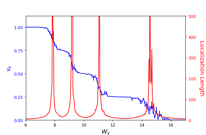
In order to connect our results to Refs. Mondragon-Shem et al. 2014; Song and Prodan 2014, we first explore the behavior of for disordered systems with finite in the limit . We can then treat our system as a thick 1D chain of width . From the work in Refs. Mondragon-Shem et al. 2014; Song and Prodan 2014, we expect that the 1D topological invariant given by Eq. 7 is quantized to integer values, except at points in in the phase diagram where the localization length at diverges. We also know that as , we should have , since in this limit the intracell terms in the Hamiltonian dominate, and we thus expect a trivial insulator. This can also be seen directly from Eq. 7, since in this limit commutes with . We thus expect that as we increase from 0, will decrease in some manner from to , and any drops in should be accompanied by diverging localization length diverges at In terms of our weak topological index we expect similar behavior. Namely, we expect at zero disorder, for , and decreases as we increase .
We show the results of our numerical calculations in Fig. 3 for with a width . We see that drops in steps of size , and these drops occur precisely when the localization length diverges. This result shows that the transition between a (finite-width) weak topological insulator and a trivial insulator is generically split into separate transitions in the presence of disorder, and each transition is accompanied by a diverging localization length in the -direction.
We these results in mind, we now want to consider novel features that may emerge in the limit. In this limit, we might expect that the isolated values of at which the localization length diverges coalesce into an interval (or, in the case of higher-dimensional disorder configuration space, a region) having a diverging localization length throughout. In such an interval (or region), the value of can change continuously. However, if there are intervals or regions in disorder-space where the localization length remains finite as , cannot change in these regions. When considering the limit , we will be interested in the following questions:
- •
Are there still sharp transitions between different values of as in Refs. Mondragon-Shem et al. 2014; Song and Prodan 2014, or do points with diverging localization length coalesce into a region of disorder space, allowing to change continuously in this region?
- •
Do there still exist regions of disorder-space where the localization length remains finite, where plateaus to a well-defined value as ?
- •
If there still exist regions of disorder-space with finite localization length, can plateau at any value, or does take on only integer values as in the clean limit?
IV.2 Disordered Phase Diagrams in the Thermodynamic Limit


In Figs. 4a and 5a we plot phase diagrams for models and , respectively, as a function of two disorder parameters. Here, as in Fig. 2, red (blue) represents . For both and , we find that is smooth as a function of disorder, and we do not see a sharp transition between values of that are quantized to integers. However, in both figures we find a region around zero disorder where remains quantized at 1 up to a finite value of disorder. In addition, in both cases we see “islands” at strong disorder where regains quantization; in the case of an island having appears at strong , and in the case of an island having appears at strong . Finally, at no point do we see plateaus at non-integer values that survive the limit.
Let us address possible concerns that the above features are just artifacts of finite-size effects. One might worry that the phase transition becomes sharp in the thermodynamic limit, or that the islands of quantized disappear. We can eliminate these possibilities by considering the localization length at . Because the topological invariant can only change when there are delocalized states at , computing the localization length at can constrain the points in the phase diagram where is allowed to change. To compute the localization length, we use a transfer-matrix method that numerically determines the localization length for samples which are finite in the direction, but arbitrarily large in Pichard and Sarma 1981. The results are plotted in Figs. 4(b-d) and 5(b-d) for progressively larger values of . In both cases, the behavior in the limit is readily apparent. We observe that delocalized states coalesce to densely fill regions of the disorder configuration space, but are excluded from the islands where we claim that remains quantized. These localization calculations demonstrate that, even in the limit, must remain quantized for weak disorder, as there are no delocalized states at weak disorder. It also demonstrates that no islands of stable, non-quantized values of appear in the phase diagram as , as the only regions we find without delocalized states are regions in which is integer-valued (i.e., and is not just an integer multiplying ).
Let us summarize these results. Our real-space weak invariants remain quantized at weak disorder that does not close the bulk gap, as in Refs. Prodan et al. 2013; Prodan and Schulz-Baldes 2016c; Bourne and Schulz-Baldes 2018. In our formulation, this is manifest because our formula for cannot change without delocalized states appearing at the , and at weak disorder the spectral gap remains open and cannot change. In addition, we have numerical evidence that the weak indices remain quantized even at strong disorder provided there exist no delocalized states at the Fermi level, something that analytic arguments have not yet established. We conjecture that this is generic, i.e., that and are quantized for any homogeneous disorder that obeys chiral symmetry and does not result in delocalized states at the Fermi level. We also find that there is a contiguous region of delocalized states separating the weak topological phase from the trivial insulator phase, and as we will see below, the properties of this critical region are reminiscent of those expected for an intermediate Dirac semimetal phase that separates the weak from the trivial phaseRamamurthy and Hughes 2015. In this phase, the metallic character is robust in a region of the phase diagram, and is protected from disorder by the fractional value of .
The quantization of at strong disorder allows us to identify highly-disordered systems as having protected weak topological properties. Indeed, once we connect to real-space observables (see below), the quantization of at strong disorder implies that even strongly disordered systems can exhibit stable, quantized properties that are protected by real-space weak topology.
IV.3 Signatures of Disordered Weak Topological Insulators
IV.3.1 Polarization and edge modes
For a clean AIII system, if we introduce a clean boundary perpendicular to , the invariant predicts the number of robust zero-energy modes (per ) localized at the boundary. These robust zero-energy modes are chiral, satisfying with the same sign for all the modes on the boundary. This implies that these states cannot be moved away from zero energy by any chiral-symmetric perturbation, since the matrix elements between them necessarily vanish: In addition to providing a spectroscopic signature of the weak topological phase these modes result in the manifestation of a boundary charge generated by a polarization given by where is the electric charge and we have assumed lattice constants are normalized to unity.
With the addition of weak disorder that does not close the bulk gap, still robustly predicts the number of edge modes, and thus can be associated with a bulk polarization. For stronger disorder, we cannot easily distinguish between the protected zero energy modes on the edges and the bulk zero energy modes. However, a signature of the zero energy modes remains. If we add a small chiral-symmetry (and inversion-symmetry) breaking term to the Hamiltonian, the charge density per unit length on an edge is given by , where the sign depends on the sign of . Remarkably, we find that this holds even for the case of fractional , when delocalized states exist at zero energy, similar to the well-defined polarization and boundary charge in a gapless 2D Dirac semi-metalRamamurthy and Hughes 2015. Therefore, the polarization of a sample with edges22 2 Note that we calculate the polarization with open boundary conditions through the surface charge. Methods for computing the polarization with periodic boundary conditions such as those of Refs. Resta 1998; Ortiz and Martin 1994 only give the dipole moment per length mod , and cannot determine the dipole moment per unit volume. still satisfies .
IV.3.2 Bound charge at dislocations
In clean systems, it is known that weak topological insulators have protected modes at edge (and in 3D, screw) dislocationsChiu et al. 2016; Teo and Kane 2010; Ran et al. 2009. In 2D AIII systems without disorder, a dislocation hosts a bound charge that obeys the relationship
| (13) |
where is the Burgers vectorKittel et al. 1976 of the dislocation, and is as the weak invariant defined in Eq. 8. For clean systems, this bound charge cannot be removed by (weak) disorder near the edge dislocation; thus, these modes are a possible signature of the weak topological phase even with bulk disorder.
We confirm this behavior persists in the presence of bulk disorder by calculating the charge density near an edge dislocation, as shown in Fig. 6. There, we plot the charge density near an edge dislocation for the points in the phase diagram indicated by black squares in Figs. 4a and 5a. We see that for both models there is a charge of bound to the defect in the phase, and no charge in the phase. Remarkably this is true even for the very strong disorder case shown in Fig. 6d where the system has for large values of disorder that are not perturbations around a clean limit. We conjecture that this behavior is generic, i.e., Eq. 13 remains valid for systems with arbitrary disorder, provided we are in a region of quantized where the localization length at is finite. We remark that in the region of delocalized states it was not possible to obtain reliable calculations of the localized dislocation charge, so the behavior of dislocations in this part of the phase diagram remains an open question.


V Discussion/Conclusion
By extending real-space formulas for the strong topological invariant, we have introduced a method to define real-space weak topological invariants for AIII systems. Our invariants are quantized at weak disorder, as in Refs. Prodan and Schulz-Baldes 2016c; Bourne and Schulz-Baldes 2018. By combining our real-space formula with a numerical transfer matrix method, we have also gone beyond those works and demonstrated that for the AIII class in regions without delocalized states at , the weak indices take on quantized values. In contrast to the 1D case, the weak topological indices do not transition at a critical value of disorder, but instead have a critical region where the topological index smoothly transitions between quantized plateaus. We conjecture that this behavior is generic for homogeneous disorder, although there are no known analytic proofs of the quantization of weak invariants in general. The critical region takes the place of the intermediate 2D Dirac semi-metal phase that separates trivial insulators from weak topological insulators in clean systems. Indeed, our results share some similarities with calculations done for disordered 3D Weyl semi-metals that are proximate to a weak topological insulator phaseShapourian and Hughes 2016. In addition, we have connected the weak invariants to real-space observables. Like the clean system, we see that nontrivial disordered systems bind a quantized amount of charge at dislocation cores at both weak and strong disorder. Such systems also display a quantized polarization. We conjecture that this behavior is also generic.
One could extend this method to weak topological phases in other symmetry classes and dimensions where the formula for the corresponding real-space strong topological index is known. In general, a combination of real-space calculations of the topological index and computation of the localization length at the Fermi level should be able to precisely map the phase diagram in disorder-space in many cases. It would also be interesting to see if the link between these weak topological indices and bound states at dislocations generalizes to other symmetry classes, for example the existence of chiral/helical states bound to 2D line defects in the 3D A/AII classesRan et al. 2009.
Acknowledgements
TLH thanks the National Science Foundation (NSF) grant DMR-1351895 (CAREER) for support. TLH also thanks the National Science Foundation under Grant No. NSF PHY-1748958(KITP) for partial support at the end stage of this work during the Topological Quantum Matter program. This work made use of the Illinois Campus Cluster, a computing resource that is operated by the Illinois Campus Cluster Program (ICCP) in conjunction with the National Center for Supercomputing Applications (NCSA) and which is supported by funds from the University of Illinois at Urbana-Champaign.
References
- Schnyder et al. (2008) A. P. Schnyder, S. Ryu, A. Furusaki, and A. W. W. Ludwig, Phys. Rev. B 78, 195125 (2008).
- Kitaev (2009) A. Kitaev, AIP Conf. Proc. 1134, 22 (2009).
- Qi et al. (2008) X.-L. Qi, T. L. Hughes, and S.-C. Zhang, Phys. Rev. B 78, 195424 (2008).
- Ryu et al. (2010) S. Ryu, A. P. Schnyder, A. Furusaki, and A. W. Ludwig, New J. Phys. 12, 065010 (2010).
- Chiu et al. (2016) C.-K. Chiu, J. C. Y. Teo, A. P. Schnyder, and S. Ryu, Rev. Mod. Phys. 88, 035005 (2016).
- Bernevig and Hughes (2013) B. A. Bernevig and T. L. Hughes, Topological insulators and topological superconductors (Princeton university press, 2013).
- Hasan and Kane (2010) M. Z. Hasan and C. L. Kane, Rev. Mod. Phys. 82, 3045 (2010).
- Qi and Zhang (2011) X.-L. Qi and S.-C. Zhang, Rev. Mod. Phys. 83, 1057 (2011).
- Fu et al. (2007) L. Fu, C. L. Kane, and E. J. Mele, Phys. Rev. Lett. 98, 106803 (2007).
- Roy (2009) R. Roy, Phys. Rev. B 79, 195322 (2009).
- Moore and Balents (2007) J. E. Moore and L. Balents, Phys. Rev. B 75, 121306(R) (2007).
- Ran et al. (2009) Y. Ran, Y. Zhang, and A. Vishwanath, Nat. Phys. 5, 298 (2009).
- Teo and Kane (2010) J. C. Y. Teo and C. L. Kane, Phys. Rev. B 82, 115120 (2010).
- Teo and Hughes (2017) J. C. Y. Teo and T. L. Hughes, Annu. Rev. Condens. Matter Phys. 8, 211 (2017).
- Prodan et al. (2010) E. Prodan, T. L. Hughes, and B. A. Bernevig, Phys. Rev. Lett. 105, 115501 (2010).
- Loring and Hastings (2011) T. A. Loring and M. B. Hastings, EPL 92, 67004 (2011).
- Mondragon-Shem et al. (2014) I. Mondragon-Shem, T. L. Hughes, J. Song, and E. Prodan, Phys. Rev. Lett. 113, 046802 (2014).
- Prodan and Schulz-Baldes (2016a) E. Prodan and H. Schulz-Baldes, J. Funct. Anal. 271, 1150 (2016a).
- Prodan (2017) E. Prodan, A computational non-commutative geometry program for disordered topological insulators (Springer, 2017).
- Schulz-Baldes (2016) H. Schulz-Baldes, Jahresber. Dtsch. Math.-Ver. 118, 247 (2016).
- Prodan and Schulz-Baldes (2016b) E. Prodan and H. Schulz-Baldes, Bulk and boundary invariants for complex topological insulators (Springer, 2016).
- Prodan et al. (2013) E. Prodan, B. Leung, and J. Bellissard, J. Phys. A 46, 485202 (2013).
- Prodan and Schulz-Baldes (2016c) E. Prodan and H. Schulz-Baldes, Rev. Math. Phys. 28, 1650024 (2016c).
- Bourne and Schulz-Baldes (2018) C. Bourne and H. Schulz-Baldes, in 2016 MATRIX Annals (Springer, 2018) pp. 203–227.
- Song and Prodan (2014) J. Song and E. Prodan, Phys. Rev. B 89, 224203 (2014).
- Su et al. (1979) W. P. Su, J. R. Schrieffer, and A. J. Heeger, Phys. Rev. Lett. 42, 1698 (1979).
- Lee et al. (2018) C. H. Lee, S. Imhof, C. Berger, F. Bayer, J. Brehm, L. W. Molenkamp, T. Kiessling, and R. Thomale, Commun. Phys. 1, 1 (2018).
- (28) One simple way to realize such a hopping pattern in a solid-state context is to consider a spinless superconductor with time-reversal symmetry . Then the product of time-reversal and particle-hole symmetry gives a chiral symmetryChiu et al. 2016. In this case, our corresponds to a superconductor with one lattice site per unit cell, the degrees of freedom A and B correspond to Bogoliubov quasiparticle operators , and coupling between them is forbidden simply by symmetry. Note that adding symmetry technically puts us in the BDI rather than AIII class, but the topological invariants of these two classes are identicalChiu et al. 2016; Song and Prodan 2014.
- Pichard and Sarma (1981) J. Pichard and G. Sarma, J. Phys. C 14, L127 (1981).
- Ramamurthy and Hughes (2015) S. T. Ramamurthy and T. L. Hughes, Phys. Rev. B 92, 085105 (2015).
- (31) Note that we calculate the polarization with open boundary conditions through the surface charge. Methods for computing the polarization with periodic boundary conditions such as those of Refs. Resta 1998; Ortiz and Martin 1994 only give the dipole moment per length mod , and cannot determine the dipole moment per unit volume.
- Kittel et al. (1976) C. Kittel et al., Introduction to solid state physics, Vol. 8 (Wiley New York, 1976).
- Shapourian and Hughes (2016) H. Shapourian and T. L. Hughes, Phys. Rev. B 93, 075108 (2016).
- Resta (1998) R. Resta, Phys. Rev. Lett. 80, 1800 (1998).
- Ortiz and Martin (1994) G. Ortiz and R. M. Martin, Phys. Rev. B 49, 14202 (1994).