Recovery of massless Dirac fermions at charge neutrality in strongly interacting twisted bilayer graphene with disorder

Consider two monolayer-graphene sheets stacked such that they are twisted relative to one another by an angle $\theta$, as shown in Fig. 3(a) (for an arbitrary angle $\theta$). The twist dramatically reduces the system’s translational symmetry. While true translational symmetry requires special commensurate angles, when the twist angle is small, an effective moiré translational symmetry emerges; the resulting triangular superlattice of orange AA regions, each surrounded by a hexagon of alternating AB and BA regions, is clearly visible in the cartoon of Fig. 3(a). In this case, the band structure at charge neutrality descends from the band structure of the individual graphene layers in a relatively straightforward manner when described in momentum space Bistritzer and MacDonald 2011; Lopes Dos Santos et al. 2007. Figure 3(b) shows the Brillouin zones (BZs) of the top and bottom graphene monolayers after applying a rotation by an angle $+\theta/2$ and $-\theta/2$, respectively. The reciprocal lattice vectors of the resulting moiré pattern are given by $\boldsymbol{G}_{\ell}=\mathcald{R}_{\theta/2}\left[\boldsymbol{\mathcald{G}}_{\ell}\right]-\mathcald{R}_{-\theta/2}\left[\boldsymbol{\mathcald{G}}_{\ell}\right]$ where $\boldsymbol{\mathcald{G}}_{1,2}$ denote the reciprocal lattice vectors of the unrotated graphene sheets and $\mathcald{R}_{\phi}[\boldsymbol{v}]$ rotates a vector $\boldsymbol{v}$ by an angle $\phi$. The length of the moiré reciprocal lattice vectors, $\left|\boldsymbol{G}_{\ell}\right|$, is therefore suppressed relative the graphene reciprocal lattice vectors by a factor of $2\sin\left(\theta/2\right)\sim\theta$, making it very small by assumption. Equivalently, the moiré lattice constant is enlarged by $\sim 1/\theta$ relative to the graphene lattice constant. We let $\pm{\boldsymbol{K}}{t}=\mathcald{R}_{\theta/2}[\pm{\boldsymbol{K}}]$ and $\pm{\boldsymbol{K}}{b}=\mathcald{R}_{-\theta/2}[\pm{\boldsymbol{K}}]$ denote the $\pm{\boldsymbol{K}}$ points of the top and bottom layers, respectively.

As tunnelling between the two layers turns on, states at momentum ${\boldsymbol{K}}{t}+{\boldsymbol{k}}$ on the top layer mix with those at momentum ${\boldsymbol{K}}{b}+{\boldsymbol{k}}+{\boldsymbol{q}}_{\ell}+\boldsymbol{G}$ on the top layer, where $\boldsymbol{G}$ is a moiré reciprocal lattice vector and ${\boldsymbol{q}}_{\ell}=\mathcald{R}_{2\pi(\ell-1)/3}\left[{\boldsymbol{K}}{t}-{\boldsymbol{K}}{b}\right]$, $\ell=1,2,3$ [see Fig. 3(b)]. Since the moiré BZ is much smaller than the BZ of monoloyer graphene, mixing states proximate to ${\boldsymbol{K}}$ with those proximate to $-{\boldsymbol{K}}$ is an extremely high-order tunnelling process; the two valleys of the original graphene monolayers thus effectively decouple. This decoupling is particularly convenient as it allows us to express the full band Hamiltonian $H_{\mathrm{cont}}$ as a sum of terms for the ${\boldsymbol{K}}$ and $-{\boldsymbol{K}}$ valleys: $H_{\mathrm{cont}}=H_{+}+H_{-}$. For convenience, we explicitly reproduce $H_{+}$ in Appendix A. Our ability to decompose the Hamiltonian into ${\boldsymbol{K}}$-valley sectors is equivalent to the emergence of a U(1) “valley” symmetry, which we denote U(1)_v.

In addition to moiré translations and U(1)_v, the continuum model preserves the SU(2)_s spin rotation symmetry (neglecting spin-orbit coupling), time reversal ${\mathcald{T}}$, ${\mathcald{C}}_{2}$ rotations by $\pi$, ${\mathcald{C}}_{3}$ rotations by $2\pi/3$, and a mirror symmetry ${\mathcald{M}}_{y}$ that takes $(x,y)\to(x,-y)$ and interchanges the two layers. The latter three should be regarded as emergent symmetries similar to U(1)_v. In our conventions the time-reversal operator ${\mathcald{T}}$ does not flip the electronic spins and accordingly obeys ${\mathcald{T}}^{2}=+1$. Both ${\mathcald{T}}$ and ${\mathcald{C}}_{2}$ interchange the two valleys and hence are not symmetries of the individual single-valley Hamiltonians $H_{\pm}$. Rather than keep track of these two symmetries separately, it is therefore convenient to consider ${\mathcald{T}}$ along with the composite operation ${\mathcald{C}}_{2}{\mathcald{T}}$—which commutes with U(1)_v.

The momenta ${\boldsymbol{K}}{t}$ and ${\boldsymbol{K}}{b}$ map to the corners of the moiré BZ. In what follows, we denote these momenta by $\pm{\boldsymbol{\kappa}}$ to distinguish them from the $\pm{\boldsymbol{K}}$-valleys of the microscopic graphene layers. Provided the ${\mathcald{C}}_{2}{\mathcald{T}}$ and ${\mathcald{C}}_{3}$ symmetries are present, the massless Dirac cones at ${\boldsymbol{K}}_{\mathcald{t},\mathcald{b}}$ for the microscopic graphene layers evolve into massless Dirac cones at $\pm{\boldsymbol{\kappa}}$ even once tunnelling is turned on. This crucial property follows from the fact that the Berry phase enclosed within any loop is quantized to 0 or $\pi$ ($\mathrm{mod}\,2\pi$) when ${\mathcald{C}}_{2}{\mathcald{T}}$ is preserved. Since a Dirac point necessarily exhibits Berry phase $\pi$, the Dirac cones at $+{\boldsymbol{\kappa}}$ and $-{\boldsymbol{\kappa}}$ are locally protected against a mass Kim et al. 2015; Po et al. 2018. Breaking ${\mathcald{C}}_{3}$ can shift the location of the Dirac cones, but cannot gap them. Importantly, since both cones in $H_{+}$ ($H_{-}$) descend from the Dirac cones at ${\boldsymbol{K}}{t,b}$ ($-{\boldsymbol{K}}{t,b}$) in a continuous fashion, they possess the same chirality de Gail et al. 2011; He et al. 2013—thereby obstructing the development of a two-band, single ${\boldsymbol{K}}$-valley tight-binding model in which all symmetries are realized in a local fashion Po et al. 2018; Po et al. 2019; Kang and Vafek 2018.

The previous subsection highlighted generic features of small-angle twisted-bilayer graphene. At the magic angle, the velocity of the massless Dirac fermions becomes very small, and the bands immediately above and below the charge neutrality point separate from the remaining bands by a finite energy (provided lattice relaxation is incorporated Nam and Koshino 2017; Koshino et al. 2018; Po et al. 2018); see Fig. 3(c). The resulting energetically isolated “flat bands” are each (essentially) four-fold degenerate, reflecting spin and valley degrees of freedom. We now describe the flat-band Hamiltonian by first focusing on the $+{\boldsymbol{K}}$ valley and subsequently incorporating the $-{\boldsymbol{K}}$ valley.

Let $c_{\alpha j}({\boldsymbol{k}})$ denote momentum-space annihilation operators associated with the flat bands at valley $+{\boldsymbol{K}}$; here $\alpha={\uparrow,\downarrow}$ is a spin index and $j=1,2$ is a band index. Reference Zou et al. 2018 showed that these operators can be defined such that they transform under ${\mathcald{C}}_{2}{\mathcald{T}}$ via

with Pauli matrices $\eta^{x,y,z}$ that act on the band indices. (Here and below we often suppress indices for notational simplicity.) It follows that the ${\mathcald{C}}_{2}{\mathcald{T}}$-invariant flat-band Hamiltonian takes the form

Next we project onto the massless Dirac fermions at $\pm{\boldsymbol{\kappa}}$ in the moire BZ by defining Dirac spinors $\psi_{1\alpha j}({\boldsymbol{q}})\sim c_{\alpha j}(+{\boldsymbol{\kappa}}+{\boldsymbol{q}})$ and $\psi_{2\alpha j}({\boldsymbol{q}})\sim c_{\alpha j}(-{\boldsymbol{\kappa}}+{\boldsymbol{q}})$ and retaining only small ${\boldsymbol{q}}$ modes. The fact that the massless Dirac cones exhibit the same chirality at $\pm{\boldsymbol{\kappa}}$ implies that $h_{x}(\pm{\boldsymbol{\kappa}}+{\boldsymbol{q}})\sim+q_{x}$ and $h_{y}(\pm{\boldsymbol{\kappa}}+{\boldsymbol{q}})\sim+q_{y}$. Upon shifting the energy such that $h_{0}(\pm{\boldsymbol{\kappa}})=0$ and reverting to real space, the low-energy Hamiltonian becomes

The Fermi velocity $v_{F}$ has been assumed isotropic and identical for both $\pm{\boldsymbol{\kappa}}$ Dirac cones, which is guaranteed when all symmetries outlined earlier are present.

An insulating phase at charge neutrality may only be obtained by either breaking the ${\mathcald{C}}_{2}{\mathcald{T}}$ symmetry or by closing the gap separating the flat bands and the dispersing bands Kim et al. 2015; Po et al. 2018. We focus entirely on the former scenario, which is straightforward to represent using the Dirac theory. Let $\tau^{x,y,z}$ and $\sigma^{x,y,z}$ denote Pauli matrices that respectively act on ${\boldsymbol{\kappa}}$-valley indices and spin indices. Mass terms then take the form $\psi^{\dagger}\eta^{z}M\psi$ with $M=\big\{\mathds{1},\sigma^{i},\tau^{i},\tau^{i}\sigma^{j}\big\}$. The Chern number for a given spin/valley sector depends on the relative sign of the masses gapping the ${\boldsymbol{\kappa}}$ and $-{\boldsymbol{\kappa}}$ Dirac cones. When both cones have the same-sign mass, the sector acquires Chern number $C=\pm 1$, whereas opposite-sign masses yield $C=0$. Consequently, mass terms with $M=\mathds{1},\,\sigma^{i}$ yield insulating bands with non-zero Chern number, while masses with $M=\tau^{i},\,\tau^{i}\sigma^{j}$ yield trivial insulating bands²² 2 Given the Hamiltonian $H_{D}$, the above conclusions regarding Chern number hold true regardless of the details of the high-energy theory from which it was derived. It is worth noting that for a single graphene sheet, expanding in small ${\boldsymbol{q}}$ the functions analogous to $h_{x,y}(\pm{\boldsymbol{\kappa}}+{\boldsymbol{q}})$ would not yield the low-energy Hamiltonian of Eq. (3). Instead, the two Dirac cones would possess opposite chirality..

We now restore the $-{\boldsymbol{K}}$ valley. In terms of the low-energy Dirac Hamiltonian, the chirality of the massless Dirac fermions in the $-{\boldsymbol{K}}$ valley is opposite that of the $+{\boldsymbol{K}}$ valley. Defining the spinor $\Psi=(\psi_{+},\psi_{-})^{T}$, where $\psi_{\pm}$ describe Dirac fermions in valley $\pm{\boldsymbol{K}}$, the full Dirac Hamiltonian may be written

where we introduced Pauli matrices $\mu^{x,y,z}$ that act on ${\boldsymbol{K}}$-valley indices. The presence of $\mu^{z}$ in the first term above implements the opposite-chirality requirement. Our discussion of the mass terms and the associated Chern numbers extends straightforwardly to the $\Psi$ fermions. For details see Appendix B. A notable consequence of the opposing chiralities of the $\pm{\boldsymbol{K}}$ valleys is that a mass term $\Psi^{\dagger}\eta^{z}\Psi=\psi_{+}^{\dagger}\eta^{z}\psi_{+}+\psi_{-}^{\dagger}\eta^{z}\psi_{-}$ generates an insulator with $C=+1$ for the $+{\boldsymbol{K}}$ valley and $C=-1$ for the $-{\boldsymbol{K}}$ valley (or vice versa depending on the overall sign of the mass term). These insulators correspond to the quantum valley Hall states that play a prominent role in this paper.

In the following sections, we use the operator $\psi$ when restricting our discussion to a single ${\boldsymbol{K}}$-valley. We suppress the “$\pm$” indices in such cases but assume for concreteness that the $+{\boldsymbol{K}}$ valley is being considered (as in the beginning of this subsection). We reserve use of $\Psi$ for occasions when both valleys are discussed simultaneously.

It is useful to review the specific types of disorder that are believed to be most relevant to experiments, though we attempt to keep the majority of our discussion as general as possible. Charge disorder appears to be quite low: Refs. Cao et al. 2018b; Yankowitz et al. 2019; Uri et al. 2019 estimate charge-carrier inhomogeneity in the range $\delta n\sim{1-2\times 10^{10}\,\mathrm{\text{cm}^{-2}}}$. Yankowitz et al. Yankowitz et al. 2019 further consider the observation of fractional quantum Hall states at magnetic fields as low as $4\,\mathrm{\text{T}}$ as additional proof of the high purity of their sample.

Twist-angle disorder is perhaps the most prevalent type of inhomogeneity in mTBG systems. Due to strain, different regions of a given sample may correspond to different twist angles, as directly imaged in STM Kerelsky et al. 2019; Choi et al. 2019; Jiang et al. 2019. From topography, the AA regions of the moiré structure are very clear, allowing one to locally establish the moiré lattice constants and thus the twist angle. Twist-angle variations were more recently characterized by Uri et al. Uri et al. 2019 using a superconducting quantum interference device on a tip. Under an applied magnetic field, these authors measured the electron density of the sample as a function of the tip location, which in turn allowed them to map out the twist angle throughout the entire sample. Such measurements indicated local twist angles varying within a range $\delta\theta\sim 0.1^{\circ}$. Both samples they studied developed correlated insulating states, but only the sample with a continuous magic-angle region percolating across the sample displayed clear signs of superconductivity.

While transport measurements cannot access such local information, by comparing two-terminal conductance measurements between different pairs of contacts, Cao et al. Cao et al. 2018a; Cao et al. 2018b and Yankowitz et al. Yankowitz et al. 2019 nevertheless note that some regions require different electron densities to achieve the band insulator at full-filling, again implying that unit cells differ between regions. Similar measurements by Lu et al. Lu et al. 2019 returned a much more uniform signal across the sample. Disorder signatures are also observable from within the superconducting states. Both Cao et al. and Yankowitz et al. observe phase-coherent Fraunhofer interference, indicating the coexistence of superconducting and normal regions. Conversely, the interference patterns measured by Lu et al. are comparatively weak, which they take as further indication of the high degree of sample homogeneity.

The hBN substrate may serve as yet another source of disorder. When uniformly aligned with one of the graphene monolayers, ${\mathcald{C}}_{2}{\mathcald{T}}$ symmetry is explicitly broken and a gap at charge neutrality is opened Bultinck et al. 2019a; Zhang et al. 2019a. While the explicit gapping naturally explains the $\nu=0$ insulator and anomalous Hall effect observed by Sharpe et al. Sharpe et al. 2019 and Serlin et al. Serlin et al. 2019 at $\nu=+3$, hBN-alignment is believed to be an otherwise small effect in the majority of samples studied. Nevertheless, it is possible that a local alignment of the substrate, differing between regions, could weakly break the ${\mathcald{C}}_{2}{\mathcald{T}}$ symmetry—just as for twist-angle disorder—even though it may be present on average.

Motivated by the preceding discussion, we now incorporate weak, smooth disorder that preserves time-reversal and spin-rotation symmetries. We model such disorder by coupling spatially varying (but static) fields to fermion bilinears of the non-interacting Dirac theory reviewed in Sec. II.2. The most relevant forms of disorder couple to bilinears that do not contain derivatives, and so we focus our study on this subset³³ 3 In particular, we neglect disorder-induced variation in the Fermi velocity. This omission is supported by the numerics of Ref. Wilson et al. 2019, which show that the velocity remains largely unaffected by the presence of twist-angle disorder. . Time-reversal invariance and spin symmetry further reduce the number of bilinears capable of coupling to disorder; we enumerate all such symmetry-preserving terms in Appendix B. Collectively denoting the set of symmetry-allowed operators by $\{\Psi^{\dagger}T^{i}\Psi\}$, the most general disorder Hamiltonian takes the form

We assume Gaussian-distributed $R_{i}({\boldsymbol{r}})$ with zero mean and variance

Here, $g_{i}$ is the disorder strength with units of energy, $\xi_{i}$ is the disorder correlation length, and $K_{i}$ is a dimensionless function that characterizes the spatial correlations of the disorder and obeys $K_{i}(0)=1$. We frequently specialize to the case where the spatial correlations are Gaussian, i.e.,

Weakness of the disorder implies that $g_{i}$ are small relative to the other scales of the theory, enabling a perturbative treatment. Smoothness of disorder is imposed by requiring that $\xi_{i}\gtrsim a_{\hskip-0.40974ptM}$, with $a_{\hskip-0.40974ptM}$ the moiré lattice constant. We assume that the correlation lengths corresponding to different forms of disorder do not differ substantially and simply set $\xi_{i}=\xi_{\rm dis}$ for all $i$.

The smoothness condition is physically very natural given that the existence of the moiré superlattice and the resulting band structure is predicated on the absence of fluctuations on the scale of the graphene lattice constant $a$. In momentum space, smoothness implies the suppression of inhomogeneities mediating momentum exchanges of order $\sim\left|{\boldsymbol{K}}\right|$, i.e., disorder processes that couple to bilinears of the form $\Psi^{\dagger}\mu^{x,y}M\Psi$. In fact, we demonstrate in Appendix C that given Gaussian-correlated disorder [Eq. (7)], the disorder strengths corresponding to inter-${\boldsymbol{K}}$-valley scattering are exponentially suppressed relative the intra-${\boldsymbol{K}}$-scattering disorder strengths: if $g$ is the magnitude of a typical intra-${\boldsymbol{K}}$-valley disorder field, then

is the typical amplitude of an inter-${\boldsymbol{K}}$-valley scattering event. Neglecting such exponentially suppressed events for now, we focus on a single ${\boldsymbol{K}}$-valley and couple disorder to the $\psi$ fermions described by $H_{D}$.

Since time-reversal interchanges ${\boldsymbol{K}}$-valleys, it is not a symmetry of the single-${\boldsymbol{K}}$-valley theory, implying that the system is described by the Wigner-Dyson class A Zirnbauer 1996; Altland and Zirnbauer 1997. Disorder can thus couple to all spin-rotation-invariant bilinears and takes the form

where $\mathcal{M}$, $\mathcal{A}$, and $\mathcal{V}$ respectively represent various forms of mass, vector potential, and scalar potential disorder.

It is also useful to consider the limit where disorder is sufficiently smooth relative to the moiré lattice scale that inter-${\boldsymbol{\kappa}}$-valley scattering may also be neglected. We can then further restrict our attention to one of the Dirac cones in the moiré BZ—say $+{\boldsymbol{\kappa}}$. Denoting the spinor describing the Dirac cone at $+{\boldsymbol{\kappa}}$ by $\chi({\boldsymbol{r}})$, the disorder Hamiltonian becomes simply

where the random mass $\mathcald{m}$, vector potential $\mathcald{a}_{x,y}$ and scalar potential $\mathcald{v}$ satisfy Eq. (6) with $R_{i}=\mathcald{m},\,\mathcald{a}_{x,y},\,\mathcald{v}$. Since each moiré unit cell encompasses $\sim$10 000 carbon atoms, distilling the disorder Hamiltonian down to Eq. (III.2) is significantly more suspect than merely omitting inter-${\boldsymbol{K}}$-valley scattering terms. Moreover, though it might naively appear that inter-${\boldsymbol{\kappa}}$-scattering should be suppressed in a manner analogous to Eq. (8), we only expect such an effect to be manifest for extremely large correlation lengths $\xi_{\rm dis}$ relative to $a_{\hskip-0.40974ptM}$ as discussed at the end of Appendix C. We nevertheless argue in Sec. V that interactions greatly enhance the validity of Eq. (III.2) over a broader parameter regime.

While we are interested in the situation where the disorder strength is subleading relative to interactions, it is instructive to review the expected fate of the free Dirac theory at charge neutrality in several limits. Consider first the single-Dirac-cone theory with disorder described by $H_{\mathrm{dis}}^{{\rm ultra}{\text{-}}{\rm smooth}}$. Having restricted to this minimal theory, it is convenient to abandon smooth disorder and instead take white-noise correlations such that $\smash{K_{i}({\boldsymbol{r}}/\xi_{\mathrm{dis}})=\xi^{2}_{\mathrm{dis}}\delta^{2}({\boldsymbol{r}})}$. Physically, this simplification implies that we are probing the system at long enough scales relative to $\xi_{\mathrm{dis}}$ that all correlations in $R_{i}$ are washed away. The disorder correlation length is then encoded in the dimensionless (up to factors of $\hbar$ and $v_{F}$) disorder strength parametrized by ${g}_{i}^{2}\xi_{\mathrm{dis}}^{2}$.

Ludwig et al. Ludwig et al. 1994 analyzed the effect of each of the three remaining disorder fields— $\smash{\mathcald{m}({\boldsymbol{r}})}$, $\smash{\mathcald{a}_{x,y}({\boldsymbol{r}})}$, and $\smash{\mathcald{v}({\boldsymbol{r}})}$. In the absence of all other types of disorder, the random mass, vector potential, and scalar potential fields were individually found to be marginally irrelevant, exactly marginal, and marginally relevant in turn. Ludwig et al. further postulated that when all three disorder types are simultaneously present, the system flows to the integer quantum Hall (IQH) plateau transition fixed point.

The correspondence between Landau-level physics and disordered Dirac theories may be understood from the perspective of a Chalker-Coddington network model Chalker and Coddington 1988. This model can be employed to efficiently study the transition between a trivial insulator with Landau-level filling $\tilde{\nu}=0$ an IQH state with $\tilde{\nu}=1$ (the tilde distinguishes Landau-level filling from the mTBG filling). The system is assumed to locally prefer either $\tilde{\nu}=0$ or $\tilde{\nu}=1$—thus forming domains of trivial and IQH states whose detailed structure depends on the total filling and the disorder potential. As the total filling varies, either the trivial state percolates, with small “lakes” of $\tilde{\nu}=1$, or vice versa. At some critical value, the system transitions between these two limits and becomes gapless. The network model exploits the fact that each boundary between $\tilde{\nu}=0$ and $\tilde{\nu}=1$ regions binds a chiral edge mode, and maps the problem onto one of directed links scattering at different nodes.

The key observation for our purposes is that the network model may be directly mapped onto a massless Dirac cone coupled to random fields $\mathcald{m}({\boldsymbol{r}})$, $\mathcald{a}_{x,y}({\boldsymbol{r}})$, and $\mathcald{v}({\boldsymbol{r}})$ Ho and Chalker 1996; Lee 1994. The correspondence between a lone disordered Dirac cone and the IQH plateau transition has been studied more recently in the context of monolayer graphene Ostrovsky et al. 2007, where reducing the problem to that of a single Dirac cone only requires that disorder correlations are smooth on the scale of the microscopic lattice. When the effective time-reversal symmetry of the single Dirac cone is broken by strain Morpurgo and Guinea 2006, the appropriate nonlinear $\sigma$-model was shown to possess a topological term with $\theta=\pi$; consequently, the system exhibits universal conductivity, just as predicted for the IQH plateau transition by Pruisken Pruisken 1984; Pruisken 1990.

Upon resurrecting inter-${\boldsymbol{\kappa}}$-valley scattering in mTBG, disorder is instead described by $H_{\rm dis}^{\rm smooth}$. Here the theory localizes in the thermodynamic limit, and the conductivity accordingly approaches zero even at charge neutrality Aleiner and Efetov 2006; Altland 2006. Nevertheless, the localization length is expected to be extremely long since the scaling theory of Anderson localization indicates a lower critical dimension of $d=2$ Abrahams et al. 1979; Lee and Ramakrishnan 1985. The conductance thus only vanishes logarithmically with system size, suggesting that the localization length may be exponentially long, at least for a typical metal. Fradkin studied the fate of a system featuring $N_{f}$ massless Dirac cones in the large-$N_{f}$ limit Fradkin 1986a; Fradkin 1986b. Denoting the disorder strength for all processes simply by $g$, he obtained an exponentially large mean free path,

and a still-larger localization length $\xi_{\mathrm{loc}}\sim\ell_{\mathrm{mfp}}\,\smash{\exp\big(64N_{f}^{2}/9\big)}$.

The Coulomb Hamiltonian $H_{C,\mathrm{tot}}={1\over 2}\int_{\boldsymbol{q}}V({\boldsymbol{q}})\rho({\boldsymbol{q}})\rho^{\dagger}({\boldsymbol{q}})$ encodes the leading interaction. Here $V({\boldsymbol{q}})$ is the Fourier-transform of the long-range Coulomb potential (which technically depends on both the layer and sublattice, but these microscopic corrections can be ignored for the purpose of our discussion). The operator $\rho({\boldsymbol{q}})$ represents the Fourier transform of the full microscopic density. Specifically, we write $\rho({\boldsymbol{q}})=\smash{\sum_{\ell}\int_{\boldsymbol{k}}\tilde{f}_{\ell}^{\dagger}({\boldsymbol{k}})\tilde{f}_{\ell}({\boldsymbol{k}}+{\boldsymbol{q}})}$, where $\tilde{f}_{\ell}({\boldsymbol{k}})$ denotes the annihilation operator corresponding to one of the decoupled graphene monolayers, with $\ell$ a combined index labelling both layer and sublattice and ${\boldsymbol{k}}$ taking values across the full microscopic BZ. As explained in Sec. II.1, to a high degree of accuracy the flat-band wavefunctions are composed entirely of states originating proximate to the Dirac cones of the decoupled monolayers. We focus on these important momenta by introducing operators $\smash{f_{\ell,n=\pm}({\boldsymbol{k}})}\equiv\smash{\tilde{f}_{\ell}({\boldsymbol{k}}\pm{\boldsymbol{K}})}$ that are defined for $|{\boldsymbol{k}}|\ll|{\boldsymbol{K}}|$; note that this “small ${\boldsymbol{k}}$” condition does not necessarily imply that ${\boldsymbol{k}}$ resides within the moiré BZ. It follows that only the density operators $\rho({\boldsymbol{q}})$ and $\rho({\boldsymbol{q}}\pm{\boldsymbol{K}})$ with ${\boldsymbol{q}}$ small are physically relevant to the flat-band physics:

Inserting these definitions into our expression for $H_{C,\mathrm{tot}}$ we find $H_{C,\mathrm{tot}}\cong H_{C}+H_{C}^{\prime}$ where

There is a vast separation of energy scales between $H_{C}$ and $H^{\prime}_{C}$. Since $V({\boldsymbol{q}})\propto 1/\left|{\boldsymbol{q}}\right|$, the largest contribution to $H_{C}$ comes from momenta ${\boldsymbol{q}}$ within the moiré BZ, i.e. $\left|{\boldsymbol{q}}\right|\lesssim\left|{\boldsymbol{\kappa}}\right|$. On the other hand, in $H_{C}^{\prime}$, the smallness of the internal momentum ${\boldsymbol{q}}$ implies $V({\boldsymbol{q}}+{\boldsymbol{K}})\approx V({\boldsymbol{K}})$. It follows that the relative strength of $H_{C}$ and $H_{C}^{\prime}$ is $V({\boldsymbol{K}}+{\boldsymbol{q}})/V({\boldsymbol{q}})\lesssim V({\boldsymbol{K}})/V({\boldsymbol{\kappa}})\sim\left|{\boldsymbol{\kappa}}\right|/\left|{\boldsymbol{K}}\right|\sim\theta\ll 1$. Hereafter we focus our attention on the dominant term, $H_{C}$. Reverting to real space, the Coulomb potential is $V({\boldsymbol{r}})=e^{2}/(4\pi\epsilon\left|{\boldsymbol{r}}\right|)$. For graphene on hBN, we estimate the dielectric constant to be $\epsilon\sim 8\epsilon_{0}$ with $\epsilon_{0}$ denoting the permittivity of free space. Using the moiré lattice spacing, $a_{\hskip-0.40974ptM}=\smash{a/\big(2\sin(\theta/2)\big)}$, where $a=0.246\,\mathrm{\text{nm}}$ is the lattice constant of monolayer graphene as a typical length scale, one finds a characteristic interaction energy $V(a_{\hskip-0.40974ptM})\sim 14\,\mathrm{\text{meV}}$ at the magic angle $\theta\sim 1.05^{\circ}$.

Theory estimates the bandwidth of the flat bands to be about $10\,\mathrm{\text{meV}}$ and the splitting between van Hove peaks within those bands to be $\sim 5\,\mathrm{\text{meV}}$ Carr et al. 2019; Koshino et al. 2018. The above Coulomb-interaction scale thus raises natural questions regarding the validity of our expansion about the Dirac cones at $\pm{\boldsymbol{\kappa}}$ in Sec. II.2. It appears that the entirety of the flat bands and perhaps even neighboring energy bands should be considered. Non-interacting simulations of mTBG systems with twist angle disorder, however, have been shown to increase the bandwidth with little change to the Dirac character at charge neutrality Wilson et al. 2019. Moreover, STM measurements of the fully filled flat bands (i.e., in a regime where correlations are presumably less important) measure van Hove peak splittings of $\sim 10-20\,\mathrm{\text{meV}}$ Kerelsky et al. 2019; Choi et al. 2019—several times larger than the above theoretical estimate. The full bandwidth of the flat bands may therefore significantly exceed $V(a_{\hskip-0.40974ptM})$, supporting our use of the Dirac theory.

Before turning to the full theory, it is useful to examine interaction effects at charge neutrality in a minimal, single-flavour model that includes only one spin and one ${\boldsymbol{K}}$-valley. References Xie and MacDonald 2018; Lu et al. 2019; Liu et al. 2019; Choi et al. 2019 addressed this problem numerically via self-consistent Hartree-Fock calculations. Liu et al. Liu et al. 2019 incorporated Coulomb interactions in the continuum model while Choi et al. Choi et al. 2019 studied a 10-band lattice model Po et al. 2019 with a simplified local interaction. Both analyses find a ${\mathcald{C}}_{2}{\mathcald{T}}$-breaking gapped state with Chern number $C=\pm 1$ as the lowest-energy solution.

References Xie and MacDonald 2018; Lu et al. 2019 also predict an interaction-induced gapped phase at charge neutrality. However, while certain parameter regimes again return a ${\mathcald{C}}_{2}{\mathcald{T}}$-breaking state with nonzero Chern number, other regimes yield a ${\mathcald{C}}_{2}{\mathcald{T}}$-preserving, trivial insulator. The latter statement may seem at odds with our assertion in Sec. II.1 that ${\mathcald{C}}_{2}{\mathcald{T}}$ protects the masslessness of the Dirac cones, but this protection only holds when the flat bands are energetically isolated. In the calculations of Refs. Xie and MacDonald 2018; Lu et al. 2019, interactions close the gap separating the flat and dispersive bands, thus negating the protection conferred upon the Dirac cones by ${\mathcald{C}}_{2}{\mathcald{T}}$ symmetry. It is worth noting that STM measurements show that the flat bands indeed remain isolated as a function of filling Kerelsky et al. 2019; Choi et al. 2019; Jiang et al. 2019; Xie et al. 2019, and yet still resolve correlation effects. We therefore view the formation of the ${\mathcald{C}}_{2}{\mathcald{T}}$-symmetric insulator as a less likely outcome.

Returning to the ${\mathcald{C}}_{2}{\mathcald{T}}$-breaking gapped states, we remark that from the perspective of the Dirac theory, it is natural to expect the phase with $C=\pm 1$ to be energetically favourable relative to the ${\mathcald{C}}_{2}{\mathcald{T}}$-breaking trivial insulator with $C=0$. Recall from Sec. II.2 that the mean-field order parameter for the $C=\pm 1$ state is $\psi^{\dagger}\eta^{z}\psi$, which in principle can arise from a momentum-independent microscopic perturbation. The trivial $C=0$ phase instead corresponds to an order parameter $\psi^{\dagger}\eta^{z}\tau^{z}\psi$ that yields opposite-sign masses for the Dirac cones at $\pm{\boldsymbol{\kappa}}$—and hence cannot arise from a momentum-independent microscopic perturbation. In monolayer graphene the converse situation arises: the momentum-independent staggered sublattice potential generates a trivial insulator whereas the relatively baroque, momentum-dependent Haldane mass Haldane 1988 is instead required to enter a $C=\pm 1$ phase. (This distinction reflects the fact that the Dirac cones at $\pm{\boldsymbol{\kappa}}$ exhibit the same chirality in mTBG, while the Dirac cones at $\pm{\boldsymbol{K}}$ in monolayer graphene have opposite chirality Zou et al. 2018.) Spontaneously generating a Haldane mass in monolayer graphene is thus unnatural—see, e.g., Ref. Weeks and Franz 2010—and it is analogously difficult to spontaneously enter the $C=0$ phase in mTBG.

We have so far argued that the single-flavour version of interacting, charge-neutral mTBG prefers to enter a gapped phase with Chern number $C=\pm 1$. Inclusion of spin and ${\boldsymbol{K}}$-valley degrees of freedom not only allows for many distinct possible phases depending on the Chern numbers assigned to each sector, but further allows for additional phases that do not naturally descend from the single-flavour theory. Let us begin by discussing the former.

We specifically focus on four natural candidate insulators that we refer to as quantum valley Hall (QVH), quantum spin-valley Hall (QSVH), quantum Hall (QH), and quantum spin Hall (QSH) phases. Figure 4 depicts these states along with their corresponding mass terms. These insulators carry different symmetry properties as summarized in Table 1. While all four phases break ${\mathcald{C}}_{2}{\mathcald{T}}$ symmetry, they do so in different ways: the QVH and QSVH states break ${\mathcald{C}}_{2}$ while preserving time reversal ${\mathcald{T}}$, whereas the converse is true of the QH and QSH states. They are further distinguished by the action of the SU(2)_s spin symmetry, which is preserved (broken) by the QVH and QH (QSVH and QSH) states. Note that because of the additional ${\boldsymbol{K}}$-valley flavour index, our QSH state differs from the 2$d$ topological insulator realized, e.g., in the Kane-Mele model Kane and Mele 2005. We nevertheless adopt this nomenclature since the state breaks spin-rotation symmetry and preserves the ‘physical’ electronic time reversal operation ${\mathcald{T}}_{\rm elec}\equiv i\sigma^{y}{\mathcald{T}}$ that obeys ${\mathcald{T}}_{\rm elec}^{2}=-1$.

It is useful to highlight some physical differences between these states and thus their compatibility with experimental observations. Neither the QVH nor QSVH insulator is expected to possess gapless edge modes at a sample boundary. Our discussion has made significant use of the approximate U(1)_v valley symmetry, but this symmetry is violently broken by the edge itself, which naturally occurs on the microscopic length scale $a$ of the underlying graphene monolayers. As a result, the edge modes from the two valleys scatter strongly, resulting in a purely insulating state. By contrast, the QH state hosts robust gapless edge modes that are completely immune from scattering by virtue of their chirality. Edge modes of the QSH insulator, while nonchiral, are nevertheless also robust since backscattering at a sample boundary must be accompanied by a spin flip. The sample studied by Lu et al.Lu et al. 2019 displayed insulating transport with no signs of edge conduction. Among the four insulators, QH and QSH states thus appear unlikely, at least in that platform.

As a result of the separation of scales between ${\boldsymbol{K}}$-valleys and the SU(2)_s symmetry, all four insulating states have very similar energies. In Appendix D, we compare the QVH ground-state energy against the other three insulators using a simple Hartree-Fock variational approach. We show that all four states are exactly degenerate in the chiral model Tarnopolsky et al. 2019, a version of the continuum model that possesses an exact particle-hole symmetry that renders it exactly solvable. Nevertheless, for more realistic versions of the continuum model (where particle-hole symmetry is absent), we find that the QVH state is actually disfavoured relative the other insulators. However, when computed numerically, we find the energy difference to be extremely small, less than $\sim 10^{-5}\,\mathrm{\text{meV}}$ per electron, implying that the explicit breaking of particle-hole symmetry has little effect.

We turn now to alternative phases. Polarized phases—for which the flat bands of two flavours are fully occupied—represent one class of competing ground states. In general, both spin- and valley-polarized phases are degenerate at charge neutrality when $H_{C}^{\prime}$ [Eq. (IV.1)] is neglected Zhang et al. 2019b; Lee et al. 2019. Liu et al. Liu et al. 2019 find that, within the chiral model, these polarized states have identical Fock energies to the ${\mathcald{C}}_{2}{\mathcald{T}}$-breaking insulators with nontrivial Chern number in each flavour. They also obtained self-consistent versions of these solutions numerically using a more realistic version of the continuum model; while no longer exactly degenerate, these states remained close in energy. Adding explicit ${\mathcald{C}}_{3}$-breaking strain—as observed in multiple STM experiments Kerelsky et al. 2019; Choi et al. 2019; Jiang et al. 2019—was, however, found to promote the ${\mathcald{C}}_{2}{\mathcald{T}}$-breaking insulators over the polarized states. Another proposed state is the inter-valley coherent phase (IVC) Po et al. 2018, which spontaneously breaks $\mathrm{U}(1)_{v}$ symmetry by coupling the $+{\boldsymbol{K}}$ and $-{\boldsymbol{K}}$ bands. General considerations Zhang et al. 2019b as well as calculations using the analytically tractable chiral model Liu et al. 2019 indicate that IVC order is disfavoured at the Hartree-Fock level. Other numerics nevertheless challenge these conclusions Bultinck et al. 2019b.

Importantly, among the gapped phases discussed here, only the QVH order parameter directly couples to disorder that is smooth and preserves ${\mathcald{T}}$ and SU(2)_s spin symmetry. Time reversal and spin symmetry forbid coupling to the order parameters for QSVH, QH, QSH, and polarized phases, whereas smoothness of disorder prohibits coupling to an IVC order parameter. Hence, even if one of the latter states is energetically favourable in a perfectly clean system, the unavoidable presence of inhomogeneity in any physical sample may nevertheless stabilize the QVH phase, a possibility that we explore in Sec. V.3.

Suppose that the interaction energy scale dominates the physics, preferring to spontaneously break the ${\mathcald{C}}_{2}$ symmetry and form a QVH insulator. Disorder terms that do not couple to the QVH order parameter can then be neglected, leaving only the random field $\mathcal{M}_{0}({\boldsymbol{r}})$ that couples to $\psi^{\dagger}\eta^{z}\psi$ in Eq. (III.2) (or, in the full theory, a random scalar field that couples to $\Psi^{\dagger}\eta^{z}\Psi$). A random mass cannot produce localization but does compete against long-range order. In fact, we show that even when disorder is weak and uncorrelated, the system always loses long-range order in the thermodynamic limit due to the formation of domains, as sketched in the central panel of Fig. 2. Destruction of long-range order only becomes observable, however, once the linear extent of the system, $L$, exceeds the typical domain size, $\xi_{\mathrm{dom}}$. The goal of this subsection is to demonstrate that $\xi_{\mathrm{dom}}$ is finite and to determine its size as a function of the physical parameters of the theory.

We approach the problem in the standard fashion, via the formulation of a Landau-Ginzburg theory. The order parameter for the ${\mathcald{C}}_{2}$ symmetry breaking is simply an Ising field $\phi$ obtained by coarse graining the bilinear $\psi^{\dagger}\eta^{z}\psi$, i.e.,

where $R({\boldsymbol{r}})$ is a spatial region centred at ${\boldsymbol{r}}$ of typical size $\ell^{2}_{\mathrm{UV}}$ and $\ell_{\mathrm{UV}}$ is an ultraviolet cutoff quantified below. Since we are interested in the physics deep within the ordered phase with $\Braket{\phi}\neq 0$, a classical Ising model suffices:

The mass $r$ is clearly assumed to be negative.

The scales of the original fermionic Hamiltonian ultimately determine parameters of the Ising model, though this assignment is not necessarily straightforward. Consider first $\mathcald{K}$. Since $\phi$ is dimensionless, $\mathcald{K}$ has units of energy, and hence $\mathcald{K}\sim U$, with $U$ a characteristic energy scale of the system. Both the rough estimate for the Coulomb potential, $V(a_{\hskip-0.40974ptM})\approx 14\,\mathrm{\text{meV}}$, given at the end of Sec. IV.1, and the experimentally measured transport gap at charge neutrality, $\Delta_{\mathrm{CNP}}\approx 1\,\mathrm{\text{meV}}$ Lu et al. 2019, provide natural candidates for $U$. Given uncertainties in our calculation of $V(a_{\hskip-0.40974ptM})$ related to screening from other bands, we view the latter option as a more reasonable and conservative estimate. We stress however that this choice has little direct bearing on the discussion that follows.

It is also important to assign a length scale to the interactions and hence the Ising theory. Since our primary goal is to describe domain-wall physics, the most natural scale is

which corresponds to the decay length of a Dirac fermion of mass $\Delta_{\mathrm{CNP}}/v_{F}^{2}$. In our context, these fermions are the chiral modes that bind to the domain walls at which the Chern numbers for each flavour change sign, identifying $\xi_{\mathrm{int}}$ as the domain boundary width. Any physics occurring on scales smaller than $\xi_{\mathrm{int}}$ necessarily includes these fermionic degrees of freedom, and hence lies outside our Ising formulation’s regime of validity. The interactions length scale therefore defines a UV cutoff.⁴⁴ 4 The definition of $\xi_{\mathrm{int}}$ and $\ell_{\mathrm{UV}}$ is largely independent of our choice of $U$. As a consistency check, we must verify that $\xi_{\mathrm{int}}$ exceeds the moiré lattice constant, $a_{\hskip-0.40974ptM}\approx 12.8\,\mathrm{\text{nm}}$. Inserting $v_{F}\approx 0.15\times 10^{6}\,\mathrm{\text{m/s}}$ Cao et al. 2018b and $\Delta_{\mathrm{CNP}}\approx 1\,\mathrm{\text{meV}}$ Lu et al. 2019 into Eq. (16), we indeed find $\xi_{\mathrm{int}}\approx 100\,\mathrm{\text{nm}}\sim 10\,a_{\hskip-0.40974ptM}$. We are therefore permitted to set $\ell_{\mathrm{UV}}\sim\xi_{\mathrm{int}}$. In turn, dimensional analysis gives $r,\,u\sim U/\xi_{\mathrm{int}}^{2}$.

Because disorder breaks ${\mathcald{C}}_{2}$, it should couple to the Ising field in a manner that breaks the $\mathds{Z}_{2}$ Ising symmetry. In other words, disorder appears as a random “magnetic” field:

where $\smash{\mathcald{B}({\boldsymbol{r}})\sim\int_{{\boldsymbol{r}}^{\prime}\in R({\boldsymbol{r}})}\mathcal{M}_{0}({\boldsymbol{r}}^{\prime})/\xi_{\mathrm{int}}^{4}}$. The random field $\mathcal{M}_{0}$ is defined by the disorder strength $\delta m$, correlation length $\xi_{\mathrm{dis}}$, and correlation function $K({\boldsymbol{r}}/\xi_{\mathrm{dis}})$ (in the notation of Sec. III.2, these quantities correspond to $\smash{{g}_{\mathcal{M}_{0}}}$, $\smash{\xi_{\mathcal{M}_{0}}}$, and $\smash{K_{\mathcal{M}_{0}}}$, respectively). We focus on the situation where the disorder is Gaussian correlated: $K({\boldsymbol{r}}/\xi_{\mathrm{dis}})=\smash{e^{-{\boldsymbol{r}}^{2}/(2\xi_{\mathrm{dis}}^{2})}}$. Our assertion that the interaction energy scale dominates the disorder energy scale can now be more precisely stated as ${\delta m/U}\ll 1$.

In summary, the Hamiltonian controlling the ordering of $\phi$ is $H_{\mathrm{RFIM}}=H_{\mathrm{Ising}}+H_{\phi,\mathrm{dis}}$, which is none other than the much-studied random field Ising model (RFIM)⁵⁵ 5 This theory and its derivation should not be confused with the fact that a free Dirac fermion with random mass disorder maps onto the random bond Ising model Dotsenko and Dotsenko 1983; Ludwig et al. 1994. Imry and Ma 1975; Nattermann and Villain 1988; Nattermann 1997. As claimed, the RFIM in 2$d$ is generically disordered Binder 1983; Aizenman and Wehr 1989, and so $\xi_{\mathrm{dom}}$ is finite. The mechanism of domain formation depends largely on the magnitude of the ratio

This result and the scenarios we outline below are derived and further explained in Appendix E.

We first examine what occurs when $\alpha\gtrsim 1$. Since $U/\delta m$ is already presumed large, in order for $\alpha$ to be larger than unity, this limit corresponds to that of extremely smooth disorder: $\xi_{\mathrm{dis}}/\xi_{\mathrm{int}}\gg 1$. In this scenario, the energy gained by having $\phi$ align in the direction preferred by $\mathcald{B}({\boldsymbol{r}})$ is larger than the interaction energy cost associated with the misalignment of $\phi$ along the domain boundary. The Ising field therefore directly tracks the disorder potential, implying that

The situation is more subtle when $\alpha\lesssim 1$. With stronger interactions, we naturally expect larger domains. At some point, the domains are large enough that the correlated nature of the disorder is washed away, allowing us to treat it as white noise: $\overline{\mathcal{M}_{0}({\boldsymbol{r}})\mathcal{M}_{0}({\boldsymbol{r}}^{\prime})}\cong\delta m^{2}\xi_{\mathrm{dis}}^{2}\delta^{2}({\boldsymbol{r}}-{\boldsymbol{r}}^{\prime})$. In this case, the destruction of long-range order occurs through the condensation of domain walls. An evaluation of the domain-wall roughening yields a lower bound for their size of Binder 1983

where $c\sim\mathcald{O}(1)$ is a non-universal constant. We can verify that when $\alpha\ll 1$ the domain length scale is indeed far greater than the disorder correlation length, i.e., $\xi_{\mathrm{dom}}\gg\xi_{\mathrm{dis}}$.

Next we discuss the physical consequences of the Ising model outlined above in the regime where the system size $L$ exceeds the typical domain size $\xi_{\mathrm{dom}}$. For now we continue to assume suppression of both inter-${\boldsymbol{\kappa}}$- and inter-${\boldsymbol{K}}$-valley scattering. At least close to the crossover scale $\xi_{\mathrm{dom}}$, the Ising formulation should remain valid: the system is characterized by multiple domains of opposing Chern numbers with typical size $\xi_{\mathrm{dom}}$, as the central panel of Fig. 2 illustrates. In this regime, the system can be described by eight independent Chalker-Coddington network models Chalker and Coddington 1988—one for each of the two Dirac cones within the four spin/valley sectors. As mentioned briefly in the introduction and more fully in Sec. III.3, each network model may be mapped directly onto that of a single gapless Dirac cone Ho and Chalker 1996; Lee 1994, thus giving the promised restoration of massless Dirac fermions from a strongly correlated starting point.

We can alternatively motivate the recovery of massless Dirac cones without relying on network models. Let us return to the full disordered Dirac theory described by Eqs. (4) and (5), which includes all spin and valley degrees of freedom. Notably, here we additionally allow for weak inter-valley scattering terms. Upon including strong correlations at a mean-field level, interactions dramatically enhance the effective strength of the random field that couples to the QVH order parameter $\Psi^{\dagger}\eta^{z}\Psi$. All other disorder fields, by contrast, remain weak and can be neglected to a first approximation. The problem then reduces to a set of independent Dirac cones, each governed by the far simpler disorder Hamiltonian in Eq. (III.2) with only random mass disorder. As noted earlier, the random mass is a marginally irrelevant perturbation to the clean Dirac theory when it is the sole source of disorder Ludwig et al. 1994. Massless Dirac fermions thus naturally re-emerge from this viewpoint as well.

At sufficiently low energy scales, however, the additional disorder fields neglected above eventually kick in. The dominant corrections are expected to arise from intra-${\boldsymbol{\kappa}}$-valley scattering processes, encoded by the vector- and scalar-potential terms in Eq. (III.2). When these terms are also present the theory is believed to flow to the IQH plateau transition, which is characterized by a finite a density of states with both universal longitudinal and Hall conductances (here, valley Hall). At still lower energy scales, inter-${\boldsymbol{\kappa}}$-valley scattering is expected to produce localization, as Sec. V.4 discusses in more detail.

Nevertheless, the perspective just outlined should be viewed as a consistency check and not a proof of concept. Crucially, it cannot account for the energy scales separating the Dirac fermions of the clean, non-interacting mTBG system from the recovered Dirac cones of the interacting, disordered network model.

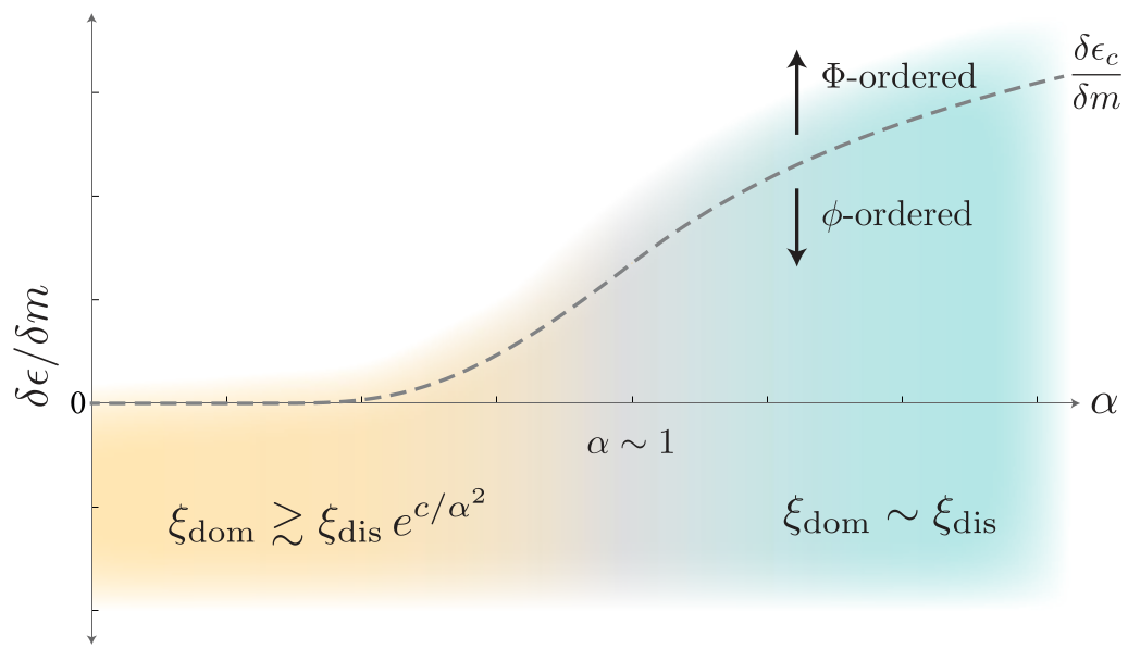
So far in this section, the QVH insulator has been taken as the true ground state of mTBG at charge neutrality, even in the absence of disorder. We now address the possibility that interactions prefer a different state. To simplify the problem, we consider the situation in which a single competing phase is energetically favourable relative to the QVH insulator. In accordance with the conventions of Sec. V.1, this competition can be quantified through the energy difference $\delta\epsilon$ in an area of size $\ell_{\mathrm{UV}}^{2}=\xi_{\mathrm{int}}^{2}$:

where $\mathcald{E}_{\mathrm{QVH}}$ and $\mathcald{E}_{\mathrm{C}}$ respectively denote the ground-state energy densities of the QVH state and competing phase. We further assume that the competing order may be described by an Ising field, $\Phi$, that does not linearly couple to any disorder field; recall the discussion at the end of Sec. IV.3. Generalizing our arguments to include continuous order parameters (as needed for the QSH and QSVH insulators) is straightforward, and we therefore leave the competing phase’s identity unspecified.

We again work in a regime where strong interactions obviate the need to include all disorder fields save for the random mass $\mathcal{M}_{0}$ that linearly couples to the QVH order parameter via Eq. (17). Importantly, this type of disorder locally promotes the QVH state by lowering its energy relative to the competing phase, even though—as we saw earlier—it generally destroys true long-range order. When $\delta\epsilon$ is small enough, we expect the majority of the sample to realize the QVH phase and the scenario outlined in the previous section to hold. In terms of the Ising theory devised in the previous section, we can express this condition as

where ‘$\mathrm{vol}$’ denotes the sample volume. When this equation holds, we say the system is ‘$\phi$-ordered’; otherwise, the system is ‘$\Phi$-ordered.’

Appendix F explores this problem in depth, ultimately deriving the schematic phase diagram shown in Fig. 5. We again find that the primary control parameter is the ratio $\alpha$ [recall Eq. (18)] corresponding to the horizontal axis. Motivated by the notion that $\Phi$-ordered regions may be viewed as annealed ‘vacancies,’ we begin with a dilute Ising-model description. At the lattice level, the theory is conveniently formulated by promoting the Ising variables $\sigma^{z}=\pm 1$ to three-state spin-1 variables $s$, where $s=\pm 1$ correspond to the two QVH phases and $s=0$ corresponds to the competing phase. We present a simple mean-field solution to the classical Blume-Capel model for these spin-1 degrees of freedom Blume 1966; Capel 1966; Kaufman and Kanner 1990; Vasseur and Lookman 2010 in Appendix F.1. While the phase diagram we obtain resembles the one shown in Fig. 5 in many respects, it erroneously predicts long-range $\phi$-order when $\delta\epsilon<0$ and disorder is sufficiently small, $\alpha\lesssim 1$; as discussed in Sec. V.1 and Appendix E, in reality, long-range order is unstable to the addition of any finite disorder. This failure of mean-field theory is not unprecedented given the low dimensionality.

In Appendix F.2, we therefore return to the Imry-Ma type arguments of Sec. V.1 (see also Appendix E), which allow us to derive a ‘critical’ energy difference $\delta\epsilon_{c}(\alpha)$ that characterizes the crossover scale separating $\phi$- and $\Phi$-ordered regimes. We plot $\delta\epsilon_{c}(\alpha)$ with a dashed line in Fig. 5. In the white region above the line, $\delta\epsilon\gtrsim\delta\epsilon_{c}(\alpha)$, the competing phase is realized throughout the majority of the system, and the network picture we propose is no longer relevant. Conversely, Eq. (22) holds in regions where $\delta\epsilon\lesssim\delta\epsilon_{c}(\alpha)$ (including the trivial case, $\delta\epsilon<0$, where QVH states minimize the energy in the clean limit). Just as we found above, depending on the strength of disorder, the destruction of long-range QVH order occurs in two fashions. In Fig. 5, the parameter regime where $\Braket{\phi}$ tracks the disorder field is shown in turquoise. The orange area indicates the opposite limit, where long-range order is eliminated by domain-wall condensation. The intermediate regime where $\alpha\sim 1$ is shown in neutral grey.

Notably, these considerations imply that disorder may not only be responsible for selecting which QVH order is locally realized, but that it may also determine whether or not QVH order is realized at all. In particular, our proposal admits a scenario in which the clean samples of Lu et al. Lu et al. 2019 are $\Phi$-ordered, while the less homogeneous samples of Cao et al. Cao et al. 2018a; Cao et al. 2018b and Yankowitz et al. Yankowitz et al. 2019 realize the QVH network picture displayed in the central panel of Fig. 2—even supposing that the two sets of systems differ solely in the amount of disorder they present.

In the absence of any special symmetries, all two-dimensional systems are generically expected to localize in the thermodynamic limit, and our platform is no exception. Localization is likely irrelevant for the previously studied mTBG samples, whose linear dimensions are $\sim 2-8\,\mathrm{\mu\text{m}}\sim 150-600a_{\hskip-0.40974ptM}$. It is nevertheless instructive to briefly discuss localization within our proposed scenario. The precise manner in which localization occurs in the presence of interactions poses a notoriously difficult and subtle problem that we will not wade into in detail. Rather, our goal is to discuss some general features of the problem that can be deduced given some reasonable simplifying assumptions.

When discussing localization, one can imagine either increasing the system size or increasing the disorder strength. In the latter case, the situation rapidly becomes unwieldy: as the disorder strength approaches the interaction energy ($\delta m/U\to 1$) or the disorder correlations become ultra-short-ranged ($a_{\hskip-0.40974ptM}/\xi_{\mathrm{dis}}\to 1$), our Ising formulation breaks down. By contrast, the Ising-model perspective remains valid when we instead consider progressively larger samples with an otherwise identical set of parameters. Interactions can still of course pose complications; for instance, in the network-model picture localization involves a network of gapless domain-wall modes that generically form Luttinger liquids Chou et al. 2019. We do not address such subtleties, instead postulating that the primary effect of interactions is to catalyze the spontaneous breaking of ${\mathcald{C}}_{2}{\mathcald{T}}$.

The most straightforward manner by which the re-emergent Dirac fermions can localize is through inter-${\boldsymbol{\kappa}}$-valley scattering. Such scattering events can also localize the original Dirac cones that appear in the free-fermion band structure for mTBG, but the physics is not quite identical: the network picture underlying the re-emergent Dirac cones effectively postpones localization by renormalizing the UV scale at which it occurs. That is, if $\xi_{\mathrm{loc},\mathit{fr}}$ is the localization length in the free case, we have $\xi_{\mathrm{loc}}\sim\xi_{\mathrm{dom}}\xi_{\mathrm{loc},\mathit{fr}}/a_{\hskip-0.40974ptM}$ with interactions. One can intuitively understand this rescaling from the perspective of the gapless domain-wall modes in the network model. As Fig. 6 illustrates, in a given ${\boldsymbol{K}}$-valley, the domain-wall modes corresponding to $\pm{\boldsymbol{\kappa}}$ co-propagate, and hence non-forward-scattering processs can only occur at nodes where multiple domain walls intersect (see red arrows).

Inter-${\boldsymbol{K}}$-valley scattering can also prompt localization Qiao et al. 2011. Disorder coupling the two ${\boldsymbol{K}}$-valleys has so far been completely ignored since it is exponentially suppressed relative to intra-${\boldsymbol{\kappa}}$-scattering [see Eq. (8)]. However, inter-${\boldsymbol{K}}$-valley scattering can occur at any point along the domain walls, as illustrated in Fig. 6, making it a fundamentally one-dimensional process. For very large domains, such intra-domain-wall scattering thus inevitably becomes the dominant localization mechanism. The localization length is then expected to be proportional to the mean free path of the domain-wall modes Evers and Mirlin 2008, which is $\xi_{\mathrm{loc}}\sim\hbar v_{F}/g_{\mathit{KK^{\prime}}}\sim\hbar v_{F}e^{4\pi^{2}\xi_{\mathrm{dis}}^{2}/a^{2}}/g$, and hence an exponentially large function of the disorder correlation length.

References

- Cao et al. (2018a) Y. Cao, V. Fatemi, S. Fang, K. Watanabe, T. Taniguchi, E. Kaxiras, and P. Jarillo-Herrero, Nature (London) 556, 43 (2018a), arXiv:1803.02342 [cond-mat.mes-hall] .
- Cao et al. (2018b) Y. Cao, V. Fatemi, A. Demir, S. Fang, S. L. Tomarken, J. Y. Luo, J. D. Sanchez-Yamagishi, K. Watanabe, T. Taniguchi, E. Kaxiras, R. C. Ashoori, and P. Jarillo-Herrero, Nature (London) 556, 80 (2018b), arXiv:1802.00553 [cond-mat.mes-hall] .
- Lopes Dos Santos et al. (2007) J. M. B. Lopes Dos Santos, N. M. R. Peres, and A. H. Castro Neto, Phys. Rev. Lett. 99, 256802 (2007), arXiv:0704.2128 [cond-mat.mtrl-sci] .
- Bistritzer and MacDonald (2011) R. Bistritzer and A. H. MacDonald, Proceedings of the National Academy of Science 108, 12233 (2011), arXiv:1009.4203 [cond-mat.mes-hall] .
- Kim et al. (2015) Y. Kim, B. J. Wieder, C. L. Kane, and A. M. Rappe, Phys. Rev. Lett. 115, 036806 (2015), arXiv:1504.03807 [cond-mat.mtrl-sci] .
- Po et al. (2018) H. C. Po, L. Zou, A. Vishwanath, and T. Senthil, Physical Review X 8, 031089 (2018), arXiv:1803.09742 [cond-mat.str-el] .
- de Gail et al. (2011) R. de Gail, M. O. Goerbig, F. Guinea, G. Montambaux, and A. H. Castro Neto, Phys. Rev. B 84, 045436 (2011), arXiv:1103.3172 [cond-mat.mes-hall] .
- He et al. (2013) W.-Y. He, Z.-D. Chu, and L. He, Phys. Rev. Lett. 111, 066803 (2013), arXiv:1301.7573 [cond-mat.mes-hall] .
- Yankowitz et al. (2019) M. Yankowitz, S. Chen, H. Polshyn, Y. Zhang, K. Watanabe, T. Taniguchi, D. Graf, A. F. Young, and C. R. Dean, Science 363, 1059 (2019), arXiv:1808.07865 [cond-mat.mes-hall] .
- Sharpe et al. (2019) A. L. Sharpe, E. J. Fox, A. W. Barnard, J. Finney, K. Watanabe, T. Taniguchi, M. A. Kastner, and D. Goldhaber-Gordon, Science 365, 605 (2019), arXiv:1901.03520 [cond-mat.mes-hall] .
- Serlin et al. (2019) M. Serlin, C. L. Tschirhart, H. Polshyn, Y. Zhang, J. Zhu, K. Watanabe, T. Taniguchi, L. Balents, and A. F. Young, (2019), arXiv:1907.00261 [cond-mat.str-el] .
- Bultinck et al. (2019a) N. Bultinck, S. Chatterjee, and M. P. Zaletel, arXiv:1901.08110 [cond-mat.str-el] (2019a).
- Zhang et al. (2019a) Y.-H. Zhang, D. Mao, and T. Senthil, arXiv:1901.08209 [cond-mat.str-el] (2019a).
- Lu et al. (2019) X. Lu, P. Stepanov, W. Yang, M. Xie, M. A. Aamir, I. Das, C. Urgell, K. Watanabe, T. Taniguchi, G. Zhang, A. Bachtold, A. H. MacDonald, and D. K. Efetov, arXiv:1903.06513 [cond-mat.str-el] (2019).
- Kerelsky et al. (2019) A. Kerelsky, L. J. McGilly, D. M. Kennes, L. Xian, M. Yankowitz, S. Chen, K. Watanabe, T. Taniguchi, J. Hone, C. Dean, A. Rubio, and A. N. Pasupathy, Nature 572, 95 (2019), arXiv:1812.08776 [cond-mat.mes-hall] .
- Choi et al. (2019) Y. Choi, J. Kemmer, Y. Peng, A. Thomson, H. Arora, R. Polski, Y. Zhang, H. Ren, J. Alicea, G. Refael, F. von Oppen, K. Watanabe, T. Taniguchi, and S. Nadj-Perge, Nature Physics 10.1038/s41567-019-0606-5 (2019), arXiv:1901.02997 [cond-mat.mes-hall] .
- Jiang et al. (2019) Y. Jiang, X. Lai, K. Watanabe, T. Taniguchi, K. Haule, J. Mao, and E. Y. Andrei, Nature 573, 91 (2019), arXiv:1904.10153 [cond-mat.mes-hall] .
- Xie et al. (2019) Y. Xie, B. Lian, B. Jäck, X. Liu, C.-L. Chiu, K. Watanabe, T. Taniguchi, B. A. Bernevig, and A. Yazdani, Nature 572, 101 (2019), arXiv:1906.09274 [cond-mat.mes-hall] .
- Uri et al. (2019) A. Uri, S. Grover, Y. Cao, J. A. Crosse, K. Bagani, D. Rodan-Legrain, Y. Myasoedov, K. Watanabe, T. Taniguchi, P. Moon, M. Koshino, P. Jarillo-Herrero, and E. Zeldov, arXiv:1908.04595 [cond-mat.mes-hall] (2019).
- Wilson et al. (2019) J. H. Wilson, Y. Fu, S. Das Sarma, and J. H. Pixley, 1908.02753 [cond-mat.dis-nn] (2019).
- Liu et al. (2019) S. Liu, E. Khalaf, J. Y. Lee, and A. Vishwanath, (2019), arXiv:1905.07409 [cond-mat.str-el] .
- Xie and MacDonald (2018) M. Xie and A. H. MacDonald, arXiv:1812.04213 [cond-mat.str-el] (2018).
- Zhang et al. (2011) F. Zhang, J. Jung, G. A. Fiete, Q. Niu, and A. H. MacDonald, Phys. Rev. Lett. 106, 156801 (2011), arXiv:1010.4003 [cond-mat.str-el] .
- Martin et al. (2008) I. Martin, Y. M. Blanter, and A. F. Morpurgo, Phys. Rev. Lett. 100, 036804 (2008), arXiv:0709.3522 [cond-mat.mes-hall] .
- Qiao et al. (2011) Z. Qiao, J. Jung, Q. Niu, and A. H. MacDonald, Nano Letters 11, 3453 (2011), arXiv:1107.4550 [cond-mat.mes-hall] .
- Yin et al. (2016) L.-J. Yin, H. Jiang, J.-B. Qiao, and L. He, Nature Communications 7, 11760 (2016), arXiv:1511.06498 [cond-mat.mes-hall] .
- Ju et al. (2015) L. Ju, Z. Shi, N. Nair, Y. Lv, C. Jin, J. Velasco, C. Ojeda-Aristizabal, H. A. Bechtel, M. C. Martin, A. Zettl, J. Analytis, and F. Wang, Nature (London) 520, 650 (2015).
- Li et al. (2016) J. Li, K. Wang, K. J. McFaul, Z. Zern, Y. Ren, K. Watanabe, T. Taniguchi, Z. Qiao, and J. Zhu, Nature Nanotechnology 11, 1060 (2016), arXiv:1509.03912 [cond-mat.mes-hall] .
- Abanin et al. (2010) D. A. Abanin, S. A. Parameswaran, S. A. Kivelson, and S. L. Sondhi, Phys. Rev. B 82, 035428 (2010), arXiv:1003.1978 [cond-mat.mes-hall] .
- Parameswaran and Feldman (2019) S. A. Parameswaran and B. E. Feldman, Journal of Physics Condensed Matter 31, 273001 (2019), arXiv:1809.09616 [cond-mat.str-el] .
- Mross et al. (2018) D. F. Mross, Y. Oreg, A. Stern, G. Margalit, and M. Heiblum, Phys. Rev. Lett. 121, 026801 (2018).
- Wang et al. (2018) C. Wang, A. Vishwanath, and B. I. Halperin, Phys. Rev. B 98, 045112 (2018).
- Lian and Wang (2018) B. Lian and J. Wang, Phys. Rev. B 97, 165124 (2018).
- Chalker and Coddington (1988) J. T. Chalker and P. D. Coddington, Journal of Physics C: Solid State Physics 21, 2665 (1988).
- Lee and Chalker (1994) D. K. K. Lee and J. T. Chalker, Phys. Rev. Lett. 72, 1510 (1994), arXiv:cond-mat/9311050 [cond-mat] .
- Lee et al. (1994) D. K. K. Lee, J. T. Chalker, and D. Y. K. Ko, Phys. Rev. B 50, 5272 (1994).
- Ho and Chalker (1996) C. M. Ho and J. T. Chalker, Physical Review B 54, 8708 (1996), arXiv:cond-mat/9605073 [cond-mat] .
- Lee (1994) D.-H. Lee, Phys. Rev. B 50, 10788 (1994), cond-mat/9404011 [cond-mat] .
- Nam and Koshino (2017) N. N. T. Nam and M. Koshino, Phys. Rev. B 96, 075311 (2017), arXiv:1706.03908 [cond-mat.mtrl-sci] .
- Koshino et al. (2018) M. Koshino, N. F. Q. Yuan, T. Koretsune, M. Ochi, K. Kuroki, and L. Fu, Physical Review X 8, 031087 (2018), arXiv:1805.06819 [cond-mat.mes-hall] .
- Po et al. (2019) H. C. Po, L. Zou, T. Senthil, and A. Vishwanath, Phys. Rev. B 99, 195455 (2019), arXiv:1808.02482 [cond-mat.str-el] .
- Kang and Vafek (2018) J. Kang and O. Vafek, Physical Review X 8, 031088 (2018), arXiv:1805.04918 [cond-mat.str-el] .
- Zou et al. (2018) L. Zou, H. C. Po, A. Vishwanath, and T. Senthil, Physical Review B 98, 085435 (2018), arXiv:1806.07873 [cond-mat.str-el] .
- Zirnbauer (1996) M. R. Zirnbauer, Journal of Mathematical Physics 37, 4986 (1996), arXiv:math-ph/9808012 [math-ph] .
- Altland and Zirnbauer (1997) A. Altland and M. R. Zirnbauer, Phys. Rev. B 55, 1142 (1997), arXiv:cond-mat/9602137 [cond-mat] .
- Ludwig et al. (1994) A. W. W. Ludwig, M. P. A. Fisher, R. Shankar, and G. Grinstein, Phys. Rev. B 50, 7526 (1994).
- Ostrovsky et al. (2007) P. M. Ostrovsky, I. V. Gornyi, and A. D. Mirlin, Phys. Rev. Lett. 98, 256801 (2007), arXiv:cond-mat/0702115 [cond-mat.mes-hall] .
- Morpurgo and Guinea (2006) A. F. Morpurgo and F. Guinea, Phys. Rev. Lett. 97, 196804 (2006), arXiv:cond-mat/0603789 [cond-mat.mes-hall] .
- Pruisken (1984) A. Pruisken, Nuclear Physics B 235, 277 (1984).
- Pruisken (1990) A. M. M. Pruisken, Field theory, scaling and the localization problem, in The Quantum Hall Effect, edited by R. E. Prange and S. M. Girvin (Springer New York, New York, NY, 1990) pp. 117–173.
- Aleiner and Efetov (2006) I. L. Aleiner and K. B. Efetov, Phys. Rev. Lett. 97, 236801 (2006), arXiv:cond-mat/0607200 [cond-mat.dis-nn] .
- Altland (2006) A. Altland, Phys. Rev. Lett. 97, 236802 (2006), arXiv:cond-mat/0607247 [cond-mat.mes-hall] .
- Abrahams et al. (1979) E. Abrahams, P. W. Anderson, D. C. Licciardello, and T. V. Ramakrishnan, Phys. Rev. Lett. 42, 673 (1979).
- Lee and Ramakrishnan (1985) P. A. Lee and T. V. Ramakrishnan, Rev. Mod. Phys. 57, 287 (1985).
- Fradkin (1986a) E. Fradkin, Phys. Rev. B 33, 3257 (1986a).
- Fradkin (1986b) E. Fradkin, Phys. Rev. B 33, 3263 (1986b).
- Carr et al. (2019) S. Carr, S. Fang, Z. Zhu, and E. Kaxiras, Phys. Rev. Research 1, 013001 (2019), arXiv:1901.03420 [cond-mat.mes-hall] .
- Haldane (1988) F. D. M. Haldane, Phys. Rev. Lett. 61, 2015 (1988).
- Weeks and Franz (2010) C. Weeks and M. Franz, Phys. Rev. B 81, 085105 (2010).
- Kane and Mele (2005) C. L. Kane and E. J. Mele, Phys. Rev. Lett. 95, 226801 (2005).
- Tarnopolsky et al. (2019) G. Tarnopolsky, A. J. Kruchkov, and A. Vishwanath, Phys. Rev. Lett. 122, 106405 (2019), arXiv:1808.05250 [cond-mat.str-el] .
- Zhang et al. (2019b) Y.-H. Zhang, D. Mao, Y. Cao, P. Jarillo-Herrero, and T. Senthil, Phys. Rev. B 99, 075127 (2019b), arXiv:1805.08232 [cond-mat.str-el] .
- Lee et al. (2019) J. Y. Lee, E. Khalaf, S. Liu, X. Liu, Z. Hao, P. Kim, and A. Vishwanath, arXiv:1903.08685 [cond-mat.str-el] (2019).
- Bultinck et al. (2019b) N. Bultinck, E. Khalaf, S. Liu, S. Chatterjee, A. Vishwanath, and M. P. Zaletel, , arXiv:1911.02045 (2019b), arXiv:1911.02045 [cond-mat.str-el] .
- Dotsenko and Dotsenko (1983) V. S. Dotsenko and V. S. Dotsenko, Advances in Physics 32, 129 (1983).
- Imry and Ma (1975) Y. Imry and S.-k. Ma, Phys. Rev. Lett. 35, 1399 (1975).
- Nattermann and Villain (1988) T. Nattermann and J. Villain, Phase Transitions 11, 5 (1988).
- Nattermann (1997) T. Nattermann, Spin Glasses And Random Fields. Series: Series on Directions in Condensed Matter Physics 12, 277 (1997), arXiv:cond-mat/9705295 [cond-mat.stat-mech] .
- Binder (1983) K. Binder, Zeitschrift für Physik B Condensed Matter 50, 343 (1983).
- Aizenman and Wehr (1989) M. Aizenman and J. Wehr, Phys. Rev. Lett. 62, 2503 (1989).
- Blume (1966) M. Blume, Phys. Rev. 141, 517 (1966).
- Capel (1966) H. Capel, Physica 32, 966 (1966).
- Kaufman and Kanner (1990) M. Kaufman and M. Kanner, Phys. Rev. B 42, 2378 (1990).
- Vasseur and Lookman (2010) R. Vasseur and T. Lookman, Phys. Rev. B 81, 094107 (2010).
- Chou et al. (2019) Y.-Z. Chou, R. M. Nandkishore, and L. Radzihovsky, Phys. Rev. B 99, 165108 (2019), arXiv:1901.05464 [cond-mat.str-el] .
- Evers and Mirlin (2008) F. Evers and A. D. Mirlin, Reviews of Modern Physics 80, 1355 (2008), arXiv:0707.4378 [cond-mat.mes-hall] .
- Efimkin and MacDonald (2018) D. K. Efimkin and A. H. MacDonald, Phys. Rev. B 98, 035404 (2018), arXiv:1803.06404 [cond-mat.mes-hall] .
- Wu et al. (2019) X.-C. Wu, C.-M. Jian, and C. Xu, Phys. Rev. B 99, 161405 (2019), arXiv:1811.08442 [cond-mat.str-el] .
- Woods et al. (2014) C. R. Woods, L. Britnell, A. Eckmann, R. S. Ma, J. C. Lu, H. M. Guo, X. Lin, G. L. Yu, Y. Cao, R. V. Gorbachev, A. V. Kretinin, J. Park, L. A. Ponomarenko, M. I. Katsnelson, Y. N. Gornostyrev, K. Watanabe, T. Taniguchi, C. Casiraghi, H. J. Gao, A. K. Geim, and K. S. Novoselov, Nature Physics 10, 451 (2014), arXiv:1401.2637 [cond-mat.mes-hall] .
- van Wijk et al. (2015) M. M. van Wijk, A. Schuring, M. I. Katsnelson, and A. Fasolino, 2D Materials 2, 034010 (2015), arXiv:1503.02540 [cond-mat.mes-hall] .
- Dai et al. (2016) S. Dai, Y. Xiang, and D. J. Srolovitz, Nano Letters 16, 5923 (2016).
- Kim et al. (2017) N. Y. Kim, H. Y. Jeong, J. H. Kim, G. Kim, H. S. Shin, and Z. Lee, ACS Nano 11, 7084 (2017).
- Gargiulo and Yazyev (2018) F. Gargiulo and O. V. Yazyev, 2D Materials 5, 015019 (2018), arXiv:1711.08647 [cond-mat.mes-hall] .
- Zhang and Tadmor (2018) K. Zhang and E. B. Tadmor, Journal of Mechanics Physics of Solids 112, 225 (2018).
- (85) We thank Cory Dean for sharing these ideas with us.
- Hofstadter (1976) D. R. Hofstadter, Phys. Rev. B 14, 2239 (1976).
- Tworzydło et al. (2006) J. Tworzydło, B. Trauzettel, M. Titov, A. Rycerz, and C. W. J. Beenakker, Phys. Rev. Lett. 96, 246802 (2006), arXiv:cond-mat/0603315 [cond-mat.mes-hall] .
- Peres et al. (2006) N. M. R. Peres, A. H. Castro Neto, and F. Guinea, Phys. Rev. B 73, 195411 (2006), arXiv:cond-mat/0512476 [cond-mat.mes-hall] .
- Das Sarma et al. (2011) S. Das Sarma, S. Adam, E. H. Hwang, and E. Rossi, Reviews of Modern Physics 83, 407 (2011), arXiv:1003.4731 [cond-mat.mes-hall] .
- Ando (2006) T. Ando, Journal of the Physical Society of Japan 75, 074716 (2006).
- Cheianov and Fal’Ko (2006) V. V. Cheianov and V. I. Fal’Ko, Phys. Rev. Lett. 97, 226801 (2006), arXiv:cond-mat/0608228 [cond-mat.mes-hall] .
- Nomura and MacDonald (2006) K. Nomura and A. H. MacDonald, Phys. Rev. Lett. 96, 256602 (2006), arXiv:cond-mat/0604113 [cond-mat.mes-hall] .
- Hwang et al. (2007) E. H. Hwang, S. Adam, and S. D. Sarma, Phys. Rev. Lett. 98, 186806 (2007), arXiv:cond-mat/0610157 [cond-mat.mes-hall] .
- Nomura and MacDonald (2007) K. Nomura and A. H. MacDonald, Phys. Rev. Lett. 98, 076602 (2007), arXiv:cond-mat/0606589 [cond-mat.mes-hall] .
- Trushin and Schliemann (2008) M. Trushin and J. Schliemann, EPL (Europhysics Letters) 83, 17001 (2008), arXiv:0802.2794 [cond-mat.mes-hall] .
- Katsnelson et al. (2009) M. I. Katsnelson, F. Guinea, and A. K. Geim, arXiv e-prints , arXiv:0901.1398 (2009), arXiv:0901.1398 [cond-mat.mes-hall] .
- Katsnelson and Geim (2008) M. I. Katsnelson and A. K. Geim, Philosophical Transactions of the Royal Society of London Series A 366, 195 (2008), arXiv:0706.2490 [cond-mat.mes-hall] .
- Nattermann (1983) T. Nattermann, Journal of Physics C: Solid State Physics 16, 6407 (1983).
- Seppälä et al. (1998) E. T. Seppälä, V. Petäjä, and M. J. Alava, Phys. Rev. E 58, R5217 (1998).
- Seppälä and Alava (2001) E. T. Seppälä and M. J. Alava, Physical Review E 63, 10.1103/physreve.63.066109 (2001).