A dynamic programming approach to solving constrained linear-quadratic optimal control problems

For any $M\in\mathbb{R}^{a\times b}$ and any ordered set $\mathcal{M}\subseteq\{1,...,a\}$ let $M_{\mathcal{M}}\in\mathbb{R}^{|\mathcal{M}|\times b}$ be the submatrix of $M$ containing all rows indicated by $\mathcal{M}$. Let $\oplus$ and $\ominus$ denote the Minkowski addition and Pontryagin difference, respectively.

Let $\mathcal{P}(\mathcal{Q})$ refer to the power set of $\mathcal{Q}$ and note that the set of active sets $\mathcal{M}_{N}$ that define the solution is a subset of $\mathcal{P}(\mathcal{Q})$. It is the basic idea of combinatorial quadratic programming to efficiently determine those $\mathcal{A}\in\mathcal{P}(\mathcal{Q})$ that make up $\mathcal{M}_{N}$.

All $\mathcal{A}\in\mathcal{M}_{N}$ are optimal active sets by definition of $\mathcal{M}_{N}$. For clarity, we call any $\mathcal{A}\in\mathcal{P}(\mathcal{Q})$ that is not known to be optimal a candidate active set. A candidate $\mathcal{A}\in\mathcal{P}(\mathcal{Q})$ is optimal, if the linear program (LP)

has a solution [6, Sect. 3.1], where $e_{i}=(1\cdots 1)^{T}$, $i=1,2$ are column vectors of appropriate sizes, $\lambda_{\mathcal{A}}$ are Lagrangian multipliers and $s_{\mathcal{I}}$ are slack variables. Furthermore, we follow [6] in calling an $\mathcal{A}\in\mathcal{P}(\mathcal{Q})$ feasible (resp. infeasible), if (8) without (8b) and (8c) has a solution (resp. has no solution). Since this smaller LP involves a subset of the constraints of (8), feasibility of $\mathcal{A}$ is a necessary condition for optimality of $\mathcal{A}$, or equivalently, an $\mathcal{A}$ that is infeasible is not optimal. The LP without (8b) and (8c) is particularly useful, because it typically permits to disregard many candidates $\mathcal{A}\in\mathcal{P}(\mathcal{Q})$ after solving only one LP. Specifically, if $\mathcal{A}\in\mathcal{P}(\mathcal{Q})$ is infeasible, then additional active constraints cannot result in feasibility and therefore every $\mathcal{A}^{\prime}\supset\mathcal{A}$ is also infeasible [6, Thm. 1].

An optimal active set $\mathcal{A}$ defines a full-dimensional polytope, if $G_{\mathcal{A}}$ is of full row rank and if both $G_{\mathcal{I}}U<w_{\mathcal{I}}+E_{\mathcal{I}}x(0)$ and $\lambda_{\mathcal{A}}>0$ hold [18, Thm. 2]. Full-dimensional polytopes defined by active sets such that $G_{\mathcal{A}}$ does not have full row rank are not required, because their polytopes are covered by the polytopes defined by the active sets in $\mathcal{M}_{N}$ [1, Sect. 3].

Algorithm 1 from [6] serves as a reference to which the approach proposed here is compared. In contrast to the new algorithm stated in Sect. 3, Alg. 1 only considers candidates $\mathcal{A}$ such that $G_{\mathcal{A}}$ has full rank. Since $G_{\mathcal{A}}\in\mathbb{R}^{|\mathcal{A}|\times mN}$, the row rank of $G_{\mathcal{A}}$ is bounded from above by $\min(|A|,mN)$. Consequently, $G_{\mathcal{A}}$ does not have full row rank if $|A|>mN$ and only the candidates $\mathcal{A}\in\mathcal{P}^{\prime}(\mathcal{Q})=\{\mathcal{A}\in\mathcal{P}(\mathcal{Q})||\mathcal{A}|\leq mN\}$ need to be considered (line 2 in Alg. 1). The solution $t=0$ to (8) indicates that either $G_{\{i\}}U=w_{\{i\}}+E_{\{i\}}x(0)$ holds for an $i\in\mathcal{I}$ or $\lambda_{\{j\}}=0$ holds for a $j\in\mathcal{A}$. In this case the active set is only added to $\mathcal{M}_{N}$ if the polytope defined by $\mathcal{A}$ (see e.g. [10, Lem. 2]) is full-dimensional.

Assuming the set $S_{N}$ is known for some horizon $N$, the set $S_{N+1}$ can be determined with Alg. 2, which essentially implements Cor. 3. Specifically, lines 4,5 correspond to (13a) and lines 8,9 correspond to (13b) in Cor. 3.

Candidate active sets are tested for optimality for the OCP with horizon $N+1$, unless they can be disregarded because they are supersets of a known infeasible active set (line 10). Candidate active sets are added to $\mathcal{S}_{N+1}$ if they are optimal (lines 12,13) and tested for feasibility otherwise (line 17). Sets known to be infeasible are stored (lines 18,19) in order to be able to quickly dismiss supersets that appear later. The set $\mathcal{S}_{N}^{\rm degen.}$ collects all $\mathcal{A}\in\mathcal{S}_{N}$ such that the solution to (8) is $t=0$. $\mathcal{S}_{N+1}^{\rm degen.}$ is then determined by collecting all $\mathcal{A}\in\mathcal{S}_{N}^{\rm degen.}$ that were copied with (13a) (lines 6,7) and all candidate active sets such that the solution to (8) is $t=0$ (lines 14,15). Since active sets that are infeasible for horizon $N$ are not necessarily infeasible for horizon $N+1$, $\mathcal{S}_{N+1}^{\rm pruned}$ is initialized with the empty set in line 2.

The initial sets $\mathcal{S}_{1}$ and $\mathcal{S}_{1}^{\rm degen.}$ can be determined with Alg. 3, which proceeds analogously to Alg. 1 but does not discard candidate active sets such that $G_{\mathcal{A}}$ is not of full rank. In case the solution to (8) is $t=0$, the candidate active set is added to both $\mathcal{S}_{1}$ and $\mathcal{S}_{1}^{\rm degen.}$.

The overall dynamic programming approach is stated in Alg. 4. The algorithm terminates if the desired horizon $N_{\rm max}$ has been reached or if an $N$ such that $\mathcal{F}_{\infty}=\mathcal{F}_{N}$ has been found with Prop. 4. The condition in line 5 of Alg. 4 merely is a compact way of stating that all active sets in $\mathcal{S}_{N+1}$ have no active constraints in stages $N$ and $N+1$ and thus is equivalent to $\tilde{\mathcal{S}}_{N+1}=\emptyset$. Lines 8-14 in Alg. 4 reduce $\mathcal{S}_{N}$ to $\mathcal{M}_{N}\subseteq\mathcal{S}_{N}$ by discarding all active sets such that $G_{\mathcal{A}}$ does not have full rank and by testing all active sets that are element of $\mathcal{S}_{N}^{\rm degen.}$ for defining a full-dimensional polytope.

In contrast to Alg. 1, Alg. 4 does not consider all $\mathcal{A}\in\mathcal{P}^{\prime}(\mathcal{Q})$, but it generates candidate active sets with Cor. 3, thus reducing their number. On the other hand, candidate active sets such that $G_{\mathcal{A}}$ is not of full rank are discarded in Alg. 1, but not in Alg. 4. In fact, an $\mathcal{A}_{i}\in\mathcal{S}_{N+1}$ such that $G_{\mathcal{A}i}$ is of full rank may result with (9) from a $\mathcal{A}_{l}\in\mathcal{S}_{N}$ such that $G_{\mathcal{A}l}$ is not of full rank This is illustrated in Fig. 1. The results in Sect. 4.2 show that considerable overall savings result with the method proposed here even though active sets such that $G_{\mathcal{A}}$ is not of full rank are no longer discarded.

Figures 2 and 3 show solutions for the OCP (2) as a function of the horizon. Gray polytopes correspond to active sets with at least one active terminal constraint. Blue polytopes correspond to active sets with no active terminal constraints (stage $N$) but at least one active constraint in stage $N-1$. White polytopes correspond to active sets with no active constraints in stages $N-1$ and $N$. The set $\mathcal{S}_{N}$ contains the active sets of all shown polytopes. $\tilde{\mathcal{S}}_{N}$ as defined in (14) contains the active sets of all blue and gray polytopes.

Figure 2 illustrates Cor. 3 with the solutions for $N=2$ and $N=3$. All elements in $\mathcal{S}_{2}$ with no active terminal constraints (blue and white polytopes) also appear in the solution for the increased horizon $\mathcal{S}_{3}$. For example, $\mathcal{A}_{1}$ and $\mathcal{A}_{2}$ exists for both $N=2$ and $N=3$ according to Lem. 2 and (13a). All elements in $\tilde{\mathcal{S}}_{2}$ (blue and gray polytopes) are the basis for the generation of candidate active sets for $\mathcal{S}_{3}$ according to (13b) in Cor. 3. For example, the blue polytopes with active sets $\mathcal{A}_{2a},...,\mathcal{A}_{2c}$ in $\mathcal{S}_{3}$ result with (13b) from $\mathcal{A}_{2}$, and the gray polytope $\mathcal{A}_{3a}$ results with (13b) from $\mathcal{A}_{3}$.

Proposition 4 states the solution will not change for horizons $\tilde{N}>N$, if $\tilde{\mathcal{S}}_{N}=\emptyset$. The horizon $N=16$ is the shortest horizon such that $\tilde{\mathcal{S}}_{N}=\emptyset$. The resulting solution set $\mathcal{F}_{\infty}=\mathcal{F}_{16}$ is shown in Fig. 3. All polytopes belong to active sets with no active constraints in stages $N-1$ and $N$ (i.e., white polytopes) as expected. We note that $\mathcal{F}_{\infty}=\mathcal{F}_{15}$ holds, since all active sets in $\mathcal{M}_{15}$, where $\mathcal{M}_{15}$ results from Alg. 4, have no active terminal constraints [12, Prop. 6].

Figure 4 compares the computational costs of the existing approach (Alg. 1) and the approach proposed here (Alg. 4). The figure shows the numbers of generated candidate active sets, pruning tests, rank tests, optimality tests with (8), and feasibility tests with (8) without (8b) and (8c) for both algorithms. In Alg. 1, the number of generated candidate active sets equals the cardinality of $\mathcal{P}^{\prime}(\mathcal{Q})$. In Alg. 4, the number of generated candidate active sets is equal to the sum of the cardinalities of $\mathcal{P}(\{1,...,q_{\mathcal{UX}}+q_{\mathcal{T}}\})$ and all $\mathcal{R}^{(2)}$ for horizons $N=1,...,N_{\max}-1$.

All curves in Fig. 4 intersect for small values of $N$, which implies Alg. 1 outperforms Alg. 4 for small $N$. The point of intersection is enlarged in Fig. 5. For larger $N$, Alg. 4 is more efficient than Alg. 1 and it is evident from Fig. 4 this difference gets more pronounced as $N$ increases.

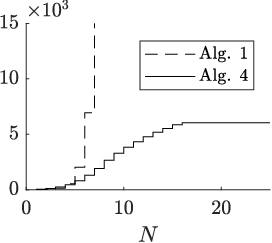
Algorithms 1 and 4 mainly differ with respect to the fundamentally different procedures for generating candidate active sets. This difference becomes evident in Fig. 4(a). Most importantly, a plateau results for Alg. 4 in Fig. 4 because $\mathcal{F}_{\infty}=\mathcal{F}_{15}$. Since fewer candidate active sets entail fewer rank, pruning, optimality and feasibility tests, the qualitative difference of the curves in Fig. 4(a) is inherited by the remaining curves.

In both algorithms, the optimality tests with LP (8) only need to be carried out for a subset of the candidate active sets (compare Figs. 4(a) and 4(d)). In Alg. 1, candidates can be dismissed because they are supersets of known infeasible active sets and because of the rank test (line 3). In the new approach, in contrast, candidates are only dismissed with the first criterion (line 10 in Alg. 2). However, even though two criteria can be used in Alg. 1 to reduce the number of optimality tests, a smaller number of optimality tests still results in Alg. 4 (Fig. 4(d)), because a considerably smaller number of candidate active sets must be tested to begin with (Fig. 4(a)). This effect carries over to the number of feasibility tests (Fig. 4(e)).

Rank tests appear only in the last step of Alg. 4 (line 9). Consequently, their overall number is also smaller than in Alg. 1 (Fig. 4(b)).

We note the LPs solved in Alg. 4 have fewer constraints than the LPs that are solved in Alg. 1, because the number of constraints increases with the horizon, which is always $N$ in Alg. 1 while it increases from 1 to $N$ in Alg. 4.

Finally, it should be noted that Alg. 4 requires more memory than Alg. 1, because the set $\mathcal{S}_{N}\supseteq\mathcal{M}_{N}$ is required in Alg. 4 but not in Alg. 1.

References

- [1] Parisa Ahmadi-Moshkenani, Tor Arne Johansen, and Sorin Olaru. Combinatorial approach toward multiparametric quadratic programming based on characterizing adjacent critical regions. IEEE Transactions on Automatic Control, 63(10):3221–3231, Oct 2018.
- [2] Mato Baotić. An efficient algorithm for multi-parametric quadratic programming. Technical report, ETH Zürich, 2002. AUT02-05.
- [3] Alberto Bemporad. Hybrid Toolbox - User’s Guide, 2004. http://cse.lab.imtlucca.it/$\sim$bemporad/hybrid/toolbox.
- [4] Alberto Bemporad, Manfred Morari, Vivek Dua, and Efstratios N. Pistikopoulos. The explicit linear quadratic regulator for constrained systems. Automatica, 38:3–20, 2002.
- [5] Christian Feller, Tor Arne Johanson, and Sorin Olaru. An improved algorithm for combinatorial multi-parametric quadratic programming. Automatica, 49:1370–1376, 2013.
- [6] Arun Gupta, Sharad Bhartiya, and P.S.V. Nataraj. A novel approach to multiparametric quadratic programming. Automatica, 47:2112–2117, 2011.
- [7] Per Olof Gutman and Michael Cwikel. An Algorithm to Find Maximal State Constraint Sets for Discrete-Time Linear Dynamical Systems with Bounded Controls and States. IEEE Transactions on Automatic Control, 32:251–254, 1987.
- [8] Martin Herceg, Colin N. Jones, Michal Kvasnica, and Manfred Morari. Enumeration-based approach to solving parametric linear complementarity problems. Automatica, 62:243–248, 2015.
- [9] Martin Herceg, Michal Kvasnica, Colin N. Jones, and Manfred Morari. Multi-Parametric Toolbox 3.0. In Proc. of the European Control Conference, pages 502–510, Zürich, Switzerland, July 17–19 2013. http://control.ee.ethz.ch/$\sim$mpt.
- [10] Michael Jost, Moritz Schulze Darup, and Martin Mönnigmann. Optimal and suboptimal event-triggering in linear model predictive control. In European Control Conference (ECC), pages 1147–1152, 2015.
- [11] Rudolf E. Kalman. Contributions to the theory of optimal control. Boletin de la Sociedad Matematica Mexicana, 5:102–119, 1960.
- [12] Martin Mönnigmann. On the structure of the set of active sets in constrained linear quadratic regulation. Automatica, 106:61–69, 2019.
- [13] Martin Mönnigmann and Michael Jost. Vertex based calculation of explicit MPC laws. In Proceedings of the 2012 American Control Conference (ACC), pages 423–428, 2012.
- [14] David Muñoz de la Peña, Teodoro Alamo, Alberto Bemporad, and Eduardo F. Camacho. A Dynamic Programming Approach for Determining the Explicit Solution of Linear MPC Controllers. In 43rd IEEE Conference on Decision and Control, pages 2479–2484, 2004.
- [15] Richard Oberdieck, Nikolaos A. Diangelakis, and Efstratios N. Pistikopoulos. Explicit model predictive control: A connected-graph approach. Automatica, 76:103–112, 2017.
- [16] Panagiotis Patrinos and Haralambos Sarimveis. A new algorithm for solving convex parametric quadratic programs based on graphical derivatives of solution mappings. Automatica, 46(9):1405 – 1418, 2010.
- [17] Maria M. Seron, Graham C. Goodwin, and Jose A. De Doná. Characterisation of receding horizon control for constrained linear systems. Asian Journal of Control, 5:271–286, 2003.
- [18] Petter Tøndel, Tor Arne Johanson, and Alberto Bemporad. An algorithm for multi-parametric quadratic programming and explicit MPC solutions. Automatica, 39:489–497, 2003.