跳到论文正文
W Papers独立论文阅读器 arXiv:1910.11004 论文正文 计算阅读时间 · 0%
引用这篇论文根据当前论文元数据生成,正式投稿前建议核对。


License: arXiv.org perpetual non-exclusive license
arXiv:1910.11004v2 [math.CO] 30 Oct 2019

Lozenge tilings of hexagons with removed core and satellitesThanks: The authors acknowledge support by the National Science Foundation, DMS grant 1501052 and Austrian Science Foundation FWF, START grant Y463 and SFB grant F50

Mihai Ciucu Indiana University, Department of Mathematics Bloomington, IN 47401, USA mciucu@indiana.edu and Ilse Fischer Universität Wien, Fakultät für Mathematik Oskar-Morgenstern-Platz 1, 1090 Wien, Austria ilse.fischer@univie.ac.at
Abstract.

We consider regions obtained from 120 degree rotationally invariant hexagons by removing a core and three equal satellites (all equilateral triangles) so that the resulting region is both vertically symmetric and 120 degree rotationally invariant, and give simple product formulas for the number of their lozenge tilings. We describe a new method of approach for proving these formulas, and give the full details for an illustrative special case. As a byproduct, we are also able to generalize this special case in a different direction, by finding a natural counterpart of a twenty year old formula due to Ciucu, Eisenkölbl, Krattenthaler and Zare, which went unnoticed until now. The general case of the original problem will be treated in a subsequent paper. We then work out consequences for the correlation of holes, which were the original motivation for this study.

Key words and phrases: 
lozenge tilings, plane partitions, determinant evaluations, product formulas, hypergeometric series

1. Introduction

The fact that not only the number of plane partitions that fit in a box (equivalently, lozenge tilings11 1 A lozenge is the union of two adjacent unit triangles on the triangular lattice; a lozenge tiling of a lattice region RR is a covering of RR by lozenges that has no gaps or overlaps. of a hexagon), but also all the symmetry classes (a total of ten) are given by simple

Refer to caption Refer to caption

Figure 1. The region Sn,a,b,kS_{n,a,b,k} (left) and Sn,a,b,k′S^{\prime}_{n,a,b,k} (right) for n=6n=6, a=4a=4, b=2b=2, k=1k=1.

product formulas, is of singular beauty in enumerative combinatorics22 2 To specify just one of them, MacMahon proved [41] — in an equivalent formulation — that the number of lozenge tilings of a hexagon of side lengths aa, bb, cc, aa, bb, cc (in cyclic order) on the triangular lattice is equal to ∏i=1a∏j=1b∏k=1ci+j+k−1i+j+k−2.\prod_{i=1}^{a}\prod_{j=1}^{b}\prod_{k=1}^{c}\frac{i+j+k-1}{i+j+k-2}. The other nine are only somewhat more complicated.. This has been a rich source of inspiration for many researchers over the last four decades. Just to skim the surface, we mention [1, 43, 38, 44, 4, 33] and the survey [35] for more recent developments. Works of the first author inspired by this include [7, 8, 11, 12, 14, 13, 16, 19]. Probabilistic aspects were studied by Cohn, Larsen and Propp [24], Borodin, Gorin and Rains [3], and Bodini, Fusy and Pivoteau [2]. Another extension was given by Vuletić [45].

This paper considers regions obtained from 120 degree rotationally invariant hexagons by removing a core and three equal satellites (all equilateral triangles) so that the resulting region is both vertically symmetric and 120 degree rotationally invariant (Figure 1 shows the two types of regions that are obtained; see Section 2 for the precise definitions), and gives simple product formulas for the number of their lozenge tilings.

The reader may find interesting the account of how these regions were found.

The special case of these regions when the core is empty was discovered by the first author in 1999, when he noticed that the number of its lozenge tilings seems to always factor fully into relatively small prime factors (such integers are sometimes referred to as “round”).

This seemed a very hard result to prove (indeed, even guessing the precise product formula seemed exceedingly hard). Using the Lindström-Gessel-Viennot theorem [40, 29] it is clearly possible to derive a determinant for the number of lozenge tilings in the case of even size satellites, but the identification of factors method for evaluating determinants which had proved successful on many occasions before (see e.g. [6, 9, 10, 15, 35]) was not applicable due to the lack of a polynomial parameter. Furthermore, it was the odd size that interested the first author most. The reason had to do with [11], where he discovered that the distribution of gaps in random lozenge tilings is governed by Coulomb’s law of two dimensional electrostatics: [11] could handle a multitude of even holes but only a single odd hole, and in order to support the conjecture that 2D Coulomb governs the distribution of holes for arbitrary holes (this conjecture was published in [13]) it was desirable to have an example with three odd holes; the fact that they were not collinear made this instance especially interesting. Having an exact, simple product formula for the number of tilings of the hexagon with three holes, the correlation of the holes can be worked out and its asymptotics determined, confirming thus the above mentioned “electrostatic conjecture.”

The first author mentioned this observation to Christian Krattenthaler in 2003, and considered briefly a project to attempt proving it, but the project was abandoned due to the above mentioned complications and limitations.

An important step ahead was achieved in 2010, when the first author noticed that the round factorization persists if a fourth hole is added at the center. The reason this is so helpful is because it introduces a new parameter in the data, and the counts can be proved to be polynomials in this parameter. Then the data is not just integers that factor into relatively small (but otherwise mysterious) prime factors, but polynomials in the new parameter that factor fully into linear factors. This also gives a more objective measure of “roundness” than just factorization of integers into relatively small prime factors.

While the first author was working on enumerating the tilings of these regions in 2014, he showed them to Tri Lai (he was the first author’s Ph.D. student at the time), who then in 2017 co-wrote the paper [39] which involves these regions. To be precise, [39] focuses on counting the lozenge tilings of these regions which are invariant under rotation by 120∘120^{\circ}, and also of those which are both vertically symmetric and invariant under this rotation (these follow, after a considerable amount of work, by applying the factorization theorem [5] and Kuo condensation [36]; see [21, 22] for earlier examples). The straight count of lozenge tilings is not mentioned in [39]. However, it turns out (see Conjecture 1 below) that the straight count and the 120∘120^{\circ}-rotationally-invariant count are very closely related!

We are now finally presenting ourselves these regions found many years ago by the first author, and our work on the problem of counting their lozenge tilings, a question that seems singularly hard in the circle of lozenge tiling problems. This is due to a large extent to the fact that it does not seem possible to extend this family so as to obtain a proof by applying Kuo’s graphical condensation method, and also that it does not seem possible to deduce it from other results using standard combinatorial arguments.

It seemed very difficult even to find an explicit conjectural formula for the number of lozenge tilings of these regions, even with the great help that the extra parameter (the size of the core) brought in. The second author succeeded in finding one in 2016, and this is how this collaboration began.

2. Statement of main results and conjectures

The regions we present in this paper are hexagons on the triangular lattice33 3 Throughout this paper, with the exception of Section 3, we draw the triangular lattice so that one family of lattice lines is horizontal. with one central and three satellite up-pointing triangular holes so that

  1. (i)(i)

    the hexagon with holes is both vertically symmetric and 120 degree rotationally invariant, and

  2. (i​i)(ii)

    the gap between each satellite and the core can be bridged by a string of whole lozenges lined up along their long diagonals.

This common description leads to two families of different-looking regions, depending on whether the satellites point towards or away from the core. In the former case, condition (i​i)(ii) above amounts to the requirement that the side-length of the core is even (see the picture on the left in Figure 1 for an illustration), while in the latter the side-length of the satellites is required to be even (an example of this is shown on the right in Figure 1).

Assume therefore that nn, aa, bb and kk are non-negative integers with aa even, and define Sn,a,b,kS_{n,a,b,k} to be the region obtained from the hexagon Hn,n+a+3​bH_{n,n+a+3b} of side-lengths nn, n+a+3​bn+a+3b, nn, n+a+3​bn+a+3b, nn, n+a+3​bn+a+3b (clockwise from top) by removing a triangle of side aa from its center and three satellite triangular holes, each of side bb, as indicated on the left in Figure 1 (we emphasize that kk is the length of a chain of lozenges that would bridge the gap between each satellite and the core; there are 2​k2k lattice spacings between a satellite and the core). For non-negative integers nn, aa, bb and kk with bb even, define Sn,a,b,k′S^{\prime}_{n,a,b,k} to be the region obtained from the same hexagon Hn,n+a+3​bH_{n,n+a+3b} by removing a triangle of side aa from its center and three satellite triangular holes of side bb as indicated on the right in Figure 1 (kk has the same significance as in the picture on the left in that figure). For both cases one must have k≤n/2k\leq n/2 in order for the satellites to be contained in the region.

Our original interest in these regions (and indeed the reason we found them) came from discovering (see [11]) that for quite general distributions of even44 4 With the exception of one, which could be odd. triangular holes around the center of a very large hexagon, the number of lozenge tilings of the hexagon with holes varies with the position of the holes precisely55 5 In the double limit as first the enclosing hexagon becomes infinite, and then the separation between the holes approaches infinity. as the exponential of the negative of the 2D electrostatic potential of a naturally corresponding system of electrical charges. This striking observation lended itself to generalization. We needed an example involving non-collinear holes, if possible of either even or odd side-lengths, for which we could work out the needed asymptotics.

From this point of view, the more interesting family for us is Sn,a,b,kS_{n,a,b,k}, as it can have three non-collinear odd charges (Sn,a,b,k′S^{\prime}_{n,a,b,k} can have at most one odd charge, a case already covered by [11]). The formula for the number of tilings of Sn,a,b,kS_{n,a,b,k} can then be used to determine the asymptotics of the correlation (see (2.12) for its definition) of the system of its four holes, providing thus the first example in the literature involving large non-collinear odd holes; we work this out in Theorem 2 below (collinear holes of arbitrary size on the square lattice were treated in [17, 18], and unit holes of arbitrary positions on the square lattice in [25]; see also [12] for arbitrary holes of side two on the triangular lattice, and the extension [20] to weighted doubly periodic planar bipartite lattices in the liquid phase of the Kenyon-Okounkov-Sheffield classification [32] of the dimer models).

We therefore focus in this paper on the regions Sn,a,b,kS_{n,a,b,k}. Analogous results to the ones we present below exist also for the regions Sn,a,b,k′S^{\prime}_{n,a,b,k}, but due to the involved nature of the arguments and the fact that the Sn,a,b,kS_{n,a,b,k}’s already provide us with the asymptotics we were after in the first place, we do not present them here.

Throughout this paper we define products according to the convention

∏k=mn−1Expr​(k)={∏k=mn−1Expr​(k)n>m,1n=m,1∏k=nm−1Expr​(k)n<m.\prod_{k=m}^{n-1}\text{\rm Expr}(k)=\begin{cases}\prod_{k=m}^{n-1}\text{\rm Expr}(k)&n>m,\\ \hskip 34.54483pt1&n=m,\\ \dfrac{1}{\prod_{k=n}^{m-1}\text{\rm Expr}(k)}&n<m.\end{cases} (2.1)

We recall that the Pochhammer symbol (α)k(\alpha)_{k} is defined for any integer kk to be

(α)k:=∏i=0k−1(α+i),(\alpha)_{k}:=\prod_{i=0}^{k-1}(\alpha+i),

thus according to (2.1)

(α)k:={α(α+1)⋯(α+k−1)if k>0,1if ​k=0,1/((α−1)(α−2)⋯(α+k))if ​k<0.(\alpha)_{k}:=\begin{cases}\alpha(\alpha+1)\cdots(\alpha+k-1)&\text{if }k>0,\\ 1&\text{if }k=0,\\ 1/((\alpha-1)(\alpha-2)\cdots(\alpha+k))&\text{if }k<0.\end{cases} (2.2)

For half-integers kk, define the Pochhammer symbol (α)k(\alpha)_{k} by

(α)k:=Γ⁡(α+k)Γ⁡(α).(\alpha)_{k}:=\frac{\Gamma(\alpha+k)}{\Gamma(\alpha)}. (2.3)

Denote by M⁡(R)\operatorname{M}(R) the number of lozenge tilings of the region RR on the triangular lattice, and by Mr⁡(R)\operatorname{M}_{r}(R) the number of its lozenge tilings that are invariant under rotation by 120 degrees.

Our main goal in this paper is to find a formula for M⁡(Sn,a,b,k)\operatorname{M}(S_{n,a,b,k}). When k=0k=0, the three satellites touch the core, and due to forced lozenges, removing the core and the three satellites is equivalent (as far as counting lozenge tilings of the leftover region) to removing just a larger core, of side a+3​ba+3b. Therefore, the case k=0k=0 follows by the main result of [9] (see Theorem 1 there).

It turns out that there is a simple relationship between M⁡(Sn,a,b,k)\operatorname{M}(S_{n,a,b,k}) and Mr⁡(Sn,a,b,k)\operatorname{M}_{r}(S_{n,a,b,k}), the number of lozenge tilings of the region Sn,a,b,kS_{n,a,b,k} which are invariant under rotation by 120 degrees. A formula for the latter was proved by Lai and Rohatgi in [39]. However, in Theorem 2 we provide a (rather radical) rewriting of their formula66 6 In the case when nn is even; a similar rewriting holds for nn odd, but we do not need it in this paper., which has the advantage that it works for both even and odd satellite sizes (the original formulas were very different in the two cases; compare equations (2.8) and (2.9) of [39] with equations (2.10) and (2.11) of [39]).

The simplest way to express our formula for M⁡(Sn,a,b,k)\operatorname{M}(S_{n,a,b,k}) is to introduce the normalized counts M¯​(Sn,a,b,k)\overline{\operatorname{M}}(S_{n,a,b,k}) and M¯r​(Sn,a,b,k)\overline{\operatorname{M}}_{r}(S_{n,a,b,k}) as follows:

M¯​(Sn,a,b,k)\displaystyle\overline{\operatorname{M}}(S_{n,a,b,k}) :=M⁡(Sn,a,b,k)M⁡(Sn,a,b,0)\displaystyle:=\frac{\operatorname{M}(S_{n,a,b,k})}{\operatorname{M}(S_{n,a,b,0})} (2.4)
M¯r​(Sn,a,b,k)\displaystyle\overline{\operatorname{M}}_{r}(S_{n,a,b,k}) :=Mr⁡(Sn,a,b,k)Mr⁡(Sn,a,b,0)\displaystyle:=\frac{\operatorname{M}_{r}(S_{n,a,b,k})}{\operatorname{M}_{r}(S_{n,a,b,0})} (2.5)

Then our formula for M⁡(Sn,a,b,k)\operatorname{M}(S_{n,a,b,k}) follows (using also the two paragraphs above) from the following conjecture.

Conjecture 1.

For non-negative integers nn, aa, bb and kk with aa even we have

M¯​(Sn,a,b,k)M¯r​(Sn,a,b,k)3=[∏i=1k(a+6​i−4)​(a+3​b+6​i−2)(a+6​i−2)​(a+3​b+6​i−4)]2.\frac{\overline{\operatorname{M}}(S_{n,a,b,k})}{\overline{\operatorname{M}}_{r}(S_{n,a,b,k})^{3}}=\left[\prod_{i=1}^{k}\frac{(a+6i-4)(a+3b+6i-2)}{(a+6i-2)(a+3b+6i-4)}\right]^{2}. (2.6)

While this is still strictly speaking a conjecture, we mention that we do have a new approach to tackle it, which we are confident that will lead to a proof. We describe in Sections 4 and 5 this new method, which uses the identification of factors method on a particularly convenient determinant, and give the details of the proof for the special case when b=0b=0. This case corresponds to the cored hexagons treated in [9]. As a byproduct, we are able to deal with a different generalization of this special case, which leads us to a new family of regions whose number of lozenge tilings is expressible by a product formula; see Theorem 7 in Section 5 (in fact, using results from [23], this can be generalized; see Remark 9 in Section 5). The relative briefness of the proof we present here compared to the original proof in [9] illustrates the advantages of our new method. Some details still need to be worked out for the proof of the general case, which will be presented in a subsequent paper.

The following two related results are also included in this paper:

  • •

    In Section 6, we derive a determinantal formula for M⁡(Sn,a,b,k)\operatorname{M}(S_{n,a,b,k}) which is valid for even bb, with the remarkable feature that the size of the underlying determinant depends neither on nn nor on kk, and it can therefore be used to verify the formula for each particular choice of a,ba,b (bb even).

  • •

    In Section 7, we prove, using yet another determinantal expression, that for even bb, M⁡(Sn,a,b,k)\operatorname{M}(S_{n,a,b,k}) and our conjectured expression for it are polynomials in aa with the same leading coefficient.

Remark 1.

It is amusing to note that the product on the right hand side of (2.6) can be written as

(a6+13)k(a6+23)k(a+3​b6+13)k(a+3​b6+23)k,\frac{\dfrac{\left(\frac{a}{6}+\frac{1}{3}\right)_{k}}{\left(\frac{a}{6}+\frac{2}{3}\right)_{k}}}{\dfrac{\left(\frac{a+3b}{6}+\frac{1}{3}\right)_{k}}{\left(\frac{a+3b}{6}+\frac{2}{3}\right)_{k}}},

and that aa is the size of the core, while a+3​ba+3b is the size of the enlarged core arising in the special case k=0k=0. It is remarkable that this ratio does not depend on nn.

The relationship between the un-normalized counts M⁡(Sn,a,b,k)\operatorname{M}(S_{n,a,b,k}) and Mr⁡(Sn,a,b,k)\operatorname{M}_{r}(S_{n,a,b,k}) is detailed in the following equivalent restatement of Conjecture 1.

Conjecture 2.

For non-negative integers nn, aa, bb and kk with aa even we have

M⁡(Sn,a,b,k)Mr⁡(Sn,a,b,k)3=∏i=1k[(a+6​i−4)​(a+3​b+6​i−2)(a+6​i−2)​(a+3​b+6​i−4)]2\displaystyle\frac{\operatorname{M}(S_{n,a,b,k})}{\operatorname{M}_{r}(S_{n,a,b,k})^{3}}=\prod_{i=1}^{k}\left[\frac{(a+6i-4)(a+3b+6i-2)}{(a+6i-2)(a+3b+6i-4)}\right]^{2}
×{[(a+3​b+2)n/4,6​(a+3​b+3​n/2+1)n/4,6(a+3​b+4)n/4,6​(a+3​b+3​n/2+5)n/4,6]2,n​even(a+3​b+3​n+2)24​(a+3​b+3​(n+1)/2−1)2​[(a+3​b+2)(n+1)/4,6​(a+3​b+3​(n+1)/2+1)(n+1)/4,6(a+3​b+4)(n+1)/4,6​(a+3​b+3​(n+1)/2+5)(n+1)/4,6]2,n​odd\displaystyle\times\begin{cases}\left[\dfrac{(a+3b+2)_{n/4,6}(a+3b+3n/2+1)_{n/4,6}}{(a+3b+4)_{n/4,6}(a+3b+3n/2+5)_{n/4,6}}\right]^{2},&\!\!\!\!\!\!\!\!\!\!\!\!\!\!\!\!\!\!\!\!\!\!\!\!n\ \mathrm{even}\\ \\ \dfrac{(a+3b+3n+2)^{2}}{4(a+3b+3(n+1)/2-1)^{2}}\left[\dfrac{(a+3b+2)_{(n+1)/4,6}(a+3b+3(n+1)/2+1)_{(n+1)/4,6}}{(a+3b+4)_{(n+1)/4,6}(a+3b+3(n+1)/2+5)_{(n+1)/4,6}}\right]^{2},&\\ \ \ \ \ \ \ \ \ \ \ \ \ \ \ \ \ \ \ \ \ \ \ \ \ \ \ \ \ \ \ \ \ \ \ \ \ \ \ \ \ \ \ \ \ \ \ \ \ \ \ \ \ \ \ \ \ \ \ \ \ \ \ \ \ \ \ \ \ \ \ \ \ \ \ \ \ \ \ \ \ \ \ \ \ \ \ \ \ \ \ \ \ \ \ \ \ \ \ \ \ \ \ n\ \mathrm{odd}\\ \end{cases} (2.7)

where (α)k,m:=mk​(αm)k(\alpha)_{k,m}:=m^{k}\left(\frac{\alpha}{m}\right)_{k} and the half-integer index Pochhammer symbols are defined by (2.3).

We note that when the parameter nn is even in the above formula, it simplifies (writing the nn- and aa-parameters as 2​n2n and 2​a2a, to spell out their evenness) to

M⁡(S2​n,2​a,b,k)Mr⁡(S2​n,2​a,b,k)3=[(a3+13)k​(a3+b2+k+13)n/2−k​(a3+b2+n2+16)n/2(a3+23)k​(a3+b2+k+23)n/2−k​(a3+b2+n2+56)n/2]2.\frac{\operatorname{M}(S_{2n,2a,b,k})}{\operatorname{M}_{r}(S_{2n,2a,b,k})^{3}}=\left[\dfrac{\left(\dfrac{a}{3}+\dfrac{1}{3}\right)_{k}\left(\dfrac{a}{3}+\dfrac{b}{2}+k+\dfrac{1}{3}\right)_{n/2-k}\left(\dfrac{a}{3}+\dfrac{b}{2}+\dfrac{n}{2}+\dfrac{1}{6}\right)_{n/2}}{\left(\dfrac{a}{3}+\dfrac{2}{3}\right)_{k}\left(\dfrac{a}{3}+\dfrac{b}{2}+k+\dfrac{2}{3}\right)_{n/2-k}\left(\dfrac{a}{3}+\dfrac{b}{2}+\dfrac{n}{2}+\dfrac{5}{6}\right)_{n/2}}\right]^{2}. (2.8)
Remark 2.

In the special case when a=b=0a=b=0 — when our region becomes a regular hexagon HnH_{n} of side nn — the two branches of the formula in Conjecture 2 unify to give

M⁡(Hn)Mr⁡(Hn)3=[(13)n(23)n]2,\frac{\operatorname{M}(H_{n})}{\operatorname{M}_{r}(H_{n})^{3}}=\left[\frac{\left(\dfrac{1}{3}\right)_{n}}{\left(\dfrac{2}{3}\right)_{n}}\right]^{2}, (2.9)

a result that readily follows from the well-known formulas for symmetry classes of plane partitions (compare Cases 1 and 3 in [43]).

Throughout the asymptotic analysis, we will focus on the case when the parameter nn is even. This will help keep its length manageable, while capturing the details of the asymptotics of our formulas. Analogous results exist for odd nn.

We present now our (rather radical) rewriting of the formulas for Mr⁡(Sn,a,b,k)\operatorname{M}_{r}(S_{n,a,b,k}) found by Lai and Rohatgi [39] (in line with the previous paragraph, we only treat here the case when the nn-parameter is even; see also footnote 6). The new form has the advantage that it works for both even and odd satellite sizes (the original formulas were quite different in the two cases; compare equations (2.8) and (2.9) in [39] with equations (2.10) and (2.11) in [39]).

We emphasize that products with index limits out of order are to be interpreted according to the formula we presented at the beginning of Section 2.

Theorem 1.

[39] Let nn, aa, bb and kk be non-negative integers.

For even nn we have

Mr⁡(S2​n,2​a,b,k)=(a2+k2+12)k​(a+2​n+3​b2+12)n2n2−n−k2−k​(b2+n−k+12)k​(12)n−k\displaystyle\operatorname{M}_{r}(S_{2n,2a,b,k})=\dfrac{\left(\dfrac{a}{2}+\dfrac{k}{2}+\dfrac{1}{2}\right)_{k}\left(a+2n+\dfrac{3b}{2}+\dfrac{1}{2}\right)_{n}}{2^{n^{2}-n-k^{2}-k}\left(\dfrac{b}{2}+n-k+\dfrac{1}{2}\right)_{k}\left(\dfrac{1}{2}\right)_{n-k}}
×(a2+b2+k2+12)k​(a2+b+n−k2+12)k​(a2+b2+n−k2+12)k\displaystyle\times\left(\dfrac{a}{2}+\dfrac{b}{2}+\dfrac{k}{2}+\dfrac{1}{2}\right)_{k}\left(\dfrac{a}{2}+b+n-\dfrac{k}{2}+\dfrac{1}{2}\right)_{k}\left(\dfrac{a}{2}+\dfrac{b}{2}+n-\dfrac{k}{2}+\dfrac{1}{2}\right)_{k}
×[∏i=1n/2−k(a+3​b2+3k+2i)i(a+3​b2+3k+2i−1)i−1\displaystyle\times\left[\prod_{i=1}^{n/2-k}\left(a+\dfrac{3b}{2}+3k+2i\right)_{i}\left(a+\dfrac{3b}{2}+3k+2i-1\right)_{i-1}\right.
×∏i=1k(a2+i2)i−1​∏i=1n/2−1(a+3​b2+3​n2+i+12)2​i\displaystyle\ \ \ \times\prod_{i=1}^{k}\left(\dfrac{a}{2}+\dfrac{i}{2}\right)_{i-1}\prod_{i=1}^{n/2-1}\left(a+\dfrac{3b}{2}+\dfrac{3n}{2}+i+\dfrac{1}{2}\right)_{2i}
×∏i=1n−k−11(12)i∏i=1k(a+b+2​i+k)n−i−k​(a+b+2​n+k−2​i+2)b−2​k+4​i−3(12)i​(2​i)b−1​(i+b−12)n−k]2,\displaystyle\left.\times\prod_{i=1}^{n-k-1}\dfrac{1}{\left(\frac{1}{2}\right)_{i}}\prod_{i=1}^{k}\dfrac{\left(a+b+2i+k\right)_{n-i-k}(a+b+2n+k-2i+2)_{b-2k+4i-3}}{\left(\frac{1}{2}\right)_{i}(2i)_{b-1}\left(i+\frac{b-1}{2}\right)_{n-k}}\right]^{2}, (2.10)

while for odd nn we have

Mr⁡(S2​n,2​a,b,k)=(a2+k2+12)k​(a+2​n+3​b2+12)n2n2−n−k2−k​(b2+n−k+12)k​(12)n−k\displaystyle\operatorname{M}_{r}(S_{2n,2a,b,k})=\dfrac{\left(\dfrac{a}{2}+\dfrac{k}{2}+\dfrac{1}{2}\right)_{k}\left(a+2n+\dfrac{3b}{2}+\dfrac{1}{2}\right)_{n}}{2^{n^{2}-n-k^{2}-k}\left(\dfrac{b}{2}+n-k+\dfrac{1}{2}\right)_{k}\left(\dfrac{1}{2}\right)_{n-k}}
×(a2+b2+k2+12)k​(a2+b+n−k2+12)k​(a2+b2+n−k2+12)k\displaystyle\times\left(\dfrac{a}{2}+\dfrac{b}{2}+\dfrac{k}{2}+\dfrac{1}{2}\right)_{k}\left(\dfrac{a}{2}+b+n-\dfrac{k}{2}+\dfrac{1}{2}\right)_{k}\left(\dfrac{a}{2}+\dfrac{b}{2}+n-\dfrac{k}{2}+\dfrac{1}{2}\right)_{k}
×[∏i=1(n−1)/2−k(a+3​b2+3k+2i)i(a+3​b2+3k+2i+1)i\displaystyle\times\left[\prod_{i=1}^{(n-1)/2-k}\left(a+\dfrac{3b}{2}+3k+2i\right)_{i}\left(a+\dfrac{3b}{2}+3k+2i+1\right)_{i}\right.
×∏i=1k(a2+i2)i−1​∏i=0(n−1)/2−1(a+3​b2+3​n2+i+1)2​i+1\displaystyle\ \ \ \times\prod_{i=1}^{k}\left(\dfrac{a}{2}+\dfrac{i}{2}\right)_{i-1}\prod_{i=0}^{(n-1)/2-1}\left(a+\dfrac{3b}{2}+\dfrac{3n}{2}+i+1\right)_{2i+1}
×∏i=1n−k−11(12)i∏i=1k(a+b+2​i+k)n−i−k​(a+b+2​n+k−2​i+2)b−2​k+4​i−3(12)i​(2​i)b−1​(i+b−12)n−k]2.\displaystyle\ \ \ \left.\times\prod_{i=1}^{n-k-1}\dfrac{1}{\left(\frac{1}{2}\right)_{i}}\prod_{i=1}^{k}\dfrac{(a+b+2i+k)_{n-i-k}(a+b+2n+k-2i+2)_{b-2k+4i-3}}{\left(\frac{1}{2}\right)_{i}(2i)_{b-1}\left(i+\frac{b-1}{2}\right)_{n-k}}\right]^{2}. (2.11)
Remark 3.

It is worth mentioning that originally we worked out the above formulas in the case when bb is odd, patterned on the product formula for M⁡(Sn,a,b,k)\operatorname{M}(S_{n,a,b,k}) that we discovered; it was this that led us to the expressions in (2.10) and (2.11). An interesting feature of these formulas (which equations (2.8) and (2.9) of [39] do not possess) is that the expressions on their right hand sides are defined also for even bb. It is most remarkable — given how different equations (2.8) and (2.9) of [39] (which correspond to even bb) are from equations (2.10) and (2.11) of [39] (which correspond to odd bb) — that for odd values of bb, the expressions on the right hand sides of (2.10) and (2.11) above still give the correct number of 120∘120^{\circ}-rotationally-invariant tilings of S2​n,a,b,kS_{2n,a,b,k}.

To state our next result, we need to define the correlation of holes in a sea of dimers. The original definition, for two monomers on the square lattice, is due to Fisher and Stephenson [27]. It was extended to an arbitrary finite collection of holes on the triangular lattice in [11]. In particular, the correlation of the core and the three satellites is defined as

ω⁡(a,b,k):=limn→∞M¯​(S2​n,a,b,k)=limn→∞M⁡(S2​n,a,b,k)M⁡(S2​n,a,b,0).\omega(a,b,k):=\lim_{n\to\infty}\overline{\operatorname{M}}(S_{2n,a,b,k})=\lim_{n\to\infty}\frac{\operatorname{M}(S_{2n,a,b,k})}{\operatorname{M}(S_{2n,a,b,0})}. (2.12)

We recall that the Barnes GG-function G⁡(z)G(z) is defined for complex zz to be

G⁡(z+1)=(2​π)z/2​exp⁡(−z+z2​(1+γ)2)​∏k=1∞{(1+zk)k​exp⁡(z22​k−z)},G(z+1)=(2\pi)^{z/2}\exp\left(-\frac{z+z^{2}(1+\gamma)}{2}\right)\prod_{k=1}^{\infty}\left\{\left(1+\frac{z}{k}\right)^{k}\exp\left(\frac{z^{2}}{2k}-z\right)\right\}, (2.13)

where γ\gamma is Euler’s constant.

In fact, since in Theorem 2 below the argument of G⁡(z)G(z) is always either a non-negative integer or a non-negative half-integer, it will be enough for us to know the values of GG at such values.

The function G⁡(z)G(z) satisfies the recurrence

G⁡(z+1)=Γ⁡(z)​G​(z),G(z+1)=\Gamma(z)G(z), (2.14)

and thus for non-negative integers nn it is given by

G⁡(n)=∏i=0n−2i!G(n)=\prod_{i=0}^{n-2}i! (2.15)

(we note that for 0≤n≤10\leq n\leq 1, when the product limits are out of order, we use the general convention (2.1) to obtain G⁡(0)=0G(0)=0 and G⁡(1)=1G(1)=1).

On the other hand, by the recurrence (2.14), we have

G(n+12)=G(12)Γ(12)Γ(32)⋯Γ(n−12).G\left(n+\frac{1}{2}\right)=G\left(\frac{1}{2}\right)\Gamma\left(\frac{1}{2}\right)\Gamma\left(\frac{3}{2}\right)\cdots\Gamma\left(n-\frac{1}{2}\right). (2.16)

All the values we need are then specified by the known fact (see e.g. [26], Section 2.15, p. 136) that

G⁡(12)=e1/8​21/24A3/2​π1/4,G\left(\frac{1}{2}\right)=\frac{e^{1/8}2^{1/24}}{A^{3/2}\pi^{1/4}}, (2.17)

where AA is the Glaisher-Kinkelin constant77 7 The Glaisher-Kinkelin constant (see [30]) is the value AA for which limn→∞0! 1!⋯(n−1)!nn22−112​(2​π)n2​e−3​n24=e112A\lim_{n\to\infty}\dfrac{0!\,1!\,\cdots\,(n-1)!}{n^{\frac{n^{2}}{2}-\frac{1}{12}}\,(2\pi)^{\frac{n}{2}}\,e^{-\frac{3n^{2}}{4}}}=\dfrac{e^{\frac{1}{12}}}{A} (2.18) .. It is interesting that our results would lead one to guess this very value for G⁡(1/2)G(1/2), had it not already been known (see Remark 5 for a detailed explanation).

We are now ready to state the main asymptotic result of this paper, which is what our hexagonal regions with four holes were designed for.

Theorem 2.

Assuming that Conjecture 1 holds, for non-negative integers aa, bb and kk with aa even we have

ω⁡(a,b,k)∼[G⁡(a2+1)G⁡(a2+3​b2+1)]2​{3b2/4​G​(b2+1)2​kb⁡(a+b)/2}3,k→∞,\omega(a,b,k)\sim\left[\frac{G\left(\frac{a}{2}+1\right)}{G\left(\frac{a}{2}+\frac{3b}{2}+1\right)}\right]^{2}\left\{3^{b^{2}/4}G\left(\frac{b}{2}+1\right)^{\!\!2}k^{b(a+b)/2}\right\}^{3},\ \ \ k\to\infty, (2.19)

where GG is the Barnes GG-function.

Remark 4.

This proves the electrostatic conjecture mentioned above (in other words, up to the specification of the multiplicative constant, Conjecture 3) for the system of holes consisting of the core and the three satellites, achieving this way the original motivating goal of this work (see also the equivalent form (3.7) of (2.19)). We discuss in detail in Section 3 the strong evidence (2.19) provides for Conjecture 3 in this special case.

Remark 5.

We note that since aa is even, when bb is also even the values of the Barnes GG-function in (2.19) are simply given by (2.15). It is most remarkable that (2.19) holds also for odd bb, when the right hand side involves the fourth power of the complicated constant (2.17).

In fact, we could have guessed the value of G⁡(1/2)G(1/2) (had it not been known already) from the natural assumption that (2.19) holds also for odd bb. Indeed, set a=0,b=1a=0,b=1 in (2.19), and compare the leading coefficient in kk on the left hand side (which we obtain explicitly from the asymptotic analysis of our formulas) with the coefficient of the power of kk on the right hand side of the thus specialized (2.19). Using (2.14), this gives a linear equation for G​(1/2)4G(1/2)^{4}, which leads us precisely to the value in (2.17)!

The special case of Conjecture 1 when a=0a=0, when combined with Theorem 1 of [23], affords a product formula for the number of lozenge tilings of a hexagon with a triad of bowties (an arrangement such as pictured in Figure 2) removed from its center. We obtain the following result.

Theorem 3.

Let Tn,k,B,a,b,cT_{n,k,B,a,b,c} be the region obtained from the hexagon whose side-lengths alternate between n+a+b+cn+a+b+c and n+3​B−a−b−cn+3B-a-b-c ((with the top side of length n+a+b+cn+a+b+c)) by removing from its center three bowties in a triad formation as indicated in Figure 2, where the outer lobe sizes are aa, bb, cc, the inner lobe sizes B−aB-a, B−bB-b, B−cB-c ((counterclockwise from top)), the distance between two bowtie nodes is 3​k+3​B−a−b−c3k+3B-a-b-c, and the distance between the outer lobes and the facing hexagon sides is n−kn-k.

Then, writing ⟨n⟩=G⁡(n+1)\langle n\rangle=G(n+1) for short, we have

M⁡(Tn,k,B,a,b,c)M⁡(Sn,0,B,k)=⟨3​k+B⟩3⟨3​k⟩​⟨B⟩3​⟨n+k+B⟩3​⟨n−k+2​B⟩3⟨n−2​k+B⟩3​⟨n+2​k+2​B⟩3\displaystyle\frac{\operatorname{M}(T_{n,k,B,a,b,c})}{\operatorname{M}(S_{n,0,B,k})}=\frac{\langle 3k+B\rangle^{3}}{\langle 3k\rangle\langle B\rangle^{3}}\frac{\langle n+k+B\rangle^{3}\langle n-k+2B\rangle^{3}}{\langle n-2k+B\rangle^{3}\langle n+2k+2B\rangle^{3}}
×⟨3​k+3​B−a−b−c⟩4​⟨a⟩​⟨b⟩​⟨c⟩⟨3​k+3​B−a−b⟩​⟨3​k+3​B−a−c⟩​⟨3​k+3​B−b−c⟩\displaystyle\times\frac{\langle 3k+3B-a-b-c\rangle^{4}\langle a\rangle\langle b\rangle\langle c\rangle}{\langle 3k+3B-a-b\rangle\langle 3k+3B-a-c\rangle\langle 3k+3B-b-c\rangle}
×⟨B−a⟩​⟨B−b⟩​⟨B−c⟩⟨3​k+2​B−a−b⟩​⟨3​k+2​B−a−c⟩​⟨3​k+2​B−b−c⟩\displaystyle\times\frac{\langle B-a\rangle\langle B-b\rangle\langle B-c\rangle}{\langle 3k+2B-a-b\rangle\langle 3k+2B-a-c\rangle\langle 3k+2B-b-c\rangle}
×⟨n−2​k+a⟩​⟨n+2​k+3​B−a⟩⟨n+k+3​B−b−c⟩​⟨n−k+b+c⟩​⟨n−2​k+b⟩​⟨n+2​k+3​B−b⟩⟨n+k+3​B−a−c⟩​⟨n−k+a+c⟩\displaystyle\times\frac{\langle n-2k+a\rangle\langle n+2k+3B-a\rangle}{\langle n+k+3B-b-c\rangle\langle n-k+b+c\rangle}\frac{\langle n-2k+b\rangle\langle n+2k+3B-b\rangle}{\langle n+k+3B-a-c\rangle\langle n-k+a+c\rangle}
×⟨n−2​k+c⟩​⟨n+2​k+3​B−c⟩⟨n+k+3​B−a−b⟩​⟨n−k+a+b⟩.\displaystyle\times\frac{\langle n-2k+c\rangle\langle n+2k+3B-c\rangle}{\langle n+k+3B-a-b\rangle\langle n-k+a+b\rangle}. (2.20)

Refer to caption

Figure 2. A triad of bowties at the center of a hexagon.
Remark 6.

Note that the above result allows in particular to squeeze in completely the outer lobe of any of the three bowties independently, obtaining a triangular satellite of opposite orientation compared to Sn,a,b,kS_{n,a,b,k}. This includes the case a=0a=0 of the regions Sn,a,b,k′S^{\prime}_{n,a,b,k} shown on the right in Figure 1!

Asymptotic analysis of the formula for M⁡(Tn,k,B,a,b,c)\operatorname{M}(T_{n,k,B,a,b,c}) that follows from (2.20) and Conjecture 1 lets us deduce the following result, the details of whose proof will appear in a subsequent paper.

Theorem 4.

Consider three bowties X1X_{1}, X2X_{2} and X3X_{3} in a triad formation, as shown in Figure 2. Their outer lobes have sizes aa, bb and cc, and their inner lobes have sizes a′a^{\prime}, b′b^{\prime} and c′c^{\prime}, respectively. The distance between the nodes of two bowties is 3​k3k. Assume a+b+c=a′+b′+c′a+b+c=a^{\prime}+b^{\prime}+c^{\prime}, and define the correlation ω~​(X1,X2,X3)\widetilde{\omega}(X_{1},X_{2},X_{3}) using equation (3.2).

If Conjecture 1 holds and a+a′=b+b′=c+c′=Ba+a^{\prime}=b+b^{\prime}=c+c^{\prime}=B, writing ⟨n⟩=G⁡(n+1)\langle n\rangle=G(n+1) as before, we have

ω~​(X1,X2,X3)∼3B2/8(2​π)B/2​⟨B2⟩2​⟨a⟩​⟨a′⟩⟨B⟩​3B2/8(2​π)B/2​⟨B2⟩2​⟨b⟩​⟨b′⟩⟨B⟩​3B2/8(2​π)B/2​⟨B2⟩2​⟨c⟩​⟨c′⟩⟨B⟩\displaystyle\widetilde{\omega}(X_{1},X_{2},X_{3})\sim\frac{3^{B^{2}/8}}{(2\pi)^{B/2}}\frac{\langle\frac{B}{2}\rangle^{2}\langle a\rangle\langle a^{\prime}\rangle}{\langle B\rangle}\frac{3^{B^{2}/8}}{(2\pi)^{B/2}}\frac{\langle\frac{B}{2}\rangle^{2}\langle b\rangle\langle b^{\prime}\rangle}{\langle B\rangle}\frac{3^{B^{2}/8}}{(2\pi)^{B/2}}\frac{\langle\frac{B}{2}\rangle^{2}\langle c\rangle\langle c^{\prime}\rangle}{\langle B\rangle}
×(3​k)−12​[(a−a′)​(b−b′)+(a−a′)​(c−c′)+(b−b′)​(c−c′)],k→∞.\displaystyle\ \ \ \ \ \ \ \ \ \ \ \ \ \ \ \ \ \ \ \ \ \ \ \ \ \ \ \ \ \ \times(3k)^{-\frac{1}{2}[(a-a^{\prime})(b-b^{\prime})+(a-a^{\prime})(c-c^{\prime})+(b-b^{\prime})(c-c^{\prime})]},\ \ \ k\to\infty. (2.21)
Remark 7.

As 3​k3k is the distance between each pair of bowties, and their charges are a−a′a-a^{\prime}, b−b′b-b^{\prime} and c−c′c-c^{\prime}, this proves the electrostatic conjecture for a system of three bowties arranged in a triad when a+a′=b+b′=c+c′a+a^{\prime}=b+b^{\prime}=c+c^{\prime} and a+b+c=a′+b′+c′a+b+c=a^{\prime}+b^{\prime}+c^{\prime}. In fact, the electrostatic conjecture follows even without assuming a+b+c=a′+b′+c′a+b+c=a^{\prime}+b^{\prime}+c^{\prime}. The reason we assumed this condition is because it allows us to compute the multiplicative constant in (2.21) explicitly. We will use it in Section 3 (see Remark 8).

3. Consequences for the correlation of holes

In this section we show how Theorem 2 can be used to “bootstrap” an earlier conjecture of the first author [13, Conjecture 1] on the asymptotics of the correlation ω~\widetilde{\omega} of any finite collection O1,…,OnO_{1},\dotsc,O_{n} of triangular holes, by specifying explicitly the involved multiplicative constant (see Conjecture 3 in this section).

To achieve this, we need to discuss some more subtle points involving two other definitions of the correlation of holes, which the first author introduced in [13]. For convenience we reproduce their definitions below.

Refer to caption

Figure 3. Marked points in our 60∘60^{\circ} coordinate system; the right 22-triangular hole ⊳2(2,3)=△2(2,3)\triangleright_{2}(2,3)=\triangle_{2}(2,3) and the left 44-triangular hole ⊲4(3,−2)=△−4(3,−2)\triangleleft_{4}(3,-2)=\triangle_{-4}(3,-2): see text.

Denote the triangular lattice by 𝒯\mathcal{T}, and draw it (only in this section) so that one family of lattice lines is vertical. Think of the hexagonal lattice ℋ\mathcal{H} as the dual of 𝒯\mathcal{T}. Then the vertices of ℋ\mathcal{H} are the unit triangles of 𝒯\mathcal{T}, and a dimer on ℋ\mathcal{H} is a lozenge. Monomers on ℋ\mathcal{H} are unit triangles of 𝒯\mathcal{T}; we call them right-monomers and left-monomers according to the direction they point to. Allow holes in ℋ\mathcal{H} to be arbitrary finite (not necessarily connected) unions of monomers.

Call the midpoints of vertical lattice segments in 𝒯\mathcal{T} marked points, and coordinatize them by pairs of integers in a 60∘60^{\circ} coordinate system (see Figure 3), by picking one of them to be the origin, and taking the xx- and yy-axes in the polar directions −π/3-\pi/3 and π/3\pi/3, respectively. Then each right-monomer is specified by a pair of integer coordinates, and so is each left-monomer.

Define the right kk-triangular hole ⊳k(x,y)\triangleright_{k}(x,y) to be the right-pointing triangular hole with a side of length kk (the unit being the side-length of a unit triangle) whose topmost marked point (those on its boundary included) has coordinates (x,y)(x,y); the left kk-triangular hole ⊲k(x,y)\triangleleft_{k}(x,y) is defined to be the analogous left-pointing triangular hole. In some instances we will find it convenient to have a unifying notation for these two types of holes. To this end, for k∈ℤk\in\mathbb{Z} we define the kk-triangular hole △k​(x,y)\triangle_{k}(x,y) by

△k​(x,y):={⊳k(x,y),if k>0,⊲k(x,y),if k<0\triangle_{k}(x,y):=\begin{cases}\triangleright_{k}(x,y),&{\,\,\text{\rm if $k>0$,}}\\ \triangleleft_{k}(x,y),&{\text{\rm if $k<0$}}\end{cases} (3.1)

(see Figure 3 for two illustrations).

We define the correlation ω~\widetilde{\omega} of any finite collection O1,…,OnO_{1},\dotsc,O_{n} of holes as follows.

For any positive integer NN, let TNT_{N} be the torus obtained from the rhombus {(x,y):|x|,|y|≤N−1/2}\{(x,y):|x|,|y|\leq N-1/2\} on 𝒯\mathcal{T} by identifying opposite sides. Let the charge q⁡(O)\operatorname{q}(O) of the hole OO be the difference between the number of right- and left-monomers in OO. By performing a reflection across a vertical lattice line, it suffices to define the correlation when ∑i=1nq⁡(Oi)≥0\sum_{i=1}^{n}\operatorname{q}(O_{i})\geq 0. Define ω~\widetilde{\omega} inductively by:

(i)(i) If ∑i=1nq⁡(Oi)=0\sum_{i=1}^{n}\operatorname{q}(O_{i})=0, set

ω~​(O1,…,On):=limN→∞M⁡(TN∖O1∪⋯∪On)M⁡(TN);\widetilde{\omega}(O_{1},\dotsc,O_{n}):=\lim_{N\to\infty}\frac{\operatorname{M}\left(T_{N}\setminus O_{1}\cup\cdots\cup O_{n}\right)}{M\left(T_{N}\right)}; (3.2)

(i​i)(ii) If ∑i=1nq⁡(Oi)=s>0\sum_{i=1}^{n}\operatorname{q}(O_{i})=s>0, set

ω~​(O1,…,On):=limR→∞Rs/2ω~(O1,…,On,⊲1(R,0))C,\widetilde{\omega}(O_{1},\dotsc,O_{n}):=\lim_{R\to\infty}\frac{R^{s/2}\,\widetilde{\omega}\left(O_{1},\dotsc,O_{n},\triangleleft_{1}(R,0)\right)}{\sqrt{C}}, (3.3)

where the constant CC is determined by ω~(⊳1(0,0),⊲1(R,0))∼CR−1/2\widetilde{\omega}(\triangleright_{1}(0,0),\triangleleft_{1}(R,0))\sim C\,R^{-1/2}, R→∞R\to\infty.

Given a hole OO and integers xx and yy, denote by O⁡(x,y)O(x,y) the translation of OO under which its topmost (and leftmost, if there are ties) marked point is brought to the point (x,y)(x,y). In [13] we presented the following generalization of the Fisher-Stephenson conjecture [27] on the rotational invariance of the monomer-monomer correlation (the original Fisher-Stephenson conjecture was recently proved by Dubédat [25]).

Conjecture 3.

[13] For any hole types O1,…,OnO_{1},\dotsc,O_{n} and any distinct pairs of integers (x1,y1)(x_{1},y_{1}), …\dotsc, (xn,yn)(x_{n},y_{n}) we have as R→∞R\to\infty that

ω~​(O1​(R​x1,R​y1),…,On​(R​xn,R​yn))∼∏i=1nω~​(Oi)​∏1≤i<j≤nd⁡((R​xi,R​yi),(R​xj,R​yj))12​q⁡(Oi)​q⁡(Oj),\widetilde{\omega}(O_{1}(Rx_{1},Ry_{1}),\dotsc,O_{n}(Rx_{n},Ry_{n}))\sim\prod_{i=1}^{n}\widetilde{\omega}(O_{i})\prod_{1\leq i<j\leq n}\operatorname{d}((Rx_{i},Ry_{i}),(Rx_{j},Ry_{j}))^{\frac{1}{2}\operatorname{q}(O_{i})\operatorname{q}(O_{j})}, (3.4)

where d\operatorname{d} is the Euclidean distance expressed in units equal to a unit triangle side.

The second correlation we need is denoted by ω¯\overline{\omega}. It is a variant of ω~\widetilde{\omega}, but defined only for those collections of holes whose total charge is even. The correlation ω¯\overline{\omega} is defined inductively using (i)(i) above, and the modification of (i​i)(ii) in which ⊲1(R,0)\triangleleft_{1}(R,0) is replaced by ⊲2(R,0)\triangleleft_{2}(R,0) (note that this causes the constant CC to be replaced by the leading coefficient C′C^{\prime} in the asymptotics of ω¯(⊳2(0,0),⊲2(R,0))\overline{\omega}(\triangleright_{2}(0,0),\triangleleft_{2}(R,0)), R→∞R\to\infty; it turns out that ω¯(⊳2(0,0),⊲2(R,0))∼34​π2R−2\overline{\omega}(\triangleright_{2}(0,0),\triangleleft_{2}(R,0))\sim\frac{3}{4\pi^{2}}R^{-2}, R→∞R\to\infty, and therefore C′=34​π2C^{\prime}=\frac{3}{4\pi^{2}}).

The special case q=1q=1 of [12, Proposition 2.2], stated in terms of the correlation ω¯\overline{\omega} (in [12] it is phrased in terms of a variant of ω¯\overline{\omega}, denoted there by ω^\hat{\omega}) implies that for non-negative integers ss we have

ω¯(⊳2​s)=3s2/2(2​π)s[0! 1!⋯(s−1)!]2.\overline{\omega}(\triangleright_{2s})=\frac{3^{s^{2}/2}}{(2\pi)^{s}}\,[0!\,1!\,\cdots\,(s-1)!]^{2}. (3.5)

Based on physical intuition, it is expected that ω~\widetilde{\omega} agrees with ω¯\overline{\omega}, and therefore (3.5) is expected to hold with ω¯\overline{\omega} replaced by ω~\widetilde{\omega}. If we would also know — at least conjecturally — the values of the ω~(⊳2​s+1)\widetilde{\omega}(\triangleright_{2s+1})’s, then we could write down explicitly the multiplicative constant on the right hand side of (3.4) in the (quite general) special case when OiO_{i} is an arbitrary triangular hole (of even or odd side-length, pointing either to the right or to the left), for i=1,…,ni=1,\dotsc,n.

Based on the experience with Theorem 1 (see Remark 3), we could make the daring guess that (3.5) holds with ω¯\overline{\omega} replaced by ω~\widetilde{\omega} also for odd side triangular holes: As 0! 1!⋯(s−1)!=G(s+1)0!\,1!\,\cdots\,(s-1)!=G(s+1), this leads to guessing that

ω~(⊳k)=3k2/8(2​π)k/2[G(k2+1)]2,all k≥0.\widetilde{\omega}(\triangleright_{k})=\frac{3^{k^{2}/8}}{(2\pi)^{k/2}}\left[G\left(\frac{k}{2}+1\right)\right]^{2},\ \ \ \text{\rm all $k\geq 0$.} (3.6)

As it turns out, this daring guess is strongly supported by Theorem 2, as we explain in this section. We therefore formulate the following strengthening of Conjecture 3 in the case when the holes are arbitrary triangles.

Conjecture 4.

For arbitrary integers k1,…,knk_{1},\dotsc,k_{n}, and any distinct pairs of integers (x1,y1)(x_{1},y_{1}), …\dotsc, (xn,yn)(x_{n},y_{n}), we have

ω~​(△k1​(R​x1,R​y1),…,△kn​(R​xn,R​yn))\displaystyle\widetilde{\omega}\left(\triangle_{k_{1}}(Rx_{1},Ry_{1}),\dotsc,\triangle_{k_{n}}(Rx_{n},Ry_{n})\right)
∼∏i=1n3ki2/8(2​π)|ki|/2​[G⁡(|ki|2+1)]2​∏1≤i<j≤nd⁡((R​xi,R​yi),(R​xj,R​yj))12​ki​kj,R→∞.\displaystyle\ \ \ \ \ \ \ \ \ \ \ \sim\prod_{i=1}^{n}\frac{3^{k_{i}^{2}/8}}{(2\pi)^{|k_{i}|/2}}\left[G\left(\frac{|k_{i}|}{2}+1\right)\right]^{2}\prod_{1\leq i<j\leq n}\operatorname{d}((Rx_{i},Ry_{i}),(Rx_{j},Ry_{j}))^{\frac{1}{2}k_{i}k_{j}},\ \ \ R\to\infty.

We now discuss the supporting evidence for equation (3.6). We start by rewriting the statement of Theorem 2 in terms of the Euclidean distance between the holes, expressed in units equal to the side-length of a unit triangle. In these units, the distance between the core and each satellite is k​3k\sqrt{3}, and the distance between each pair of satellites is 3​k3k. Denoting the core by S0S_{0} and the satellites by Si=Si​(k)S_{i}=S_{i}(k), k=1,2,3k=1,2,3, one readily checks that the statement of Theorem 2 can be rewritten as

ω⁡(S0,S1,S2,S3)∼3a2/8​G​(a2+1)2​[3b2/8​G​(b2+1)2]33(a+3​b)2/8​G​(a+3​b2+1)2​∏0≤i<j≤3d⁡(Si,Sj)12​q⁡(Si)​q⁡(Sj),\omega(S_{0},S_{1},S_{2},S_{3})\sim\frac{3^{a^{2}/8}G\left(\frac{a}{2}+1\right)^{\!2}\left[3^{b^{2}/8}G\left(\frac{b}{2}+1\right)^{\!2}\right]^{3}}{3^{(a+3b)^{2}/8}G\left(\frac{a+3b}{2}+1\right)^{\!2}}\prod_{0\leq i<j\leq 3}\operatorname{d}(S_{i},S_{j})^{\frac{1}{2}\operatorname{q}(S_{i})\operatorname{q}(S_{j})}, (3.7)

in the limit as the satellites recede away from the core at the same rate, where d\operatorname{d} is the Euclidean distance expressed in units equal to the side-length of a unit triangle.

In order to make our arguments, we will need two assumptions. The first one consists of two special cases of the assumption that the correlations ω\omega and ω~\widetilde{\omega} are equal up to a multiplicative factor depending only on the shapes and sizes of the holes, and not on their relative positions.

The first special case we need is that when the collection of holes consists of the core and the three satellites, when it is equivalent to the statement in the first part below. The second is described in the second part.

Assumption I. (a) The ratio ω⁡(S0​(k),S1​(k),S2​(k),S3​(k))ω~​(S0​(k),S1​(k),S2​(k),S3​(k))\dfrac{\omega(S_{0}(k),S_{1}(k),S_{2}(k),S_{3}(k))}{\tilde{\omega}(S_{0}(k),S_{1}(k),S_{2}(k),S_{3}(k))} does not depend on kk.

(b) Let mm be a non-negative integer, and let 𝒪\mathcal{O} be the collection consisting of one ⊳1\triangleright_{1} and mm ⊳2\triangleright_{2} collinear holes lined up along a horizontal axis, so that the leftmost of them is the ⊳1\triangleright_{1}. Then ω⁡(𝒪)ω~​(𝒪)\dfrac{\omega(\mathcal{O})}{\tilde{\omega}(\mathcal{O})} does not depend on the relative distances between the holes in the collection 𝒪\mathcal{O}.

This is a reasonable assumption, as ω\omega is defined by placing the holes at the very center of the enclosing hexagons (in the fine mesh limit as the lattice spacing approaches zero, the enclosing hexagon approaches a regular hexagon, with the core and the satellites shrinking to its center), and there the entropy is maximal (cf. [24]). The denominator in Equation (2.12) (resp., for part (b), the denominator in equation (2.2) of [11]) is a natural choice, but other choices would clearly work, so in the very definition of ω\omega there is a residing and somewhat arbitrary multiplicative constant.

When taking ratios of correlations, the multiplicative constants cancel out. Therefore, under Assumption I(a) we get

ω⁡(S0,S1​(k),S2​(k),S3​(k))ω⁡(S0,S1​(0),S2​(0),S3​(0))=ω~​(S0,S1​(k),S2​(k),S3​(k))ω~​(S0,S1​(0),S2​(0),S3​(0)).\frac{\omega(S_{0},S_{1}(k),S_{2}(k),S_{3}(k))}{\omega(S_{0},S_{1}(0),S_{2}(0),S_{3}(0))}=\frac{\widetilde{\omega}(S_{0},S_{1}(k),S_{2}(k),S_{3}(k))}{\widetilde{\omega}(S_{0},S_{1}(0),S_{2}(0),S_{3}(0))}. (3.8)

By definition (2.12), the denominator on the left hand side above is equal to 1. Thus, equation (3.8) combined with (3.7) gives

ω~​(S0,S1​(k),S2​(k),S3​(k))ω~​(S0,S1​(0),S2​(0),S3​(0))∼3a2/8​G​(a2+1)2​[3b2/8​G​(b2+1)2]33(a+3​b)2/8​G​(a+3​b2+1)2​∏0≤i<j≤3d⁡(Si,Sj)12​q⁡(Si)​q⁡(Sj).\frac{\widetilde{\omega}(S_{0},S_{1}(k),S_{2}(k),S_{3}(k))}{\widetilde{\omega}(S_{0},S_{1}(0),S_{2}(0),S_{3}(0))}\sim\frac{3^{a^{2}/8}G\left(\frac{a}{2}+1\right)^{\!2}\left[3^{b^{2}/8}G\left(\frac{b}{2}+1\right)^{\!2}\right]^{3}}{3^{(a+3b)^{2}/8}G\left(\frac{a+3b}{2}+1\right)^{\!2}}\prod_{0\leq i<j\leq 3}\operatorname{d}(S_{i},S_{j})^{\frac{1}{2}\operatorname{q}(S_{i})\operatorname{q}(S_{j})}. (3.9)

However, due to forced lozenges at the points of contact of S1​(0)S_{1}(0), S2​(0)S_{2}(0) and S3​(0)S_{3}(0) with the core S0S_{0}, the denominator on the left hand side above is equal to ω~(⊳a+3​b)\widetilde{\omega}(\triangleright_{a+3b}). Therefore, if Conjecture 3 holds, (3.9) implies that

ω~(⊳a)ω~(⊳b)3ω~(⊳a+3​b)\displaystyle\frac{\widetilde{\omega}(\triangleright_{a})\widetilde{\omega}(\triangleright_{b})^{3}}{\widetilde{\omega}(\triangleright_{a+3b})} =3a2/8​G​(a2+1)2​[3b2/8​G​(b2+1)2]33(a+3​b)2/8​G​(a+3​b2+1)2,\displaystyle=\frac{3^{a^{2}/8}G\left(\frac{a}{2}+1\right)^{\!2}\left[3^{b^{2}/8}G\left(\frac{b}{2}+1\right)^{\!2}\right]^{3}}{3^{(a+3b)^{2}/8}G\left(\frac{a+3b}{2}+1\right)^{\!2}}, (3.10)
=3a2/8(2​π)a/2​G​(a2+1)2​[3b2/8(2​π)b/2​G​(b2+1)2]33(a+3​b)2/8(2​π)(a+3​b)/2​G​(a+3​b2+1)2,for all 0≤a,b∈ℤ,aeven.\displaystyle=\frac{\dfrac{3^{a^{2}/8}}{(2\pi)^{a/2}}\,G\left(\frac{a}{2}+1\right)^{\!2}\left[\dfrac{3^{b^{2}/8}}{(2\pi)^{b/2}}\,G\left(\frac{b}{2}+1\right)^{\!2}\right]^{3}}{\dfrac{3^{(a+3b)^{2}/8}}{(2\pi)^{(a+3b)/2}}\,G\left(\frac{a+3b}{2}+1\right)^{\!2}},\ \ \ \text{for all}\ 0\leq a,b\in\mathbb{Z},\ a\ \text{even.}

While strictly speaking not implying (3.6), the above equation does strikingly support it.

In fact, it turns out that equation (3.6) is implied by Conjecture 3 and Assumption I, provided we make one additional assumption, which we describe below.

Remark 8.

It turns out that Theorem 4, Conjecture 3 and equation (3.6) imply the following generalization of (3.6): For a bowtie Xa,a′X_{a,a^{\prime}} with lobe sizes aa and a′a^{\prime}, its correlation is given by

ω~​(Xa,a′)=3(a+a′)2/8(2​π)(a+a′)/2​G​(a+a′2+1)2​G​(a+1)​G​(a′+1)G⁡(a+a′+1).\widetilde{\omega}(X_{a,a^{\prime}})=\frac{3^{(a+a^{\prime})^{2}/8}}{(2\pi)^{(a+a^{\prime})/2}}\frac{G\left(\frac{a+a^{\prime}}{2}+1\right)^{2}G(a+1)G(a^{\prime}+1)}{G(a+a^{\prime}+1)}. (3.11)

In turn, the above equation, when combined with equation (1.4) of [16], yields more generally the correlation of the shamrock S⁡(a,b,c,m)S(a,b,c,m) (the structure consisting of an up-pointing triangular core of side mm and three down-pointing triangular lobes of sides aa, bb and cc touching it at the vertices). We obtain

ω~​(S⁡(a,b,c,m))=3(a+b+c+m)2/8(2​π)(a+b+c+m)/2​G​(a+b+c+m2+1)2​G​(m+1)3​G​(a+1)​G​(b+1)​G​(c+1)G⁡(a+m+1)​G​(b+m+1)​G​(c+m+1).\widetilde{\omega}(S(a,b,c,m))=\frac{3^{(a+b+c+m)^{2}/8}}{(2\pi)^{(a+b+c+m)/2}}\frac{G\left(\frac{a+b+c+m}{2}+1\right)^{2}G(m+1)^{3}G(a+1)G(b+1)G(c+1)}{G(a+m+1)G(b+m+1)G(c+m+1)}. (3.12)

Similarly, combining equation (3.11) above with equation (1.5) of [19], we can find the correlation of the fern F⁡(a1,…,ak)F(a_{1},\dotsc,a_{k}) (a string of contiguous triangular lobes of sizes a1,…,aka_{1},\dotsc,a_{k} lined up along a lattice line, alternately oriented up and down). With a=a1+⋯+aka=a_{1}+\cdots+a_{k}, o:=a1+a3+⋯o:=a_{1}+a_{3}+\cdots and e=a2+a4+⋯e=a_{2}+a_{4}+\cdots, we obtain

ω~​(F⁡(a1,…,ak))=3a2/8(2​π)a/2​G​(a2+1)2​G​(o+1)​G​(e+1)G⁡(a+1)​s​(a1,…,ak)​s​(a2,…,ak),\widetilde{\omega}(F(a_{1},\dotsc,a_{k}))=\frac{3^{a^{2}/8}}{(2\pi)^{a/2}}\frac{G\left(\frac{a}{2}+1\right)^{2}G(o+1)G(e+1)}{G(a+1)}s(a_{1},\dotsc,a_{k})s(a_{2},\dotsc,a_{k}), (3.13)

where

s⁡(b1,b2,…,b2​l)=s⁡(b1,b2,…,b2​l−1)=∏1≤i≤j≤2​l−1, j−i+1 oddG⁡(bi+bi+1+⋯+bj+1)∏1≤i≤2​l−1, j−i+1 evenG⁡(bi+bi+1+⋯+bj+1)\displaystyle s(b_{1},b_{2},\dotsc,b_{2l})=s(b_{1},b_{2},\dotsc,b_{2l-1})=\frac{\prod_{\text{\rm$1\leq i\leq j\leq 2l-1$, $j-i+1$ odd}}G(b_{i}+b_{i+1}+\cdots+b_{j}+1)}{\prod_{\text{\rm$1\leq i\leq 2l-1$, $j-i+1$ even}}G(b_{i}+b_{i+1}+\cdots+b_{j}+1)}
×1G⁡(b1+b3+⋯+b2​l−1+1).\displaystyle\ \ \ \ \ \ \ \ \ \ \ \ \ \ \ \ \ \ \ \ \ \ \ \ \ \ \ \ \ \ \ \ \ \ \ \ \ \ \ \ \ \ \ \ \ \ \ \ \times\frac{1}{G(b_{1}+b_{3}+\cdots+b_{2l-1}+1)}. (3.14)

Equations (3.12) and (3.13) then naturally extend Conjecture 4 to arbitrary collections of shamrocks and ferns. The details will be presented in a subsequent paper.

We point out that part (i)(i) of the definition (3.2)–(3.3) of the correlation ω~\widetilde{\omega} is most natural, but in part (i​i)(ii) a very specific choice was made about how to handle collections of holes of strictly positive total charge: Namely, to repeatedly send to infinity negative charges of unit magnitude88 8 Furthermore, in the definition of ω~\widetilde{\omega} these auxiliary negative unit charges are always sent to infinity along the polar direction −π/3-\pi/3. This was chosen for technical reasons, to aid the computations. Due to the expected rotational invariance, the obtained values should be independent of the direction. until the total charge is reduced to zero, so that part (i)(i) can be used.

Once a decision is made upon how exactly to balance the total charge (e.g. for a collection of holes of total charge 2​k>02k>0, one way to do the balancing — the way done in the definition of ω~\widetilde{\omega} — is to repeatedly send a negative monomer ⊲1\triangleleft_{1} to infinity 2​k2k times; another way — corresponding to the definition of ω¯\overline{\omega} — is to repeatedly send a ⊲2\triangleleft_{2} hole to infinity kk times), we claim that there is a unique choice for the value of CC at the denominator on the right hand side of (3.3) that gives a chance for Conjecture 3 to hold.

We justify this claim for the two cases of a ⊲1\triangleleft_{1} or a ⊲2\triangleleft_{2} being sent to infinity (these are the only instances we need in our arguments below; the general case is handled the same way). For the case of a ⊲1\triangleleft_{1}, the claim follows by considering in (i​i)(ii) the special case when n=1n=1 and O1=⊳1O_{1}=\triangleright_{1}. Indeed, then (3.3) becomes

ω~(⊳1)=ω~(⊳1(0,0)):=limR→∞R1/2ω~(⊳1(0,0),⊲1(R,0))C.\widetilde{\omega}(\triangleright_{1})=\widetilde{\omega}(\triangleright_{1}(0,0)):=\lim_{R\to\infty}\frac{R^{1/2}\,\widetilde{\omega}\left(\triangleright_{1}(0,0),\triangleleft_{1}(R,0)\right)}{\sqrt{C}}. (3.15)

If we want to end up with a correlation for which Conjecture 3 holds, then we must have

ω~(⊳1(0,0),⊲1(R,0))∼ω~(⊳1(0,0))ω~(⊲1(R,0))R−1/2,R→∞.\widetilde{\omega}\left(\triangleright_{1}(0,0),\triangleleft_{1}(R,0)\right)\sim\widetilde{\omega}\left(\triangleright_{1}(0,0)\right)\widetilde{\omega}\left(\triangleleft_{1}(R,0)\right)R^{-1/2},\ \ \ R\to\infty. (3.16)

Clearly, (3.15) and (3.16) give (using also ω~(⊲1)=ω~(⊳1)\widetilde{\omega}\left(\triangleleft_{1}\right)=\widetilde{\omega}\left(\triangleright_{1}\right)) that ω~(⊳1)=C\widetilde{\omega}(\triangleright_{1})=\sqrt{C}. Combined with (3.16), this gives

ω~(⊳1(0,0),⊲1(R,0))∼CR−1/2,R→∞,\widetilde{\omega}\left(\triangleright_{1}(0,0),\triangleleft_{1}(R,0)\right)\sim CR^{-1/2},\ \ \ R\to\infty, (3.17)

which determines CC uniquely, as claimed, to be the value we used in the definition of ω~\widetilde{\omega}. The case of ω¯(⊳2)\overline{\omega}\left(\triangleright_{2}\right) is justified the same way, leading to the unique choice of C′C^{\prime} used in the definition of ω¯\overline{\omega}.

Our second assumption is a special case of what we could call self-consistency: That all the different possible ways to balance a given collection of holes in part (i​i)(ii) of the definition lead to the same value of the correlation, provided the denominator on the right hand side of (3.3) is always chosen to have the unique value determined by the statement of Conjecture 3. In fact, we only need this for our two correlations ω~\widetilde{\omega} and ω¯\overline{\omega}, and only for a single triangular hole of side two.

Assumption II. ω¯(⊳2)=ω~(⊳2)\overline{\omega}(\triangleright_{2})=\widetilde{\omega}(\triangleright_{2}).

There is one more result on the asymptotics of the correlation ω\omega that we need, which follows from the product formula of [7, Theorem 1.1] by the same reasoning that derived Theorem 2 from the formula in Conjecture 1. Making the same arguments that led to (3.10) (i.e. assuming that Conjecture 3 and Assumption I(b) hold), we obtain

ω~(⊳1)ω~(⊳2)mω~(⊳2​m+1)=31/8​G​(32)2​[31/2​G​(3)2]m3(2​m+1)2/8​G​(2​m+12+1)2,for all​m≥0.\frac{{\widetilde{\omega}}(\triangleright_{1}){\widetilde{\omega}}(\triangleright_{2})^{m}}{\widetilde{\omega}(\triangleright_{2m+1})}=\frac{3^{1/8}G\left(\frac{3}{2}\right)^{\!2}\left[3^{1/2}G\left(3\right)^{\!2}\right]^{m}}{3^{(2m+1)^{2}/8}G\left(\frac{2m+1}{2}+1\right)^{\!2}},\ \ \ \text{for all}\ m\geq 0. (3.18)

Deducing the value of ω~(⊳1)\widetilde{\omega}(\triangleright_{1}). Consider equation (3.10) (which recall follows from Theorem 2, provided Conjecture 3 and Assumption I(a) hold), and set a=0a=0 and b=1b=1. Using ω~(⊳0)=1\widetilde{\omega}\left(\triangleright_{0}\right)=1 (which follows from the definition of ω~\widetilde{\omega}), the recurrence (2.14) and the fact that Γ⁡(3/2)=π/2\Gamma(3/2)=\sqrt{\pi}/2, we obtain

[ω~(⊳1)]3ω~(⊳3)=433/4​π​G​(32)4.\frac{\left[\widetilde{\omega}\left(\triangleright_{1}\right)\right]^{3}}{\widetilde{\omega}\left(\triangleright_{3}\right)}=\frac{4}{3^{3/4}\pi}G\left(\frac{3}{2}\right)^{\!4}. (3.19)

Refer to caption

Figure 4. Squaring the hexagonal lattice: If the removed unit triangles and the removed unit squares are lined up as shown, having dd long lozenge diagonals, respectively dd unit square diagonals in between, then their correlations decay to zero asymptotically like c/dc/\sqrt{d} with the same value of cc (namely c=e1/22−5/6A−6c=e^{1/2}2^{-5/6}A^{-6}, AA being the Glaisher-Kinkelin constant), where dd is the Euclidean distance between the removed monomers, measured on the triangular lattice in units equal to a long lozenge diagonal, and on the square lattice in units equal to a unit square diagonal. Phrased in terms of monomer correlations in a sea of dimers, as the dual of the triangular lattice is the hexagonal lattice (while the square lattice is self-dual), this shows how to calibrate the size of the hexagonal lattice against the square lattice so that the monomer-monomer correlations decay identically.

On the other hand, setting m=1m=1 in (3.18), we get

ω~(⊳1)ω~(⊳2)ω~(⊳3)=431/2​π.\frac{{\tilde{\omega}}\left(\triangleright_{1}\right){\tilde{\omega}}\left(\triangleright_{2}\right)}{\widetilde{\omega}\left(\triangleright_{3}\right)}=\frac{4}{3^{1/2}\pi}. (3.20)

By (3.5) and Assumption II, ω~(⊳2)=3/(2π){\widetilde{\omega}}\left(\triangleright_{2}\right)=\sqrt{3}/(2\pi). Thus, combining equations (3.19) and (3.20), we get

ω~(⊳1)=31/82​πG(32)2.\widetilde{\omega}\left(\triangleright_{1}\right)=\frac{3^{1/8}}{\sqrt{2\pi}}G\left(\frac{3}{2}\right)^{\!2}. (3.21)

Deducing the values ω~(⊳2​m+1)\widetilde{\omega}(\triangleright_{2m+1}). Having determined the value of ⊳1\triangleright_{1}, the value of ω~(⊳2​m+1)\widetilde{\omega}(\triangleright_{2m+1}) for any positive integer mm follows directly from (3.18), using again that (by (3.5) and Assumption II) ω~(⊳2)=3/(2π)\widetilde{\omega}\left(\triangleright_{2}\right)=\sqrt{3}/(2\pi). This leads to (3.6), and thus to the explicit multiplicative constant in Conjecture 4.

We end this section with a pretty astounding way of relating the hexagonal and square lattices from the point of view of the rate of decay to zero of the the monomer-monomer correlation. This is afforded by comparing the value of ω~(⊳1)\widetilde{\omega}(\triangleright_{1}) derived above to the analogous constant for the square lattice, which was determined by Hartwig [31] in 1966.

Hartwig showed in [31] that

ω(□0,0,□d,d+1)∼e1/2256​A6d−1/2,d→∞,\omega(\square_{0,0},\square_{d,d+1})\sim\frac{e^{1/2}}{2^{\tfrac{5}{6}}A^{6}}\,d^{-1/2},\ \ \ d\to\infty, (3.22)

where □p,q\square_{p,q} denotes the unit square on the square lattice whose bottom left corner has coordinates (p,q)(p,q), and the correlation ω\omega on the square lattice is defined in analogy to (2.12), using large squares centered at the origin to enclose the monomers.

On the other hand, equation (3.17), together with ω~(⊳1)=C\widetilde{\omega}(\triangleright_{1})=\sqrt{C} and the value for ω~(⊳1)\widetilde{\omega}(\triangleright_{1}) derived in (3.21), gives

ω~(⊳1(0,0),⊲1(d,0))∼31/42​πG(32)4d−1/2,d→∞.\widetilde{\omega}\left(\triangleright_{1}(0,0),\triangleleft_{1}(d,0)\right)\sim\frac{3^{1/4}}{2\pi}\,G\!\left(\frac{3}{2}\right)^{\!4}d^{-1/2},\ \ \ d\to\infty. (3.23)

By the recurrence (2.14) and the value (2.17) of G⁡(1/2)G(1/2), we have

G⁡(32)=21/24​e1/8​π1/4A3/2,G\left(\frac{3}{2}\right)=\frac{2^{1/24}e^{1/8}\pi^{1/4}}{A^{3/2}}, (3.24)

and (3.23) becomes

ω~(⊳1(0,0),⊲1(d,0))∼31/4​e1/225/6​A6d−1/2,d→∞.\widetilde{\omega}\left(\triangleright_{1}(0,0),\triangleleft_{1}(d,0)\right)\sim\frac{3^{1/4}e^{1/2}}{2^{5/6}A^{6}}\,d^{-1/2},\ \ \ d\to\infty. (3.25)

By Conjecture 3 we should have

ω~(⊳1(0,0),⊲1(d,d))∼31/4​e1/225/6​A6(d3)−1/2=e1/225/6​A6d−1/2,d→∞,\widetilde{\omega}\left(\triangleright_{1}(0,0),\triangleleft_{1}(d,d)\right)\sim\frac{3^{1/4}e^{1/2}}{2^{5/6}A^{6}}\,(d\sqrt{3})^{-1/2}=\frac{e^{1/2}}{2^{5/6}A^{6}}\,d^{-1/2},\ \ \ d\to\infty, (3.26)

because the Euclidean distance between ⊳1(0,0)\triangleright_{1}(0,0) and ⊲1(d,d)\triangleleft_{1}(d,d) is d​3d\sqrt{3}, expressed in units equal to a unit triangle side.

The agreement of the multiplicative constants in (3.22) and (3.26) is most unexpected. Note that in (3.22) the distance between the removed unit squares is dd unit square diagonals, and the distance between the removed unit triangles in (3.26) is dd long lozenge diagonals. Therefore, the agreement of the right hand sides in (3.22) and (3.26) has the following interpretation: If the triangular lattice is scaled so that the lengths of a long lozenge diagonal matches the length of a unit square diagonal on the square lattice (see Figure 4), then the monomer-monomer correlations on these two lattices decay to zero at precisely the same rate. Since unit holes in lozenge tilings are equivalent to monomers in dimer systems on the hexagonal lattice, we can view this agreement as specifying how to scale the hexagonal lattice against the square lattice in order to get precisely the same decay — squaring the hexagonal lattice, as it were.

4. Determinantal formula for M⁡(Sn,a,b,k)\operatorname{M}(S_{n,a,b,k})

The purpose of this section is to derive a convenient determinantal formula for M⁡(Sn,a,b,k)\operatorname{M}(S_{n,a,b,k}). This derivation is divided into the following steps according to the four subsections.

  1. (1)

    First we use the Lindström-Gessel-Viennot theorem [40, 29] to derive a determinantal formula for the number of lozenge tilings of Sn,a,b,kS_{n,a,b,k} assuming that bb is even. This is standard, however, we introduce a notation that will be useful in the following. Also, for what follows, we need a more general setting, where the sizes of the three satellites are independent integers b1,b2,b3b_{1},b_{2},b_{3}.

  2. (2)

    Next we show that the number of lozenge tilings in this more general setting is for each i∈{1,2,3}i\in\{1,2,3\} a polynomial in bib_{i} when fixing the other bjb_{j}’s, nn, aa, and kk. Here we employ arguments that have been used in [9, Section 6].

  3. (3)

    Then we use this polynomiality to modify the determinantal formula from the first step so that it gives the correct values also if bb is odd.

  4. (4)

    Finally, we modify the determinant further such that it reveals the polynomiality in aa (so that aa does not appear in the size of the matrix and all matrix entries are polynomials in aa). This is necessary to be able to apply the identification of factors method, see [34, Sec. 2.4].

4.1. Trapezoids with triangular holes

For positive integers n,ln,l, we refer to the isosceles trapezoid whose longer base is of length ll, whose legs are of length nn and with lower base angles 60∘60^{\circ} as an (n,l)(n,l)-trapezoid. The (11,16)(11,16)-trapezoid is given in Figure 5. If we draw such a trapezoid on the triangular lattice in the usual way so that the longer base is horizontal and below the shorter base, and the vertices are lattice points, then the trapezoid has nn more up-pointing unit triangles than down-pointing unit triangles. Hence such a trapezoid does not have a lozenge tiling, but may have one if we remove nn up-pointing unit triangles from it.

As indicated in Figure 5, such lozenge tilings correspond to families of non-intersecting lattice paths where the starting points are arranged along the left leg of the trapezoid, while the end points are situated at the centers of the //-sides of the removed triangles (which are the black triangles in our example). If we number the starting points from bottom to top with 11 to nn and fix also a numbering of the removed triangles from 11 to nn, such a family of non-intersecting lattice paths induces in a natural way a permutation of 1,2,…,n1,2,\ldots,n. The sign of this permutation is said to be the sign of the lozenge tiling. In our example, numbering the removed triangles from bottom to top and within a row from left to right gives the permutation 1 2 3 4 6 7 8 9 5 10 111\,2\,3\,4\,6\,7\,8\,9\,5\,10\,11.

We say that the set of removed triangles is even if each such triangle that is not situated in the bottom row is contained in a maximal (connected) horizontal chain of removed triangles that is of even length. The set of removed triangles in Figure 5 is even. Under this assumption, all lozenge tilings have the same sign. Finally note that removing a horizontal chain of, say, nn unit triangles is equivalent (due to forced lozenges) to removing an up-pointing triangle of size nn.

Refer to caption
Figure 5. A lozenge tiling of an (11,16)(11,16)-trapezoid along with the corresponding family of non-intersecting lattice paths.

The following lemma, which follows immediately from the Lindström-Gessel-Viennot theorem, allows us to compute the number of lozenge tilings of a trapezoid with an even set of up-pointing unit triangles removed. In order to formulate it, we need the forward difference operator Δx\Delta_{x} which is defined as

Δx​p​(x)=p⁡(x+1)−p⁡(x).\Delta_{x}p(x)=p(x+1)-p(x).

Moreover, we set

(nk)={n(n−1)⋯(n−k+1)k!k≥00otherwise.\binom{n}{k}=\begin{cases}\frac{n(n-1)\cdots(n-k+1)}{k!}&k\geq 0\\ 0&\text{otherwise}\end{cases}.
Lemma 1.

Consider an (n,l)(n,l)-trapezoid with nn up-pointing unit triangles R1,R2,…,RnR_{1},R_{2},\ldots,R_{n} removed. For each ii, let rir_{i} be the row of RiR_{i}, counted from the bottom starting with 11, and cic_{i} be the position of RiR_{i} in its row, counted from the left starting with 11. Then the signed enumeration of lozenge tilings99 9 Each tiling being counted with a sign equal to the sign of the permutation induced by the paths of lozenges encoding the tiling; see Figure 5. of the (n,l)(n,l)-trapezoid where the triangles R1,R2,…,RnR_{1},R_{2},\ldots,R_{n} have been removed is

∏i=1nΔciri−1​∏1≤i<j≤ncj−cij−i=∏i=1nΔciri−1​det1≤i,j≤n((ci−dj−1)),\prod_{i=1}^{n}\Delta_{c_{i}}^{r_{i}-1}\prod_{1\leq i<j\leq n}\frac{c_{j}-c_{i}}{j-i}=\prod_{i=1}^{n}\Delta_{c_{i}}^{r_{i}-1}\det_{1\leq i,j\leq n}\left(\binom{c_{i}-d}{j-1}\right), (4.1)

for any dd. If R1,…,RnR_{1},\ldots,R_{n} is even, then the absolute value of this expression is the number of lozenge tilings.

Proof.

We use the bijection between lozenge tilings and families of non-intersecting lattice paths as indicated in Figure 5. The starting points of the lattice paths on the left leg of the trapezoid can be parametrized by (1,1),(2,2),…,(n,n)(1,1),(2,2),\ldots,(n,n), from bottom to top, while the endpoint on the //-side of RiR_{i} is then (ci+ri,ri)(c_{i}+r_{i},r_{i}), and we allow unit steps (1,0)(1,0) and (0,−1)(0,-1) in our paths. In general, the number of such lattice paths from (a,b)(a,b) to (c,d)(c,d) is (c−a+b−db−d)\binom{c-a+b-d}{b-d}, so the number of paths from (j,j)(j,j) to (ci+ri,ri)(c_{i}+r_{i},r_{i}) is

(cij−ri)=Δciri−1​(cij−1).\binom{c_{i}}{j-r_{i}}=\Delta_{c_{i}}^{r_{i}-1}\binom{c_{i}}{j-1}.

By the Lindström-Gessel-Viennot theorem, the signed enumeration is equal to

det1≤i,j≤n(Δciri−1​(cij−1))=∏i=1nΔciri−1​det1≤i,j≤n((cij−1)),\det_{1\leq i,j\leq n}\left(\Delta_{c_{i}}^{r_{i}-1}\binom{c_{i}}{j-1}\right)=\prod_{i=1}^{n}\Delta_{c_{i}}^{r_{i}-1}\det_{1\leq i,j\leq n}\left(\binom{c_{i}}{j-1}\right),

where we have used the linearity in the rows of the determinant to show the equality of the expressions. The result is now a consequence of the following: Suppose pj​(c)p_{j}(c) is a sequence of monic polynomials for j=1,…,nj=1,\ldots,n with degc⁡pj​(c)=j−1\deg_{c}p_{j}(c)=j-1. Then, by elementary column operations,

det1≤i,j≤n(pj​(ci))=∏1≤i<j≤n(cj−ci),\det_{1\leq i,j\leq n}\left(p_{j}(c_{i})\right)=\prod_{1\leq i<j\leq n}(c_{j}-c_{i}),

and the assertion now follows by choosing pj​(c)=(j−1)!​(c−dj−1)p_{j}(c)=(j-1)!\binom{c-d}{j-1}. ∎

As it was used in the proof, we may apply the powers of the forward difference operators also “inside” the determinant in (4.1) (by the linearity of the determinant in the rows). That way we obtain a determinant in which each row corresponds to a removed triangle. Horizontal (connected) chains of removed triangles then correspond to sets of consecutive rows (if the numbering of the removed triangles was chosen accordingly) in the matrix; these are referred to as blocks in the following. The parameter dd will play a crucial role and it is the reason why we write the formula in (4.1) in this particular form: We will see that, for any such block, we can choose dd appropriately in such a way that this block can be “eliminated”. We will find it useful to eliminate certain parameters (typically the length of a chain of removed unit triangles) from the matrices underlying our determinants, as this will help us obtain expressions that are polynomials in these parameters. It is this somewhat simple observation that is applied in the following repeatedly to derive two useful formulas for our concrete problem.

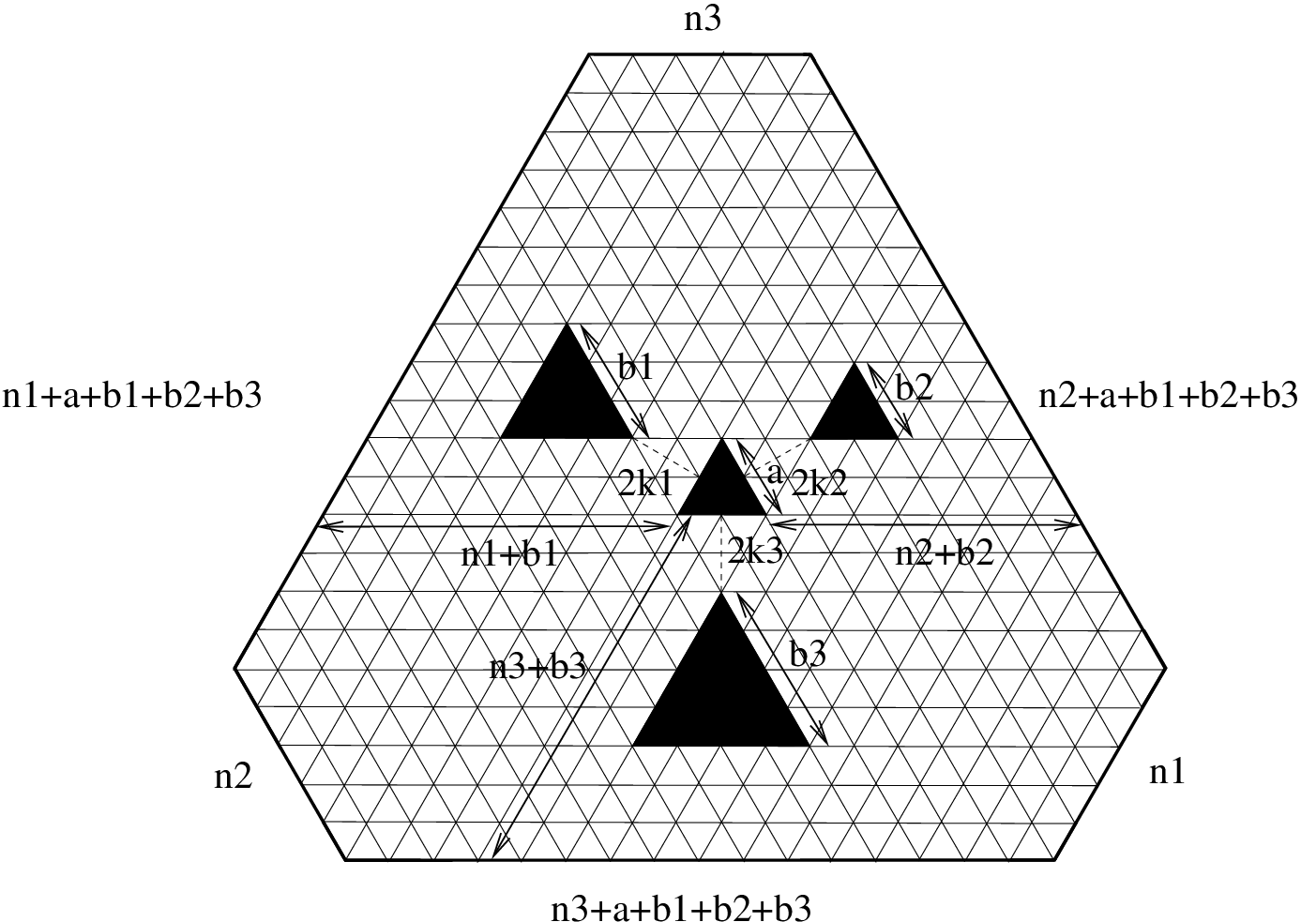
Next we apply this lemma to our setting. However, in order to be able to extend the determinantal formula for even bb to odd bb, we need to work with satellites of independent sizes. It is not more difficult to consider a multivariate generalization, where also the three sides — originally of length nn — are allowed to have independent lengths, and so are the distances between the core and the satellites.

For non-negative integers n1,n2,n3,b1,b2,b3,k1,k2,k3n_{1},n_{2},n_{3},b_{1},b_{2},b_{3},k_{1},k_{2},k_{3} and non-negative even aa, we denote the hexagon with side lengths n1+a+b1+b2+b3,n3,n2+a+b1+b2+b3,n1,n3+a+b1+b2+b3,n2n_{1}+a+b_{1}+b_{2}+b_{3},n_{3},n_{2}+a+b_{1}+b_{2}+b_{3},n_{1},n_{3}+a+b_{1}+b_{2}+b_{3},n_{2} (clockwise from the northwestern side) that has four triangular holes with side lengths a,b1,b2,b3a,b_{1},b_{2},b_{3}, respectively, as indicated in Figure 6 by Sn1,n2,n3,a,b1,b2,b3,k1,k2,k3S_{n_{1},n_{2},n_{3},a,b_{1},b_{2},b_{3},k_{1},k_{2},k_{3}}: The hole of size aa (the core) has distance (n1+b1)⋅32(n_{1}+b_{1})\cdot\frac{\sqrt{3}}{2}, (n2+b2)⋅32(n_{2}+b_{2})\cdot\frac{\sqrt{3}}{2}, (n3+b3)⋅32(n_{3}+b_{3})\cdot\frac{\sqrt{3}}{2} from the three sides of length n1+a+b1+b2+b3n_{1}+a+b_{1}+b_{2}+b_{3}, n2+a+b1+b2+b3n_{2}+a+b_{1}+b_{2}+b_{3}, n3+a+b1+b2+b3n_{3}+a+b_{1}+b_{2}+b_{3}, respectively. The three holes of size b1,b2,b3b_{1},b_{2},b_{3} (the satellites) point towards the center of the core and have distance 2​k1⋅32,2​k2⋅32,2​k3⋅322k_{1}\cdot\frac{\sqrt{3}}{2},2k_{2}\cdot\frac{\sqrt{3}}{2},2k_{3}\cdot\frac{\sqrt{3}}{2} from the core, respectively, where the satellite of size bib_{i} is situated between the core and the long side of the hexagon that has distance ni+bin_{i}+b_{i} from the core.

Note that the geometry of the configuration implies

n1≤a+n2+b2+n3+b3.n_{1}\leq a+n_{2}+b_{2}+n_{3}+b_{3}. (4.2)

This can be seen as follows: Consider the line that includes the “//”-side of the core. The length of the portion of this line included in the wedge obtained by extending the sides of length n2+a+b1+b2+b3n_{2}+a+b_{1}+b_{2}+b_{3} and n3+a+b1+b2+b3n_{3}+a+b_{1}+b_{2}+b_{3} until they meet, which is a+n2+b2+n3+b3a+n_{2}+b_{2}+n_{3}+b_{3}, needs to be at least as large as the length of the southeastern edge of the hexagon, which is n1n_{1}. By symmetry, we also have n2≤a+n1+b1+n3+b3n_{2}\leq a+n_{1}+b_{1}+n_{3}+b_{3} and n3≤a+n1+b1+n2+b2n_{3}\leq a+n_{1}+b_{1}+n_{2}+b_{2}.

Refer to caption
Figure 6. Independent satellites
Refer to caption
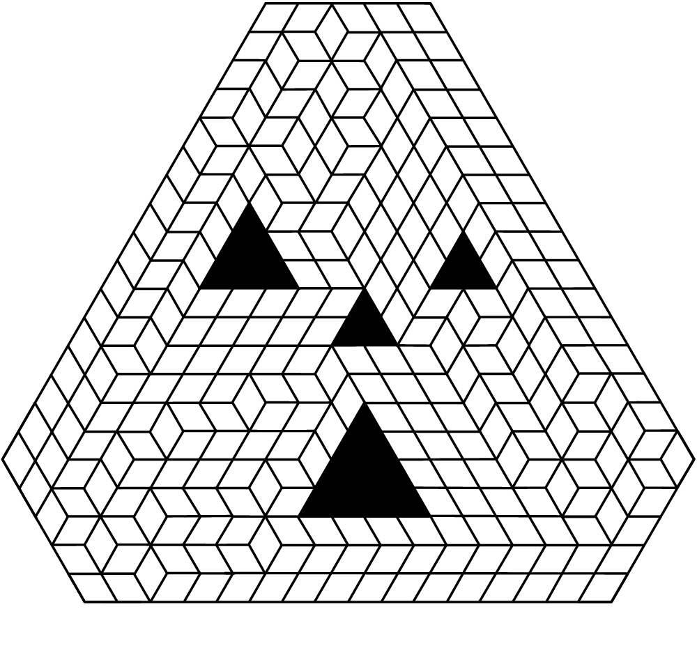
Figure 7. An example of a lozenge tiling of S5,5,5,2,3,2,4,1,1,1S_{5,5,5,2,3,2,4,1,1,1}

If b1,b2,b3b_{1},b_{2},b_{3} are even, Lemma 1 can be applied to compute the number of lozenge tilings of this region. Indeed, set n=n1+n2+a+b1+b2+b3n=n_{1}+n_{2}+a+b_{1}+b_{2}+b_{3}. In order to start from an (n,n+n3)(n,n+n_{3})-trapezoid, we add a triangle of size n2n_{2} at the bottom left corner of the hexagon, while we add a triangle of size n1n_{1} at the bottom right corner. We have six chains of triangles to be removed as follows.

  1. (1)

    At height 001010 10 The height of a removed triangle is one less than its row number. of length n2n_{2} in positions 1,…,n21,\ldots,n_{2}.

  2. (2)

    At height 00 of length n1n_{1} in positions n2+n3+a+b1+b2+b3+1,…,n1+n2+n3+a+b1+b2+b3n_{2}+n_{3}+a+b_{1}+b_{2}+b_{3}+1,\ldots,n_{1}+n_{2}+n_{3}+a+b_{1}+b_{2}+b_{3}.

  3. (3)

    At height n3−2​k3n_{3}-2k_{3} of length b3b_{3} in positions n1+a2+b1+k3+1,…,n1+a2+b1+b3+k3n_{1}+\frac{a}{2}+b_{1}+k_{3}+1,\ldots,n_{1}+\frac{a}{2}+b_{1}+b_{3}+k_{3}.

  4. (4)

    At height n3+b3n_{3}+b_{3} of length aa in positions n1+b1+1,…,n1+a+b1n_{1}+b_{1}+1,\ldots,n_{1}+a+b_{1}.

  5. (5)

    At height n3+a2+b3+k1n_{3}+\frac{a}{2}+b_{3}+k_{1} of length b1b_{1} in positions n1−2​k1+1,…,n1−2​k1+b1n_{1}-2k_{1}+1,\ldots,n_{1}-2k_{1}+b_{1}.

  6. (6)

    At height n3+a2+b3+k2n_{3}+\frac{a}{2}+b_{3}+k_{2} of length b2b_{2} in positions n1+a2+b1+k2+1,…,n1+a2+b1+b2+k2n_{1}+\frac{a}{2}+b_{1}+k_{2}+1,\ldots,n_{1}+\frac{a}{2}+b_{1}+b_{2}+k_{2}.

Using Lemma 1, it follows that the number of lozenge tilings of Sn1,n2,n3,a,b1,b2,b3,k1,k2,k3S_{n_{1},n_{2},n_{3},a,b_{1},b_{2},b_{3},k_{1},k_{2},k_{3}} is

|∏i=1b3Δc3,in3−2​k3​∏i=1aΔc4,in3+b3​∏i=1b1Δc5,in3+a2+b3+k1​∏i=1b2Δc6,in3+a2+b3+k2​det((c1,i−dj−1)1≤i≤n2(c2,i−dj−1)1≤i≤n1(c3,i−dj−1)1≤i≤b3(c4,i−dj−1)1≤i≤a(c5,i−dj−1)1≤i≤b1(c6,i−dj−1)1≤i≤b2)1≤j≤n|,\left|\prod_{i=1}^{b_{3}}\Delta_{c_{3,i}}^{n_{3}-2k_{3}}\prod_{i=1}^{a}\Delta_{c_{4,i}}^{n_{3}+b_{3}}\prod_{i=1}^{b_{1}}\Delta_{c_{5,i}}^{n_{3}+\frac{a}{2}+b_{3}+k_{1}}\prod_{i=1}^{b_{2}}\Delta_{c_{6,i}}^{n_{3}+\frac{a}{2}+b_{3}+k_{2}}\det\left(\begin{array}[]{cc}\binom{c_{1,i}-d}{j-1}&\quad{1\leq i\leq n_{2}}\\ \binom{c_{2,i}-d}{j-1}&\quad{1\leq i\leq n_{1}}\\ \binom{c_{3,i}-d}{j-1}&\quad{1\leq i\leq b_{3}}\\ \binom{c_{4,i}-d}{j-1}&\quad{1\leq i\leq a}\\ \binom{c_{5,i}-d}{j-1}&\quad{1\leq i\leq b_{1}}\\ \binom{c_{6,i}-d}{j-1}&\quad{1\leq i\leq b_{2}}\end{array}\right)_{1\leq j\leq n}\right|, (4.3)

where c1,i=ic_{1,i}=i, c2,i=n2+n3+a+b1+b2+b3+ic_{2,i}=n_{2}+n_{3}+a+b_{1}+b_{2}+b_{3}+i, c3,i=n1+a2+b1+k3+ic_{3,i}=n_{1}+\frac{a}{2}+b_{1}+k_{3}+i, c4,i=n1+b1+ic_{4,i}=n_{1}+b_{1}+i, c5,i=n1−2​k1+ic_{5,i}=n_{1}-2k_{1}+i and c6,i=n1+a2+b1+k2+ic_{6,i}=n_{1}+\frac{a}{2}+b_{1}+k_{2}+i. We obtain the following result.

Proposition 1.

For even b1,b2,b3b_{1},b_{2},b_{3}, we have

M⁡(Sn1,n2,n3,a,b1,b2,b3,k1,k2,k3)=|det((i−dj−1)1≤i≤n2(n2+n3+a+b1+b2+b3+i−dj−1)1≤i≤n1(n1+a2+b1+k3+i−dj−1−n3+2​k3)1≤i≤b3(n1+b1+i−dj−1−n3−b3)1≤i≤a(n1−2​k1+i−dj−1−n3−a2−b3−k1)1≤i≤b1(n1+a2+b1+k2+i−dj−1−n3−a2−b3−k2)1≤i≤b2)1≤j≤n|,\operatorname{M}(S_{n_{1},n_{2},n_{3},a,b_{1},b_{2},b_{3},k_{1},k_{2},k_{3}})=\left|\det\left(\begin{matrix}[l]\binom{i-d}{j-1}&{1\leq i\leq n_{2}}\vskip 5.69054pt\\ \binom{n_{2}+n_{3}+a+b_{1}+b_{2}+b_{3}+i-d}{j-1}&{1\leq i\leq n_{1}}\vskip 5.69054pt\\ \binom{n_{1}+\frac{a}{2}+b_{1}+k_{3}+i-d}{j-1-n_{3}+2k_{3}}&{1\leq i\leq b_{3}}\vskip 5.69054pt\\ \binom{n_{1}+b_{1}+i-d}{j-1-n_{3}-b_{3}}&{1\leq i\leq a}\vskip 5.69054pt\\ \binom{n_{1}-2k_{1}+i-d}{j-1-n_{3}-\frac{a}{2}-b_{3}-k_{1}}&{1\leq i\leq b_{1}}\vskip 5.69054pt\\ \binom{n_{1}+\frac{a}{2}+b_{1}+k_{2}+i-d}{j-1-n_{3}-\frac{a}{2}-b_{3}-k_{2}}&{1\leq i\leq b_{2}}\end{matrix}\right)_{1\leq j\leq n}\right|, (4.4)

where dd can be chosen arbitrarily.

4.2. Polynomiality in the sizes of the satellites

The technique we are using to deal with odd-sized satellites is based on the following crucial observation.

Lemma 2.

For any i∈{1,2,3}i\in\{1,2,3\}, the quantity M⁡(Sn1,n2,n3,a,b1,b2,b3,k1,k2,k3)\operatorname{M}(S_{n_{1},n_{2},n_{3},a,b_{1},b_{2},b_{3},k_{1},k_{2},k_{3}}) is a polynomial in bib_{i} when fixing the nin_{i}’s, the kik_{i}’s, the core size aa, and the two bjb_{j}’s with j≠ij\not=i.

Proof.

We follow the ideas provided in [9, Section 6], which were used there to show the polynomiality of M⁡(Sn,n,n,a,0,0,0,0,0,0)\operatorname{M}(S_{n,n,n,a,0,0,0,0,0,0}) in aa. By symmetry, it suffices to consider the case i=2i=2.

Set S=Sn1,n2,n3,a,b1,b2,b3,k1,k2,k3S=S_{n_{1},n_{2},n_{3},a,b_{1},b_{2},b_{3},k_{1},k_{2},k_{3}}. Let RR be the smallest lattice hexagon that contains the southwestern side of SS, the core, and the satellites of side-lengths b1b_{1} and b3b_{3}. For the region in Figure 7, the resulting region RR is shown on the lower left in Figure 8 (delimited by the dashed line).

Refer to caption

Figure 8. Proving polynomiality in b2b_{2}: The region RR on the lower left delimited by the dashed line does not change as b2b_{2} varies; the lozenges that straddle the dashed line in one of its fixed number (independent of b2b_{2}) of tilings are indicated. The number of ways each such tiling of RR can be extended to a tiling of Sn1,n2,n3,a,b1,b2,b3,k1,k2,k3S_{n_{1},n_{2},n_{3},a,b_{1},b_{2},b_{3},k_{1},k_{2},k_{3}} is polynomial in b2b_{2} for fixed n1,n2,n3,a,b1,b3,k1,k2,k3n_{1},n_{2},n_{3},a,b_{1},b_{3},k_{1},k_{2},k_{3}, by the argument in [9].

As b2b_{2} varies over the non-negative integers (with all the other parameters having fixed values), the region RR does not change. In particular, the number of lozenge tilings of RR in which the dashed portion of the boundary is treated as free (i.e. lozenges are allowed to protrude halfway across them) is a fixed number, independent of b2b_{2}.

One instance of such a tiling (for focus, only the lozenges straddling the dashed line) is shown in Figure 8. By the observation in the previous paragraph, it suffices to show that for any such fixed choice of lozenges straddling the dashed line, the complement R′R^{\prime} of RR in SS — which does change as b2b_{2} varies — has a number of tilings that is a polynomial in b2b_{2}.

This follows by the very same arguments we used in Section 6 of [9]. Indeed, extend rays from the satellite of side b2b_{2} as indicated by the thick solid lines in Figure 8. Depending on the actual values of the fixed parameters n1,n2,n3,a,b1,b3,k1,k2,k3n_{1},n_{2},n_{3},a,b_{1},b_{3},k_{1},k_{2},k_{3}, the ray going southwest may intersect either the NE or SE side of RR. Similarly, the ray going east intersects either the NE or the SE side of SS, and the ray going northwest either the N or the NW side of SS. Figure 8 shows one of these possibilities. We prove polynomiality of M⁡(R′)\operatorname{M}(R^{\prime}) in b2b_{2} in this case; the others follow the same way.

As we did in [9], we partition the lozenge tilings of R′R^{\prime} that have a fixed set ℒ\mathcal{L} of lozenges straddling the dashed line according to the sets of lozenges ℒ1\mathcal{L}_{1}, ℒ2\mathcal{L}_{2} and ℒ3\mathcal{L}_{3} that straddle each of the three rays. Of key importance is the fact that the length each of these rays runs in R′R^{\prime} has a fixed value, independent of b2b_{2}. It therefore suffices to show that for each fixed choice of the position of the lozenges in ℒ\mathcal{L}, ℒ1\mathcal{L}_{1}, ℒ2\mathcal{L}_{2} and ℒ3\mathcal{L}_{3}, the number of lozenge tilings of R′R^{\prime} that contain these lozenges is a polynomial in b2b_{2}.

Clearly, this number is the product of the number of corresponding tilings of the three regions that the rays divide R′R^{\prime} into. For each of these three regions, encode their tilings as families of paths of lozenges (equivalently, lattice paths on ℤ2\mathbb{Z}^{2}) as indicated in Figure 8. Then by the Lindström-Gessel-Viennot theorem [40, 29], the number of tilings of each of these three regions is equal to a determinant whose order is independent of b2b_{2}, and all of whose entries are — as can be easily checked — either independent of b2b_{2}, or of the form (b2+cd)b_{2}+c\choose d, with cc and dd independent of b2b_{2}. This implies that each of them is a polynomial in b2b_{2}, and the proof is complete. ∎

4.3. A determinantal formula for general b1,b2,b3b_{1},b_{2},b_{3} assuming k2=k3k_{2}=k_{3}

The goal of this section is to derive the following determinantal formula for M⁡(Sn1,n2,n3,a,b1,b2,b3,k1,k2,k2)\operatorname{M}(S_{n_{1},n_{2},n_{3},a,b_{1},b_{2},b_{3},k_{1},k_{2},k_{2}}) that holds for general b1,b2,b3b_{1},b_{2},b_{3}. Note that we assume k2=k3k_{2}=k_{3} because the situation is simpler then, but the procedure can be adapted so that it works also if k2≠k3k_{2}\not=k_{3}. In this formula, we use the convention

∑i=abp(i)=−∑i=b+1a−1p(i)\sum_{i=a}^{b}p(i)=-\sum_{i=b+1}^{a-1}p(i)

if b<ab<a. Note that this implies ∑i=aa−1p⁡(i)=0\sum\limits_{i=a}^{a-1}p(i)=0.

Theorem 5.

For all non-negative integers n1,n2,n3,b1,b2,b3,k1,k2n_{1},n_{2},n_{3},b_{1},b_{2},b_{3},k_{1},k_{2} and even aa, we have

M⁡(Sn1,n2,n3,a,b1,b2,b3,k1,k2,k2)=|det((−1)[j≥n3−2k2+1]b3((i−n1−a2−b1−k2−1j−1)+((−1)b1−1)∑q=n3+a2+b3+k1+1j(i−n1+2​k1−1q−1)(−2​k1−a2−b1−k2j−q))1≤i≤n2(−1)[j≥n3+a2+b3+k2+1]b2(−n1+n2+n3+a2+b2+b3−k2+i−1j−1)1≤i≤n1(i−1j−1−n3+2​k2)1≤i≤b3(OPENi−a2−k2−1)j−1−n3−b3)1≤i≤a(−a2−b1−2​k1−k2+i−1j−1−n3−a2−b3−k1)1≤i≤b1(i−1j−1−n3−a2−b3−k2)1≤i≤b2)1≤j≤n|,\operatorname{M}(S_{n_{1},n_{2},n_{3},a,b_{1},b_{2},b_{3},k_{1},k_{2},k_{2}})\\ =\left|\det\left(\begin{array}[]{ll}(-1)^{[j\geq n_{3}-2k_{2}+1]b_{3}}\left(\binom{i-n_{1}-\frac{a}{2}-b_{1}-k_{2}-1}{j-1}\right.\\ \left.\quad+((-1)^{b_{1}}-1)\sum\limits_{q=n_{3}+\frac{a}{2}+b_{3}+k_{1}+1}^{j}\binom{i-n_{1}+2k_{1}-1}{q-1}\binom{-2k_{1}-\frac{a}{2}-b_{1}-k_{2}}{j-q}\right)&{1\leq i\leq n_{2}}\\ \hline\cr(-1)^{[j\geq n_{3}+\frac{a}{2}+b_{3}+k_{2}+1]b_{2}}\binom{-n_{1}+n_{2}+n_{3}+\frac{a}{2}+b_{2}+b_{3}-k_{2}+i-1}{j-1}&{1\leq i\leq n_{1}}\\ \hline\cr\binom{i-1}{j-1-n_{3}+2k_{2}}&{1\leq i\leq b_{3}}\\ \hline\cr\binom{i-\frac{a}{2}-k_{2}-1)}{j-1-n_{3}-b_{3}}&{1\leq i\leq a}\\ \hline\cr\binom{-\frac{a}{2}-b_{1}-2k_{1}-k_{2}+i-1}{j-1-n_{3}-\frac{a}{2}-b_{3}-k_{1}}&{1\leq i\leq b_{1}}\\ \hline\cr\binom{i-1}{j-1-n_{3}-\frac{a}{2}-b_{3}-k_{2}}&{1\leq i\leq b_{2}}\end{array}\right)_{1\leq j\leq n}\right|,

where we use the Iverson bracket which is defined as

[statement]={1if the statement is true0otherwise.[\text{statement}]=\begin{cases}1&\text{if the statement is true}\\ 0&\text{otherwise}\end{cases}.
Proof.

We set d=d1=n1−2​k1+1d=d_{1}=n_{1}-2k_{1}+1 in the determinant in (4.4). Then all entries in the first row of the fifth block (which is the one corresponding to the satellite of size b1b_{1}) are zero except for the one in column j=1+n3+a2+b3+k1j=1+n_{3}+\frac{a}{2}+b_{3}+k_{1}. We expand with respect to this row. The new top row of the fifth block has again only a non-zero entry in column j=1+n3+a2+b3+k1j=1+n_{3}+\frac{a}{2}+b_{3}+k_{1}, and so we expand with respect to this row now. We keep doing this until the fifth block has vanished and obtain

(−1)(n1+n2+n3+3​a2+k1)​b1​det((i−d1j−1)1≤i≤n2(n2+n3+a+b1+b2+b3+i−d1j−1)1≤i≤n1(n1+a2+b1+k3+i−d1j−1−n3+2​k2)1≤i≤b3(n1+b1+i−d1j−1−n3−b3)1≤i≤a(n1+a2+b1+k2+i−d1j−1−n3−a2−b3−k2)1≤i≤b2)1≤j≤n3+a2+b3+k1n3+a2+b1+b3+k1+1≤j≤n.(-1)^{(n_{1}+n_{2}+n_{3}+\frac{3a}{2}+k_{1})b_{1}}\det\left(\begin{matrix}[l]\binom{i-d_{1}}{j-1}&{1\leq i\leq n_{2}}\vskip 5.69054pt\\ \binom{n_{2}+n_{3}+a+b_{1}+b_{2}+b_{3}+i-d_{1}}{j-1}&{1\leq i\leq n_{1}}\vskip 5.69054pt\\ \binom{n_{1}+\frac{a}{2}+b_{1}+k_{3}+i-d_{1}}{j-1-n_{3}+2k_{2}}&{1\leq i\leq b_{3}}\vskip 5.69054pt\\ \binom{n_{1}+b_{1}+i-d_{1}}{j-1-n_{3}-b_{3}}&{1\leq i\leq a}\vskip 5.69054pt\\ \binom{n_{1}+\frac{a}{2}+b_{1}+k_{2}+i-d_{1}}{j-1-n_{3}-\frac{a}{2}-b_{3}-k_{2}}&{1\leq i\leq b_{2}}\end{matrix}\right)_{1\leq j\leq n_{3}+\frac{a}{2}+b_{3}+k_{1}\atop n_{3}+\frac{a}{2}+b_{1}+b_{3}+k_{1}+1\leq j\leq n}.

This can also be written as follows (omitting now the ranges for the rows ii).

(−1)(n1+n2+n3+3​a2+k1)​b1×det((i−d1j−1)1≤j≤n3+a2+b3+k1(i−d1j+n3+a2+b1+b3+k1−1)1≤j≤n1+n2−n3+a2+b2−k1(n2+n3+a+b1+b2+b3+i−d1j−1)1≤j≤n3+a2+b3+k1(n2+n3+a+b1+b2+b3+i−d1j+n3+a2+b1+b3+k1−1)1≤j≤n1+n2−n3+a2+b2−k1(n1+a2+b1+k3+i−d1j−1−n3+2​k2)1≤j≤n3+a2+b3+k1(n1+a2+b1+k3+i−d1j+n3+a2+b1+b3+k1−1−n3+2​k2)1≤j≤n1+n2−n3+a2+b2−k1(n1+b1+i−d1j−1−n3−b3)1≤j≤n3+a2+b3+k1(n1+b1+i−d1j+n3+a2+b1+b3+k1−1−n3−b3)1≤j≤n1+n2−n3+a2+b2−k1(n1+a2+b1+k2+i−d1j−1−n3−a2−b3−k2)1≤j≤n3+a2+b3+k1(n1+a2+b1+k2+i−d1j+n3+a2+b1+b3+k1−1−n3−a2−b3−k2)1≤j≤n1+n2−n3+a2+b2−k1)(-1)^{(n_{1}+n_{2}+n_{3}+\frac{3a}{2}+k_{1})b_{1}}\\ \times\det\left(\begin{array}[]{l|l}\binom{i-d_{1}}{j-1}_{1\leq j\leq n_{3}+\frac{a}{2}+b_{3}+k_{1}}&\binom{i-d_{1}}{j+n_{3}+\frac{a}{2}+b_{1}+b_{3}+k_{1}-1}_{1\leq j\leq n_{1}+n_{2}-n_{3}+\frac{a}{2}+b_{2}-k_{1}}\\ \hline\cr\binom{n_{2}+n_{3}+a+b_{1}+b_{2}+b_{3}+i-d_{1}}{j-1}_{1\leq j\leq n_{3}+\frac{a}{2}+b_{3}+k_{1}}&\binom{n_{2}+n_{3}+a+b_{1}+b_{2}+b_{3}+i-d_{1}}{j+n_{3}+\frac{a}{2}+b_{1}+b_{3}+k_{1}-1}_{1\leq j\leq n_{1}+n_{2}-n_{3}+\frac{a}{2}+b_{2}-k_{1}}\\ \hline\cr\binom{n_{1}+\frac{a}{2}+b_{1}+k_{3}+i-d_{1}}{j-1-n_{3}+2k_{2}}_{1\leq j\leq n_{3}+\frac{a}{2}+b_{3}+k_{1}}&\binom{n_{1}+\frac{a}{2}+b_{1}+k_{3}+i-d_{1}}{j+n_{3}+\frac{a}{2}+b_{1}+b_{3}+k_{1}-1-n_{3}+2k_{2}}_{1\leq j\leq n_{1}+n_{2}-n_{3}+\frac{a}{2}+b_{2}-k_{1}}\\ \hline\cr\binom{n_{1}+b_{1}+i-d_{1}}{j-1-n_{3}-b_{3}}_{1\leq j\leq n_{3}+\frac{a}{2}+b_{3}+k_{1}}&\binom{n_{1}+b_{1}+i-d_{1}}{j+n_{3}+\frac{a}{2}+b_{1}+b_{3}+k_{1}-1-n_{3}-b_{3}}_{1\leq j\leq n_{1}+n_{2}-n_{3}+\frac{a}{2}+b_{2}-k_{1}}\\ \hline\cr\binom{n_{1}+\frac{a}{2}+b_{1}+k_{2}+i-d_{1}}{j-1-n_{3}-\frac{a}{2}-b_{3}-k_{2}}_{1\leq j\leq n_{3}+\frac{a}{2}+b_{3}+k_{1}}&\binom{n_{1}+\frac{a}{2}+b_{1}+k_{2}+i-d_{1}}{j+n_{3}+\frac{a}{2}+b_{1}+b_{3}+k_{1}-1-n_{3}-\frac{a}{2}-b_{3}-k_{2}}_{1\leq j\leq n_{1}+n_{2}-n_{3}+\frac{a}{2}+b_{2}-k_{1}}\end{array}\right)

(Concerning the range of the right block, note that n1+n2−n3+a2+b2−k1≥0n_{1}+n_{2}-n_{3}+\frac{a}{2}+b_{2}-k_{1}\geq 0 because of the following: consider the wedge of the line containing the (n1+a+b1+b2+b3)(n_{1}+a+b_{1}+b_{2}+b_{3})-side of the hexagon and of the line containing the (n2+a+b1+b2+b3)(n_{2}+a+b_{1}+b_{2}+b_{3})-side of the hexagon. Then the length of the section of the horizontal line containing the top vertex of the satellite of size b1b_{1} in this wedge is n1+n2+a2+b2−k1n_{1}+n_{2}+\frac{a}{2}+b_{2}-k_{1} which is now obviously greater than or equal to n3n_{3}, the length of the top side of the hexagon.)

Next we will show that we can modify this formula by introducing (−1)b1(-1)^{b_{1}} at various places such that the result is a polynomial function in b1b_{1}. Since this has of course no effect if b1b_{1} is even, the modified formula will give the number of lozenge tilings for even b1b_{1}. However, using Lemma 2 and the fact that a polynomial is uniquely determined by its evaluation on even integers, the modified formula gives the number of lozenge tilings for all non-negative integers b1b_{1} (however still assuming that b2b_{2} and b3b_{3} are even).

The following observations are crucial:

  • •

    The entries in the first n3+a2+b3+k1n_{3}+\frac{a}{2}+b_{3}+k_{1} columns are all polynomials in b1b_{1}, since b1b_{1} appears at most in the upper parameter of the binomial coefficient.

  • •

    The entries that are right of column n3+a2+b3+k1n_{3}+\frac{a}{2}+b_{3}+k_{1} and below row n2n_{2} are also polynomials in b1b_{1}: These entries are binomial coefficients of the form (b1+sb1+t)\binom{b_{1}+s}{b_{1}+t} for some integers ss and tt. We have b1+s≥0b_{1}+s\geq 0 which follows basically because the satellite of size b1b_{1} is the leftmost removed (big) triangle except for the triangle of size n2n_{2}, which however corresponds to the top block (see also (4.2)). Thus we can apply the symmetry of the binomial coefficient, i.e.,

    (nk)=(nn−k)if n≥0,\binom{n}{k}=\binom{n}{n-k}\quad\text{if $n\geq 0$}, (4.5)

    to obtain binomial coefficients where b1b_{1} only appears in the top parameter.

  • •

    As for the remaining entries in row 11 to n2n_{2}, they are binomial coefficients of the form (sb1+t)\binom{s}{b_{1}+t} where s<b1+ts<b_{1}+t. In order to see this, observe that the extreme case with regard to this inequality is when i=n2i=n_{2} and j=1j=1. In this case we need to show that

    n2≤(n3+a2+b3+k1)+b1+(n1−2​k1).n_{2}\leq\left(n_{3}+\frac{a}{2}+b_{3}+k_{1}\right)+b_{1}+\left(n_{1}-2k_{1}\right).

    However, this is obvious: n3+a2+b3+k1n_{3}+\frac{a}{2}+b_{3}+k_{1} is the “lattice” distance of the satellite of size b1b_{1} from the bottom of the hexagon, thus (n3+a2+b3+k1)+b1\left(n_{3}+\frac{a}{2}+b_{3}+k_{1}\right)+b_{1} is the “lattice” distance between the top of this satellite to the bottom of the hexagon and going n1−2​k1n_{1}-2k_{1} unit steps from this top into ↖\nwarrow-direction will bring us to a point on the side of length n1+a+b1+b2+b3n_{1}+a+b_{1}+b_{2}+b_{3}, which is thus surely above the side of length n2n_{2}.

    We claim that this implies that (−1)b1​(sb1+t)(-1)^{b_{1}}\binom{s}{b_{1}+t} is polynomial in b1b_{1}: We use the second elementary transformation for binomial coefficients, i.e.,

    (nk)=(−1)k​(k−n−1k)\binom{n}{k}=(-1)^{k}\binom{k-n-1}{k} (4.6)

    to see that

    (sb1+t)=(−1)b1+t​(b1+t−s−1b1+t)=(−1)b1+t​(b1+t−s−1−s−1),\binom{s}{b_{1}+t}=(-1)^{b_{1}+t}\binom{b_{1}+t-s-1}{b_{1}+t}=(-1)^{b_{1}+t}\binom{b_{1}+t-s-1}{-s-1},

    where the last step follows from the symmetry (4.5) which can be applied since b1+t−s−1≥0b_{1}+t-s-1\geq 0.

It follows that we obtain a formula that is a polynomial function in b1b_{1} and coincides with the original formula for even b1b_{1} if we do the following:

  • •

    Multiply the expression with (−1)(n1+n2+n3+3​a2+k1)​b1(-1)^{(n_{1}+n_{2}+n_{3}+\frac{3a}{2}+k_{1})b_{1}}.

  • •

    Multiply the entries in the first n2n_{2} rows and right of column n3+a2+b3+k1n_{3}+\frac{a}{2}+b_{3}+k_{1} with (−1)b1(-1)^{b_{1}}.

If we “reverse” after this modification our calculation so that we again have a block that corresponds to the satellite of size b1b_{1}, we obtain

(−1)(n1+n2+n3+3​a2+k1)​b1​∏i=1b3Δc3,in3−2​k3​∏i=1aΔc4,in3+b3​∏i=1b1Δc5,in3+a2+b3+k1​∏i=1b2Δc6,in3+a2+b3+k2det((c1,i−d1j−1)(−1)[j≥n3+a2+b1+b3+k1+1]b11≤i≤n2(c2,i−d1j−1)1≤i≤n1(c3,i−d1j−1)1≤i≤b3(c4,i−d1j−1)1≤i≤a(c5,i−d1j−1)1≤i≤b1(c6,i−d1j−1)1≤i≤b2)1≤j≤n(-1)^{(n_{1}+n_{2}+n_{3}+\frac{3a}{2}+k_{1})b_{1}}\prod_{i=1}^{b_{3}}\Delta_{c_{3,i}}^{n_{3}-2k_{3}}\prod_{i=1}^{a}\Delta_{c_{4,i}}^{n_{3}+b_{3}}\prod_{i=1}^{b_{1}}\Delta_{c_{5,i}}^{n_{3}+\frac{a}{2}+b_{3}+k_{1}}\prod_{i=1}^{b_{2}}\Delta_{c_{6,i}}^{n_{3}+\frac{a}{2}+b_{3}+k_{2}}\\ \det\left(\begin{matrix}[l]\binom{c_{1,i}-d_{1}}{j-1}(-1)^{[j\geq n_{3}+\frac{a}{2}+b_{1}+b_{3}+k_{1}+1]b_{1}}&{1\leq i\leq n_{2}}\vskip 5.69054pt\\ \binom{c_{2,i}-d_{1}}{j-1}&{1\leq i\leq n_{1}}\vskip 5.69054pt\\ \binom{c_{3,i}-d_{1}}{j-1}&{1\leq i\leq b_{3}}\vskip 5.69054pt\\ \binom{c_{4,i}-d_{1}}{j-1}&{1\leq i\leq a}\vskip 5.69054pt\\ \binom{c_{5,i}-d_{1}}{j-1}&{1\leq i\leq b_{1}}\vskip 5.69054pt\\ \binom{c_{6,i}-d_{1}}{j-1}&{1\leq i\leq b_{2}}\end{matrix}\right)_{1\leq j\leq n}

at c1,i=i,c_{1,i}=i, c2,i=n2+n3+a+b1+b2+b3+ic_{2,i}=n_{2}+n_{3}+a+b_{1}+b_{2}+b_{3}+i,c3,i=n1+a2+b1+k2+ic_{3,i}=n_{1}+\frac{a}{2}+b_{1}+k_{2}+i, c4,i=n1+b1+ic_{4,i}=n_{1}+b_{1}+i, c5,i=n1−2​k1+ic_{5,i}=n_{1}-2k_{1}+i, c6,i=n1+a2+b1+k2+ic_{6,i}=n_{1}+\frac{a}{2}+b_{1}+k_{2}+i, provided that d1=n1−2​k1+1d_{1}=n_{1}-2k_{1}+1. Note that (−1)[j≥n3+a2+b1+b3+k1+1]b1(-1)^{[j\geq n_{3}+\frac{a}{2}+b_{1}+b_{3}+k_{1}+1]b_{1}} can actually be replaced by any (−1)[j≥n3+a2+l+b3+k1+1]b1(-1)^{[j\geq n_{3}+\frac{a}{2}+l+b_{3}+k_{1}+1]b_{1}} with 0≤l≤b10\leq l\leq b_{1}: when “eliminating” a block it becomes apparent that the values of certain entries do not play a role at all. When we reverse the procedure, we are free to choose the values conveniently. We choose l=0l=0 in the following.

Now observe that, by the Chu-Vandermonde summation,

(c−d2j−1)=∑q=1j(c−d1q−1)​(d1−d2j−q),\binom{c-d_{2}}{j-1}=\sum_{q=1}^{j}\binom{c-d_{1}}{q-1}\binom{d_{1}-d_{2}}{j-q},

and multiply the matrix underlying the determinant from the right with the upper triangular matrix ((d1−d2j−i))1≤i,j≤n(\binom{d_{1}-d_{2}}{j-i})_{1\leq i,j\leq n} with determinant 11. This gives the following matrix.

((c1,i−d2j−1)+((−1)b1−1)​∑q=n3+a2+b3+k1+1j(c1,i−d1q−1)​(d1−d2j−q)1≤i≤n2(c2,i−d2j−1)1≤i≤n1(c3,i−d2j−1)1≤i≤b3(c4,i−d2j−1)1≤i≤a(c5,i−d2j−1)1≤i≤b1(c6,i−d2j−1)1≤i≤b2)1≤j≤n\left(\begin{matrix}[l]\binom{c_{1,i}-d_{2}}{j-1}+((-1)^{b_{1}}-1)\sum\limits_{q=n_{3}+\frac{a}{2}+b_{3}+k_{1}+1}^{j}\binom{c_{1,i}-d_{1}}{q-1}\binom{d_{1}-d_{2}}{j-q}&{1\leq i\leq n_{2}}\vskip 5.69054pt\\ \binom{c_{2,i}-d_{2}}{j-1}&{1\leq i\leq n_{1}}\vskip 5.69054pt\\ \binom{c_{3,i}-d_{2}}{j-1}&{1\leq i\leq b_{3}}\vskip 5.69054pt\\ \binom{c_{4,i}-d_{2}}{j-1}&{1\leq i\leq a}\vskip 5.69054pt\\ \binom{c_{5,i}-d_{2}}{j-1}&{1\leq i\leq b_{1}}\vskip 5.69054pt\\ \binom{c_{6,i}-d_{2}}{j-1}&{1\leq i\leq b_{2}}\end{matrix}\right)_{1\leq j\leq n}

Specializing the cl,ic_{l,i}, we obtain the following expression.

(−1)(n1+n2+n3+3​a2+k1)​b1×det((i−d2j−1)+((−1)b1−1)​∑q=n3+a2+b3+k1+1j(i−d1q−1)​(d1−d2j−q)1≤i≤n2(n2+n3+a+b1+b2+b3+i−d2j−1)1≤i≤n1(n1+a2+b1+k2+i−d2j−1−n3+2​k2)1≤i≤b3(n1+b1+i−d2j−1−n3−b3)1≤i≤a(n1−2​k1+i−d2j−1−n3−a2−b3−k1)1≤i≤b1(n1+a2+b1+k2+i−d2j−1−n3−a2−b3−k2)1≤i≤b2)1≤j≤n(-1)^{(n_{1}+n_{2}+n_{3}+\frac{3a}{2}+k_{1})b_{1}}\\ \times\det\left(\begin{matrix}[l]\binom{i-d_{2}}{j-1}+((-1)^{b_{1}}-1)\sum\limits_{q=n_{3}+\frac{a}{2}+b_{3}+k_{1}+1}^{j}\binom{i-d_{1}}{q-1}\binom{d_{1}-d_{2}}{j-q}&{1\leq i\leq n_{2}}\vskip 5.69054pt\\ \binom{n_{2}+n_{3}+a+b_{1}+b_{2}+b_{3}+i-d_{2}}{j-1}&{1\leq i\leq n_{1}}\vskip 5.69054pt\\ \binom{n_{1}+\frac{a}{2}+b_{1}+k_{2}+i-d_{2}}{j-1-n_{3}+2k_{2}}&{1\leq i\leq b_{3}}\vskip 5.69054pt\\ \binom{n_{1}+b_{1}+i-d_{2}}{j-1-n_{3}-b_{3}}&{1\leq i\leq a}\vskip 5.69054pt\\ \binom{n_{1}-2k_{1}+i-d_{2}}{j-1-n_{3}-\frac{a}{2}-b_{3}-k_{1}}&{1\leq i\leq b_{1}}\vskip 5.69054pt\\ \binom{n_{1}+\frac{a}{2}+b_{1}+k_{2}+i-d_{2}}{j-1-n_{3}-\frac{a}{2}-b_{3}-k_{2}}&{1\leq i\leq b_{2}}\end{matrix}\right)_{1\leq j\leq n}

We set d2=n1+a2+b1+k2+1d_{2}=n_{1}+\frac{a}{2}+b_{1}+k_{2}+1. (The assumption k2=k3k_{2}=k_{3} is now useful because it allows us to eliminate the blocks of the satellites of sizes b2b_{2} and b3b_{3} simultaneously.) With this, all entries in first row of the bottom block are zero except for the one in column j=1+n3+a2+b3+k2j=1+n_{3}+\frac{a}{2}+b_{3}+k_{2}, and so we expand with respect to this row. We can keep doing this until the bottom block vanishes and obtain the following.

(−1)(n1+n2+n3+3​a2+k1)​b1+(n1+n2+n3+3​a2+b1+k2)​b2×det((i−d2j−1)+((−1)b1−1)​∑q=n3+a2+b3+k1+1j(i−d1q−1)​(d1−d2j−q)1≤i≤n2(n2+n3+a+b1+b2+b3+i−d2j−1)1≤i≤n1(n1+a2+b1+k2+i−d2j−1−n3+2​k2)1≤i≤b3(n1+b1+i−d2j−1−n3−b3)1≤i≤a(n1−2​k1+i−d2j−1−n3−a2−b3−k1)1≤i≤b1)1≤j≤n3+a2+b3+k2n3+a2+b2+b3+k2+1≤j≤n(-1)^{(n_{1}+n_{2}+n_{3}+\frac{3a}{2}+k_{1})b_{1}+(n_{1}+n_{2}+n_{3}+\frac{3a}{2}+b_{1}+k_{2})b_{2}}\\ \times\det\left(\begin{matrix}[l]\binom{i-d_{2}}{j-1}+((-1)^{b_{1}}-1)\sum\limits_{q=n_{3}+\frac{a}{2}+b_{3}+k_{1}+1}^{j}\binom{i-d_{1}}{q-1}\binom{d_{1}-d_{2}}{j-q}&{1\leq i\leq n_{2}}\vskip 5.69054pt\\ \binom{n_{2}+n_{3}+a+b_{1}+b_{2}+b_{3}+i-d_{2}}{j-1}&{1\leq i\leq n_{1}}\vskip 5.69054pt\\ \binom{n_{1}+\frac{a}{2}+b_{1}+k_{2}+i-d_{2}}{j-1-n_{3}+2k_{2}}&{1\leq i\leq b_{3}}\vskip 5.69054pt\\ \binom{n_{1}+b_{1}+i-d_{2}}{j-1-n_{3}-b_{3}}&{1\leq i\leq a}\vskip 5.69054pt\\ \binom{n_{1}-2k_{1}+i-d_{2}}{j-1-n_{3}-\frac{a}{2}-b_{3}-k_{1}}&{1\leq i\leq b_{1}}\end{matrix}\right)_{1\leq j\leq n_{3}+\frac{a}{2}+b_{3}+k_{2}\atop n_{3}+\frac{a}{2}+b_{2}+b_{3}+k_{2}+1\leq j\leq n}

The first n3+a2+b3+k2n_{3}+\frac{a}{2}+b_{3}+k_{2} columns of the matrix underlying the determinant are

((i−d2j−1)+((−1)b1−1)​∑q=n3+a2+b3+k1+1j(i−d1q−1)​(d1−d2j−q)1≤i≤n2(n2+n3+a+b1+b2+b3+i−d2j−1)1≤i≤n1(n1+a2+b1+k2+i−d2j−1−n3+2​k2)1≤i≤b3(n1+b1+i−d2j−1−n3−b3)1≤i≤a(n1−2​k1+i−d2j−1−n3−a2−b3−k1)1≤i≤b1)1≤j≤n3+a2+b3+k2.\left(\begin{matrix}[l]\binom{i-d_{2}}{j-1}+((-1)^{b_{1}}-1)\sum\limits_{q=n_{3}+\frac{a}{2}+b_{3}+k_{1}+1}^{j}\binom{i-d_{1}}{q-1}\binom{d_{1}-d_{2}}{j-q}&{1\leq i\leq n_{2}}\vskip 5.69054pt\\ \binom{n_{2}+n_{3}+a+b_{1}+b_{2}+b_{3}+i-d_{2}}{j-1}&{1\leq i\leq n_{1}}\vskip 5.69054pt\\ \binom{n_{1}+\frac{a}{2}+b_{1}+k_{2}+i-d_{2}}{j-1-n_{3}+2k_{2}}&{1\leq i\leq b_{3}}\vskip 5.69054pt\\ \binom{n_{1}+b_{1}+i-d_{2}}{j-1-n_{3}-b_{3}}&{1\leq i\leq a}\vskip 5.69054pt\\ \binom{n_{1}-2k_{1}+i-d_{2}}{j-1-n_{3}-\frac{a}{2}-b_{3}-k_{1}}&{1\leq i\leq b_{1}}\end{matrix}\right)_{1\leq j\leq n_{3}+\frac{a}{2}+b_{3}+k_{2}}.

Only the entries in the second block depend on b2b_{2}, and, since b2b_{2} appears only in the upper parameter of the binomial coefficient, these entries are polynomials in b2b_{2}. The matrix consisting of the remaining columns can be written as follows

((i−d2j+n3+a2+b2+b3+k2−1)+((−1)b1−1)​∑q=n3+a2+b3+k1+1j+n3+a2+b2+b3+k2(i−d1q−1)​(d1−d2j+n3+a2+b2+b3+k2−q)1≤i≤n2(n2+n3+a+b1+b2+b3+i−d2j+n3+a2+b2+b3+k2−1)1≤i≤n1(n1+a2+b1+k2+i−d2j+a2+b2+b3+3​k2−1)1≤i≤b3(n1+b1+i−d2j+a2+b2+k2−1)1≤i≤a(n1−2​k1+i−d2j+b2+k2−k1−1)1≤i≤b1),\left(\begin{matrix}[l]\binom{i-d_{2}}{j+n_{3}+\frac{a}{2}+b_{2}+b_{3}+k_{2}-1}+((-1)^{b_{1}}-1)\sum\limits_{q=n_{3}+\frac{a}{2}+b_{3}+k_{1}+1}^{j+n_{3}+\frac{a}{2}+b_{2}+b_{3}+k_{2}}\binom{i-d_{1}}{q-1}\binom{d_{1}-d_{2}}{j+n_{3}+\frac{a}{2}+b_{2}+b_{3}+k_{2}-q}&{1\leq i\leq n_{2}}\vskip 5.69054pt\\ \binom{n_{2}+n_{3}+a+b_{1}+b_{2}+b_{3}+i-d_{2}}{j+n_{3}+\frac{a}{2}+b_{2}+b_{3}+k_{2}-1}&{1\leq i\leq n_{1}}\vskip 5.69054pt\\ \binom{n_{1}+\frac{a}{2}+b_{1}+k_{2}+i-d_{2}}{j+\frac{a}{2}+b_{2}+b_{3}+3k_{2}-1}&{1\leq i\leq b_{3}}\vskip 5.69054pt\\ \binom{n_{1}+b_{1}+i-d_{2}}{j+\frac{a}{2}+b_{2}+k_{2}-1}&{1\leq i\leq a}\vskip 5.69054pt\\ \binom{n_{1}-2k_{1}+i-d_{2}}{j+b_{2}+k_{2}-k_{1}-1}&{1\leq i\leq b_{1}}\end{matrix}\right),

where 1≤j≤n1+n2−n3+a2+b1−k21\leq j\leq n_{1}+n_{2}-n_{3}+\frac{a}{2}+b_{1}-k_{2}. We analyze the different blocks of the matrix:

  • •

    Top block: In (i−d2j+n3+a2+b2+b3+k2−1)\binom{i-d_{2}}{j+n_{3}+\frac{a}{2}+b_{2}+b_{3}+k_{2}-1}, the upper parameter is always less than the lower parameter, and so, in analogy to a situation for b1b_{1}, this binomial coefficient is a polynomial function in b2b_{2} after multiplication with (−1)b2(-1)^{b_{2}}. Now, as d1−d2<0d_{1}-d_{2}<0 (unless b1=0b_{1}=0 in which case the entry simplifies to the binomial coefficient that was already discussed), (d1−d2j+n3+a2+b2+b3+k2−q)\binom{d_{1}-d_{2}}{j+n_{3}+\frac{a}{2}+b_{2}+b_{3}+k_{2}-q} is a polynomial function in b2b_{2} and qq when multiplied with (−1)b2+q(-1)^{b_{2}+q}. In case i−d1i-d_{1} is non-negative, we can sum over all qq less than or equal to i−d1+1i-d_{1}+1 (because otherwise the binomial coefficient (i−d1q−1)\binom{i-d_{1}}{q-1} is zero), and, since b2b_{2} has now disappeared from the upper bound in the summation, the entry is seen to be a polynomial function in b2b_{2} after multiplication with (−1)b2(-1)^{b_{2}}. If, however i−d1i-d_{1} is negative, then (i−d1q−1)\binom{i-d_{1}}{q-1} is a polynomial in qq after multiplication with (−1)q(-1)^{q}, and so the summand (i−d1q−1)​(d1−d2j+n3+a2+b2+b3+k2−q)\binom{i-d_{1}}{q-1}\binom{d_{1}-d_{2}}{j+n_{3}+\frac{a}{2}+b_{2}+b_{3}+k_{2}-q} is a polynomial function in qq. Using the fact that ∑i=abp⁡(i)\sum\limits_{i=a}^{b}p(i) is a polynomial function in aa and bb if p⁡(i)p(i) is a polynomial in ii, it follows that also in this case, the entry is a polynomial function in b2b_{2} after multiplication with (−1)b2(-1)^{b_{2}}.

  • •

    Second block: b2b_{2} appears in the upper parameter as well as in the lower parameter of the binomial coefficient. As the upper parameter is non-negative, the symmetry can be applied in order to remove b2b_{2} from the lower parameter.

  • •

    As for the remaining blocks, the entries are always of the form (sb2+t)\binom{s}{b_{2}+t} where s<b2+ts<b_{2}+t, which implies that these entries are polynomial functions after multiplication with (−1)b2(-1)^{b_{2}}.

Summarizing we see that, in order to transform the determinant formula into a polynomial function in b2b_{2}, we need to do the following.

  • •

    Multiply with (−1)(n1+n2+n3+3​a2+b1+k2)​b2(-1)^{(n_{1}+n_{2}+n_{3}+\frac{3a}{2}+b_{1}+k_{2})b_{2}}.

  • •

    Multiply the entries in the columns right of the column n3+a2+b3+k2n_{3}+\frac{a}{2}+b_{3}+k_{2} with (−1)b2(-1)^{b_{2}}, except for those in the second block.

Since there are n1+n2−n3+a2+b1−k2n_{1}+n_{2}-n_{3}+\frac{a}{2}+b_{1}-k_{2} columns right of the column n3+a2+b3+k2n_{3}+\frac{a}{2}+b_{3}+k_{2}, this is equivalent to the following.

  • •

    Multiply only the entries in the second block right of the column n3+a2+b3+k2n_{3}+\frac{a}{2}+b_{3}+k_{2} with (−1)b2(-1)^{b_{2}}.

Going back in our calculation and reintroducing a block with b2b_{2} rows, we obtain

(−1)(n1+n2+n3+3​a2+k1)​b1×det((i−d2j−1)+((−1)b1−1)​∑q=n3+a2+b3+k1+1j(i−d1q−1)​(d1−d2j−q)1≤i≤n2(−1)[j≥n3+a2+b3+k2+1]b2(n2+n3+a+b1+b3+i−d2j−1)1≤i≤n1(n1+a2+b1+k2+i−d2j−1−n3+2​k2)1≤i≤b3(n1+b1+i−d2j−1−n3−b3)1≤i≤a(n1−2​k1+i−d2j−1−n3−a2−b3−k1)1≤i≤b1(n1+a2+b1+k2+i−d2j−1−n3−a2−b3−k2)1≤i≤b2)1≤j≤n.(-1)^{(n_{1}+n_{2}+n_{3}+\frac{3a}{2}+k_{1})b_{1}}\times\det\left(\begin{matrix}[l]\binom{i-d_{2}}{j-1}+((-1)^{b_{1}}-1)\sum\limits_{q=n_{3}+\frac{a}{2}+b_{3}+k_{1}+1}^{j}\binom{i-d_{1}}{q-1}\binom{d_{1}-d_{2}}{j-q}&{1\leq i\leq n_{2}}\vskip 5.69054pt\\ (-1)^{[j\geq n_{3}+\frac{a}{2}+b_{3}+k_{2}+1]b_{2}}\binom{n_{2}+n_{3}+a+b_{1}+b_{3}+i-d_{2}}{j-1}&{1\leq i\leq n_{1}}\vskip 5.69054pt\\ \binom{n_{1}+\frac{a}{2}+b_{1}+k_{2}+i-d_{2}}{j-1-n_{3}+2k_{2}}&{1\leq i\leq b_{3}}\vskip 5.69054pt\\ \binom{n_{1}+b_{1}+i-d_{2}}{j-1-n_{3}-b_{3}}&{1\leq i\leq a}\vskip 5.69054pt\\ \binom{n_{1}-2k_{1}+i-d_{2}}{j-1-n_{3}-\frac{a}{2}-b_{3}-k_{1}}&{1\leq i\leq b_{1}}\vskip 5.69054pt\\ \binom{n_{1}+\frac{a}{2}+b_{1}+k_{2}+i-d_{2}}{j-1-n_{3}-\frac{a}{2}-b_{3}-k_{2}}&{1\leq i\leq b_{2}}\end{matrix}\right)_{1\leq j\leq n}.

As for b3b_{3}, a similar argument shows that we need to make the adjustment only in the top block. This concludes the proof of the theorem. ∎

4.4. Polynomiality in aa

The purpose of this section is to modify the formula in Theorem 5 to reveal the polynomiality in aa. More specifically, we prove the following theorem.

Theorem 6.

Let

A=((i−n1−b1−1j−1)+((−1)b3−1)​∑p=1+n3−2​k2j(OPENi−n1−a2−b1−k2−1)p−1)​(a2+k2j−p)1≤i≤n2(−n1+n2+n3+a+b2+b3+i−1j−1)1≤i≤n1(a2+k2+i−1j−1−n3+2​k2)1≤i≤b301≤i≤b101≤i≤b2)1≤j≤n3+b3A=\left(\begin{matrix}[l]\binom{i-n_{1}-b_{1}-1}{j-1} +((-1)^{b_{3}}-1)\sum\limits_{p=1+n_{3}-2k_{2}}^{j}\binom{i-n_{1}-\frac{a}{2}-b_{1}-k_{2}-1)}{p-1}\binom{\frac{a}{2}+k_{2}}{j-p}&1\leq i\leq n_{2}\vskip 5.69054pt\\ \binom{-n_{1}+n_{2}+n_{3}+a+b_{2}+b_{3}+i-1}{j-1}\vskip 5.69054pt&1\leq i\leq n_{1}\\ \binom{\frac{a}{2}+k_{2}+i-1}{j-1-n_{3}+2k_{2}}&1\leq i\leq b_{3}\vskip 5.69054pt\\ 0&1\leq i\leq b_{1}\vskip 5.69054pt\\ 0&1\leq i\leq b_{2}\end{matrix}\right)_{1\leq j\leq n_{3}+b_{3}}

and

B′=((−1)j+n3−1​(n1+n3+a+b1+b3−i+j−1n1+b1−i)+((−1)b1−1)(−1)j+n3−1∑q=n3+a2+b3+k1+1j+n3+a+b3(n1−2​k1−i+q−1n1−2​k1−i)(j+n3+a+b1+b3+2​k1−q−1b1+2​k1−1)1≤i≤n2(−n1+n2+n3+a+b2+b3+i−1−n1+n2+b2+i−j)+((−1)b2−1)∑p=1−n1+n2+b2−2​k2+i(−n1+n2+n3+a2+b2+b3−k2+i−1−n1+n2+b2−2​k2+i−p)(a2+k22​k2−j+p)1≤i≤n101≤i≤b3(−1)j​(a2+b1+k1−i+j−1b1+2​k1−i)1≤i≤b1(a2+k2+i−12​k2+i−j)1≤i≤b2),B^{\prime}=\left(\begin{array}[]{ll}(-1)^{j+n_{3}-1}\binom{n_{1}+n_{3}+a+b_{1}+b_{3}-i+j-1}{n_{1}+b_{1}-i}\\ \quad+\left((-1)^{b_{1}}-1\right)(-1)^{j+n_{3}-1}\sum\limits_{q=n_{3}+\frac{a}{2}+b_{3}+k_{1}+1}^{j+n_{3}+a+b_{3}}\binom{n_{1}-2k_{1}-i+q-1}{n_{1}-2k_{1}-i}\binom{j+n_{3}+a+b_{1}+b_{3}+2k_{1}-q-1}{b_{1}+2k_{1}-1}&1\leq i\leq n_{2}\\ \hline\cr\binom{-n_{1}+n_{2}+n_{3}+a+b_{2}+b_{3}+i-1}{-n_{1}+n_{2}+b_{2}+i-j}\\ \quad+\left((-1)^{b_{2}}-1\right)\sum\limits_{p=1}^{-n_{1}+n_{2}+b_{2}-2k_{2}+i}\binom{-n_{1}+n_{2}+n_{3}+\frac{a}{2}+b_{2}+b_{3}-k_{2}+i-1}{-n_{1}+n_{2}+b_{2}-2k_{2}+i-p}\binom{\frac{a}{2}+k_{2}}{2k_{2}-j+p}&1\leq i\leq n_{1}\\ \hline\cr 0&1\leq i\leq b_{3}\\ \hline\cr(-1)^{j}\binom{\frac{a}{2}+b_{1}+k_{1}-i+j-1}{b_{1}+2k_{1}-i}&1\leq i\leq b_{1}\\ \hline\cr\binom{\frac{a}{2}+k_{2}+i-1}{2k_{2}+i-j}&1\leq i\leq b_{2}\end{array}\right),

where the range of jj in B′B^{\prime} is 1≤j≤n1+n2−n3+b1+b21\leq j\leq n_{1}+n_{2}-n_{3}+b_{1}+b_{2}. Then the number of lozenge tilings of Sn1,n2,n3,a,b1,b2,b3,k1,k2,k2S_{n_{1},n_{2},n_{3},a,b_{1},b_{2},b_{3},k_{1},k_{2},k_{2}} is the absolute value of det(A|B′)\det\left(A\,|\,B^{\prime}\right), which is obviously a polynomial in aa since all matrix entries are polynomials in aa.

Proof.

We need to eliminate the fourth block in the formula in Theorem 5. Note that this formula can also be written (up to sign) as follows:

(−1)(n1+n2+n3+3​a2+k1)​b1+(n1+n2+n3)​b3×∏i=1b3Δc3,in3−2​k2​∏i=1aΔc4,in3+b3​∏i=1b1Δc5,in3+a2+b3+k1​∏i=1b2Δc6,in3+a2+b3+k2det((−1)[j≥1+n3−2k2]b3((c1,i−d2j−1)+((−1)b1−1)∑q=n3+a2+b3+k1+1j(c1,i−d1q−1)(d1−d2j−q))1≤i≤n2(−1)[j≥n3+a2+b3+k2+1]b2(c2,i−d2j−1)1≤i≤n1(c3,i−d2j−1)1≤i≤b3(c4,i−d2j−1)1≤i≤a(c5,i−d2j−1)1≤i≤b1(c6,i−d2j−1)1≤i≤b2)1≤j≤n(-1)^{(n_{1}+n_{2}+n_{3}+\frac{3a}{2}+k_{1})b_{1}+(n_{1}+n_{2}+n_{3})b_{3}}\\ \times\prod_{i=1}^{b_{3}}\Delta_{c_{3,i}}^{n_{3}-2k_{2}}\prod_{i=1}^{a}\Delta_{c_{4,i}}^{n_{3}+b_{3}}\prod_{i=1}^{b_{1}}\Delta_{c_{5,i}}^{n_{3}+\frac{a}{2}+b_{3}+k_{1}}\prod_{i=1}^{b_{2}}\Delta_{c_{6,i}}^{n_{3}+\frac{a}{2}+b_{3}+k_{2}}\\ \det\left(\begin{matrix}[l](-1)^{[j\geq 1+n_{3}-2k_{2}]b_{3}}\left(\binom{c_{1,i}-d_{2}}{j-1}+((-1)^{b_{1}}-1)\sum\limits_{q=n_{3}+\frac{a}{2}+b_{3}+k_{1}+1}^{j}\binom{c_{1,i}-d_{1}}{q-1}\binom{d_{1}-d_{2}}{j-q}\right)&{1\leq i\leq n_{2}}\vskip 5.69054pt\\ (-1)^{[j\geq n_{3}+\frac{a}{2}+b_{3}+k_{2}+1]b_{2}}\binom{c_{2,i}-d_{2}}{j-1}&{1\leq i\leq n_{1}}\vskip 5.69054pt\\ \binom{c_{3,i}-d_{2}}{j-1}&{1\leq i\leq b_{3}}\vskip 5.69054pt\\ \binom{c_{4,i}-d_{2}}{j-1}&{1\leq i\leq a}\vskip 5.69054pt\\ \binom{c_{5,i}-d_{2}}{j-1}&{1\leq i\leq b_{1}}\vskip 5.69054pt\\ \binom{c_{6,i}-d_{2}}{j-1}&{1\leq i\leq b_{2}}\end{matrix}\right)_{1\leq j\leq n}

evaluated at c1,i=i,c_{1,i}=i, c2,i=n2+n3+a+b1+b2+b3+ic_{2,i}=n_{2}+n_{3}+a+b_{1}+b_{2}+b_{3}+i,c3,i=n1+a2+b1+k2+ic_{3,i}=n_{1}+\frac{a}{2}+b_{1}+k_{2}+i, c4,i=n1+b1+ic_{4,i}=n_{1}+b_{1}+i, c5,i=n1−2​k1+ic_{5,i}=n_{1}-2k_{1}+i, c6,i=n1+a2+b1+k2+ic_{6,i}=n_{1}+\frac{a}{2}+b_{1}+k_{2}+i, d1=n1−2​k1+1d_{1}=n_{1}-2k_{1}+1 and d2=n1+a2+b1+k2+1d_{2}=n_{1}+\frac{a}{2}+b_{1}+k_{2}+1.

We multiply the matrix underlying the determinant from the right with the upper triangular matrix ((d2−d3j−i))1≤i,j≤n(\binom{d_{2}-d_{3}}{j-i})_{1\leq i,j\leq n} with determinant 11. In block ll, 3≤l≤63\leq l\leq 6, the entry is then replaced by (cl,i−d3j−1)\binom{c_{l,i}-d_{3}}{j-1}. In the second block, we have

∑p=1n(−1)[p≥n3+a2+b3+k2+1]b2(c2,i−d2p−1)(d2−d3j−p)=(c2,i−d3j−1)+((−1)b2−1)​∑p=n3+a2+b3+k2+1j(c2,i−d2p−1)​(d2−d3j−p).\sum_{p=1}^{n}(-1)^{[p\geq n_{3}+\frac{a}{2}+b_{3}+k_{2}+1]b_{2}}\binom{c_{2,i}-d_{2}}{p-1}\binom{d_{2}-d_{3}}{j-p}\\ =\binom{c_{2,i}-d_{3}}{j-1}+((-1)^{b_{2}}-1)\sum_{p=n_{3}+\frac{a}{2}+b_{3}+k_{2}+1}^{j}\binom{c_{2,i}-d_{2}}{p-1}\binom{d_{2}-d_{3}}{j-p}.

As for the top block, using n3+a2+b3+k2+1≥n3−2​k2+1n_{3}+\frac{a}{2}+b_{3}+k_{2}+1\geq n_{3}-2k_{2}+1 as well as the Chu-Vandermonde summation, we have

∑p=1n(−1)[p≥1+n3−2k2+b3]b3(c1,i−d2p−1)(d2−d3j−p)+((−1)b1+b3+(−1)1+b3)∑p≥1,q≥n3+a2+b3+k1+1(c1,i−d1q−1)(d1−d2p−q)(d2−d3j−p)=(c1,i−d3j−1)+((−1)b3−1)​∑p=1+n3−2​k2j(c1,i−d2p−1)​(d2−d3j−p)+((−1)b1+b3−(−1)b3)∑q=n3+a2+b3+k1+1j(c1,i−d1q−1)(d1−d3j−q).\sum_{p=1}^{n}(-1)^{[p\geq 1+n_{3}-2k_{2}+b_{3}]b_{3}} \binom{c_{1,i}-d_{2}}{p-1}\binom{d_{2}-d_{3}}{j-p}\\ +\left((-1)^{b_{1}+b_{3}}+(-1)^{1+b_{3}}\right)\sum_{p\geq 1,q\geq n_{3}+\frac{a}{2}+b_{3}+k_{1}+1}\binom{c_{1,i}-d_{1}}{q-1}\binom{d_{1}-d_{2}}{p-q}\binom{d_{2}-d_{3}}{j-p}\\ =\binom{c_{1,i}-d_{3}}{j-1} +((-1)^{b_{3}}-1)\sum_{p=1+n_{3}-2k_{2}}^{j}\binom{c_{1,i}-d_{2}}{p-1}\binom{d_{2}-d_{3}}{j-p}\\ +\left((-1)^{b_{1}+b_{3}}-(-1)^{b_{3}}\right)\sum_{q=n_{3}+\frac{a}{2}+b_{3}+k_{1}+1}^{j}\binom{c_{1,i}-d_{1}}{q-1}\binom{d_{1}-d_{3}}{j-q}.

We obtain the following

(−1)(n1+n2+n3+3​a2+k1)​b1+(n1+n2+n3)​b3×det((c1,i−d3j−1)+((−1)b3−1)​∑p=1+n3−2​k2j(c1,i−d2p−1)​(d2−d3j−p)+((−1)b1+b3−(−1)b3)∑q=n3+a2+b3+k1+1j(c1,i−d1q−1)(d1−d3j−q)1≤i≤n2(c2,i−d3j−1)+((−1)b2−1)​∑p=n3+a2+b3+k2+1j(c2,i−d2p−1)​(d2−d3j−p)1≤i≤n1(c3,i−d3j−1−n3+2​k2)1≤i≤b3(c4,i−d3j−1−n3−b3)1≤i≤a(c5,i−d3j−1−n3−a2−b3−k1)1≤i≤b1(c6,i−d3j−1−n3−a2−b3−k2)1≤i≤b2)1≤j≤n.(-1)^{(n_{1}+n_{2}+n_{3}+\frac{3a}{2}+k_{1})b_{1}+(n_{1}+n_{2}+n_{3})b_{3}}\\ \times\det\left(\begin{array}[]{ll}\binom{c_{1,i}-d_{3}}{j-1} +((-1)^{b_{3}}-1)\sum\limits_{p=1+n_{3}-2k_{2}}^{j}\binom{c_{1,i}-d_{2}}{p-1}\binom{d_{2}-d_{3}}{j-p}\\ \quad+\left((-1)^{b_{1}+b_{3}}-(-1)^{b_{3}}\right)\sum\limits_{q=n_{3}+\frac{a}{2}+b_{3}+k_{1}+1}^{j}\binom{c_{1,i}-d_{1}}{q-1}\binom{d_{1}-d_{3}}{j-q}&{1\leq i\leq n_{2}}\\ \hline\cr\binom{c_{2,i}-d_{3}}{j-1}+((-1)^{b_{2}}-1)\sum\limits_{p=n_{3}+\frac{a}{2}+b_{3}+k_{2}+1}^{j}\binom{c_{2,i}-d_{2}}{p-1}\binom{d_{2}-d_{3}}{j-p}&{1\leq i\leq n_{1}}\\ \hline\cr\binom{c_{3,i}-d_{3}}{j-1-n_{3}+2k_{2}}&{1\leq i\leq b_{3}}\\ \hline\cr\binom{c_{4,i}-d_{3}}{j-1-n_{3}-b_{3}}&{1\leq i\leq a}\\ \hline\cr\binom{c_{5,i}-d_{3}}{j-1-n_{3}-\frac{a}{2}-b_{3}-k_{1}}&{1\leq i\leq b_{1}}\\ \hline\cr\binom{c_{6,i}-d_{3}}{j-1-n_{3}-\frac{a}{2}-b_{3}-k_{2}}&{1\leq i\leq b_{2}}\end{array}\right)_{1\leq j\leq n}.

Evaluating at c1,i=i,c_{1,i}=i, c2,i=n2+n3+a+b1+b2+b3+ic_{2,i}=n_{2}+n_{3}+a+b_{1}+b_{2}+b_{3}+i,c3,i=n1+a2+b1+k2+ic_{3,i}=n_{1}+\frac{a}{2}+b_{1}+k_{2}+i, c4,i=n1+b1+ic_{4,i}=n_{1}+b_{1}+i, c5,i=n1−2​k1+ic_{5,i}=n_{1}-2k_{1}+i, c6,i=n1+a2+b1+k2+ic_{6,i}=n_{1}+\frac{a}{2}+b_{1}+k_{2}+i gives

(−1)(n1+n2+n3+3​a2+k1)​b1+(n1+n2+n3)​b3×det((i−d3j−1)+((−1)b3−1)​∑p=1+n3−2​k2j(i−d2p−1)​(d2−d3j−p)+((−1)b1+b3−(−1)b3)∑q=n3+a2+b3+k1+1j(i−d1q−1)(d1−d3j−q)1≤i≤n2(n2+n3+a+b1+b2+b3+i−d3j−1)+((−1)b2−1)∑p=n3+a2+b3+k2+1j(n2+n3+a+b1+b2+b3+i−d2p−1)(d2−d3j−p)1≤i≤n1(n1+a2+b1+k2+i−d3j−1−n3+2​k2)1≤i≤b3(n1+b1+i−d3j−1−n3−b3)1≤i≤a(n1−2​k1+i−d3j−1−n3−a2−b3−k1)1≤i≤b1(n1+a2+b1+k2+i−d3j−1−n3−a2−b3−k2)1≤i≤b2)1≤j≤n.(-1)^{(n_{1}+n_{2}+n_{3}+\frac{3a}{2}+k_{1})b_{1}+(n_{1}+n_{2}+n_{3})b_{3}}\\ \times\det\left(\begin{array}[]{ll}\binom{i-d_{3}}{j-1} +((-1)^{b_{3}}-1)\sum\limits_{p=1+n_{3}-2k_{2}}^{j}\binom{i-d_{2}}{p-1}\binom{d_{2}-d_{3}}{j-p}\\ \quad+\left((-1)^{b_{1}+b_{3}}-(-1)^{b_{3}}\right)\sum\limits_{q=n_{3}+\frac{a}{2}+b_{3}+k_{1}+1}^{j}\binom{i-d_{1}}{q-1}\binom{d_{1}-d_{3}}{j-q}&{1\leq i\leq n_{2}}\\ \hline\cr\binom{n_{2}+n_{3}+a+b_{1}+b_{2}+b_{3}+i-d_{3}}{j-1}\\ \quad+((-1)^{b_{2}}-1)\sum\limits_{p=n_{3}+\frac{a}{2}+b_{3}+k_{2}+1}^{j}\binom{n_{2}+n_{3}+a+b_{1}+b_{2}+b_{3}+i-d_{2}}{p-1}\binom{d_{2}-d_{3}}{j-p}&{1\leq i\leq n_{1}}\\ \hline\cr\binom{n_{1}+\frac{a}{2}+b_{1}+k_{2}+i-d_{3}}{j-1-n_{3}+2k_{2}}&{1\leq i\leq b_{3}}\\ \hline\cr\binom{n_{1}+b_{1}+i-d_{3}}{j-1-n_{3}-b_{3}}&{1\leq i\leq a}\\ \hline\cr\binom{n_{1}-2k_{1}+i-d_{3}}{j-1-n_{3}-\frac{a}{2}-b_{3}-k_{1}}&{1\leq i\leq b_{1}}\\ \hline\cr\binom{n_{1}+\frac{a}{2}+b_{1}+k_{2}+i-d_{3}}{j-1-n_{3}-\frac{a}{2}-b_{3}-k_{2}}&{1\leq i\leq b_{2}}\end{array}\right)_{1\leq j\leq n}.

Now we perform the replacement d1=n1−2​k1+1d_{1}=n_{1}-2k_{1}+1 and d2=n1+a2+b1+k2+1d_{2}=n_{1}+\frac{a}{2}+b_{1}+k_{2}+1, and specify furthermore d3=n1+b1+1d_{3}=n_{1}+b_{1}+1.

(−1)(n1+n2+n3+3​a2+k1)​b1+(n1+n2+n3)​b3×det((i−n1−b1−1j−1)+((−1)b3−1)​∑p=1+n3−2​k2j(OPENi−n1−a2−b1−k2−1)p−1)​(a2+k2j−p)+((−1)b1+b3−(−1)b3)∑q=n3+a2+b3+k1+1j(OPENi−n1+2​k1−1)q−1)(−b1−2​k1j−q)1≤i≤n2(−n1+n2+n3+a+b2+b3+i−1j−1)+((−1)b2−1)∑p=n3+a2+b3+k2+1j(OPEN−n1+n2+n3+a2+b2+b3−k2+i−1)p−1)(a2+k2j−p)1≤i≤n1(a2+k2+i−1j−1−n3+2​k2)1≤i≤b3(i−1j−1−n3−b3)1≤i≤a(−b1−2​k1+i−1j−1−n3−a2−b3−k1)1≤i≤b1(a2+k2+i−1j−1−n3−a2−b3−k2)1≤i≤b2)1≤j≤n(-1)^{(n_{1}+n_{2}+n_{3}+\frac{3a}{2}+k_{1})b_{1}+(n_{1}+n_{2}+n_{3})b_{3}}\\ \times\det\left(\begin{array}[]{ll}\binom{i-n_{1}-b_{1}-1}{j-1} +((-1)^{b_{3}}-1)\sum\limits_{p=1+n_{3}-2k_{2}}^{j}\binom{i-n_{1}-\frac{a}{2}-b_{1}-k_{2}-1)}{p-1}\binom{\frac{a}{2}+k_{2}}{j-p}\\ \quad+\left((-1)^{b_{1}+b_{3}}-(-1)^{b_{3}}\right)\sum\limits_{q=n_{3}+\frac{a}{2}+b_{3}+k_{1}+1}^{j}\binom{i-n_{1}+2k_{1}-1)}{q-1}\binom{-b_{1}-2k_{1}}{j-q}&1\leq i\leq n_{2}\\ \hline\cr\binom{-n_{1}+n_{2}+n_{3}+a+b_{2}+b_{3}+i-1}{j-1}\\ \quad+((-1)^{b_{2}}-1)\sum\limits_{p=n_{3}+\frac{a}{2}+b_{3}+k_{2}+1}^{j}\binom{-n_{1}+n_{2}+n_{3}+\frac{a}{2}+b_{2}+b_{3}-k_{2}+i-1)}{p-1}\binom{\frac{a}{2}+k_{2}}{j-p}&1\leq i\leq n_{1}\\ \hline\cr\binom{\frac{a}{2}+k_{2}+i-1}{j-1-n_{3}+2k_{2}}&1\leq i\leq b_{3}\\ \hline\cr\binom{i-1}{j-1-n_{3}-b_{3}}&1\leq i\leq a\\ \hline\cr\binom{-b_{1}-2k_{1}+i-1}{j-1-n_{3}-\frac{a}{2}-b_{3}-k_{1}}&1\leq i\leq b_{1}\\ \hline\cr\binom{\frac{a}{2}+k_{2}+i-1}{j-1-n_{3}-\frac{a}{2}-b_{3}-k_{2}}&1\leq i\leq b_{2}\end{array}\right)_{1\leq j\leq n}

We can now eliminate the fourth block, and obtain

(−1)(n1+n2+n3+3​a2+k1)​b1+(n1+n2+n3)​b3×det((i−n1−b1−1j−1)+((−1)b3−1)​∑p=1+n3−2​k2j(OPENi−n1−a2−b1−k2−1)p−1)​(a2+k2j−p)+((−1)b1+b3−(−1)b3)∑q=n3+a2+b3+k1+1j(OPENi−n1+2​k1−1)q−1)(−b1−2​k1j−q)1≤i≤n2(−n1+n2+n3+a+b2+b3+i−1j−1)+((−1)b2−1)∑p=n3+a2+b3+k2+1j(OPEN−n1+n2+n3+a2+b2+b3−k2+i−1)p−1)(a2+k2j−p)1≤i≤n1(a2+k2+i−1j−1−n3+2​k2)1≤i≤b3(−b1−2​k1+i−1j−1−n3−a2−b3−k1)1≤i≤b1(a2+k2+i−1j−1−n3−a2−b3−k2)1≤i≤b2),(-1)^{(n_{1}+n_{2}+n_{3}+\frac{3a}{2}+k_{1})b_{1}+(n_{1}+n_{2}+n_{3})b_{3}}\\ \times\det\left(\begin{array}[]{ll}\binom{i-n_{1}-b_{1}-1}{j-1} +((-1)^{b_{3}}-1)\sum\limits_{p=1+n_{3}-2k_{2}}^{j}\binom{i-n_{1}-\frac{a}{2}-b_{1}-k_{2}-1)}{p-1}\binom{\frac{a}{2}+k_{2}}{j-p}\\ \quad+\left((-1)^{b_{1}+b_{3}}-(-1)^{b_{3}}\right)\sum\limits_{q=n_{3}+\frac{a}{2}+b_{3}+k_{1}+1}^{j}\binom{i-n_{1}+2k_{1}-1)}{q-1}\binom{-b_{1}-2k_{1}}{j-q}&1\leq i\leq n_{2}\\ \hline\cr\binom{-n_{1}+n_{2}+n_{3}+a+b_{2}+b_{3}+i-1}{j-1}\\ \quad+((-1)^{b_{2}}-1)\sum\limits_{p=n_{3}+\frac{a}{2}+b_{3}+k_{2}+1}^{j}\binom{-n_{1}+n_{2}+n_{3}+\frac{a}{2}+b_{2}+b_{3}-k_{2}+i-1)}{p-1}\binom{\frac{a}{2}+k_{2}}{j-p}&1\leq i\leq n_{1}\\ \hline\cr\binom{\frac{a}{2}+k_{2}+i-1}{j-1-n_{3}+2k_{2}}&1\leq i\leq b_{3}\\ \hline\cr\binom{-b_{1}-2k_{1}+i-1}{j-1-n_{3}-\frac{a}{2}-b_{3}-k_{1}}&1\leq i\leq b_{1}\\ \hline\cr\binom{\frac{a}{2}+k_{2}+i-1}{j-1-n_{3}-\frac{a}{2}-b_{3}-k_{2}}&1\leq i\leq b_{2}\end{array}\right),

where the range for jj is 1≤j≤n3+b31\leq j\leq n_{3}+b_{3} and n3+a+b3+1≤j≤nn_{3}+a+b_{3}+1\leq j\leq n. Note that the entries vanish for 1≤j≤n3+b31\leq j\leq n_{3}+b_{3} in blocks 44 and 55, as well as for n3+a+b3+1≤j≤nn_{3}+a+b_{3}+1\leq j\leq n in block 33. Also, for 1≤j≤n3+b31\leq j\leq n_{3}+b_{3}, the last sums for the entries in block 11 and 22 vanish, since the upper parameter in the summation is less than the lower parameter. Now note that the n3+b3n_{3}+b_{3} leftmost columns constitute the matrix AA in the statement of the theorem. The entries of AA are obviously polynomials in aa because aa appears only in the upper parameter of the binomial coefficients. We define

B=((i−n1−b1−1j+n3+a+b3−1)+((−1)b3−1)​∑p=1+n3−2​k2j+n3+a+b3(OPENi−n1−a2−b1−k2−1)p−1)​(a2+k2j+n3+a+b3−p)+((−1)b1+b3−(−1)b3)∑q=n3+a2+b3+k1+1j+n3+a+b3(OPENi−n1+2​k1−1)q−1)(−b1−2​k1j+n3+a+b3−q)1≤i≤n2(−n1+n2+n3+a+b2+b3+i−1j+n3+a+b3−1)+((−1)b2−1)∑p=n3+a2+b3+k2+1j+n3+a+b3(OPEN−n1+n2+n3+a2+b2+b3−k2+i−1)p−1)(a2+k2j+n3+a+b3−p)1≤i≤n101≤i≤b3(−b1−2​k1+i−1a2−k1+j−1)1≤i≤b1(a2+k2+i−1a2−k2+j−1)1≤i≤b2),B=\left(\begin{array}[]{ll}\binom{i-n_{1}-b_{1}-1}{j+n_{3}+a+b_{3}-1} +((-1)^{b_{3}}-1)\sum\limits_{p=1+n_{3}-2k_{2}}^{j+n_{3}+a+b_{3}}\binom{i-n_{1}-\frac{a}{2}-b_{1}-k_{2}-1)}{p-1}\binom{\frac{a}{2}+k_{2}}{j+n_{3}+a+b_{3}-p}\\ \quad+\left((-1)^{b_{1}+b_{3}}-(-1)^{b_{3}}\right)\sum\limits_{q=n_{3}+\frac{a}{2}+b_{3}+k_{1}+1}^{j+n_{3}+a+b_{3}}\binom{i-n_{1}+2k_{1}-1)}{q-1}\binom{-b_{1}-2k_{1}}{j+n_{3}+a+b_{3}-q}&1\leq i\leq n_{2}\\ \hline\cr\binom{-n_{1}+n_{2}+n_{3}+a+b_{2}+b_{3}+i-1}{j+n_{3}+a+b_{3}-1}\\ \quad+((-1)^{b_{2}}-1)\sum\limits_{p=n_{3}+\frac{a}{2}+b_{3}+k_{2}+1}^{j+n_{3}+a+b_{3}}\binom{-n_{1}+n_{2}+n_{3}+\frac{a}{2}+b_{2}+b_{3}-k_{2}+i-1)}{p-1}\binom{\frac{a}{2}+k_{2}}{j+n_{3}+a+b_{3}-p}&1\leq i\leq n_{1}\\ \hline\cr 0&1\leq i\leq b_{3}\\ \hline\cr\binom{-b_{1}-2k_{1}+i-1}{\frac{a}{2}-k_{1}+j-1}&1\leq i\leq b_{1}\\ \hline\cr\binom{\frac{a}{2}+k_{2}+i-1}{\frac{a}{2}-k_{2}+j-1}&1\leq i\leq b_{2}\end{array}\right),

where 1≤j≤n1+n2−n3+b1+b21\leq j\leq n_{1}+n_{2}-n_{3}+b_{1}+b_{2}. We know that

M⁡(Hn1,n2,n3,a,b1,b2,b3,k1,k2,k2)=|det(A​B)|.\operatorname{M}(H_{n_{1},n_{2},n_{3},a,b_{1},b_{2},b_{3},k_{1},k_{2},k_{2}})=|\det(A\,\vline\,B)|.

The entry in the first block can be simplified as follows: We can extend the first sum to all positive pp as (a2+k2j+n3+a+b3−p)\binom{\frac{a}{2}+k_{2}}{j+n_{3}+a+b_{3}-p} vanishes for 1≤p≤n3−2​k2+b31\leq p\leq n_{3}-2k_{2}+b_{3}. Hence, by the Chu-Vandermonde summation, the first sum evaluates to (i−n1−b1−1j+n3+a+b3−1)\binom{i-n_{1}-b_{1}-1}{j+n_{3}+a+b_{3}-1}, which can then be combined with the first term. We obtain

B=((−1)b3​(i−n1−b1−1j+n3+a+b3−1)+((−1)b1+b3−(−1)b3)∑q=n3+a2+b3+k1+1j+n3+a+b3(OPENi−n1+2​k1−1)q−1)(−b1−2​k1j+n3+a+b3−q)1≤i≤n2(−n1+n2+n3+a+b2+b3+i−1j+n3+a+b3−1)+((−1)b2−1)∑p=n3+a2+b3+k2+1j+n3+a+b3(OPEN−n1+n2+n3+a2+b2+b3−k2+i−1)p−1)(a2+k2j+n3+a+b3−p)1≤i≤n101≤i≤b3(−b1−2​k1+i−1a2−k1+j−1)1≤i≤b1(a2+k2+i−1a2−k2+j−1)1≤i≤b2).B=\left(\begin{array}[]{ll}(-1)^{b_{3}}\binom{i-n_{1}-b_{1}-1}{j+n_{3}+a+b_{3}-1}\\ \quad+\left((-1)^{b_{1}+b_{3}}-(-1)^{b_{3}}\right)\sum\limits_{q=n_{3}+\frac{a}{2}+b_{3}+k_{1}+1}^{j+n_{3}+a+b_{3}}\binom{i-n_{1}+2k_{1}-1)}{q-1}\binom{-b_{1}-2k_{1}}{j+n_{3}+a+b_{3}-q}&1\leq i\leq n_{2}\\ \hline\cr\binom{-n_{1}+n_{2}+n_{3}+a+b_{2}+b_{3}+i-1}{j+n_{3}+a+b_{3}-1}\\ \quad+((-1)^{b_{2}}-1)\sum\limits_{p=n_{3}+\frac{a}{2}+b_{3}+k_{2}+1}^{j+n_{3}+a+b_{3}}\binom{-n_{1}+n_{2}+n_{3}+\frac{a}{2}+b_{2}+b_{3}-k_{2}+i-1)}{p-1}\binom{\frac{a}{2}+k_{2}}{j+n_{3}+a+b_{3}-p}&1\leq i\leq n_{1}\\ \hline\cr 0&1\leq i\leq b_{3}\\ \hline\cr\binom{-b_{1}-2k_{1}+i-1}{\frac{a}{2}-k_{1}+j-1}&1\leq i\leq b_{1}\\ \hline\cr\binom{\frac{a}{2}+k_{2}+i-1}{\frac{a}{2}-k_{2}+j-1}&1\leq i\leq b_{2}\end{array}\right).

However, using (4.5) as well as (4.6), BB can also be written as follows

B=((−1)j+a+n3−1​(n1+n3+a+b1+b3−i+j−1n1+b1−i)+((−1)b1−1)(−1)j+n3+a−1∑q=n3+a2+b3+k1+1j+n3+a+b3(n1−2​k1−i+q−1n1−2​k1−i)(j+n3+a+b1+b3+2​k1−q−1b1+2​k1−1)1≤i≤n2(−n1+n2+n3+a+b2+b3+i−1−n1+n2+b2+i−j)+((−1)b2−1)∑p=1−n1+n2+b2−2​k2+i(−n1+n2+n3+a2+b2+b3−k2+i−1−n1+n2+b2−2​k2+i−p)(a2+k22​k2−j+p)1≤i≤n101≤i≤b3(−1)a2−k1+j−1​(a2+b1+k1−i+j−1b1+2​k1−i)1≤i≤b1(a2+k2+i−12​k2+i−j)1≤i≤b2).B=\left(\begin{array}[]{ll}(-1)^{j+a+n_{3}-1}\binom{n_{1}+n_{3}+a+b_{1}+b_{3}-i+j-1}{n_{1}+b_{1}-i}\\ \quad+\left((-1)^{b_{1}}-1\right)(-1)^{j+n_{3}+a-1}\sum\limits_{q=n_{3}+\frac{a}{2}+b_{3}+k_{1}+1}^{j+n_{3}+a+b_{3}}\binom{n_{1}-2k_{1}-i+q-1}{n_{1}-2k_{1}-i}\binom{j+n_{3}+a+b_{1}+b_{3}+2k_{1}-q-1}{b_{1}+2k_{1}-1}&1\leq i\leq n_{2}\\ \hline\cr\binom{-n_{1}+n_{2}+n_{3}+a+b_{2}+b_{3}+i-1}{-n_{1}+n_{2}+b_{2}+i-j}\\ \quad+\left((-1)^{b_{2}}-1\right)\sum\limits_{p=1}^{-n_{1}+n_{2}+b_{2}-2k_{2}+i}\binom{-n_{1}+n_{2}+n_{3}+\frac{a}{2}+b_{2}+b_{3}-k_{2}+i-1}{-n_{1}+n_{2}+b_{2}-2k_{2}+i-p}\binom{\frac{a}{2}+k_{2}}{2k_{2}-j+p}&1\leq i\leq n_{1}\\ \hline\cr 0&1\leq i\leq b_{3}\\ \hline\cr(-1)^{\frac{a}{2}-k_{1}+j-1}\binom{\frac{a}{2}+b_{1}+k_{1}-i+j-1}{b_{1}+2k_{1}-i}&1\leq i\leq b_{1}\\ \hline\cr\binom{\frac{a}{2}+k_{2}+i-1}{2k_{2}+i-j}&1\leq i\leq b_{2}\end{array}\right).

Now it can be seen that the entries are—up to some signs—polynomials in aa. Since aa is even and we are only interested in the determinant up to sign, we can replace BB by B′B^{\prime} from the statement of the theorem. ∎

5. The case b1=b2=b3=0b_{1}=b_{2}=b_{3}=0 for general n1,n2,n3n_{1},n_{2},n_{3}

In this section we demonstrate how to compute the number of lozenge tilings of Sn1,n2,n3,a,0,0,0,0,0,0S_{n_{1},n_{2},n_{3},a,0,0,0,0,0,0} using the determinant from Theorem 6. This establishes a new result --- it gives the number of lozenge tilings of an arbitrary hexagon with a triangular hole of the suitable size1111 11 So that the resulting region has the same number of up- and down-pointing unit triangles. removed from a different position than in [9]. To be precise, in the latter a triangular hole of side aa was removed from the center of the hexagon HH of side-lengths n1n_{1}, n2+an_{2}+a, n3n_{3}, n1+an_{1}+a, n2n_{2}, n3+an_{3}+a (counterclockwise from the southeastern edge), while in our result below the distances from the sides of the triangular hole to the NW, NE and S sides of the hexagon are n1n_{1}, n2n_{2} and n3n_{3}, respectively. One readily sees that this places the triangular hole inside the hexagon if and only if n1≤n2+n3n_{1}\leq n_{2}+n_{3}, n2≤n1+n3n_{2}\leq n_{1}+n_{3}, and n3≤n1+n2n_{3}\leq n_{1}+n_{2}. The two positions agree only if n1=n2=n3n_{1}=n_{2}=n_{3}. For the formulation of the statement, recall that

M⁡(Sn1,n2,n3,a,0,0,0,0,0,0)=∏i1=1n1∏i2=1n2∏i3=1n3i1+i2+i3−1i1+i2+i3−2=:B⁡(n1,n2,n3)\operatorname{M}(S_{n_{1},n_{2},n_{3},a,0,0,0,0,0,0})=\prod_{i_{1}=1}^{n_{1}}\prod_{i_{2}=1}^{n_{2}}\prod_{i_{3}=1}^{n_{3}}\frac{i_{1}+i_{2}+i_{3}-1}{i_{1}+i_{2}+i_{3}-2}=:B(n_{1},n_{2},n_{3})

by MacMahon’s box formula [41].

Theorem 7.

Let n1,n2,n3n_{1},n_{2},n_{3} be non-negative integers with n1≤n2≤n3n_{1}\leq n_{2}\leq n_{3} and n3≤n1+n2n_{3}\leq n_{1}+n_{2} and set

Qn1,n2,n3​(a)=∏i=⌈(n1+n2−1)/2⌉⌊(n1+n3−1)/2⌋(a+2​i+1)2​i+1−n3​∏i=⌊(n1+n3−1)/2⌋+1⌊(n2+n3−1)/2⌋(a+2​i+1)n1×∏i=⌊n2+n3−1)/2⌋+1⌊(n1+n2+n3−1)/2⌋(a+2i+1)n1+n2+n3−2​i−1∏i=⌈(n1+n2+n3−2)/4⌉⌊(n1+n2−2)/2⌋(a+2i+1)4​i+2−n1−n2−n3×∏i=⌈(n1+n2)/2⌉min⁡(⌊(n2+n3−n1−1)/2⌋,⌊(n1+n3)/2⌋)(a+2​i)2​i−n3​∏i=max⁡(⌈(n1+n2)/2⌉,⌈(n2+n3−n1)/2⌉)⌊(n1+n3)/2⌋(a+2​i)n2−n1×∏i=max⁡(⌈(n2+n3−n1)/2⌉,⌈(n1+n3+1)/2⌉)⌊(n2+n3)/2⌋(a+2​i)n2+n3−2​i​∏i=⌈(n1+n3+1)/2⌉⌊(n2+n3−n1−1)/2⌋(a+2​i)n1×∏i=⌈(n1+n2+n3)/4⌉min⁡(⌊(n1+n2−1)/2⌋,⌊(n2+n3−n1−1)/2⌋)(a+2​i)4​i−n1−n2−n3​∏i=max⁡(⌈(n2+n3−n1)/2⌉,n1)⌊(n1+n2−1)/2⌋(a+2​i)2​i−2​n1×∏i=n2⌊(n2+n3−1)/2⌋(a+2​i)2​i−2​n2​∏i=⌈(n2+n3)/2⌋n3(a+2​i)2​n3−2​i×∏i=1⌊(n1+n2−n3)/2⌋(a+2​i)2​i​∏i=⌊(n1+n2−n3)/2⌋+1⌊(n1+n3−n2)/2⌋(a+2​i)n1+n2−n3​∏i=⌊(n1+n3−n2)/2⌋+1min⁡(⌊(n2+n3−n1)/2⌋,n1)(a+2​i)2​n1−2​i×∏i=⌊(n2+n3−n1)/2⌋+1⌊(n1+n2+n3)/4⌋(a+2​i)n1+n2+n3−4​i,Q_{n_{1},n_{2},n_{3}}(a)=\prod_{i=\lceil(n_{1}+n_{2}-1)/2\rceil}^{\lfloor(n_{1}+n_{3}-1)/2\rfloor}(a+2i+1)^{2i+1-n_{3}}\prod_{i=\lfloor(n_{1}+n_{3}-1)/2\rfloor+1}^{\lfloor(n_{2}+n_{3}-1)/2\rfloor}(a+2i+1)^{n_{1}}\\ \times\prod_{i=\lfloor n_{2}+n_{3}-1)/2\rfloor+1}^{\lfloor(n_{1}+n_{2}+n_{3}-1)/2\rfloor}(a+2i+1)^{n_{1}+n_{2}+n_{3}-2i-1}\prod_{i=\lceil(n_{1}+n_{2}+n_{3}-2)/4\rceil}^{\lfloor(n_{1}+n_{2}-2)/2\rfloor}(a+2i+1)^{4i+2-n_{1}-n_{2}-n_{3}}\\ \times\prod_{i=\left\lceil(n_{1}+n_{2})/2\right\rceil}^{\min\left(\left\lfloor(n_{2}+n_{3}-n_{1}-1)/2\right\rfloor,\left\lfloor(n_{1}+n_{3})/2\right\rfloor\right)}(a+2i)^{2i-n_{3}}\prod_{i=\max\left(\left\lceil(n_{1}+n_{2})/2\right\rceil,\left\lceil(n_{2}+n_{3}-n_{1})/2\right\rceil\right)}^{\left\lfloor(n_{1}+n_{3})/2\right\rfloor}(a+2i)^{n_{2}-n_{1}}\\ \times\prod_{i=\max\left(\left\lceil(n_{2}+n_{3}-n_{1})/2\right\rceil,\left\lceil(n_{1}+n_{3}+1)/2\right\rceil\right)}^{\left\lfloor(n_{2}+n_{3})/2\right\rfloor}(a+2i)^{n_{2}+n_{3}-2i}\prod_{i=\left\lceil(n_{1}+n_{3}+1)/2\right\rceil}^{\left\lfloor(n_{2}+n_{3}-n_{1}-1)/2\right\rfloor}(a+2i)^{n_{1}}\\ \times\prod_{i=\left\lceil(n_{1}+n_{2}+n_{3})/4\right\rceil}^{\min\left(\left\lfloor(n_{1}+n_{2}-1)/2\right\rfloor,\left\lfloor(n_{2}+n_{3}-n_{1}-1)/2\right\rfloor\right)}(a+2i)^{4i-n_{1}-n_{2}-n_{3}}\prod_{i=\max\left(\left\lceil(n_{2}+n_{3}-n_{1})/2\right\rceil,n_{1}\right)}^{\left\lfloor(n_{1}+n_{2}-1)/2\right\rfloor}(a+2i)^{2i-2n_{1}}\\ \times\prod_{i=n_{2}}^{\left\lfloor(n_{2}+n_{3}-1)/2\right\rfloor}(a+2i)^{2i-2n_{2}}\prod_{i=\left\lceil(n_{2}+n_{3})/2\right\rfloor}^{n_{3}}(a+2i)^{2n_{3}-2i}\\ \times\prod_{i=1}^{\lfloor(n_{1}+n_{2}-n_{3})/2\rfloor}(a+2i)^{2i}\prod_{i=\lfloor(n_{1}+n_{2}-n_{3})/2\rfloor+1}^{\lfloor(n_{1}+n_{3}-n_{2})/2\rfloor}(a+2i)^{n_{1}+n_{2}-n_{3}}\prod_{i=\lfloor(n_{1}+n_{3}-n_{2})/2\rfloor+1}^{\min(\lfloor(n_{2}+n_{3}-n_{1})/2\rfloor,n_{1})}(a+2i)^{2n_{1}-2i}\\ \times\prod_{i=\lfloor(n_{2}+n_{3}-n_{1})/2\rfloor+1}^{\lfloor(n_{1}+n_{2}+n_{3})/4\rfloor}(a+2i)^{n_{1}+n_{2}+n_{3}-4i}, (5.1)

where unlike in (2.1) products are 11 if the range limits are out of order. Then

M⁡(Sn1,n2,n3,a,0,0,0,0,0,0)=Bn1,n2,n3​Qn1,n2,n3​(a)Qn1,n2,n3​(0).\operatorname{M}(S_{n_{1},n_{2},n_{3},a,0,0,0,0,0,0})=B_{n_{1},n_{2},n_{3}}\frac{Q_{n_{1},n_{2},n_{3}}(a)}{Q_{n_{1},n_{2},n_{3}}(0)}.

Our proof approach is to apply Krattenthaler’s “identification of factors” method [34, Sec. 2.4], which is in this case not complicated as the linear combinations that prove the zeros1212 12 When the left hand side is regarded as a polynomial in aa. turn out to be quite simple. The situation is somewhat similar for M⁡(Sn,n,n,a,b,b,b,k,k,k)\operatorname{M}(S_{n,n,n,a,b,b,b,k,k,k}): the linear combinations are as simple as those used in this section. There the only additional complication lies in the more elaborate (block) structure of the matrix. One important purpose of this section is to demonstrate on a simpler example the procedure that will be used in a forthcoming paper to compute M⁡(Sn,n,n,a,b,b,b,k,k,k)\operatorname{M}(S_{n,n,n,a,b,b,b,k,k,k}) in general.

In the special case b1=b2=b3=0b_{1}=b_{2}=b_{3}=0, Theorem 6 provides the following matrix, whose determinant we need to compute:

Mn1,n2,n3=((i−n1−1j−1)1≤i≤n2,1≤j≤n3(−1)j+n3−1​(n1+n3+a−i+j−1n1−i)1≤i≤n2,1≤j≤n1+n2−n3(−n1+n2+n3+a+i−1j−1)1≤i≤n1,1≤j≤n3(−n1+n2+n3+a+i−1−n1+n2+i−j)1≤i≤n1,1≤j≤n1+n2−n3).M_{n_{1},n_{2},n_{3}}=\left(\begin{array}[]{c|c}\binom{i-n_{1}-1}{j-1}_{1\leq i\leq n_{2},1\leq j\leq n_{3}}&(-1)^{j+n_{3}-1}\binom{n_{1}+n_{3}+a-i+j-1}{n_{1}-i}_{1\leq i\leq n_{2},1\leq j\leq n_{1}+n_{2}-n_{3}}\\[10.0pt] \hline\cr\\[-10.0pt] \binom{-n_{1}+n_{2}+n_{3}+a+i-1}{j-1}_{1\leq i\leq n_{1},1\leq j\leq n_{3}}&\binom{-n_{1}+n_{2}+n_{3}+a+i-1}{-n_{1}+n_{2}+i-j}_{1\leq i\leq n_{1},1\leq j\leq n_{1}+n_{2}-n_{3}}\end{array}\right).

We set

Pn1,n2,n3​(a):=det(Mn1,n2,n3),P_{n_{1},n_{2},n_{3}}(a):=\det\left(M_{n_{1},n_{2},n_{3}}\right),

which is obviously a polynomial in aa. In the next lemma, we compute an upper bound for the degree of this polynomial. As we will see later, this will turn out to be in fact the actual degree.

Lemma 3.

Let n1,n2,n3n_{1},n_{2},n_{3} be non-negative integers. Then

dega⁡Pn1,n2,n3​(a)≤⌊2​n1​n2+2​n1​n3+2​n2​n3−n12−n22−n324⌋.\deg_{a}P_{n_{1},n_{2},n_{3}}(a)\leq\Bigl\lfloor\frac{2n_{1}n_{2}+2n_{1}n_{3}+2n_{2}n_{3}-n_{1}^{2}-n_{2}^{2}-n_{3}^{2}}{4}\Bigr\rfloor.

Proof. We start by modifying the matrix applying a set of elementary row and column operations. First we transform the bottom block consisting of the bottom n1n_{1} rows: We subtract the (n1+n2−1)(n_{1}+n_{2}-1)-st row from the (n1+n2)(n_{1}+n_{2})-th row, then the (n1+n2−2)(n_{1}+n_{2}-2)-nd row from the (n1+n2−1)(n_{1}+n_{2}-1)-st row etc. until we subtract the (n2+1)(n_{2}+1)-st row from the (n2+2)(n_{2}+2)-nd row. We repeat this, but terminate with the subtraction of (n2+2)(n_{2}+2)-nd row from the (n2+3)(n_{2}+3)-rd row. We repeat this loop n1−1n_{1}-1 times where in every step we perform one subtraction less than in the previous step. This way we arrive at the matrix

((i−n1−1j−1)1≤i≤n2,1≤j≤n3(−1)j+n3−1​(n1+n3+a−i+j−1n1−i)1≤i≤n2,1≤j≤n1+n2−n3(−n1+n2+n3+aj−i)1≤i≤n1,1≤j≤n3(−n1+n2+n3+a−n1+n2+i−j)1≤i≤n1,1≤j≤n1+n2−n3).\left(\begin{array}[]{c|c}\binom{i-n_{1}-1}{j-1}_{1\leq i\leq n_{2},1\leq j\leq n_{3}}&(-1)^{j+n_{3}-1}\binom{n_{1}+n_{3}+a-i+j-1}{n_{1}-i}_{1\leq i\leq n_{2},1\leq j\leq n_{1}+n_{2}-n_{3}}\\[10.0pt] \hline\cr\\[-10.0pt] \binom{-n_{1}+n_{2}+n_{3}+a}{j-i}_{1\leq i\leq n_{1},1\leq j\leq n_{3}}&\binom{-n_{1}+n_{2}+n_{3}+a}{-n_{1}+n_{2}+i-j}_{1\leq i\leq n_{1},1\leq j\leq n_{1}+n_{2}-n_{3}}\end{array}\right).

Second we modify the right block consisting of the n1+n2−n3n_{1}+n_{2}-n_{3} rightmost columns. We add the (n3+2)(n_{3}+2)-nd column to the (n3+1)(n_{3}+1)-st column, the (n3+3)(n_{3}+3)-rd column to the (n3+2)(n_{3}+2)-nd column etc. until we add the (n1+n2)(n_{1}+n_{2})-nd column to the (n1+n2−1)(n_{1}+n_{2}-1)-st column. We repeat this, but terminate with the addition of the (n1+n2−1)(n_{1}+n_{2}-1)-st column to the (n1+n2−2)(n_{1}+n_{2}-2)-nd column. We repeat this loop n1+n2−n3−1n_{1}+n_{2}-n_{3}-1 times where in every step we perform one addition less than in the previous step. The result is the following matrix:

((i−n1−1j−1)1≤i≤n2,1≤j≤n3(−1)n1+n2−1​(n1+n3+a−i+j−1−n2+n3−i+j)1≤i≤n2,1≤j≤n1+n2−n3(−n1+n2+n3+aj−i)1≤i≤n1,1≤j≤n3(2​n2+a−j−n1+n2+i−j)1≤i≤n1,1≤j≤n1+n2−n3).\left(\begin{array}[]{c|c}\binom{i-n_{1}-1}{j-1}_{1\leq i\leq n_{2},1\leq j\leq n_{3}}&(-1)^{n_{1}+n_{2}-1}\binom{n_{1}+n_{3}+a-i+j-1}{-n_{2}+n_{3}-i+j}_{1\leq i\leq n_{2},1\leq j\leq n_{1}+n_{2}-n_{3}}\\[10.0pt] \hline\cr\\[-10.0pt] \binom{-n_{1}+n_{2}+n_{3}+a}{j-i}_{1\leq i\leq n_{1},1\leq j\leq n_{3}}&\binom{2n_{2}+a-j}{-n_{1}+n_{2}+i-j}_{1\leq i\leq n_{1},1\leq j\leq n_{1}+n_{2}-n_{3}}\end{array}\right).

Now we find the maximal degree in aa of the summands in the Leibniz formula of the determinant: Note that in the top left block of the matrix the degree of the entries is 00, in the top right block it is −n2+n3−i+j-n_{2}+n_{3}-i+j, in the bottom left block it is j−ij-i, while in the bottom right it is −n1+n2+i−j-n_{1}+n_{2}+i-j.

Let σ\sigma be a permutation that maximizes the degree in aa of the corresponding summand in the Leibniz formula of the determinant and suppose that this summand has kk entries from the bottom left block. As the degree is maximal in the top right corner of this block, while in the bottom right block the degree is maximal in the bottom left corner and in the top right block the degree is maximal in the top right corner, the kk entries coming from the bottom left block are situated in the top right square of size kk of this block. Furthermore, there are n1−kn_{1}-k entries from the bottom right block, and they are situated in the bottom left square of size n1−kn_{1}-k in this block. Similarly, the k+n2−n3k+n_{2}-n_{3} entries from the top right block are situated in the top right square of size k+n2−n3k+n_{2}-n_{3}. The degrees coming from these squares of size kk, n1−kn_{1}-k and k+n2−n3k+n_{2}-n_{3}, respectively, are the summands of the following expression.

∑i=1k(n3+1−2​i)+∑i=1n1−k(n2+1−2​i)+∑i=1k+n2−n3(n1+1−2​i)\sum_{i=1}^{k}(n_{3}+1-2i)+\sum_{i=1}^{n_{1}-k}(n_{2}+1-2i)+\sum_{i=1}^{k+n_{2}-n_{3}}(n_{1}+1-2i)

This expression is equal to

−3​k2+3​k​n1−n12−3​k​n2+2​n1​n2−n22+3​k​n3−n1​n3+2​n2​n3−n32.-3k^{2}+3kn_{1}-n_{1}^{2}-3kn_{2}+2n_{1}n_{2}-n_{2}^{2}+3kn_{3}-n_{1}n_{3}+2n_{2}n_{3}-n_{3}^{2}.

The maximum of this expression is at k=n1−n2+n32k=\frac{n_{1}-n_{2}+n_{3}}{2}. Note that we need to require k≤n1,n3k\leq n_{1},n_{3}, n1−k≤n1,n1+n2−n3n_{1}-k\leq n_{1},n_{1}+n_{2}-n_{3} and k+n2−n3≤n2,n1+n2−n3k+n_{2}-n_{3}\leq n_{2},n_{1}+n_{2}-n_{3}, which in summary gives n3−n2≤k≤min⁡(n1,n3)n_{3}-n_{2}\leq k\leq\min(n_{1},n_{3}). As

n3−n2≤n1−n2+n32≤min⁡(n1,n3),n_{3}-n_{2}\leq\frac{n_{1}-n_{2}+n_{3}}{2}\leq\min(n_{1},n_{3}),

which basically follows from nx≤ny+nzn_{x}\leq n_{y}+n_{z} if {x,y,z}={1,2,3}\{x,y,z\}=\{1,2,3\} (these are necessary conditions for the removed triangle to be inside of the hexagon, see Figure 6), the maximum is attained at ⌊n1−n2+n32⌋\lfloor\frac{n_{1}-n_{2}+n_{3}}{2}\rfloor and at ⌈n1−n2+n32⌉\lceil\frac{n_{1}-n_{2}+n_{3}}{2}\rceil. The maximum is then

⌊2​n1​n2+2​n1​n3+2​n2​n3−n12−n22−n324⌋={2​n1​n2+2​n1​n3+2​n2​n3−n12−n22−n324if n1+n2+n3≡0​mod⁡22​n1​n2+2​n1​n3+2​n2​n3−n12−n22−n32−34if n1+n2+n3≡1​mod⁡2. □\Bigl\lfloor\frac{2n_{1}n_{2}+2n_{1}n_{3}+2n_{2}n_{3}-n_{1}^{2}-n_{2}^{2}-n_{3}^{2}}{4}\Bigr\rfloor\\ =\begin{cases}\frac{2n_{1}n_{2}+2n_{1}n_{3}+2n_{2}n_{3}-n_{1}^{2}-n_{2}^{2}-n_{3}^{2}}{4}&\text{if $n_{1}+n_{2}+n_{3}\equiv 0\operatorname{mod}2$}\\ \frac{2n_{1}n_{2}+2n_{1}n_{3}+2n_{2}n_{3}-n_{1}^{2}-n_{2}^{2}-n_{3}^{2}-3}{4}&\text{if $n_{1}+n_{2}+n_{3}\equiv 1\operatorname{mod}2$. \ \ \ \ \ $\square$}\end{cases}

The identification of factors method uses the following principle: In order to prove that Pn1,n2,n3​(a)P_{n_{1},n_{2},n_{3}}(a) has a zero at a=ia=i of multiplicity mm, we need to find mm independent linear combinations of the rows (or columns) of the a=ia=i specialization of Mn1,n2,n3M_{n_{1},n_{2},n_{3}}.

The odd zeros (i.e. the linear factors in that become zero for odd values of aa) are dealt with in the following lemma. If A=(ai,j)A=(a_{i,j}) is an m×nm\times n matrix, then the dd-th (forward) difference with respect to the rows is defined to be the following (m−d)×n(m-d)\times n matrix:

(Δid​ai,j)1≤i≤m−d,1≤j≤n.\left(\Delta^{d}_{i}a_{i,j}\right)_{1\leq i\leq m-d,1\leq j\leq n}.

Clearly, the rows of this matrix are linear combinations of rows of the original matrix. The definition is analogous for columns or operators different from Δ\Delta.

Lemma 4.

Let d≥0d\geq 0. Assuming a=i1−i2−n2−n3a=i_{1}-i_{2}-n_{2}-n_{3}, i1+i2≡n2+n3+1​(mod⁡2)i_{1}+i_{2}\equiv n_{2}+n_{3}+1\,(\operatorname{mod}2) and i2+n3+d≥i1+n1i_{2}+n_{3}+d\geq i_{1}+n_{1}, the i1i_{1}-th row of the dd-th difference with respect to the rows in the top block is equal to the i2i_{2}-th row of the dd-th difference in the bottom block, provided that 1≤i1≤n2−d1\leq i_{1}\leq n_{2}-d and 1≤i2≤n1−d1\leq i_{2}\leq n_{1}-d.

Proof.

This is obvious for the left block. The general entry of the dd-th difference of the right top block is

Δid​(n1+n3+a−i+j−1n1−i)​(−1)j+n3+1=(−1)j+n3+d+1​(n1+n3+a−i+j−1−dn1−i),\Delta_{i}^{d}\binom{n_{1}+n_{3}+a-i+j-1}{n_{1}-i}(-1)^{j+n_{3}+1}=(-1)^{j+n_{3}+d+1}\binom{n_{1}+n_{3}+a-i+j-1-d}{n_{1}-i},

while the general entry of the dd-th difference of the right bottom block is

Δid​(−n1+n2+n3+a+i−1−n1+n2+i−j)=(−n1+n2+n3+a+i−1−n1+n2+i−j+d).\Delta_{i}^{d}\binom{-n_{1}+n_{2}+n_{3}+a+i-1}{-n_{1}+n_{2}+i-j}=\binom{-n_{1}+n_{2}+n_{3}+a+i-1}{-n_{1}+n_{2}+i-j+d}.

After setting a=i1−i2−n2−n3a=i_{1}-i_{2}-n_{2}-n_{3}, the entry in row i1i_{1} of the dd-th difference in the top-right block is equal to

(−1)j+n3+d+1​(n1−i2−n2+j−1−dn1−i1)=(−1)j+n3+d+1+n1+i1​(−i1+i2+n2−j+dn1−i1)(-1)^{j+n_{3}+d+1}\binom{n_{1}-i_{2}-n_{2}+j-1-d}{n_{1}-i_{1}}=(-1)^{j+n_{3}+d+1+n_{1}+i_{1}}\binom{-i_{1}+i_{2}+n_{2}-j+d}{n_{1}-i_{1}}

assuming i1≤n2−di_{1}\leq n_{2}-d and using (4.6), while the entry in row i2i_{2} of the dd-th difference in the bottom-right block is equal to

(−n1+i1−1−n1+n2+i2−j+d)=(−1)−n1+n2+i2−j+d​(−i1+i2+n2−j+d−n1+n2+i2−j+d).\binom{-n_{1}+i_{1}-1}{-n_{1}+n_{2}+i_{2}-j+d}=(-1)^{-n_{1}+n_{2}+i_{2}-j+d}\binom{-i_{1}+i_{2}+n_{2}-j+d}{-n_{1}+n_{2}+i_{2}-j+d}.

The assertion now follows from the symmetry of the binomial coefficient (4.5). ∎

For d=0d=0, this lemma provides the following linear factors.

∏1≤i1≤n2,1≤i2≤n1i1+i2≡n2+n3+1​(mod⁡2),i2+n3≥i1+n2(a−i1+i2+n2+n3)=∏i=⌈(n1+n2−1)/2⌉⌊(min⁡(n1,n2)+n3−1)/2⌋(a+2​i+1)2​i+1−n3​∏i=max⁡(⌈(n1+n2−1)/2⌉,⌊(min⁡(n1,n2)+n3−1)/2⌋+1)⌊(max⁡(n1,n2)+n3−1)/2⌋(a+2​i+1)min⁡(n1,n2)×∏i=max⁡(⌈(n1+n2−1)/2⌉,⌊(max⁡(n1,n2)+n3−1)/2⌋+1)⌊(n1+n2+n3−1)/2⌋(a+2​i+1)n1+n2+n3−2​i−1\prod_{1\leq i_{1}\leq n_{2},1\leq i_{2}\leq n_{1}\atop i_{1}+i_{2}\equiv n_{2}+n_{3}+1(\operatorname{mod}2),i_{2}+n_{3}\geq i_{1}+n_{2}}(a-i_{1}+i_{2}+n_{2}+n_{3})\\ =\prod_{i=\lceil(n_{1}+n_{2}-1)/2\rceil}^{\lfloor(\min(n_{1},n_{2})+n_{3}-1)/2\rfloor}(a+2i+1)^{2i+1-n_{3}}\prod_{i=\max(\lceil(n_{1}+n_{2}-1)/2\rceil,\lfloor(\min(n_{1},n_{2})+n_{3}-1)/2\rfloor+1)}^{\lfloor(\max(n_{1},n_{2})+n_{3}-1)/2\rfloor}(a+2i+1)^{\min(n_{1},n_{2})}\\ \times\prod_{i=\max(\lceil(n_{1}+n_{2}-1)/2\rceil,\lfloor(\max(n_{1},n_{2})+n_{3}-1)/2\rfloor+1)}^{\lfloor(n_{1}+n_{2}+n_{3}-1)/2\rfloor}(a+2i+1)^{n_{1}+n_{2}+n_{3}-2i-1}

By symmetry, we can assume in the following

n1≤n2≤n3.n_{1}\leq n_{2}\leq n_{3}.

The above expression then simplifies to

∏i=⌈(n1+n2−1)/2⌉⌊(n1+n3−1)/2⌋(a+2i+1)2​i+1−n3∏i=⌊(n1+n3−1)/2⌋+1⌊(n2+n3−1)/2⌋(a+2i+1)n1∏i=⌊n2+n3−1)/2⌋+1⌊(n1+n2+n3−1)/2⌋(a+2i+1)n1+n2+n3−2​i−1.\prod_{i=\lceil(n_{1}+n_{2}-1)/2\rceil}^{\lfloor(n_{1}+n_{3}-1)/2\rfloor}(a+2i+1)^{2i+1-n_{3}}\prod_{i=\lfloor(n_{1}+n_{3}-1)/2\rfloor+1}^{\lfloor(n_{2}+n_{3}-1)/2\rfloor}(a+2i+1)^{n_{1}}\prod_{i=\lfloor n_{2}+n_{3}-1)/2\rfloor+1}^{\lfloor(n_{1}+n_{2}+n_{3}-1)/2\rfloor}(a+2i+1)^{n_{1}+n_{2}+n_{3}-2i-1}.

The degree of this product is

(−⌈n1+n2−12⌉+⌊n1+n3−12⌋+1)​(⌈n1+n2−12⌉+⌊n1+n3−12⌋−n3+1)+n1​(⌊n2+n3−12⌋−⌊n1+n3−12⌋)+(⌊n2+n3−12⌋−⌊n1+n2+n3−12⌋)​(⌊n1+n2+n3−12⌋+⌊n2+n3−12⌋−n1−n2−n3+2).\left(-\left\lceil\frac{n_{1}+n_{2}-1}{2}\right\rceil+\left\lfloor\frac{n_{1}+n_{3}-1}{2}\right\rfloor+1\right)\left(\left\lceil\frac{n_{1}+n_{2}-1}{2}\right\rceil+\left\lfloor\frac{n_{1}+n_{3}-1}{2}\right\rfloor-n_{3}+1\right)\\ +n_{1}\left(\left\lfloor\frac{n_{2}+n_{3}-1}{2}\right\rfloor-\left\lfloor\frac{n_{1}+n_{3}-1}{2}\right\rfloor\right)\\ +\left(\left\lfloor\frac{n_{2}+n_{3}-1}{2}\right\rfloor-\left\lfloor\frac{n_{1}+n_{2}+n_{3}-1}{2}\right\rfloor\right)\left(\left\lfloor\frac{n_{1}+n_{2}+n_{3}-1}{2}\right\rfloor+\left\lfloor\frac{n_{2}+n_{3}-1}{2}\right\rfloor-n_{1}-n_{2}-n_{3}+2\right).

Now let d>0d>0. Then we can assume i2=i1+n1−n3−di_{2}=i_{1}+n_{1}-n_{3}-d (because otherwise the zero is already covered by a smaller dd) and the relevant zero is d−n1−n2d-n_{1}-n_{2}. The parity condition is d≡n1+n2+1​(mod⁡2)d\equiv n_{1}+n_{2}+1(\operatorname{mod}2). As 1≤i1≤n2−d1\leq i_{1}\leq n_{2}-d and 1≤i2≤n1−d1\leq i_{2}\leq n_{1}-d, we have the following linear factors

∏d≥1d≡n1+n2+1​(2)(a−d+n1+n2)max⁡(min⁡(n2−d,n3)−max⁡(1,1−n1+n3+d)+1,0)=∏i=⌈(n1+n2+n3−2)/4⌉⌊(n1+n2−2)/2⌋(a+2​i+1)4​i+2−n1−n2−n3.\prod_{d\geq 1\atop d\equiv n_{1}+n_{2}+1(2)}(a-d+n_{1}+n_{2})^{\max(\min(n_{2}-d,n_{3})-\max(1,1-n_{1}+n_{3}+d)+1,0)}\\ =\prod_{i=\lceil(n_{1}+n_{2}+n_{3}-2)/4\rceil}^{\lfloor(n_{1}+n_{2}-2)/2\rfloor}(a+2i+1)^{4i+2-n_{1}-n_{2}-n_{3}}.

The degree of this product is

(−⌈n1+n2+n3−24⌉+⌊n1+n2−22⌋+1)×(2​⌈n1+n2+n3−24⌉+2​⌊n1+n2−22⌋−n1−n2−n3+2).\left(-\left\lceil\frac{n_{1}+n_{2}+n_{3}-2}{4}\right\rceil+\left\lfloor\frac{n_{1}+n_{2}-2}{2}\right\rfloor+1\right)\\ \times\left(2\left\lceil\frac{n_{1}+n_{2}+n_{3}-2}{4}\right\rceil+2\left\lfloor\frac{n_{1}+n_{2}-2}{2}\right\rfloor-n_{1}-n_{2}-n_{3}+2\right).

In the following lemma, we identify a set of even zeros.

Lemma 5.

Let d≥0d\geq 0. Assuming a=i1−i2−n2−n3,i1+i2≡n2+n3​(mod⁡2)a=i_{1}-i_{2}-n_{2}-n_{3},i_{1}+i_{2}\equiv n_{2}+n_{3}(\operatorname{mod}2), n1+1≤i1n_{1}+1\leq i_{1} and −i1+i2−n1+n3+d≥0-i_{1}+i_{2}-n_{1}+n_{3}+d\geq 0, the i1i_{1}-th row of the dd-th difference in the top block is equal to the i2i_{2}-th row of the dd-th difference in the bottom block, provided that 1≤i1≤n2−d1\leq i_{1}\leq n_{2}-d and 1≤i2≤n1−d1\leq i_{2}\leq n_{1}-d.

Proof.

The proof follows the proof of Lemma 4 up to some point. Note that the assumptions n1+1≤i1,−i1+i2−n1+n3+d≥0n_{1}+1\leq i_{1},-i_{1}+i_{2}-n_{1}+n_{3}+d\geq 0 are chosen so that the relevant differences of the entries in the right block are zero. ∎

For d=0d=0, we obtain the following factors.

∏i=⌈(n1+n2)/2⌉min⁡(⌊(n2+n3−n1−1)/2⌋,⌊(n1+n3)/2⌋)(a+2​i)2​i−n3​∏i=max⁡(⌈(n1+n2)/2⌉,⌈(n2+n3−n1)/2⌉)⌊(n1+n3)/2⌋(a+2​i)n2−n1×∏i=max⁡(⌈(n2+n3−n1)/2⌉,⌈(n1+n3+1)/2⌉)⌊(n2+n3)/2⌋(a+2​i)n2+n3−2​i​∏i=⌈(n1+n3+1)/2⌉⌊(n2+n3−n1−1)/2⌋(a+2​i)n1\prod_{i=\left\lceil(n_{1}+n_{2})/2\right\rceil}^{\min\left(\left\lfloor(n_{2}+n_{3}-n_{1}-1)/2\right\rfloor,\left\lfloor(n_{1}+n_{3})/2\right\rfloor\right)}(a+2i)^{2i-n_{3}}\prod_{i=\max\left(\left\lceil(n_{1}+n_{2})/2\right\rceil,\left\lceil(n_{2}+n_{3}-n_{1})/2\right\rceil\right)}^{\left\lfloor(n_{1}+n_{3})/2\right\rfloor}(a+2i)^{n_{2}-n_{1}}\\ \times\prod_{i=\max\left(\left\lceil(n_{2}+n_{3}-n_{1})/2\right\rceil,\left\lceil(n_{1}+n_{3}+1)/2\right\rceil\right)}^{\left\lfloor(n_{2}+n_{3})/2\right\rfloor}(a+2i)^{n_{2}+n_{3}-2i}\prod_{i=\left\lceil(n_{1}+n_{3}+1)/2\right\rceil}^{\left\lfloor(n_{2}+n_{3}-n_{1}-1)/2\right\rfloor}(a+2i)^{n_{1}}

The degree of this product is

(max⁡(⌈n1+n3+12⌉,⌈−n1+n2+n32⌉)−⌊n2+n3+22⌋)×(max⁡(⌈n1+n3+12⌉,⌈−n1+n2+n32⌉)−⌈n2+n32⌉)+(min⁡(⌊n1+n32⌋,⌊−n1+n2+n3−12⌋)−min⁡(⌈n1+n2−22⌉,⌊−n1+n2+n3−12⌋))×(min⁡(⌈n1+n22⌉,⌊−n1+n2+n3+12⌋)−max⁡(⌈n3−n12⌉,⌈n1−n2+n3+12⌉))+(n2−n1)​(max⁡(⌈−n1+n2+n32⌉,⌊n1+n3+22⌋)−max⁡(⌈n1+n22⌉,⌈−n1+n2+n32⌉))+n1​(⌊−n1+n2+n3+12⌋−min⁡(⌈n1+n3+12⌉,⌊−n1+n2+n3+12⌋)).\left(\max\left(\left\lceil\frac{n_{1}+n_{3}+1}{2}\right\rceil,\left\lceil\frac{-n_{1}+n_{2}+n_{3}}{2}\right\rceil\right)-\left\lfloor\frac{n_{2}+n_{3}+2}{2}\right\rfloor\right)\\ \times\left(\max\left(\left\lceil\frac{n_{1}+n_{3}+1}{2}\right\rceil,\left\lceil\frac{-n_{1}+n_{2}+n_{3}}{2}\right\rceil\right)-\left\lceil\frac{n_{2}+n_{3}}{2}\right\rceil\right)\\ +\left(\min\left(\left\lfloor\frac{n_{1}+n_{3}}{2}\right\rfloor,\left\lfloor\frac{-n_{1}+n_{2}+n_{3}-1}{2}\right\rfloor\right)-\min\left(\left\lceil\frac{n_{1}+n_{2}-2}{2}\right\rceil,\left\lfloor\frac{-n_{1}+n_{2}+n_{3}-1}{2}\right\rfloor\right)\right)\\  \times\left(\min\left(\left\lceil\frac{n_{1}+n_{2}}{2}\right\rceil,\left\lfloor\frac{-n_{1}+n_{2}+n_{3}+1}{2}\right\rfloor\right)-\max\left(\left\lceil\frac{n_{3}-n_{1}}{2}\right\rceil,\left\lceil\frac{n_{1}-n_{2}+n_{3}+1}{2}\right\rceil\right)\right)\\ +(n_{2}-n_{1})\left(\max\left(\left\lceil\frac{-n_{1}+n_{2}+n_{3}}{2}\right\rceil,\left\lfloor\frac{n_{1}+n_{3}+2}{2}\right\rfloor\right)-\max\left(\left\lceil\frac{n_{1}+n_{2}}{2}\right\rceil,\left\lceil\frac{-n_{1}+n_{2}+n_{3}}{2}\right\rceil\right)\right)\\ +n_{1}\left(\left\lfloor\frac{-n_{1}+n_{2}+n_{3}+1}{2}\right\rfloor-\min\left(\left\lceil\frac{n_{1}+n_{3}+1}{2}\right\rceil,\left\lfloor\frac{-n_{1}+n_{2}+n_{3}+1}{2}\right\rfloor\right)\right).

For d>0d>0, we obtain

∏i=⌈(n1+n2+n3)/4⌉min⁡(⌊(n1+n2−1)/2⌋,⌊(n2+n3−n1−1)/2⌋)(a+2​i)4​i−n1−n2−n3​∏i=max⁡(⌈(n2+n3−n1)/2⌉,n1)⌊(n1+n2−1)/2⌋(a+2​i)2​i−2​n1.\prod_{i=\left\lceil(n_{1}+n_{2}+n_{3})/4\right\rceil}^{\min\left(\left\lfloor(n_{1}+n_{2}-1)/2\right\rfloor,\left\lfloor(n_{2}+n_{3}-n_{1}-1)/2\right\rfloor\right)}(a+2i)^{4i-n_{1}-n_{2}-n_{3}}\prod_{i=\max\left(\left\lceil(n_{2}+n_{3}-n_{1})/2\right\rceil,n_{1}\right)}^{\left\lfloor(n_{1}+n_{2}-1)/2\right\rfloor}(a+2i)^{2i-2n_{1}}.

The degree is

(max⁡(⌈−n1+n2+n3−22⌉,⌊n1+n2−12⌋)+max⁡(−n1,⌈−5​n1+n2+n32⌉))×(max⁡(⌈−n1+n2+n32⌉,⌊n1+n2+12⌋)−max⁡(n1,⌈−n1+n2+n32⌉))+(min⁡(⌊n1+n2+12⌋,⌊−n1+n2+n3+12⌋)−min⁡(⌈n1+n2+n34⌉,⌊−n1+n2+n3+12⌋))×(2​min⁡(⌈n1+n2+n34⌉,⌊−n1+n2+n3+12⌋)+2​min⁡(⌊n1+n2−12⌋,⌊−n1+n2+n3−12⌋)CLOSEOPEN−n1−n2−n3).\left(\max\left(\left\lceil\frac{-n_{1}+n_{2}+n_{3}-2}{2}\right\rceil,\left\lfloor\frac{n_{1}+n_{2}-1}{2}\right\rfloor\right)+\max\left(-n_{1},\left\lceil\frac{-5n_{1}+n_{2}+n_{3}}{2}\right\rceil\right)\right)\\ \times\left(\max\left(\left\lceil\frac{-n_{1}+n_{2}+n_{3}}{2}\right\rceil,\left\lfloor\frac{n_{1}+n_{2}+1}{2}\right\rfloor\right)-\max\left(n_{1},\left\lceil\frac{-n_{1}+n_{2}+n_{3}}{2}\right\rceil\right)\right)\\ +\left(\min\left(\left\lfloor\frac{n_{1}+n_{2}+1}{2}\right\rfloor,\left\lfloor\frac{-n_{1}+n_{2}+n_{3}+1}{2}\right\rfloor\right)-\min\left(\left\lceil\frac{n_{1}+n_{2}+n_{3}}{4}\right\rceil,\left\lfloor\frac{-n_{1}+n_{2}+n_{3}+1}{2}\right\rfloor\right)\right)\\ \times\left(2\min\left(\left\lceil\frac{n_{1}+n_{2}+n_{3}}{4}\right\rceil,\left\lfloor\frac{-n_{1}+n_{2}+n_{3}+1}{2}\right\rfloor\right)+2\min\left(\left\lfloor\frac{n_{1}+n_{2}-1}{2}\right\rfloor,\left\lfloor\frac{-n_{1}+n_{2}+n_{3}-1}{2}\right\rfloor\right)\right.\\ \left.-n_{1}-n_{2}-n_{3}\right).

A related set of even zeros can be obtained as follows. From the proof of Lemma 4, we know that the i1i_{1}-th row in the top left block is equal to the i2i_{2}-th row in the bottom left block, assuming that a=i1−i2−n2−n3a=i_{1}-i_{2}-n_{2}-n_{3} and i1+i2≡n2+n3​(mod⁡2)i_{1}+i_{2}\equiv n_{2}+n_{3}\,(\operatorname{mod}2). For each such pair, we can produce a zero row in the left, say, bottom block. Those pairs (i1,i2)(i_{1},i_{2}) which were already dealt with in Lemma 5 (having also zero entries in the right block) are excluded in the following. The dimension of the kernel of the submatrix consisting of the remaining rows is a lower bound for the “additional” multiplicity of the zero. If mm is the number of these rows, then m−(n1+n2−n3)m-(n_{1}+n_{2}-n_{3}) is a lower bound for this dimension and thus for the additional multiplicity because n1+n2−n3n_{1}+n_{2}-n_{3} is the number of columns in the right block. It is straightforward to check that this results in the following factors.

∏i=n2⌊(n2+n3−1)/2⌋(a+2​i)2​i−2​n2​∏i=⌈(n2+n3)/2⌋n3(a+2​i)2​n3−2​i\prod_{i=n_{2}}^{\left\lfloor(n_{2}+n_{3}-1)/2\right\rfloor}(a+2i)^{2i-2n_{2}}\prod_{i=\left\lceil(n_{2}+n_{3})/2\right\rfloor}^{n_{3}}(a+2i)^{2n_{3}-2i}

The degree of this product is

⌈n2−n3−22⌉​⌈n2−n32⌉+⌊−n2+n3−12⌋​⌊−n2+n3+12⌋.\left\lceil\frac{n_{2}-n_{3}-2}{2}\right\rceil\left\lceil\frac{n_{2}-n_{3}}{2}\right\rceil+\left\lfloor\frac{-n_{2}+n_{3}-1}{2}\right\rfloor\left\lfloor\frac{-n_{2}+n_{3}+1}{2}\right\rfloor.

As for the remaining even zeros, we need the following lemma. It is useful to define the following operator.

σx​p​(x)=p⁡(x+1)+p⁡(x)\sigma_{x}p(x)=p(x+1)+p(x)

We refer to it as the anti-difference.

Lemma 6.

Let d≥0d\geq 0. Assuming a=j1−j2−n3a=j_{1}-j_{2}-n_{3}, j1+j2+n3≡0​(mod⁡2)j_{1}+j_{2}+n_{3}\equiv 0\,(\operatorname{mod}2), j1≥n2−n1+1j_{1}\geq n_{2}-n_{1}+1 and n2−n1+j1+d≥j2n_{2}-n_{1}+j_{1}+d\geq j_{2}, the j1j_{1}-th column of the dd-th anti-difference with respect to the columns in the left block is equal to the j2j_{2}-th column of the dd-th anti-difference in the right block, provided that 1≤j1≤n3−d1\leq j_{1}\leq n_{3}-d and 1≤j2≤n1+n2−n3−d1\leq j_{2}\leq n_{1}+n_{2}-n_{3}-d.

Proof.

The dd-th anti-difference in the bottom left block is

σjd​(−n1+n2+n3+a+i−1j−1)=(−n1+n2+n3+a+i−1+dj−1+d),\sigma_{j}^{d}\binom{-n_{1}+n_{2}+n_{3}+a+i-1}{j-1}=\binom{-n_{1}+n_{2}+n_{3}+a+i-1+d}{j-1+d},

while it is

(−n1+n2+n3+a+i−1+d−n1+n2+i−j)\binom{-n_{1}+n_{2}+n_{3}+a+i-1+d}{-n_{1}+n_{2}+i-j}

in the right bottom block. If we plug in a=j1−j2−n3a=j_{1}-j_{2}-n_{3}, then we need to employ the symmetry to show that the expressions are equal, which is possible as long as n2−n1+j1+d≥j2n_{2}-n_{1}+j_{1}+d\geq j_{2}. On the other hand, the dd-th anti-difference in the top left block is

σjd​(i−n1−1j−1)=(i−n1−1+dj−1+d),\sigma_{j}^{d}\binom{i-n_{1}-1}{j-1}=\binom{i-n_{1}-1+d}{j-1+d},

while the dd-th anti-difference in the top right block is

σjd​(−1)j+n3−1​(n1+n3+a−i+j−1n1−i)=(−1)j+n3+d−1​(n1+n3+a−i+j−1n1−i−d).\sigma_{j}^{d}(-1)^{j+n_{3}-1}\binom{n_{1}+n_{3}+a-i+j-1}{n_{1}-i}=(-1)^{j+n_{3}+d-1}\binom{n_{1}+n_{3}+a-i+j-1}{n_{1}-i-d}.

After plugging in a=j1−j2−n3a=j_{1}-j_{2}-n_{3} and applying (4.6) to the entry in the top left block, we see that we need to have

(−1)j1+1+d​(n1+j1−i−1j1−1+d)=(−1)j2+n3+d−1​(n1+j1−i−1n1−i−d).(-1)^{j_{1}+1+d}\binom{n_{1}+j_{1}-i-1}{j_{1}-1+d}=(-1)^{j_{2}+n_{3}+d-1}\binom{n_{1}+j_{1}-i-1}{n_{1}-i-d}.

By the symmetry, this is true if j1≥n2−n1+1j_{1}\geq n_{2}-n_{1}+1 and j1+j2+n3≡0​(mod⁡2)j_{1}+j_{2}+n_{3}\equiv 0\,(\operatorname{mod}2). ∎

From this lemma, we can deduce the following linear factors if d=0d=0.

∏j1=max⁡(1,n2−n1+1)n3∏j2=1j1+j2+n3≡0​(2)min⁡(n2−n1+j1,n1+n2−n3)(a−j1+j2+n3)=∏i=1⌊(n1+n2−n3)/2⌋(a+2​i)2​i​∏i=⌊(n1+n2−n3)/2⌋+1⌊(n1+n3−n2)/2⌋(a+2​i)n1+n2−n3​∏i=⌊(n1+n3−n2)/2⌋+1min⁡(⌊(n2+n3−n1)/2⌋,n1)(a+2​i)2​n1−2​i\prod_{j_{1}=\max(1,n_{2}-n_{1}+1)}^{n_{3}}\prod_{j_{2}=1\atop j_{1}+j_{2}+n_{3}\equiv 0\,(2)}^{\min(n_{2}-n_{1}+j_{1},n_{1}+n_{2}-n_{3})}(a-j_{1}+j_{2}+n_{3})\\ =\prod_{i=1}^{\lfloor(n_{1}+n_{2}-n_{3})/2\rfloor}(a+2i)^{2i}\prod_{i=\lfloor(n_{1}+n_{2}-n_{3})/2\rfloor+1}^{\lfloor(n_{1}+n_{3}-n_{2})/2\rfloor}(a+2i)^{n_{1}+n_{2}-n_{3}}\prod_{i=\lfloor(n_{1}+n_{3}-n_{2})/2\rfloor+1}^{\min(\lfloor(n_{2}+n_{3}-n_{1})/2\rfloor,n_{1})}(a+2i)^{2n_{1}-2i}

The degree of this product is

(min⁡(0,⌊−3​n1+n2+n32⌋)+⌊−n1−n2+n3+22⌋)×(⌊n1−n2+n32⌋−min⁡(n1,⌊−n1+n2+n32⌋))+⌊n1+n2−n32⌋​⌊n1+n2−n3+22⌋+(n1+n2−n3)​(⌊n1−n2+n32⌋−⌊n1+n2−n32⌋).\left(\min\left(0,\left\lfloor\frac{-3n_{1}+n_{2}+n_{3}}{2}\right\rfloor\right)+\left\lfloor\frac{-n_{1}-n_{2}+n_{3}+2}{2}\right\rfloor\right)\\ \times\left(\left\lfloor\frac{n_{1}-n_{2}+n_{3}}{2}\right\rfloor-\min\left(n_{1},\left\lfloor\frac{-n_{1}+n_{2}+n_{3}}{2}\right\rfloor\right)\right)\\ +\left\lfloor\frac{n_{1}+n_{2}-n_{3}}{2}\right\rfloor\left\lfloor\frac{n_{1}+n_{2}-n_{3}+2}{2}\right\rfloor\\ +(n_{1}+n_{2}-n_{3})\left(\left\lfloor\frac{n_{1}-n_{2}+n_{3}}{2}\right\rfloor-\left\lfloor\frac{n_{1}+n_{2}-n_{3}}{2}\right\rfloor\right).

For d>0d>0, we obtain

∏i=⌊(n2+n3−n1)/2⌋+1⌊(n1+n2+n3)/4⌋(a+2​i)n1+n2+n3−4​i.\prod_{i=\lfloor(n_{2}+n_{3}-n_{1})/2\rfloor+1}^{\lfloor(n_{1}+n_{2}+n_{3})/4\rfloor}(a+2i)^{n_{1}+n_{2}+n_{3}-4i}.

The degree of this product is

(⌊−n1+n2+n32⌋−max⁡(⌊−n1+n2+n32⌋,⌊n1+n2+n34⌋))×(2​max⁡(⌊−n1+n2+n32⌋,⌊n1+n2+n34⌋)+2​⌊−n1+n2+n3+22⌋−n1−n2−n3).\left(\left\lfloor\frac{-n_{1}+n_{2}+n_{3}}{2}\right\rfloor-\max\left(\left\lfloor\frac{-n_{1}+n_{2}+n_{3}}{2}\right\rfloor,\left\lfloor\frac{n_{1}+n_{2}+n_{3}}{4}\right\rfloor\right)\right)\\ \times\left(2\max\left(\left\lfloor\frac{-n_{1}+n_{2}+n_{3}}{2}\right\rfloor,\left\lfloor\frac{n_{1}+n_{2}+n_{3}}{4}\right\rfloor\right)+2\left\lfloor\frac{-n_{1}+n_{2}+n_{3}+2}{2}\right\rfloor-n_{1}-n_{2}-n_{3}\right).

The even zeros coming from Lemma 6 are distinct from those that were identified before: It can be checked that the former factors are of the form (a+2​i)(a+2i) with i≤min⁡(⌊n1+n2+n34⌋,n1)i\leq\min\left(\left\lfloor\frac{n_{1}+n_{2}+n_{3}}{4}\right\rfloor,n_{1}\right), while the latter are of the form (a+2​i)(a+2i) with i>min⁡(⌊n1+n2+n34⌋,n1)i>\min\left(\left\lfloor\frac{n_{1}+n_{2}+n_{3}}{4}\right\rfloor,n_{1}\right). Now it remains to show that the degrees of the various factors add up to the upper bound for the total degree as computed in Lemma 3 and to provide one additional evaluation. The former is a tedious but straightforward computation distinguishing several cases taking into the remainder of the nin_{i}’s modulo 44 and certain linear inequalities (which can be assisted by a computer algebra system). The additional evaluation is provided by a=0a=0 because then the result is equivalent to MacMahon’s formula for the number of plane partitions in an n1×n2×n3n_{1}\times n_{2}\times n_{3}-box. It is straightforward to check that this leads to the leading coefficient in aa displayed in formula (5.1). This completes the proof of Theorem 7.

Remark 9.

As mentioned above, Theorem 7 establishes a counterpart of the main result of [9], in which the removed triangle is not in the center of the hexagon, but in a new position (the two positions agree only if n1=n2=n3n_{1}=n_{2}=n_{3}). Using Theorem 1 of [23], one can deduce from Theorem 7 above a more general result — we can allow, instead of just the triangular hole, to have a more general hole shape, consisting of a triangle with three other triangles of the opposite orientation touching its vertices (what is called a shamrock in [16]).

Theorem 8.

Let S​Cn1,n2,n3′​(a,b,c,m)SC^{\prime}_{n_{1},n_{2},n_{3}}(a,b,c,m) be the region obtained from the hexagon of sides n1+a+b+cn_{1}+a+b+c, n2+mn_{2}+m, n3+a+b+cn_{3}+a+b+c, n1+mn_{1}+m, n2+a+b+cn_{2}+a+b+c, n3+mn_{3}+m ((clockwise from top)) by removing a shamrock of core size mm and lobe sizes aa, bb and cc ((counterclockwise from top; see Figure 2.12.1 of [19] for an illustration of a shamrock)), placed in such a way that the top, left and right lobes are at distances n1n_{1}, n2n_{2} and n3n_{3} from the top, southwestern and southeastern sides of the hexagon, respectively. Then we have

M⁡(S​Cn1,n2,n3′​(a,b,c,m))M⁡(Sn1,n2,n3,a+b+c+m,0,0,0,0,0,0)=H⁡(m)3​H⁡(a)​H⁡(b)​H⁡(c)H⁡(m+a)​H⁡(m+b)​H⁡(m+c)​H⁡(n1+a)​H⁡(n2+n3−n1+b+c+m)H⁡(n1+a+m)​H⁡(n2+n3−n1+b+c)\displaystyle\frac{\operatorname{M}(SC^{\prime}_{n_{1},n_{2},n_{3}}(a,b,c,m))}{\operatorname{M}(S_{n_{1},n_{2},n_{3},a+b+c+m,0,0,0,0,0,0})}=\frac{\operatorname{H}(m)^{3}\operatorname{H}(a)\operatorname{H}(b)\operatorname{H}(c)}{\operatorname{H}(m+a)\operatorname{H}(m+b)\operatorname{H}(m+c)}\frac{\operatorname{H}(n_{1}+a)\operatorname{H}(n_{2}+n_{3}-n_{1}+b+c+m)}{\operatorname{H}(n_{1}+a+m)\operatorname{H}(n_{2}+n_{3}-n_{1}+b+c)}
×H⁡(n2+b)​H⁡(n1+n3−n2+a+c+m)H⁡(n2+b+m)​H⁡(n1+n3−n2+a+c)​H⁡(n3+c)​H⁡(n1+n2−n3+a+b+m)H⁡(n3+c+m)​H⁡(n1+n2−n3+a+b),\displaystyle\ \ \ \ \ \ \ \ \times\frac{\operatorname{H}(n_{2}+b)\operatorname{H}(n_{1}+n_{3}-n_{2}+a+c+m)}{\operatorname{H}(n_{2}+b+m)\operatorname{H}(n_{1}+n_{3}-n_{2}+a+c)}\frac{\operatorname{H}(n_{3}+c)\operatorname{H}(n_{1}+n_{2}-n_{3}+a+b+m)}{\operatorname{H}(n_{3}+c+m)\operatorname{H}(n_{1}+n_{2}-n_{3}+a+b)}, (5.2)

where H(n)=0! 1!⋯(n−1)!\operatorname{H}(n)=0!\,1!\cdots(n-1)!, and the denominator is given by Theorem 7.

For the special case of a bowtie this was also conjectured by WonHyok Kim. This will be presented in his master thesis prepared under the supervision of the second author, along with a proof that reduces everything to proving some hypergeometric identities.

6. A determinantal formula of dimension a+b1+b2+b3a+b_{1}+b_{2}+b_{3} for even bib_{i}

The purpose of this section is to employ an idea that has been used in Section 4 to derive a determinantal formula for M⁡(Sn1,n2,n3,a,b1,b2,b3,k1,k2,k3)\operatorname{M}(S_{n_{1},n_{2},n_{3},a,b_{1},b_{2},b_{3},k_{1},k_{2},k_{3}}) when b1,b2,b3b_{1},b_{2},b_{3} are even, such that the underlying matrix is of size a+b1+b2+b3a+b_{1}+b_{2}+b_{3}. This allows us to reduce the proof of our formula for M⁡(Sn,n,n,a,b,b,b,k,k,k)\operatorname{M}(S_{n,n,n,a,b,b,b,k,k,k}) for any concrete even values of aa and bb to verifying certain hypergeometric identities. This shows, from a different point of view, the advantage of our new method.

Theorem 9.

If aa, b1b_{1}, b2b_{2} and b3b_{3} are even, then

M⁡(Sn1,n2,n3,a,b1,b2,b3,k1,k2,k3)=∏i=1n1(n2+n3+a+b1+b2+b3+i−1n2)​∏j=1a+b1+b2+b3+n1(j+n2−1j−1)−1×|det(∑l≥1(n1+a2+b1+k3+i−1l+n2−n3+2​k3−1)​(l+n2−1l−1)​(−n3−a−b1−b2−b3j+n1−l)1≤i≤b3∑l≥1(n1+b1+i−1l+n2−n3−b3−1)​(l+n2−1l−1)​(−n3−a−b1−b2−b3j+n1−l)1≤i≤a∑l≥1(n1−2​k1+i−1l+n2−n3−a2−b3−k1−1)​(l+n2−1l−1)​(−n3−a−b1−b2−b3j+n1−l)1≤i≤b1∑l≥1(n1+a2+b1+k2+i−1l+n2−n3−a2−b3−k2−1)​(l+n2−1l−1)​(−n3−a−b1−b2−b3j+n1−l)1≤i≤b2)1≤j≤a+b1+b2+b3|.\!\!\!\!\!\operatorname{M}(S_{n_{1},n_{2},n_{3},a,b_{1},b_{2},b_{3},k_{1},k_{2},k_{3}})=\prod_{i=1}^{n_{1}}\binom{n_{2}+n_{3}+a+b_{1}+b_{2}+b_{3}+i-1}{n_{2}}\prod_{j=1}^{a+b_{1}+b_{2}+b_{3}+n_{1}}\binom{j+n_{2}-1}{j-1}^{-1}\\[10.0pt] \ \ \ \ \ \ \ \ \ \ \ \ \ \ \ \ \ \ \ \ \times\left|\det\left(\begin{matrix}[l]\sum\limits_{l\geq 1}\binom{n_{1}+\frac{a}{2}+b_{1}+k_{3}+i-1}{l+n_{2}-n_{3}+2k_{3}-1}\binom{l+n_{2}-1}{l-1}\binom{-n_{3}-a-b_{1}-b_{2}-b_{3}}{j+n_{1}-l}&\quad{1\leq i\leq b_{3}}\\ \sum\limits_{l\geq 1}\binom{n_{1}+b_{1}+i-1}{l+n_{2}-n_{3}-b_{3}-1}\binom{l+n_{2}-1}{l-1}\binom{-n_{3}-a-b_{1}-b_{2}-b_{3}}{j+n_{1}-l}&\quad{1\leq i\leq a}\\ \sum\limits_{l\geq 1}\binom{n_{1}-2k_{1}+i-1}{l+n_{2}-n_{3}-\frac{a}{2}-b_{3}-k_{1}-1}\binom{l+n_{2}-1}{l-1}\binom{-n_{3}-a-b_{1}-b_{2}-b_{3}}{j+n_{1}-l}&\quad{1\leq i\leq b_{1}}\\ \sum\limits_{l\geq 1}\binom{n_{1}+\frac{a}{2}+b_{1}+k_{2}+i-1}{l+n_{2}-n_{3}-\frac{a}{2}-b_{3}-k_{2}-1}\binom{l+n_{2}-1}{l-1}\binom{-n_{3}-a-b_{1}-b_{2}-b_{3}}{j+n_{1}-l}&\quad{1\leq i\leq b_{2}}\end{matrix}\right)_{1\leq j\leq a+b_{1}+b_{2}+b_{3}}\right|. (6.1)
Proof.

The starting point is again (4.3), where we now eliminate the top two blocks. By setting d=1d=1 and plugging in c1,i=ic_{1,i}=i, we see that M⁡(Sn1,n2,n3,a,b1,b2,b3,k1,k2,k3)\operatorname{M}(S_{n_{1},n_{2},n_{3},a,b_{1},b_{2},b_{3},k_{1},k_{2},k_{3}}) is equal to

|∏i=1b3Δc3,in3−2​k3​∏i=1aΔc4,in3+b3​∏i=1b1Δc5,in3+a2+b3+k1​∏i=1b2Δc6,in3+a2+b3+k2​det((i−1j−1)1≤i≤n2(c2,i−1j−1)1≤i≤n1(c3,i−1j−1)1≤i≤b3(c4,i−1j−1)1≤i≤a(c5,i−1j−1)1≤i≤b1(c6,i−1j−1)1≤i≤b2)1≤j≤n|,\left|\,\prod_{i=1}^{b_{3}}\Delta_{c_{3,i}}^{n_{3}-2k_{3}}\prod_{i=1}^{a}\Delta_{c_{4,i}}^{n_{3}+b_{3}}\prod_{i=1}^{b_{1}}\Delta_{c_{5,i}}^{n_{3}+\frac{a}{2}+b_{3}+k_{1}}\prod_{i=1}^{b_{2}}\Delta_{c_{6,i}}^{n_{3}+\frac{a}{2}+b_{3}+k_{2}}\det\left(\begin{matrix}[l]\binom{i-1}{j-1}&\quad{1\leq i\leq n_{2}}\\ \binom{c_{2,i}-1}{j-1}&\quad{1\leq i\leq n_{1}}\\ \binom{c_{3,i}-1}{j-1}&\quad{1\leq i\leq b_{3}}\\ \binom{c_{4,i}-1}{j-1}&\quad{1\leq i\leq a}\\ \binom{c_{5,i}-1}{j-1}&\quad{1\leq i\leq b_{1}}\\ \binom{c_{6,i}-1}{j-1}&\quad{1\leq i\leq b_{2}}\end{matrix}\right)_{1\leq j\leq n}\,\right|, (6.2)

where c2,i=n2+n3+a+b1+b2+b3+ic_{2,i}=n_{2}+n_{3}+a+b_{1}+b_{2}+b_{3}+i, c3,i=n1+a2+b1+k3+ic_{3,i}=n_{1}+\frac{a}{2}+b_{1}+k_{3}+i, c4,i=n1+b1+ic_{4,i}=n_{1}+b_{1}+i, c5,i=n1−2​k1+ic_{5,i}=n_{1}-2k_{1}+i, c6,i=n1+a2+b1+k2+ic_{6,i}=n_{1}+\frac{a}{2}+b_{1}+k_{2}+i and n=n1+n2+a+b1+b2+b3n=n_{1}+n_{2}+a+b_{1}+b_{2}+b_{3}. The only non-zero entry in the first row is in the first column, and so we expand with respect to this row. After having performed this reduction, the new first row has the same property. We can keep expanding until we have deleted the top block. We then set c2,i=n2+n3+a+b1+b2+b3+ic_{2,i}=n_{2}+n_{3}+a+b_{1}+b_{2}+b_{3}+i and obtain that the expression whose absolute value is taken in (6.2) equals

∏i=1b3Δc3,in3−2​k3​∏i=1aΔc4,in3+b3​∏i=1b1Δc5,in3+a2+b3+k1​∏i=1b2Δc6,in3+a2+b3+k2​det((n2+n3+a+b1+b2+b3+i−1j−1)1≤i≤n1(c3,i−1j−1)1≤i≤b3(c4,i−1j−1)1≤i≤a(c5,i−1j−1)1≤i≤b1(c6,i−1j−1)1≤i≤b2)n2+1≤j≤n.\prod_{i=1}^{b_{3}}\Delta_{c_{3,i}}^{n_{3}-2k_{3}}\prod_{i=1}^{a}\Delta_{c_{4,i}}^{n_{3}+b_{3}}\prod_{i=1}^{b_{1}}\Delta_{c_{5,i}}^{n_{3}+\frac{a}{2}+b_{3}+k_{1}}\prod_{i=1}^{b_{2}}\Delta_{c_{6,i}}^{n_{3}+\frac{a}{2}+b_{3}+k_{2}}\det\left(\begin{matrix}[l]\binom{n_{2}+n_{3}+a+b_{1}+b_{2}+b_{3}+i-1}{j-1}&\quad{1\leq i\leq n_{1}}\\ \binom{c_{3,i}-1}{j-1}&\quad{1\leq i\leq b_{3}}\\ \binom{c_{4,i}-1}{j-1}&\quad{1\leq i\leq a}\\ \binom{c_{5,i}-1}{j-1}&\quad{1\leq i\leq b_{1}}\\ \binom{c_{6,i}-1}{j-1}&\quad{1\leq i\leq b_{2}}\end{matrix}\right)_{n_{2}+1\leq j\leq n}.

Shifting jj, this becomes

∏i=1b3Δc3,in3−2​k3​∏i=1aΔc4,in3+b3​∏i=1b1Δc5,in3+a2+b3+k1​∏i=1b2Δc6,in3+a2+b3+k2​det((n2+n3+a+b1+b2+b3+i−1j+n2−1)1≤i≤n1(c3,i−1j+n2−1)1≤i≤b3(c4,i−1j+n2−1)1≤i≤a(c5,i−1j+n2−1)1≤i≤b1(c6,i−1j+n2−1)1≤i≤b2)1≤j≤n−n2.\prod_{i=1}^{b_{3}}\Delta_{c_{3,i}}^{n_{3}-2k_{3}}\prod_{i=1}^{a}\Delta_{c_{4,i}}^{n_{3}+b_{3}}\prod_{i=1}^{b_{1}}\Delta_{c_{5,i}}^{n_{3}+\frac{a}{2}+b_{3}+k_{1}}\prod_{i=1}^{b_{2}}\Delta_{c_{6,i}}^{n_{3}+\frac{a}{2}+b_{3}+k_{2}}\det\left(\begin{matrix}[l]\binom{n_{2}+n_{3}+a+b_{1}+b_{2}+b_{3}+i-1}{j+n_{2}-1}&\quad{1\leq i\leq n_{1}}\\ \binom{c_{3,i}-1}{j+n_{2}-1}&\quad{1\leq i\leq b_{3}}\\ \binom{c_{4,i}-1}{j+n_{2}-1}&\quad{1\leq i\leq a}\\ \binom{c_{5,i}-1}{j+n_{2}-1}&\quad{1\leq i\leq b_{1}}\\ \binom{c_{6,i}-1}{j+n_{2}-1}&\quad{1\leq i\leq b_{2}}\end{matrix}\right)_{1\leq j\leq n-n_{2}}.

Taking out the factor (n2+n3+a+b1+b2+b3+i−1n2)\binom{n_{2}+n_{3}+a+b_{1}+b_{2}+b_{3}+i-1}{n_{2}} from row ii, 1≤i≤n11\leq i\leq n_{1}, as well as the factor (j+n2−1j−1)−1\binom{j+n_{2}-1}{j-1}^{-1} from column jj, 1≤j≤n−n21\leq j\leq n-n_{2}, this is equal to

∏i=1n1(n2+n3+a+b1+b2+b3+i−1n2)​∏j=1n−n2(j+n2−1j−1)−1×∏i=1b3Δc3,in3−2​k3​∏i=1aΔc4,in3+b3​∏i=1b1Δc5,in3+a2+b3+k1​∏i=1b2Δc6,in3+a2+b3+k2det((n3+a+b1+b2+b3+i−1j−1)1≤i≤n1(c3,i−1j+n2−1)​(j+n2−1j−1)1≤i≤b3(c4,i−1j+n2−1)​(j+n2−1j−1)1≤i≤a(c5,i−1j+n2−1)​(j+n2−1j−1)1≤i≤b1(c6,i−1j+n2−1)​(j+n2−1j−1)1≤i≤b2)1≤j≤n−n2.\prod_{i=1}^{n_{1}}\binom{n_{2}+n_{3}+a+b_{1}+b_{2}+b_{3}+i-1}{n_{2}}\prod_{j=1}^{n-n_{2}}\binom{j+n_{2}-1}{j-1}^{-1}\\ \times\prod_{i=1}^{b_{3}}\Delta_{c_{3,i}}^{n_{3}-2k_{3}}\prod_{i=1}^{a}\Delta_{c_{4,i}}^{n_{3}+b_{3}}\prod_{i=1}^{b_{1}}\Delta_{c_{5,i}}^{n_{3}+\frac{a}{2}+b_{3}+k_{1}}\prod_{i=1}^{b_{2}}\Delta_{c_{6,i}}^{n_{3}+\frac{a}{2}+b_{3}+k_{2}}\\ \det\left(\begin{matrix}[l]\binom{n_{3}+a+b_{1}+b_{2}+b_{3}+i-1}{j-1}&\quad{1\leq i\leq n_{1}}\\ \binom{c_{3,i}-1}{j+n_{2}-1}\binom{j+n_{2}-1}{j-1}&\quad{1\leq i\leq b_{3}}\\ \binom{c_{4,i}-1}{j+n_{2}-1}\binom{j+n_{2}-1}{j-1}&\quad{1\leq i\leq a}\\ \binom{c_{5,i}-1}{j+n_{2}-1}\binom{j+n_{2}-1}{j-1}&\quad{1\leq i\leq b_{1}}\\ \binom{c_{6,i}-1}{j+n_{2}-1}\binom{j+n_{2}-1}{j-1}&\quad{1\leq i\leq b_{2}}\end{matrix}\right)_{1\leq j\leq n-n_{2}}. (6.2)

Now we multiply the matrix underlying the determinant in (6.2) on the right by ((−n3−a−b1−b2−b3j−i))1≤i,j≤n−n2\left(\binom{-n_{3}-a-b_{1}-b_{2}-b_{3}}{j-i}\right)_{1\leq i,j\leq n-n_{2}}, which is a matrix that has determinant 11. We obtain that expression (6.2) is equal to

∏i=1n1(n2+n3+a+b1+b2+b3+i−1n2)​∏j=1n−n2(j+n2−1j−1)−1×∏i=1b3Δc3,in3−2​k3​∏i=1aΔc4,in3+b3​∏i=1b1Δc5,in3+a2+b3+k1​∏i=1b2Δc6,in3+a2+b3+k2det((i−1j−1)1≤i≤n1∑l≥1(c3,i−1l+n2−1)​(l+n2−1l−1)​(−n3−a−b1−b2−b3j−l)1≤i≤b3∑l≥1(c4,i−1l+n2−1)​(l+n2−1l−1)​(−n3−a−b1−b2−b3j−l)1≤i≤a∑l≥1(c5,i−1l+n2−1)​(l+n2−1l−1)​(−n3−a−b1−b2−b3j−l)1≤i≤b1∑l≥1(c6,i−1l+n2−1)​(l+n2−1l−1)​(−n3−a−b1−b2−b3j−l)1≤i≤b2)1≤j≤n−n2.\prod_{i=1}^{n_{1}}\binom{n_{2}+n_{3}+a+b_{1}+b_{2}+b_{3}+i-1}{n_{2}}\prod_{j=1}^{n-n_{2}}\binom{j+n_{2}-1}{j-1}^{-1}\\ \times\prod_{i=1}^{b_{3}}\Delta_{c_{3,i}}^{n_{3}-2k_{3}}\prod_{i=1}^{a}\Delta_{c_{4,i}}^{n_{3}+b_{3}}\prod_{i=1}^{b_{1}}\Delta_{c_{5,i}}^{n_{3}+\frac{a}{2}+b_{3}+k_{1}}\prod_{i=1}^{b_{2}}\Delta_{c_{6,i}}^{n_{3}+\frac{a}{2}+b_{3}+k_{2}}\\ \det\left(\begin{matrix}[l]\binom{i-1}{j-1}&\quad{1\leq i\leq n_{1}}\\ \sum\limits_{l\geq 1}\binom{c_{3,i}-1}{l+n_{2}-1}\binom{l+n_{2}-1}{l-1}\binom{-n_{3}-a-b_{1}-b_{2}-b_{3}}{j-l}&\quad{1\leq i\leq b_{3}}\\ \sum\limits_{l\geq 1}\binom{c_{4,i}-1}{l+n_{2}-1}\binom{l+n_{2}-1}{l-1}\binom{-n_{3}-a-b_{1}-b_{2}-b_{3}}{j-l}&\quad{1\leq i\leq a}\\ \sum\limits_{l\geq 1}\binom{c_{5,i}-1}{l+n_{2}-1}\binom{l+n_{2}-1}{l-1}\binom{-n_{3}-a-b_{1}-b_{2}-b_{3}}{j-l}&\quad{1\leq i\leq b_{1}}\\ \sum\limits_{l\geq 1}\binom{c_{6,i}-1}{l+n_{2}-1}\binom{l+n_{2}-1}{l-1}\binom{-n_{3}-a-b_{1}-b_{2}-b_{3}}{j-l}&\quad{1\leq i\leq b_{2}}\end{matrix}\right)_{1\leq j\leq n-n_{2}}. (6.3)

We now eliminate the top block as before, apply the difference operators and specialize the ct,ic_{t,i}’s. Then expression (6.3) becomes

∏i=1n1(n2+n3+a+b1+b2+b3+i−1n2)​∏j=1n−n2(j+n2−1j−1)−1×det(∑l≥1(n1+a2+b1+k3+i−1l+n2−n3+2​k3−1)​(l+n2−1l−1)​(−n3−a−b1−b2−b3j−l)1≤i≤b3∑l≥1(n1+b1+i−1l+n2−n3−b3−1)​(l+n2−1l−1)​(−n3−a−b1−b2−b3j−l)1≤i≤a∑l≥1(n1−2​k1+i−1l+n2−n3−a2−b3−k1−1)​(l+n2−1l−1)​(−n3−a−b1−b2−b3j−l)1≤i≤b1∑l≥1(n1+a2+b1+k2+i−1l+n2−n3−a2−b3−k2−1)​(l+n2−1l−1)​(−n3−a−b1−b2−b3j−l)1≤i≤b2)n1+1≤j≤n−n2.\prod_{i=1}^{n_{1}}\binom{n_{2}+n_{3}+a+b_{1}+b_{2}+b_{3}+i-1}{n_{2}}\prod_{j=1}^{n-n_{2}}\binom{j+n_{2}-1}{j-1}^{-1}\\ \times\det\left(\begin{matrix}[l]\sum\limits_{l\geq 1}\binom{n_{1}+\frac{a}{2}+b_{1}+k_{3}+i-1}{l+n_{2}-n_{3}+2k_{3}-1}\binom{l+n_{2}-1}{l-1}\binom{-n_{3}-a-b_{1}-b_{2}-b_{3}}{j-l}&\quad{1\leq i\leq b_{3}}\\ \sum\limits_{l\geq 1}\binom{n_{1}+b_{1}+i-1}{l+n_{2}-n_{3}-b_{3}-1}\binom{l+n_{2}-1}{l-1}\binom{-n_{3}-a-b_{1}-b_{2}-b_{3}}{j-l}&\quad{1\leq i\leq a}\\ \sum\limits_{l\geq 1}\binom{n_{1}-2k_{1}+i-1}{l+n_{2}-n_{3}-\frac{a}{2}-b_{3}-k_{1}-1}\binom{l+n_{2}-1}{l-1}\binom{-n_{3}-a-b_{1}-b_{2}-b_{3}}{j-l}&\quad{1\leq i\leq b_{1}}\\ \sum\limits_{l\geq 1}\binom{n_{1}+\frac{a}{2}+b_{1}+k_{2}+i-1}{l+n_{2}-n_{3}-\frac{a}{2}-b_{3}-k_{2}-1}\binom{l+n_{2}-1}{l-1}\binom{-n_{3}-a-b_{1}-b_{2}-b_{3}}{j-l}&\quad{1\leq i\leq b_{2}}\end{matrix}\right)_{n_{1}+1\leq j\leq n-n_{2}}.

Shifting jj we arrive at formula (6.1) in the statement. ∎

7. The leading coefficient in aa for even bb

Lemma 7.

For aa and bb even we have

M⁡(Sn,a,b,k)=det(I¯+B¯)​det(ξ​I¯+B¯)​det(ξ2​I¯+B¯),\operatorname{M}(S_{n,a,b,k})=\det(\overline{I}+\overline{B})\det(\xi\overline{I}+\overline{B})\det(\xi^{2}\overline{I}+\overline{B}), (7.1)

where ξ=−12+32\xi=-\frac{1}{2}+\frac{\sqrt{3}}{2} is a cubic root of unity, and I¯\overline{I} and B¯\overline{B} are (n+2​b)×(n+2​b)(n+2b)\times(n+2b) matrices given by

I¯=[In+bOn+b,bOb,n+bOb,b]\overline{I}=\left[\begin{array}[]{c|c}{I}_{n+b}&O_{n+b,b}\\ \hline\cr O_{b,n+b}&O_{b,b}\end{array}\right] (7.2)

((where ImI_{m} stands for the order mm identity matrix, and Om,pO_{m,p} for the m×pm\times p zero matrix)) and

B¯=[((a+i+j−2j−1))1≤i,j≤n+b((a2+k+i−12​k+j−1))1≤i≤n+b1≤j≤b((n+a+b+j−1j−i))1≤i≤b1≤j≤n+b((n+a2+b+k2​k+j−i))1≤i,j≤b].\overline{B}=\left[\begin{array}[]{c|c}\left({\displaystyle{a+i+j-2\choose j-1}}\right)_{1\leq i,j\leq n+b}&\left({\displaystyle{\frac{a}{2}+k+i-1\choose 2k+j-1}}\right)_{1\leq i\leq n+b\atop 1\leq j\leq b}\\ \hline\cr\left({\displaystyle{n+a+b+j-1\choose j-i}}\right)_{1\leq i\leq b\atop 1\leq j\leq n+b}&\left({\displaystyle{n+\frac{a}{2}+b+k\choose 2k+j-i}}\right)_{1\leq i,j\leq b}\end{array}\right]. (7.3)
Proof.

The case b=0b=0 was proved at the beginning of Section 10 in [9]. The general case follows by precisely the same arguments. ∎

Since all entries of the matrix B¯\overline{B} are polynomials in aa, it follows by Lemma 7 that, for any fixed nn, bb and kk, M⁡(Sn,a,b,k)\operatorname{M}(S_{n,a,b,k}) is a polynomial in aa. The purpose of this section is to determine the degree and the leading coefficient of this polynomial. This is accomplished in the following result.

Proposition 2.

For bb even, the degree of M⁡(S2​n,2​a,b,k)\operatorname{M}(S_{2n,2a,b,k}) regarded as a polynomial in aa is 3​(n2+2​b​k)3(n^{2}+2bk), and its leading coefficient is

{12n2−n+2​k​1(b2+n−k+12)k​(12)n−k​[∏i=1n−k−11(12)i​∏i=1k1(12)i​(2​i)b−1​(i+b−12)n−k]2}3.\left\{\frac{1}{2^{n^{2}-n+2k}}\frac{1}{\left(\frac{b}{2}+n-k+\frac{1}{2}\right)_{k}\left(\frac{1}{2}\right)_{n-k}}\left[\prod_{i=1}^{n-k-1}\frac{1}{\left(\frac{1}{2}\right)_{i}}\prod_{i=1}^{k}\frac{1}{\left(\frac{1}{2}\right)_{i}(2i)_{b-1}\left(i+\frac{b-1}{2}\right)_{n-k}}\right]^{2}\right\}^{3}. (7.4)
Proof.

The first factor on the right hand side of (7.1) can be written1313 13 As is customary, we write [n][n] for the set {1,2,…,n}\{1,2,\dotsc,n\}, and AIJA_{I}^{J} for the submatrix of AA obtained by selecting the rows with indices in II and the columns with indices in JJ. as

det(I¯+B¯)=∑I⊂[n+b]det(B¯I∪{n+b+1,…,n+2​b}I∪{n+b+1,…,n+2​b})\det(\overline{I}+\overline{B})=\sum_{I\subset[n+b]}\det\left(\overline{B}_{I\cup\{n+b+1,\dotsc,n+2b\}}^{I\cup\{n+b+1,\dotsc,n+2b\}}\right) (7.5)

(in other words, det(I¯+B¯)\det(\overline{I}+\overline{B}) is equal to the sum of the determinants of all principal minors of B¯\overline{B} which contain the last bb rows and columns). To see this, regard each of the first n+bn+b columns of I¯+B¯\overline{I}+\overline{B} as being the sum of the corresponding column of I¯\overline{I} with the corresponding column of B¯\overline{B}, and use the fact that the determinant is a linear function.

By the same argument, we also have

det(ξ​I¯+B¯)=∑I⊂[n+b]ξ|I|​det(B¯I∪{n+b+1,…,n+2​b}I∪{n+b+1,…,n+2​b})\det(\xi\overline{I}+\overline{B})=\sum_{I\subset[n+b]}\xi^{|I|}\det\left(\overline{B}_{I\cup\{n+b+1,\dotsc,n+2b\}}^{I\cup\{n+b+1,\dotsc,n+2b\}}\right) (7.6)

and

det(ξ2​I¯+B¯)=∑I⊂[n+b]ξ2​|I|​det(B¯I∪{n+b+1,…,n+2​b}I∪{n+b+1,…,n+2​b}).\det(\xi^{2}\overline{I}+\overline{B})=\sum_{I\subset[n+b]}\xi^{2|I|}\det\left(\overline{B}_{I\cup\{n+b+1,\dotsc,n+2b\}}^{I\cup\{n+b+1,\dotsc,n+2b\}}\right). (7.7)

Since all entries of B¯\overline{B} are polynomials in aa, it follows that each summand in (7.5) is also so. By Lemma 8, for the summand corresponding to the index set I={i1,…,is}⊂[n+b]I=\{i_{1},\dotsc,i_{s}\}\subset[n+b], the degree in aa satisfies

deg⁡deta⁡(B¯I∪{n+b+1,…,n+2​b}I∪{n+b+1,…,n+2​b})≤(i1−1)+(i2−2)+⋯+(is−s)+2​b​k−b​s.\deg_{a}\det\left(\overline{B}_{I\cup\{n+b+1,\dotsc,n+2b\}}^{I\cup\{n+b+1,\dotsc,n+2b\}}\right)\leq(i_{1}-1)+(i_{2}-2)+\cdots+(i_{s}-s)+2bk-bs. (7.8)

For fixed ss, the bound on the right hand side of (7.8) attains its maximum only for {i1,…,is}={n+b−s+1,…,n+b}\{i_{1},\dotsc,i_{s}\}=\{n+b-s+1,\dotsc,n+b\}, when it is readily seen to equal 2​b​k+s⁡(n−s)2bk+s(n-s). In turn, for even nn (note that the nn-parameter in the statement of Proposition 2 is even), this is maximum only for s=n/2s=n/2. Therefore, for all subsets {i1,…,is}⊂[n+b]\{i_{1},\dotsc,i_{s}\}\subset[n+b], we have

(i1−1)+(i2−2)+⋯+(is−s)+2​b​k−b​s≤2​b​k+(n2)2,(i_{1}-1)+(i_{2}-2)+\cdots+(i_{s}-s)+2bk-bs\leq 2bk+\left(\frac{n}{2}\right)^{2}, (7.9)

with equality only if s=n/2s=n/2 and {i1,…,in/2}={n/2+b+1,…,n+b}\{i_{1},\dotsc,i_{n/2}\}=\{n/2+b+1,\dotsc,n+b\}. Therefore, by equation (7.5), it follows that det(I¯+B¯)\det(\overline{I}+\overline{B}) has degree at most 2​b​k+(n2)22bk+\left(\frac{n}{2}\right)^{2}.

However, by the arguments in the proof of Lemma 7, for even aa and bb we have that

Mr⁡(Sn,a,b,k)=det(I¯+B¯).\operatorname{M}_{r}(S_{n,a,b,k})=\det(\overline{I}+\overline{B}). (7.10)

Thus, as a simple calculation shows, it follows from Theorem 1 that the degree of det(I¯+B¯)\det(\overline{I}+\overline{B}) is actually equal to 2​b​k+(n2)22bk+\left(\frac{n}{2}\right)^{2}. This can only happen if, for the unique index set I0I_{0} for which equality is attained in (7.9), we have in fact that the degree in aa of det(BI0∪{n+b+1,…,n+2​b}I0∪{n+b+1,…,n+2​b})\det\left(B_{I_{0}\cup\{n+b+1,\dotsc,n+2b\}}^{I_{0}\cup\{n+b+1,\dotsc,n+2b\}}\right) is equal to 2​b​k+(n2)22bk+\left(\frac{n}{2}\right)^{2}. In each of the sums on the right hand side in (7.5)–(7.7), the term corresponding to this index I0I_{0} has degree 2​b​k+(n2)22bk+\left(\frac{n}{2}\right)^{2}, while the degree in aa of all remaining terms is strictly smaller. This implies that det(ξi​I0¯+B¯)\det(\xi^{i}\overline{I_{0}}+\overline{B}) has degree equal to 2​b​k+(n2)22bk+\left(\frac{n}{2}\right)^{2}, for i=1,2,3i=1,2,3. The claim about the degree of the leading term in Proposition 2 follows then from the factorization of Lemma 7.

By Lemma 7, for aa and bb even, the leading coefficient of M⁡(Sn,a,b,k)\operatorname{M}(S_{n,a,b,k}) (when regarded as a polynomial in aa) is equal to the product of the leading coefficients of the three factors. By formulas (7.6)–(7.7), for i=1,2i=1,2, the leading coefficient in det(ξi​I¯+B¯)\det(\xi^{i}\overline{I}+\overline{B}) is equal to ξi​|I0|\xi^{i|I_{0}|} times the leading coefficient in det(I¯+B¯)\det(\overline{I}+\overline{B}). The latter can be read off directly from Theorem 1, and since ξ​ξ2=1\xi\xi^{2}=1, the claim about the leading coefficient in Proposition 2 follows. ∎

Refer to caption

Figure 9. Obtaining equations (7.12)–(7.14) (illustrated on Sn,a,b,kS_{n,a,b,k} for n=6n=6, a=4a=4, b=2b=2, k=1k=1.
Lemma 8.

Let bb be even. If I¯\overline{I} and B¯\overline{B} are given by (7.2) and (7.3), for any index set I={i1,…,is}⊂[n+b]I=\{i_{1},\dotsc,i_{s}\}\subset[n+b], the degree in aa of the polynomial det(B¯I∪{n+b+1,…,n+2​b}I∪{n+b+1,…,n+2​b})\det\left(\overline{B}_{I\cup\{n+b+1,\dotsc,n+2b\}}^{I\cup\{n+b+1,\dotsc,n+2b\}}\right) satisfies the inequality

deg⁡deta⁡(B¯I∪{n+b+1,…,n+2​b}I∪{n+b+1,…,n+2​b})≤(i1−1)+(i2−2)+⋯+(is−s)+2​b​k−b​s.\deg_{a}\det\left(\overline{B}_{I\cup\{n+b+1,\dotsc,n+2b\}}^{I\cup\{n+b+1,\dotsc,n+2b\}}\right)\leq(i_{1}-1)+(i_{2}-2)+\cdots+(i_{s}-s)+2bk-bs. (7.11)
Proof.

Let RIR_{I} be the region obtained from the fundamental region1414 14 Under the action of rotation by 120 degrees. of Sn,a,b,kS_{n,a,b,k} determined by the dashed rays in Figure 9 by removing the lozenges that straddle those rays and are at distances i1,…,isi_{1},\dotsc,i_{s} from the core (Figure 9 illustrates this for I={3,6,7}I=\{3,6,7\}). Encoding the lozenge tilings of RIR_{I} by families of non-intersecting paths of lozenges that connect the horizontal unit segments on the boundary of RIR_{I} (including the bb such unit segments on the bottom of the left satellite), we obtain by applying the Gessel-Viennot theorem (and using that bb is even) that

det(B¯I∪{n+b+1,…,n+2​b}I∪{n+b+1,…,n+2​b})=M⁡(RI).\det\left(\overline{B}_{I\cup\{n+b+1,\dotsc,n+2b\}}^{I\cup\{n+b+1,\dotsc,n+2b\}}\right)=\operatorname{M}(R_{I}). (7.12)

If we instead encode the lozenge tilings of RIR_{I} by families of non-intersecting paths of lozenges that connect the southwest/northeast facing unit segments of the boundary of RIR_{I}, and perform Laplace expansion in the determinant of the resulting Gessel-Viennot matrix GG along the rows corresponding to the bb starting segments on the northeastern side of the satellite, we claim that we obtain

M(RI)=±∑{i′1<⋯<i′b}⊂[n+b]∖I(−1)i′1+⋯i′bM(HI′)M(RI,I′),\operatorname{M}(R_{I})=\pm\sum_{\{i^{\prime}_{1}<\cdots<i^{\prime}_{b}\}\subset[n+b]\setminus I}(-1)^{i^{\prime}_{1}+\cdots i^{\prime}_{b}}\operatorname{M}(H_{I^{\prime}})\operatorname{M}(R_{I,I^{\prime}}), (7.13)

where I′={i1′,…,ib′}I^{\prime}=\{i^{\prime}_{1},\dotsc,i^{\prime}_{b}\}, and HI′H_{I^{\prime}} and RI,I′R_{I,I^{\prime}} are the regions described as follows. HI′H_{I^{\prime}} is the region “spanned” by the bb unit segments on the northeastern side of the left satellite and the bb unit segments of the top dashed ray that are at distances i1′,…,ib′i^{\prime}_{1},\dotsc,i^{\prime}_{b} from the core — i.e., the region consisting of the union of all possible paths of lozenges that start at the former and end at the latter bb unit segments. RI,I′R_{I,I^{\prime}} is the region obtained from RIR_{I} by filling back in the satellite hole, and making bb more dents along the top dashed ray, at distances i1′,…,ib′i^{\prime}_{1},\dotsc,i^{\prime}_{b} from the core (so RI,I′R_{I,I^{\prime}} has ss dents along the bottom dashed ray, and s+bs+b dents along the top dashed ray).

Indeed, the described Laplace expansion yields first an equality like (7.13) with the two tiling counts in the summand replaced by the determinants of two complementary submatrices of GG. However, these submatrices are in their turn Gessel-Viennot matrices, and it is not hard to see that they correspond precisely to the above defined regions HI′H_{I^{\prime}} and RI,I′R_{I,I^{\prime}}, when their tilings are encoded by families of non-intersecting paths of lozenges that connect the southwest/northeast facing unit segments of their boundary. Therefore, by the Gessel-Viennot theorem, each of the two determinants is equal to the corresponding tiling count, yielding (7.13).

Refer to caption

Figure 10. The region HI′H_{I^{\prime}} for a=14a=14, b=6b=6, k=3k=3 and I′={1,2,6,8,9,12}I^{\prime}=\{1,2,6,8,9,12\}.

Now switch again the direction of the paths, and encode the tilings of RI,I′R_{I,I^{\prime}} by paths of lozenges that connect the horizontal unit segments of its boundary. Things simplify if we replace RI,I′R_{I,I^{\prime}} by RI,I′′R^{\prime}_{I,I^{\prime}}, the region obtained from RI,I′R_{I,I^{\prime}} by adding a down-pointing dented triangle of side bb along its base, with bb dents along its southeastern side (see Figure 9). Then clearly M⁡(RI,I′)=M⁡(RI,I′′)\operatorname{M}(R_{I,I^{\prime}})=\operatorname{M}(R^{\prime}_{I,I^{\prime}}), and the mentioned encoding gives

M⁡(RI,I′)=M⁡(RI,I′′)=det(B​(n+b)I∪{n+b+1,…,n+2​b}I∪I′),\operatorname{M}(R_{I,I^{\prime}})=\operatorname{M}(R^{\prime}_{I,I^{\prime}})=\det\left(B(n+b)_{I\cup\{n+b+1,\dotsc,n+2b\}}^{I\cup{I}^{\prime}}\right), (7.14)

where B⁡(n)B(n) is the matrix

B⁡(n):=((a+i+j−2j−1))1≤i,j≤n.B(n):=\left({a+i+j-2\choose j-1}\right)_{1\leq i,j\leq n}. (7.15)

A detailed picture of the region HI′H_{I^{\prime}} — provided a/2≥ka/2\geq k — is showed in Figure 10. By Lemma 9, if we set1515 15 We are using here the fact that ib′≤2​k+bi^{\prime}_{b}\leq 2k+b. This is so because the unit segment at which a path of lozenges starting from the northeastern side of the left satellite crosses the top dashed ray is at distance at most 2​k+b2k+b from the core. {i1′′,…,i2​k′′}:=[2​k+b]∖{i1′,…,ib′}\{i^{\prime\prime}_{1},\dotsc,i^{\prime\prime}_{2k}\}:=[2k+b]\setminus\{i^{\prime}_{1},\dotsc,i^{\prime}_{b}\}, we have

dega⁡M⁡(HI′)=(i1′′−1)+(i2′′−2)+⋯+(i2​k′′−2​k).\deg_{a}\operatorname{M}(H_{I^{\prime}})=(i^{\prime\prime}_{1}-1)+(i^{\prime\prime}_{2}-2)+\cdots+(i^{\prime\prime}_{2k}-2k). (7.16)

On the other hand, by Lemma 10 we have

deg⁡deta⁡(B​(n+b)I∪{n+b+1,…,n+2​b}I∪I′)≤(i1−1)+⋯+(is−s)+(i1′−(s+1))+⋯+(ib′−(s+b)).\deg_{a}\det\left(B(n+b)_{I\cup\{n+b+1,\dotsc,n+2b\}}^{I\cup{I}^{\prime}}\right)\leq(i_{1}-1)+\cdots+(i_{s}-s)+(i^{\prime}_{1}-(s+1))+\cdots+(i^{\prime}_{b}-(s+b)). (7.17)

By equations (7.12)–(7.14), (7.16) and (7.17), we obtain that for integers aa with a/2≥ka/2\geq k, the values of det(B¯I∪{n+b+1,…,n+2​b}I∪{n+b+1,…,n+2​b})\det\left(\overline{B}_{I\cup\{n+b+1,\dotsc,n+2b\}}^{I\cup\{n+b+1,\dotsc,n+2b\}}\right) depend polynomially on aa, as a polynomial of degree less or equal than

(i1′′−1)+(i2′′−2)+⋯+(i2​k′′−2​k)+(i1−1)+⋯+(is−s)\displaystyle(i^{\prime\prime}_{1}-1)+(i^{\prime\prime}_{2}-2)+\cdots+(i^{\prime\prime}_{2k}-2k)+(i_{1}-1)+\cdots+(i_{s}-s)
+(i1′−(s+1))+⋯+(ib′−(s+b)).\displaystyle+(i^{\prime}_{1}-(s+1))+\cdots+(i^{\prime}_{b}-(s+b)). (7.18)

Since by definition {i1′,…,is′,i1′′,…,i2​k′′}={1,…,2​k+b}\{i^{\prime}_{1},\dotsc,i^{\prime}_{s},i^{\prime\prime}_{1},\dotsc,i^{\prime\prime}_{2k}\}=\{1,\dotsc,2k+b\}, the sum on the right hand side above is readily seen to be equal to (i1−1)+⋯+(is−s)+2​b​k−b​s(i_{1}-1)+\cdots+(i_{s}-s)+2bk-bs. However, as the above mentioned polynomial agrees with det(B¯I∪{n+b+1,…,n+2​b}I∪{n+b+1,…,n+2​b})\det\left(\overline{B}_{I\cup\{n+b+1,\dotsc,n+2b\}}^{I\cup\{n+b+1,\dotsc,n+2b\}}\right) (which is a polynomial in aa due to the fact that all its entries are so) on an infinite set of values (namely, all integers aa with a/2≥ka/2\geq k), it follows that they are identical, and thus (7.11) holds. ∎

Lemma 9.

Let I′={i1′,…,ib′}I^{\prime}=\{i^{\prime}_{1},\dotsc,i^{\prime}_{b}\}, 1≤i1′<⋯<ib′≤2​k+b1\leq i^{\prime}_{1}<\cdots<i^{\prime}_{b}\leq 2k+b, and set {i1′′,…,i2​k′′}:=[2​k+b]∖{i1′,…,ib′}\{i^{\prime\prime}_{1},\dotsc,i^{\prime\prime}_{2k}\}:=[2k+b]\setminus\{i^{\prime}_{1},\dotsc,i^{\prime}_{b}\}. Then the number of lozenge tilings of the region HI′H_{I^{\prime}} shown in Figure 10 is a polynomial in aa of degree

dega⁡M⁡(HI′)=(i1′′−1)+(i2′′−2)+⋯+(i2​k′′−2​k).\deg_{a}\operatorname{M}(H_{I^{\prime}})=(i^{\prime\prime}_{1}-1)+(i^{\prime\prime}_{2}-2)+\cdots+(i^{\prime\prime}_{2k}-2k). (7.19)
Proof.

We use the classical fact [24, 28] that the number of lozenge tilings of the trapezoid Tm​(x1,…,xn)T_{m}(x_{1},\dotsc,x_{n}) of base length mm, sides of length nn, and with unit triangular dents on its base at positions 1≤x1<⋯<xn≤m1\leq x_{1}<\cdots<x_{n}\leq m, is given by

M⁡(Tm​(x1,…,xn))=Δ⁡(x1,…,xn)Δ⁡(1,…,n),\operatorname{M}(T_{m}(x_{1},\dotsc,x_{n}))=\frac{\Delta(x_{1},\dotsc,x_{n})}{\Delta(1,\dotsc,n)}, (7.20)

where

Δ⁡(x1,…,xn):=∏1≤i<j≤n(xj−xi).\Delta(x_{1},\dotsc,x_{n}):=\prod_{1\leq i<j\leq n}(x_{j}-x_{i}). (7.21)

Our region HI′H_{I^{\prime}} (see Figure 10) is obtained from the region

Ta/2+k+b​(1,…,a/2−k,a/2−k+i1′′,…,a/2−k+i2​k′′)T_{a/2+k+b}(1,\dotsc,a/2-k,a/2-k+i^{\prime\prime}_{1},\dotsc,a/2-k+i^{\prime\prime}_{2k})

by removing the lozenges forced by the a/2−ka/2-k initial contiguous dents (this effectively removes a triangle of side a/2−ka/2-k from the left corner of the trapezoid).

Therefore, by (7.20) we have

M⁡(HI′)=Δ⁡(1,…,a/2−k,a/2−k+i1′′,…,a/2−k+i2​k′′)Δ⁡(1,…,a/2−k,a/2−k+1,…,a/2−k+2​k).\operatorname{M}(H_{I^{\prime}})=\frac{\Delta(1,\dotsc,a/2-k,a/2-k+i^{\prime\prime}_{1},\dotsc,a/2-k+i^{\prime\prime}_{2k})}{\Delta(1,\dotsc,a/2-k,a/2-k+1,\dotsc,a/2-k+{2k})}. (7.22)

Clearly, one can write1616 16 Here [n][n] denotes the sequence of integers 1,2,…,n1,2,\dotsc,n.

Δ⁡([n],n+i1,…,n+il)Δ⁡([n],n+1,…,n+l)=Δ⁡([n],n+i1)Δ⁡([n],n+1)Δ⁡([n],n+i2)Δ⁡([n],n+2)⋯Δ⁡([n],n+il)Δ⁡([n],n+l)Δ⁡(n+i1,…,n+il)Δ⁡(n+1,…,n+l).\frac{\Delta([n],n+i_{1},\dotsc,n+i_{l})}{\Delta([n],n+1,\dotsc,n+l)}=\frac{\Delta([n],n+i_{1})}{\Delta([n],n+1)}\frac{\Delta([n],n+i_{2})}{\Delta([n],n+2)}\cdots\frac{\Delta([n],n+i_{l})}{\Delta([n],n+l)}\frac{\Delta(n+i_{1},\dotsc,n+i_{l})}{\Delta(n+1,\dotsc,n+l)}. (7.23)

One readily verifies that

Δ⁡([n],n+t)Δ⁡([n],n+i)=(n+i)t−i(i)t−i.\frac{\Delta([n],n+t)}{\Delta([n],n+i)}=\frac{(n+i)_{t-i}}{(i)_{t-i}}. (7.24)

Apply (7.23) to the right hand side of (7.22), replacing nn by a/2−ka/2-k, ll by 2​k2k and iji_{j} by ij′′i^{\prime\prime}_{j}. By (7.24), for j=1,…,2​kj=1,\dotsc,2k, the jjth resulting fraction in the product is

(a/2−k+j)ij′′−j(j)ij′′−j,\frac{(a/2-k+j)_{i^{\prime\prime}_{j}-j}}{(j)_{i^{\prime\prime}_{j}-j}},

and has therefore degree ij′′−ji^{\prime\prime}_{j}-j in aa. Since the last fraction in the product — which comes from the last fraction on the right hand side of (7.23) — is a constant (as a polynomial in aa), we obtain for M⁡(HI′)\operatorname{M}(H_{I^{\prime}}) an explicit expression as a product of linear factors in aa, having the degree specified on the right hand side of (7.19). This completes the proof. ∎

Lemma 10.

Let B⁡(n)B(n) be the matrix given by (7.15). Then for any I,J⊂[n]I,J\subset[n], |I|=|J|=s|I|=|J|=s, J={j1<j2<⋯<js}J=\{j_{1}<j_{2}<\cdots<j_{s}\}, the degree of detB​(n)IJ\det B(n)_{I}^{J} as a polynomial in aa satisfies

deg⁡deta⁡B​(n)IJ≤(j1−1)+(j2−2)+⋯+(js−s).\deg_{a}\det B(n)_{I}^{J}\leq(j_{1}-1)+(j_{2}-2)+\cdots+(j_{s}-s). (7.25)
Proof.

Consider the multivariate generalization B~​(n)\tilde{B}(n) obtained from B⁡(n)B(n) by replacing aa by aia_{i} in all entries of row ii, for i=1,…,ni=1,\dotsc,n. Then we have

B~​(n)IJ=[(ai1+i1+j1−2j1−1)(ai1+i1+j2−2j2−1)...(ai1+i1+js−2js−1)(ai2+i2+j1−2j1−1)(ai2+i2+j2−2j2−1)...(ai2+i2+js−2js−1).........(ais+is+j1−2j1−1)(ais+is+j2−2j2−1)...(ais+is+js−2js−1)].\tilde{B}(n)_{I}^{J}=\begin{bmatrix}{\displaystyle{a_{i_{1}}+i_{1}+j_{1}-2\choose j_{1}-1}}&{\displaystyle{a_{i_{1}}+i_{1}+j_{2}-2\choose j_{2}-1}}&.&.&.&{\displaystyle{a_{i_{1}}+i_{1}+j_{s}-2\choose j_{s}-1}}\\ {\displaystyle{a_{i_{2}}+i_{2}+j_{1}-2\choose j_{1}-1}}&{\displaystyle{a_{i_{2}}+i_{2}+j_{2}-2\choose j_{2}-1}}&.&.&.&{\displaystyle{a_{i_{2}}+i_{2}+j_{s}-2\choose j_{s}-1}}\\ .&.&&&&.\\ .&.&&&&.\\ .&.&&&&.\\ {\displaystyle{a_{i_{s}}+i_{s}+j_{1}-2\choose j_{1}-1}}&{\displaystyle{a_{i_{s}}+i_{s}+j_{2}-2\choose j_{2}-1}}&.&.&.&{\displaystyle{a_{i_{s}}+i_{s}+j_{s}-2\choose j_{s}-1}}\\ \end{bmatrix}.

All entries in column kk are polynomials in ai1,ai2,…,aisa_{i_{1}},a_{i_{2}},\dotsc,a_{i_{s}} of total degree jk−1j_{k}-1. It follows that in the expansion of detB~​(n)IJ\det\tilde{B}(n)_{I}^{J} as a sum over permutations, each term, regarded as a polynomial in ai1,ai2,…,aisa_{i_{1}},a_{i_{2}},\dotsc,a_{i_{s}}, has total degree (j1−1)+⋯+(js−1)(j_{1}-1)+\cdots+(j_{s}-1). Therefore, the total degree of detB~​(n)IJ\det\tilde{B}(n)_{I}^{J} is at most (j1−1)+⋯+(js−1)(j_{1}-1)+\cdots+(j_{s}-1).

However, note that when any two of ai1+i1,ai2+i2,…,ais+isa_{i_{1}}+i_{1},a_{i_{2}}+i_{2},\dotsc,a_{i_{s}}+i_{s} are equal, there are two identical rows in B~​(n)IJ\tilde{B}(n)_{I}^{J}, so its determinant is zero. This means that

detB~​(n)IJ=P⁡(ai1,…,ais)​∏1≤u<v≤s[(aiv+iv)−(aiu+iu)],\det\tilde{B}(n)_{I}^{J}=P(a_{i_{1}},\dotsc,a_{i_{s}})\prod_{1\leq u<v\leq s}[(a_{i_{v}}+i_{v})-(a_{i_{u}}+i_{u})], (7.26)

where PP is a polynomial of total degree at most (j1−1)+⋯(js−1)−(s2)=(j1−1)+⋯(js−s)(j_{1}-1)+\cdots(j_{s}-1)-{s\choose 2}=(j_{1}-1)+\cdots(j_{s}-s). When specializing back all aia_{i}’s to aa, the degree in aa of the product on the right hand side of (7.26) becomes zero. This completes the proof. ∎

8. Proof of Theorem 2

The correlation of the core and its three satellites could also be measured exclusively via rotationally symmetric tilings, by defining

ωr​(a,b,k):=limn→∞Mr⁡(S2​n,a,b,k)Mr⁡(S2​n,a,b,0).\omega_{r}(a,b,k):=\lim_{n\to\infty}\frac{\operatorname{M}_{r}(S_{2n,a,b,k})}{\operatorname{M}_{r}(S_{2n,a,b,0})}. (8.1)

The asymptotics of this correlation is given in the following result.

Proposition 3.

For non-negative aa, bb and kk with aa even, we have

ωr​(a,b,k)∼3b2/4​G​(b2+1)2{Γ⁡(a6+b2+13)Γ⁡(a6+b2+23)​Γ⁡(a6+23)Γ⁡(a6+13)​G⁡(a2+3​b2+1)G⁡(a2+1)}2/3​kb⁡(a+b)/2,k→∞.\omega_{r}(a,b,k)\sim 3^{b^{2}/4}\frac{G\left(\frac{b}{2}+1\right)^{\!2}}{\left\{\dfrac{\Gamma(\frac{a}{6}+\frac{b}{2}+\frac{1}{3})}{\Gamma(\frac{a}{6}+\frac{b}{2}+\frac{2}{3})}\dfrac{\Gamma(\frac{a}{6}+\frac{2}{3})}{\Gamma(\frac{a}{6}+\frac{1}{3})}\dfrac{G(\frac{a}{2}+\frac{3b}{2}+1)}{G(\frac{a}{2}+1)}\right\}^{2/3}}\,\,k^{b(a+b)/2},\ \ \ k\to\infty. (8.2)
Proof.

We use the formulas for Mr⁡(Sn,a,b,k)\operatorname{M}_{r}(S_{n,a,b,k}) provided in [39]. Since these are quite different for even and odd bb, we distinguish between these two cases. Throughout this proof, nn is even (this can be assumed without loss of generality, as (8.1) only involves even values of the nn-parameter of Sn,a,b,kS_{n,a,b,k}).

Case 1: bb even. The 120∘120^{\circ}-rotationally invariant tilings of Sn,a,b,kS_{n,a,b,k} can be identified with the perfect matchings of the quotient graph GG of its planar dual under the action of the group generated by a 120∘120^{\circ} rotation (see e.g. [8] for a detailed discussion of the case b=0b=0, which readily adapts to the case of general bb). This quotient graph GG is a bipartite planar graph that can be drawn in the plane so that it is symmetric about an axis. Thus, the factorization theorem of [5] can be applied to it. The resulting two “halves” are planar duals of regions whose lozenge tilings were enumerated by Lai and Rohatgi in [39]. The statement of the factorization theorem of [5] then yields

Mr⁡(Sn,a,b,k)=2n+b​P1​(a2+1,k,n2−k−1,b2)​P2​(a2+1,k,n2−k,b2),\operatorname{M}_{r}(S_{n,a,b,k})=2^{n+b}P_{1}\left(\frac{a}{2}+1,k,\frac{n}{2}-k-1,\frac{b}{2}\right)P_{2}\left(\frac{a}{2}+1,k,\frac{n}{2}-k,\frac{b}{2}\right), (8.3)

where, cf. [39] (see equation (2.4) and (2.5) there), P1P_{1} and P2P_{2} are given by

P1​(x,y,z,a):=12y+z​∏i=1y+z(2​x+6​a+2​i)i​(x+3​a+2​i+12)i−1(i)i​(x+3​a+i+12)i−1\displaystyle P_{1}(x,y,z,a):=\frac{1}{2^{y+z}}\prod_{i=1}^{y+z}\frac{(2x+6a+2i)_{i}(x+3a+2i+\frac{1}{2})_{i-1}}{(i)_{i}(x+3a+i+\frac{1}{2})_{i-1}}
×\displaystyle\times ∏i=1a(z+i)y+a−2​i+1​(x+y+2​z+2​a+2​i)2​y+2​a−4​i+2​(x+3​i−2)y−i+1​(x+3​y+2​i−1)i−1(i)y​(y+2​z+2​i−1)y+2​a−4​i+3​(2​z+2​i)y+2​a−4​i+1​(x+y+z+2​a+i)y+a−2​i+1\displaystyle\prod_{i=1}^{a}\frac{(z+i)_{y+a-2i+1}(x+y+2z+2a+2i)_{2y+2a-4i+2}(x+3i-2)_{y-i+1}(x+3y+2i-1)_{i-1}}{(i)_{y}(y+2z+2i-1)_{y+2a-4i+3}(2z+2i)_{y+2a-4i+1}(x+y+z+2a+i)_{y+a-2i+1}} (8.4)

and

P2​(x,y,z,a):=(x2+3​y2)a​(x+2​y+z+2​a)a22​a​(x2+3​y2+z+a+12)a​12y+z​∏i=1y+z(2​x+6​a+2​i−2)i−1​(x+3​a+2​i−12)i(i)i​(x+3​a+i−12)i−1\displaystyle\!\!\!\!\!\!P_{2}(x,y,z,a):=\frac{(\frac{x}{2}+\frac{3y}{2})_{a}(x+2y+z+2a)_{a}}{2^{2a}(\frac{x}{2}+\frac{3y}{2}+z+a+\frac{1}{2})_{a}}\frac{1}{2^{y+z}}\prod_{i=1}^{y+z}\frac{(2x+6a+2i-2)_{i-1}(x+3a+2i-\frac{1}{2})_{i}}{(i)_{i}(x+3a+i-\frac{1}{2})_{i-1}}
×\displaystyle\times ∏i=1a(z+i)y+a−2​i+1​(x+y+2​z+2​a+2​i−1)2​y+2​a−4​i+3​(x+3​i−2)y−i​(x+3​y+2​i−1)i−1(i)y​(y+2​z+2​i−1)y+2​a−4​i+3​(2​z+2​i)y+2​a−4​i+1​(x+y+z+2​a+i−1)y+a−2​i+2.\displaystyle\ \ \ \ \prod_{i=1}^{a}\frac{(z+i)_{y+a-2i+1}(x+y+2z+2a+2i-1)_{2y+2a-4i+3}(x+3i-2)_{y-i}(x+3y+2i-1)_{i-1}}{(i)_{y}(y+2z+2i-1)_{y+2a-4i+3}(2z+2i)_{y+2a-4i+1}(x+y+z+2a+i-1)_{y+a-2i+2}}. (8.5)

Combining (8.3) with its k=0k=0 specialization we get

Mr⁡(Sn,a,b,k)Mr⁡(Sn,a,b,0)=P1​(a2+1,k,n2−k−1,b2)P1​(a2+1,0,n2−1,b2)​P2​(a2+1,k,n2−k,b2)P2​(a2+1,0,n2,b2).\frac{\operatorname{M}_{r}(S_{n,a,b,k})}{\operatorname{M}_{r}(S_{n,a,b,0})}=\frac{P_{1}(\frac{a}{2}+1,k,\frac{n}{2}-k-1,\frac{b}{2})}{P_{1}(\frac{a}{2}+1,0,\frac{n}{2}-1,\frac{b}{2})}\frac{P_{2}(\frac{a}{2}+1,k,\frac{n}{2}-k,\frac{b}{2})}{P_{2}(\frac{a}{2}+1,0,\frac{n}{2},\frac{b}{2})}. (8.6)

It is easy to see that, for fixed aa, bb and kk, as n→∞n\to\infty we have

limn→∞P1​(a2+1,k,n2−k−1,b2)P1​(a2+1,0,n2−1,b2)=∏i=1b/21(i)k​(a2+3​i−1)k−i+1(a2+3​i−1)−i+1​(a2+3​k+2​i)i−1(a2+2​i)i−1\lim_{n\to\infty}\frac{P_{1}(\frac{a}{2}+1,k,\frac{n}{2}-k-1,\frac{b}{2})}{P_{1}(\frac{a}{2}+1,0,\frac{n}{2}-1,\frac{b}{2})}=\prod_{i=1}^{b/2}\frac{1}{(i)_{k}}\frac{(\frac{a}{2}+3i-1)_{k-i+1}}{(\frac{a}{2}+3i-1)_{-i+1}}\frac{(\frac{a}{2}+3k+2i)_{i-1}}{(\frac{a}{2}+2i)_{i-1}} (8.7)

and

limn→∞P2​(a2+1,k,n2−k,b2)P2​(a2+1,0,n2,b2)=(a4+3​k2+12)b/2(a4+12)b/2​∏i=1b/21(i)k​(a2+3​i−1)k−i(a2+3​i−1)−i​(a2+3​k+2​i)i−1(a2+2​i)i−1.\lim_{n\to\infty}\frac{P_{2}(\frac{a}{2}+1,k,\frac{n}{2}-k,\frac{b}{2})}{P_{2}(\frac{a}{2}+1,0,\frac{n}{2},\frac{b}{2})}=\frac{(\frac{a}{4}+\frac{3k}{2}+\frac{1}{2})_{b/2}}{(\frac{a}{4}+\frac{1}{2})_{b/2}}\prod_{i=1}^{b/2}\frac{1}{(i)_{k}}\frac{(\frac{a}{2}+3i-1)_{k-i}}{(\frac{a}{2}+3i-1)_{-i}}\frac{(\frac{a}{2}+3k+2i)_{i-1}}{(\frac{a}{2}+2i)_{i-1}}. (8.8)

Combining (8.3), (8.7) and (8.8) we obtain

ωr​(a,b,k)=limn→∞Mr⁡(Sn,a,b,k)Mr⁡(Sn,a,b,0)=\displaystyle\omega_{r}(a,b,k)=\lim_{n\to\infty}\frac{\operatorname{M}_{r}(S_{n,a,b,k})}{\operatorname{M}_{r}(S_{n,a,b,0})}=
(a4+3​k2+12)b/2(a4+12)b/2​∏i=1b/21[(i)k]2​(a2+3​i−1)k−i​(a2+3​i−1)k−i+1(a2+3​i−1)−i​(a2+3​i−1)−i+1​[(a2+3​k+2​i)i−1(a2+2​i)i−1]2.\displaystyle\ \ \ \ \ \ \ \ \ \ \ \ \frac{(\frac{a}{4}+\frac{3k}{2}+\frac{1}{2})_{b/2}}{(\frac{a}{4}+\frac{1}{2})_{b/2}}\prod_{i=1}^{b/2}\frac{1}{[(i)_{k}]^{2}}\frac{(\frac{a}{2}+3i-1)_{k-i}(\frac{a}{2}+3i-1)_{k-i+1}}{(\frac{a}{2}+3i-1)_{-i}(\frac{a}{2}+3i-1)_{-i+1}}\left[\frac{(\frac{a}{2}+3k+2i)_{i-1}}{(\frac{a}{2}+2i)_{i-1}}\right]^{2}. (8.9)

To finish proving this case, we need to determine the asymptotics of the right hand side above as k→∞k\to\infty.

As aa and bb are fixed, we have

(a4+3​k2+12)b/2(a4+12)b/2∼(32)b/2(a4+12)b/2​kb/2,k→∞.\frac{(\frac{a}{4}+\frac{3k}{2}+\frac{1}{2})_{b/2}}{(\frac{a}{4}+\frac{1}{2})_{b/2}}\sim\frac{(\frac{3}{2})^{b/2}}{(\frac{a}{4}+\frac{1}{2})_{b/2}}\,k^{b/2},\ \ \ k\to\infty. (8.10)

Expressing the factor in the product in (8) in terms of Gamma functions via formula (2.3), and using that for any fixed aa and bb we have

Γ⁡(x+a)Γ⁡(x+b)∼xa−b,x→∞\frac{\Gamma(x+a)}{\Gamma(x+b)}\sim x^{a-b},\ \ \ x\to\infty (8.11)

(see e.g. equation (5.02) on page 119 of [42]), we are led to

1[(i)k]2​(a2+3​i−1)k−i​(a2+3​i−1)k−i+1(a2+3​i−1)−i​(a2+3​i−1)−i+1​[(a2+3​k+2​i)i−1(a2+2​i)i−1]2∼\displaystyle\frac{1}{[(i)_{k}]^{2}}\frac{(\frac{a}{2}+3i-1)_{k-i}(\frac{a}{2}+3i-1)_{k-i+1}}{(\frac{a}{2}+3i-1)_{-i}(\frac{a}{2}+3i-1)_{-i+1}}\left[\frac{(\frac{a}{2}+3k+2i)_{i-1}}{(\frac{a}{2}+2i)_{i-1}}\right]^{2}\sim
32​(i−1)​(a2+2​i−1)​[Γ⁡(i)]2[Γ⁡(a2+3​i−1)]2​ka+4​i−3,k→∞.\displaystyle\ \ \ \ \ \ \ \ \ \ \ \ \ \ \ \ \ \ \ \ \ \ \ \ \ \ \ \ \ \ \ \ \ \ \ \ \ \ \ \ \ \ \ \ \ \ \ \ 3^{2(i-1)}\left(\frac{a}{2}+2i-1\right)\frac{[\Gamma(i)]^{2}}{[\Gamma(\frac{a}{2}+3i-1)]^{2}}\,k^{a+4i-3},\ \ \ k\to\infty. (8.12)

Using (8.10) and (8) in equation (8), we arrive at

ωr​(a,b,k)∼3b24​∏i=1b/2Γ​(i)2Γ​(a2+3​i−1)2​ka​b/2+b2/2,k→∞.\omega_{r}(a,b,k)\sim 3^{\frac{b^{2}}{4}}\prod_{i=1}^{b/2}\frac{\Gamma(i)^{2}}{\Gamma\left(\frac{a}{2}+3i-1\right)^{2}}k^{ab/2+b^{2}/2},\ \ \ k\to\infty. (8.13)

Clearly, ∏i=1b/2Γ⁡(i)=G⁡(b2+1)\prod_{i=1}^{b/2}\Gamma(i)=G(\frac{b}{2}+1). Furthermore, it is a straightforward exercise to show that

∏i=1b/2Γ⁡(a2+3​i−1)={Γ⁡(a6+b2+13)Γ⁡(a6+b2+23)​Γ⁡(a6+23)Γ⁡(a6+13)​G⁡(a2+3​b2+1)G⁡(a2+1)}1/3.\prod_{i=1}^{b/2}{\Gamma\left(\frac{a}{2}+3i-1\right)}=\left\{\dfrac{\Gamma(\frac{a}{6}+\frac{b}{2}+\frac{1}{3})}{\Gamma(\frac{a}{6}+\frac{b}{2}+\frac{2}{3})}\dfrac{\Gamma(\frac{a}{6}+\frac{2}{3})}{\Gamma(\frac{a}{6}+\frac{1}{3})}\dfrac{G(\frac{a}{2}+\frac{3b}{2}+1)}{G(\frac{a}{2}+1)}\right\}^{1/3}. (8.14)

Using this, (8.13) can, after some manipulation, be rewritten as (8.2).

Case 2: b odd. In the same fashion as we obtained (8.6) for even bb, we get for odd bb that

Mr⁡(Sn,a,b,k)Mr⁡(Sn,a,b,0)=F1​(a2+1,k,n2−k−1,b+12)F1​(a2+1,0,n2−1,b+12)​F2​(a2+1,k,n2−k,b−12)F2​(a2+1,0,n2,b−12),\frac{\operatorname{M}_{r}(S_{n,a,b,k})}{\operatorname{M}_{r}(S_{n,a,b,0})}=\frac{F_{1}(\frac{a}{2}+1,k,\frac{n}{2}-k-1,\frac{b+1}{2})}{F_{1}(\frac{a}{2}+1,0,\frac{n}{2}-1,\frac{b+1}{2})}\frac{F_{2}(\frac{a}{2}+1,k,\frac{n}{2}-k,\frac{b-1}{2})}{F_{2}(\frac{a}{2}+1,0,\frac{n}{2},\frac{b-1}{2})}, (8.15)

where F1F_{1} and F2F_{2} are given by formulas (2.6) and (2.7) of [39] (these are more involved expressions than the ones for P1P_{1} and P2P_{2}, and to keep the focus we do not list them here). Just as it was the case with equations (8.7) and (8.8), it is straightforward to see that

limn→∞F1​(a2+1,k,n2−k−1,b+12)F1​(a2+1,0,n2−1,b+12)=12k​(a4+b2+k2+12)k\displaystyle\lim_{n\to\infty}\frac{F_{1}(\frac{a}{2}+1,k,\frac{n}{2}-k-1,\frac{b+1}{2})}{F_{1}(\frac{a}{2}+1,0,\frac{n}{2}-1,\frac{b+1}{2})}=\frac{1}{2^{k}(\frac{a}{4}+\frac{b}{2}+\frac{k}{2}+\frac{1}{2})_{k}}
×∏i=1⌊(b+1)/6⌋(a2+3​k+6​i−2)3​(b+1)/2−9​i+1(a2+6​i−2)3​(b+1)/2−9​i+1​∏i=1⌊(b−1)/6⌋a2+6​i−1a2+6​i+3​k−1​∏i=1(b−1)/2(a2+3​i−1)k−i+1(a2+3​i−1)−i+1\displaystyle\ \ \ \times\prod_{i=1}^{\lfloor(b+1)/6\rfloor}\frac{(\frac{a}{2}+3k+6i-2)_{3(b+1)/2-9i+1}}{(\frac{a}{2}+6i-2)_{3(b+1)/2-9i+1}}\prod_{i=1}^{\lfloor(b-1)/6\rfloor}\frac{\frac{a}{2}+6i-1}{\frac{a}{2}+6i+3k-1}\prod_{i=1}^{(b-1)/2}\frac{(\frac{a}{2}+3i-1)_{k-i+1}}{(\frac{a}{2}+3i-1)_{-i+1}}
×∏i=1kΓ⁡(b2+i+32)Γ⁡(i+32)​Γ⁡(a2+3​b2+3​i−1)Γ⁡(a2+3​b2+3​i−52)​1(i)(b+3)/2​(i+32)(b−3)/2\displaystyle\ \ \ \ \ \ \times\prod_{i=1}^{k}\frac{\Gamma(\frac{b}{2}+i+\frac{3}{2})}{\Gamma(i+\frac{3}{2})}\frac{\Gamma(\frac{a}{2}+\frac{3b}{2}+3i-1)}{\Gamma(\frac{a}{2}+\frac{3b}{2}+3i-\frac{5}{2})}\frac{1}{(i)_{(b+3)/2}(i+\frac{3}{2})_{(b-3)/2}} (8.16)

and

limn→∞F2​(a2+1,k,n2−k,b−12)F2​(a2+1,0,n2,b−12)=∏i=1⌊(k+1)/3⌋(a2+3​i−1)3​k−9​i+4∏i=1⌊k/3⌋a2+3​k−6​i+1\displaystyle\lim_{n\to\infty}\frac{F_{2}(\frac{a}{2}+1,k,\frac{n}{2}-k,\frac{b-1}{2})}{F_{2}(\frac{a}{2}+1,0,\frac{n}{2},\frac{b-1}{2})}=\frac{\prod_{i=1}^{\lfloor(k+1)/3\rfloor}(\frac{a}{2}+3i-1)_{3k-9i+4}}{\prod_{i=1}^{\lfloor k/3\rfloor}\frac{a}{2}+3k-6i+1}
×∏i=1kΓ⁡(b2+i+32)Γ⁡(i+32)​Γ⁡(a2+3​b2+3​i−1)Γ⁡(a2+b+k+2​i−1)​1(i)(b+3)/2​(i+32)(b−3)/2.\displaystyle\ \ \ \ \ \ \ \ \ \ \ \ \ \ \ \ \ \ \ \ \ \ \ \ \times\prod_{i=1}^{k}\frac{\Gamma(\frac{b}{2}+i+\frac{3}{2})}{\Gamma(i+\frac{3}{2})}\frac{\Gamma(\frac{a}{2}+\frac{3b}{2}+3i-1)}{\Gamma(\frac{a}{2}+b+k+2i-1)}\frac{1}{(i)_{(b+3)/2}(i+\frac{3}{2})_{(b-3)/2}}. (8.17)

Looking back at (8.15), we see that we need to determine the k→∞k\to\infty asymptotics of the expressions (8) and (8).

One new feature we have now is that these expressions contain products whose upper limit involves kk. Because of this, in addition to (8.11) we also need to use the asymptotics of the Barnes GG-function given by (2.18).

The details of the calculations depend on the residue of aa modulo 3. If aa is a multiple of 3, since by assumptions aa is even, is is in fact a multiple of 6. Writing then 6​a6a for the size of the core, and 2​b+12b+1 for the size of the satellite (as the latter is assumed odd in the current case), we obtain after some straightforward if lengthy manipulations that the k→∞k\to\infty asymptotics of the expression on the right in (8) (in which aa is replaced by 6​a6a and bb by 2​b+12b+1) is

241/36​π​e1/12323/24​A​Γ​(23)2\displaystyle\!\!\!\!\frac{2^{41/36}\pi e^{1/12}}{3^{23/24}A\Gamma\left(\frac{2}{3}\right)^{2}}
×∏i=0bΓ⁡(i+12)​∏i=1a+bΓ⁡(3​i−1)​∏i=1⌊b/3⌋(3​a+6​i−1)∏i=0a+bΓ⁡(3​i+12)​∏i=1bΓ⁡(3​a+2​i)​∏i=1⌊(b+1)/3⌋(3​a+6​i−2)3​b−9​i+4​ 3b2/2​k3​a​b+b2+3​a/2+b+1/4,\displaystyle\times\frac{\prod_{i=0}^{b}\Gamma(i+\frac{1}{2})\prod_{i=1}^{a+b}\Gamma(3i-1)\prod_{i=1}^{\lfloor b/3\rfloor}(3a+6i-1)}{\prod_{i=0}^{a+b}\Gamma(3i+\frac{1}{2})\prod_{i=1}^{b}\Gamma(3a+2i)\prod_{i=1}^{\lfloor(b+1)/3\rfloor}(3a+6i-2)_{3b-9i+4}}\,3^{b^{2}/2}k^{3ab+b^{2}+3a/2+b+1/4}, (8.18)

while the k→∞k\to\infty asymptotics of the expression on the right in (8) (with aa is replaced by 6​a6a and bb by 2​b+12b+1) is

241/36​π​e1/12311/24​A​Γ​(23)2​∏i=1aΓ⁡(3​i−1)​∏i=0bΓ⁡(i+12)∏i=0a+bΓ⁡(3​i+12)​ 3b2/2+b​k3​a​b+b2+3​a/2+b+1/4.\frac{2^{41/36}\pi e^{1/12}}{3^{11/24}A\Gamma\left(\frac{2}{3}\right)^{2}}\frac{\prod_{i=1}^{a}\Gamma(3i-1)\prod_{i=0}^{b}\Gamma(i+\frac{1}{2})}{\prod_{i=0}^{a+b}\Gamma(3i+\frac{1}{2})}\,3^{b^{2}/2+b}k^{3ab+b^{2}+3a/2+b+1/4}. (8.19)

Then by (8.15)–(8.19) we obtain

ωr​(6​a,2​b+1,k)∼3\displaystyle\omega_{r}(6a,2b+1,k)\sim\sqrt{3} [241/36​π​e1/12323/24​A​Γ​(23)2]2​[∏i=0bΓ⁡(i+12)∏i=0a+bΓ⁡(3​i+12)]2​∏i=1aΓ⁡(3​i−1)​∏i=1a+bΓ⁡(3​i−1)∏i=1bΓ⁡(3​a+2​i)\displaystyle\left[\frac{2^{41/36}\pi e^{1/12}}{3^{23/24}A\Gamma\left(\frac{2}{3}\right)^{2}}\right]^{2}\left[\frac{\prod_{i=0}^{b}\Gamma\left(i+\frac{1}{2}\right)}{\prod_{i=0}^{a+b}\Gamma\left(3i+\frac{1}{2}\right)}\right]^{2}\frac{\prod_{i=1}^{a}\Gamma(3i-1)\prod_{i=1}^{a+b}\Gamma(3i-1)}{\prod_{i=1}^{b}\Gamma(3a+2i)}
×\displaystyle\times ∏i=1⌊b/3⌋3​a+6​i−1∏i=1⌊(b+1)/3⌋(3​a+6​i−2)3​b−9​i+4​3b⁡(b+1)​k6​a​b+2​b2+3​a+2​b+1/2,k→∞.\displaystyle\frac{\prod_{i=1}^{\lfloor b/3\rfloor}3a+6i-1}{\prod_{i=1}^{\lfloor(b+1)/3\rfloor}(3a+6i-2)_{3b-9i+4}}3^{b(b+1)}k^{6ab+2b^{2}+3a+2b+1/2},\ \ \ k\to\infty. (8.20)

After some manipulation, using the recurrence (2.16) and the value of G⁡(1/2)G(1/2) given by (2.17), one sees that (8.20) can be written in terms of the Barnes GG-function as

ωr​(6​a,2​b+1,k)∼3(2​b+1)2/4​G​(2​b+12+1)2{Γ⁡(a+2​b+12+13)Γ⁡(a+2​b+12+23)​Γ⁡(a+23)Γ⁡(a+13)​G⁡(3​a+3​(2​b+1)2+1)G⁡(3​a+1)}2/3\displaystyle\omega_{r}(6a,2b+1,k)\sim 3^{(2b+1)^{2}/4}\frac{G\left(\frac{2b+1}{2}+1\right)^{2}}{\left\{\dfrac{\Gamma(a+\frac{2b+1}{2}+\frac{1}{3})}{\Gamma(a+\frac{2b+1}{2}+\frac{2}{3})}\dfrac{\Gamma(a+\frac{2}{3})}{\Gamma(a+\frac{1}{3})}\dfrac{G(3a+\frac{3(2b+1)}{2}+1)}{G(3a+1)}\right\}^{2/3}}
×k(2​b+1)​(6​a+2​b+1)/2,k→∞.\displaystyle\ \ \ \ \ \ \ \ \ \ \ \ \ \ \ \ \ \ \ \ \ \ \ \ \ \ \ \ \ \ \ \ \ \ \ \ \ \ \ \ \ \ \ \ \ \ \ \ \ \ \ \ \ \ \ \ \times k^{(2b+1)(6a+2b+1)/2},\ \ \ k\to\infty. (8.21)

The remaining cases, when the size of the core is of the form 6​a+26a+2 or 6​a+46a+4 for some integer aa, are handled similarly. Together they prove that for all even core sizes aa and odd satellite sizes bb we have

ωr​(a,b,k)∼3b2/4​G​(b2+1)2{Γ⁡(a6+b2+13)Γ⁡(a6+b2+23)​Γ⁡(a6+23)Γ⁡(a6+13)​G⁡(a2+3​b2+1)G⁡(a2+1)}2/3​kb⁡(a+b)/2,k→∞.\omega_{r}(a,b,k)\sim 3^{b^{2}/4}\frac{G\left(\frac{b}{2}+1\right)^{2}}{\left\{\dfrac{\Gamma(\frac{a}{6}+\frac{b}{2}+\frac{1}{3})}{\Gamma(\frac{a}{6}+\frac{b}{2}+\frac{2}{3})}\dfrac{\Gamma(\frac{a}{6}+\frac{2}{3})}{\Gamma(\frac{a}{6}+\frac{1}{3})}\dfrac{G(\frac{a}{2}+\frac{3b}{2}+1)}{G(\frac{a}{2}+1)}\right\}^{2/3}}\,\,k^{b(a+b)/2},\ \ \ k\to\infty. (8.22)

This completes the proof. ∎

Proof of Theorem 2. Taking the limit as n→∞n\to\infty in the statement of Conjecture 1, it follows by (2.4) and (2.5) that

ω⁡(Sn,a,b,k)ωr​(Sn,a,b,k)3=[∏i=1k(a+6​i−4)​(a+3​b+6​i−2)(a+6​i−2)​(a+3​b+6​i−4)]2.\frac{{\omega}(S_{n,a,b,k})}{{\omega}_{r}(S_{n,a,b,k})^{3}}=\left[\prod_{i=1}^{k}\frac{(a+6i-4)(a+3b+6i-2)}{(a+6i-2)(a+3b+6i-4)}\right]^{2}. (8.23)

One readily gets, using (8.11), that

∏i=1k(a+6​i−4)​(a+3​b+6​i−2)(a+6​i−2)​(a+3​b+6​i−4)→Γ⁡(a6+23)​Γ​(a6+b2+13)Γ⁡(a6+13)​Γ​(a6+b2+23),k→∞.\prod_{i=1}^{k}\frac{(a+6i-4)(a+3b+6i-2)}{(a+6i-2)(a+3b+6i-4)}\to\frac{\Gamma(\frac{a}{6}+\frac{2}{3})\Gamma(\frac{a}{6}+\frac{b}{2}+\frac{1}{3})}{\Gamma(\frac{a}{6}+\frac{1}{3})\Gamma(\frac{a}{6}+\frac{b}{2}+\frac{2}{3})},\ \ \ k\to\infty. (8.24)

Thus, the constant approached by the right hand side of (8.23) as k→∞k\to\infty precisely cancels the factors involving the Gamma function at the denominator in the cube of the right hand side of (8.2). Using (8.24) and the expression (8.2) for ωr​(Sn,a,b,k){\omega}_{r}(S_{n,a,b,k}), equation (8.23) yields then formula (2.19). □\square

9. Concluding remarks

In this paper we presented an “experiment” designed to give the exact value of the correlation of a core and three satellite triangular holes. It relies on the first author’s two decade old observation that if the satellites are enclosed symmetrically by a hexagon, the number of lozenge tilings of the resulting region is round, and on its almost decade-old generalization that brings in the presence of the core. We also presented asymptotic consequences of our exact formulas, which include the verification of the electrostatic conjecture [13, Conjecture 1] for the system of gaps consisting of the core and satellites (it was the special case of this when the core is empty that was the original motivation for this work). In fact, combining our results with those in [23], we obtain a verification of [13, Conjecture 1] for arbitrary triples of bowtie gaps arranged in a triad, a satisfying generalization of our motivating case. Other consequences we present include a strengthening of [13, Conjecture 1] (by specifying exactly the multiplicative constant), an unexpected exact way to calibrate the hexagonal lattice against the square lattice so that the monomer-monomer correlations decay at precisely the same rate, and a heuristic derivation of the special value G⁡(1/2)G(1/2) of the Barnes GG-function.

References

  • [1] G. E. Andrews, Plane partitions (III): The weak Macdonald conjecture, Invent. Math. 53 (1979), 193–225.
  • [2] O. Bodini, E. Fusy and C. Pivoteau, Random sampling of plane partitions, J. of Comb., Probab. and Comput. 19 (2010), 201–226.
  • [3] A. Borodin, V. Gorin and E. M. Rains, qq-Distributions on boxed plane partitions, Selecta Math. 16 (2010), 731–789.
  • [4] D. M. Bressoud, Proofs and confirmations — The story of the alternating sign matrix conjecture, Cambridge University Press, Cambridge, 1999.
  • [5] M. Ciucu, Enumeration of perfect matchings in graphs with reflective symmetry, J. Combin. Theory Ser. A 77 (1997), 67–97.
  • [6] M. Ciucu and C. Krattenthaler, The number of centered lozenge tilings of a symmetric hexagon, J. Combin. Theory Ser. A 86 (1999), 103–126.
  • [7] M. Ciucu, Plane partitions I: A generalization of MacMahon’s formula, Mem. Amer. Math. Soc. 178 (2005), no. 839, 107–144.
  • [8] M. Ciucu and C. Krattenthaler, Plane partitions II: 5⁤125\frac{1}{2} symmetry classes, in: “Combinatorial Methods in Representation Theory,” M. Kashiwara, K. Koike, S. Okada, I. Terada, H. Yamada, eds., RIMS, Kyoto, Advanced Study in Pure Mathematics 28 (2000), 83-103.
  • [9] M. Ciucu, T. Eisenkölbl, C. Krattenthaler and D. Zare, Enumeration of lozenge tilings of hexagons with a central triangular hole, J. Combin. Theory Ser. A 95 (2001), 251–334.
  • [10] M. Ciucu and C. Krattenthaler, Enumeration of lozenge tilings of hexagons with cut off corners, J. Combin. Theory Ser. A 100 (2002), 201–231 .
  • [11] M. Ciucu, A random tiling model for two dimensional electrostatics, Mem. Amer. Math. Soc., 178 (2005), no. 839, 1–106.
  • [12] M. Ciucu, The scaling limit of the correlation of holes on the triangular lattice with periodic boundary conditions, Mem. Amer. Math. Soc., 199 (2009), no. 935, 1–100.
  • [13] M. Ciucu, Dimer packings with gaps and electrostatics, Proc. Nat. Acad. Sci., 105 (2008), no. 8, 2766–2772.
  • [14] M. Ciucu, The emergence of the electrostatic field as a Feynman sum in random tilings with holes, Trans. Amer. Math. Soc. 362 (2010), 4921–4954.
  • [15] M. Ciucu and C. Krattenthaler, The interaction of a gap with a free boundary in a two dimensional dimer system, Comm. Math. Phys. 302 (2011), 253–289.
  • [16] M. Ciucu and C. Krattenthaler, A dual of MacMahon’s theorem on plane partitions, Proc. Natl. Acad. Sci. USA 110 (2013), 4518–4523.
  • [17] M. Ciucu, The interaction of collinear gaps of arbitrary charge in a two dimensional dimer system, Comm. Math. Phys., 330 (2014), 1115–1153.
  • [18] M. Ciucu, Macroscopically separated gaps in dimer coverings of Aztec rectangles, Comm. Math. Phys., 344 (2016), 223–274.
  • [19] M. Ciucu, The other dual of MacMahon’s theorem on plane partitions, Adv. in Math. 306 (2017), 427–450.
  • [20] M. Ciucu, Gaps in dimer systems on doubly periodic planar bipartite graphs, Proc. of Amer. Math. Soc. 145 (2017), 4931–4944.
  • [21] M. Ciucu, Symmetries of shamrocks, Part I, J. Combin. Theory Ser. A 155 (2018), 376–397.
  • [22] M. Ciucu, Symmetries of Shamrocks II: Axial Shamrocks, Electron. J. Comb. 25 (2018), Paper P2.36.
  • [23] M. Ciucu, T. Lai and R. Rohatgi, Tilings of hexagons with a removed triad of bowties, J. Combin. Theory Ser A, submitted September 2019, arXiv:1909.04070.
  • [24] H. Cohn, M. Larsen and J. Propp, The shape of a typical boxed plane partition, New York J. of Math. 4 (1998), 137–165.
  • [25] J. Dubédat, Dimers and families of Cauchy-Riemann operators I, J. Amer. Math. Soc. 28 (2015), 1063–1167
  • [26] S. R. Finch, Mathematical Constants, Cambridge University Press, 2003.
  • [27] M. E. Fisher and J. Stephenson, Statistical Mechanics of Dimers on a Plane Lattice. II. Dimer Correlations and Monomers, Phys. Rev. (2) 132 (1963), 1411–1431.
  • [28] I. M. Gelfand and M. L. Tsetlin, Finite-dimensional representations of the group of unimodular matrices (in Russian), Doklady Akad. Nauk. SSSR (N. S.) 71 (1950), 825–828.
  • [29] I. Gessel and G. X. Viennot. Binomial determinants, paths, and hook length formulae. Adv. Math., 58(3):300–321, 1985.
  • [30] J. W. L. Glaisher, On Certain Numerical Products in which the Exponents Depend Upon the Numbers, Messenger Math. 23 (1893), 145–175.
  • [31] R. E. Hartwig, Monomer Pair Correlations, J. Math. Phys. 7 (1966), 286–299.
  • [32] R. Kenyon, R., A. Okounkov, A. & Sheffield, S. (2006), Ann. of Math., 163, 1019–1056.
  • [33] C. Koutschan, M. Kauers and D. Zeilberger, A proof of George Andrews’ and David Robbins’ qq-TSPP-conjecture, Proc. Natl. Acad. Sci. USA 108 (2011), 2196–2199.
  • [34] C. Krattenthaler. Advanced determinant calculus: a complement. Linear Algebra Appl., 411:68–166, 2005.
  • [35] C. Krattenthaler, Plane partitions in the work of Richard Stanley and his school, “The Mathematical Legacy of Richard P. Stanley,” Amer. Math. Soc., 2016.
  • [36] E. Kuo, Applications of graphical condensation for enumerating matchings and tilings, Theoret. Comput. Sci. 319 (2004), 29–57.
  • [37] E. H. Kuo, Graphical condensation generalizations involving Pfaffians and determinants, arxiv preprint math:CO/06055154, 2006.
  • [38] G. Kuperberg, Symmetries of plane partitions and the permanent-determinant method, J. Combin. Theory Ser. A 68 (1994), 115–151.
  • [39] T. Lai and R. Rohatgi, Cyclically symmetric lozenge tilings of a hexagon with four holes, Adv. Appl. Math. 96 (2018), 249–285.
  • [40] B. Lindström. On the vector representations of induced matroids. Bull. London Math. Soc., 5:85–90, 1973.
  • [41] P. A. MacMahon, Memoir on the theory of the partition of numbers—Part V. Partitions in two-dimensional space, Phil. Trans. R. S., 1911, A.
  • [42] F. W. J. Olver, Asymptotics and special functions, Academic Press, New York, 1974.
  • [43] R. P. Stanley, Symmetries of plane partitions, J. Comb. Theory Ser. A 43 (1986), 103–113.
  • [44] J. R. Stembridge, Nonintersecting paths, Pfaffians and plane partitions, Adv. in Math. 83 (1995), 96–131.
  • [45] M. Vuletić, A generalization of MacMahon’s formula, Trans. Amer. Math. Soc. 361 (2009), 2789–2804.