Auto-Model: Utilizing Research Papers and HPO Techniques to Deal with the CASH problem
Abstract
In many fields, a mass of algorithms with completely different hyperparameters have been developed to address the same type of problems. Choosing the algorithm and hyperparameter setting correctly can promote the overall performance greatly, but users often fail to do so due to the absence of knowledge. How to help users to effectively and quickly select the suitable algorithm and hyperparameter settings for the given task instance is an important research topic nowadays, which is known as the CASH problem. In this paper, we design the Auto-Model approach, which makes full use of known information in the related research paper and introduces hyperparameter optimization techniques, to solve the CASH problem effectively. Auto-Model tremendously reduces the cost of algorithm implementations and hyperparameter configuration space, and thus capable of dealing with the CASH problem efficiently and easily. To demonstrate the benefit of Auto-Model, we compare it with classical Auto-Weka approach. The experimental results show that our proposed approach can provide superior results and achieves better performance in a short time.
Index Terms:
Algorithm selection, Hyperparameter optimization, Combined algorithm selection and hyperparameter optimization problem, Auto-Weka, Classification algorithmsI Introduction
In many fields, such as machine learning, data mining, artificial intelligence and constraint satisfaction, a variety of algorithms and heuristics have been developed to address the same type of problem [1, 2]. Each of these algorithms has its own advantages and disadvantages, and often they are complementary in the sense that one algorithm works well when others fail and vice versa [2]. If we are capable of selecting the algorithm and hyperparameter setting best suited to the task instance, any particular task instance will be well solved, and our ability of dealing with the problem will be improved considerably [3].
However, it is not trivial to achieve this goal. There are a mass of powerful and different algorithms to deal with a certain problem, and these algorithms have completely different hyperparameters, which have great effect on their performance. Even domain experts cannot easily and correctly select the appropriate algorithm with corresponding optimal hyperparameters from such a huge and complex choice space. Nonetheless, the suitable solution for the particular task instance is still desperately needed in practice. Therefore, the researchers presented combined algorithm selection and hyperparameter optimization (CASH) problem [4], attempting to find easy approaches to help users simultaneously select the most suitable algorithm and hyperparameter setting to solve the practical task instance.
To the best of our knowledge, Auto-Weka [4] is the only approach that is capable of addressing this problem. Auto-Weka approach [4] transforms the CASH problem into a single hierarchical hyperparameter optimization problem, in which even the choice of algorithm itself is considered as a hyperparameter. Then it utilizes the effective and efficient hierarchical hyperparameter optimization technique [5, 6] to find the algorithm and hyperparameter settings appropriate to the given task instance. While Auto-Weka approach can deal with the CASH problem effectively, it causes two fatal shortcomings.
On the one hand, the algorithm implementation is quite complicated. Auto-Weka approach requires users or researchers to implement algorithms related to the problem before making a rational choice for the task instance. There are usually a mass of related algorithms, and generally a majority of them are not open source. If users want to solve the problem well utilizing Auto-Weka approach, a great deal of algorithms should be implemented, and this is extremely difficult and laborious. On the other hand, the configuration space is quite huge. The configuration space of hyperparameters of a single algorithm can be very large and complex [7], let alone the configuration space, which considers the choice of algorithm and hyperparameters of many algorithms, in Auto-Weka approach. Searching the optimal configuration from such a huge space is very difficult, and this makes Auto-Weka unable to obtain good result within a short time.
We observe that many research papers related to machine learning have been proposed with a great deal of experiments, which carefully analyzed the performance of many related algorithms with certain hyperparameter settings on different task instances. Such reported experiences are pretty valuable to guide effective algorithm selection and reduce the search space. Thus, we attempt to adopt these experiences to deal with the CASH problem. However, the usage brings two challenges. One the one hand, it is nontrivial to extract the experiences in the research papers to the knowledge which could be used for the automatic algorithm selection. On the other hand, with the consideration that the existing knowledge may contain various kinds of algorithm (with different time complexity), the hyperparameter decision approach should be universal. However, existing approaches only apply to some algorithms.
For the first challenge, we represent the machine learning task instances as a feature set, and model the knowledge as the mapping from the task instance to the optimal corresponding algorithm. Such mapping is constructed according to the experimental results reported in the research papers. With the consideration that different papers may report conflicting results and the experiences in papers are fragmented, we model the all the pieces of experiences as a information network, and resolve the conflicts and find such mapping with the information network. With the knowledge as experiences and the instances, we train a neural network to select the most suitable machine learning algorithm for the given task according to its features.
For the second challenge, we combine Baysian and Genetic hyperparameter optimization (HPO) approach, which are complementary and cover almost all machine learning algorithm instances. For a given algorithm, we develop the strategy to determine whether Baysian or Genetic approach should be used according to the evaluation time on a small sample.
Major contributions of this paper are summarized as follows.
- •
We first propose to utilize the knowledge in research papers combining with HPO techniques to solve the CASH problem, and present Auto-Model approach to deal with the CASH problem efficiently and easily. To the best of our knowledge, this is the first work to involve human experiences in algorithm selection and hyperparameter decision for data analysis.
- •
We design the effective knowledge acquisition mechanism. The usable experience in the related papers are fragmented possible with conflict information. Our designed information integration approach and conflict resolve approach derives effective knowledge.
- •
We design extensive experiments to verify the rationality of our Auto-Model approach, and compare Auto-Model with classical Auto-Weka approach. Experimental results show that the design of Auto-Model is reasonable, and Auto-Model has stronger ability of to deal with the CASH problem. It can provide a better result within a shorter time.
The remainder of this paper is organized into four sections. Section II discusses the HPO techniques used in our proposed approach, and defines some concepts related to HPO. Section III introduces our proposed Auto-Model approach. Section IV evaluates the validity and rationality of our proposed Auto-Model, and compares Auto-Model with classical Auto-Weka approach. Finally, we draw conclusions and discuss the future works in Section V.
II Prerequisites
In our proposed Auto-Model approach, the classical HPO techniques are used for some steps, including automatic feature identification, automatic neural architecture search and optimal hyperparameter setting acquisition. In this section, we introduce the HPO techniques used in Auto-Model, and define some related concepts.
II-A HPO Techniques
Many modern algorithms, e.g., deep learning approaches and machine learning algorithms, are very sensitive to hyperparameters. Their performance depends more strongly than ever on the correct setting of many internal hyperparameters. In order to automatically find out suitable hyperparameter configurations, and thus promote the efficiency and effectiveness of the target algorithm, some HPO techniques [8, 9, 10, 11, 12] have been proposed. Among them Grid Search (GS) [13], Random Search (RS) [14], Bayesian Optimization (BO) [15] and Genetic Algorithm (GA) [16] are very famous.
GS asks users to discretize the hyperparameter into a desired set of values to be studied, and then it evaluates the Cartesian product of these sets and finally chooses the best one as the optimal configuration. RS explores the entire configuration space, samples configurations at random until a certain budget for the search is exhausted, and outputs the best one as the final result. These two techniques have one thing in common, i.e. they ignore historical observations. That is, they fail to make full use of historical observations to intelligently infer more optimal configurations. This shortcoming often makes them incapable of providing the optimal solutions within short time, since the choice space they explore is always very complex and huge, and blind search can waste lots of time on useless configurations. BO and GA, which are used in our Auto-Model approach, overcome this defect and exhibit better performance.
BO is a state-of-the-art optimization approach for the global optimization of expensive black box functions [7]. It works by fitting a probabilistic surrogate model to all observations of the target black box function made so far, and then using the predictive distribution of the probabilistic model, to decide which point to evaluate next. Finally, consider the tested point with the highest score as the solution for the given HPO problem. Many works [17, 18] apply BO to optimize hyperparameters of expensive black box functions due to its effectiveness.
GA is a heuristic global search strategy that mimics the process of genetics and natural selection. It works by encoding hyperparameters and initializing population, and then iteratively produces the next generation through selection, crossover and mutation steps. The iteration stops when one of the stopping criteria is met, and finally the optimal individual (i.e., configuration) is treated as the solution for the given HPO problem. GA is the intelligent exploitation of random search provided with historical data to direct the search into the region of better performance in the solution space. It is routinely used to generate high-quality solutions for complex optimization problems and search problems, due to its effectiveness.
Both BO and GA add intelligent analysis for better results. However, they are appropriate in different circumstances due to their different working principles. Each time BO infers an optimal configuration, it need take quite some time to estimate the posterior distribution of the target function using Bayesian theorem and all historical data. This working principle is suitable for the HPO problems whose tested algorithm has high complexity, and thus the hyperparameter configuration evaluations are very expensive and time-consuming (far more than BO’s analysis time). The reason is that only few evaluations, which may be smaller than the size of population in GA, are allowed, and BO can make more thorough analysis of historical data and thus provide better solution.
As for GA, its analysis time (not include the time cost on configuration evaluations) is very short, and it can provide a totally new population, i.e., a large number of optimal configuration candidates, after analyzing each iteration. This working principle is suitable for the HPO problems whose tested algorithm has low complexity, and thus the hyperparameter configuration evaluations are cheap and fast (far less than BO’s analysis time). The reason is that a large number of evaluations are allowed, and GA can fully bring into play the advantage of genetics and natural selection, and thus find out the excellent solution. In our Auto-Model approach, we will choose to use GA or BO technique according to feature of the HPO problem.
II-B Concepts of HPO
Consider a HPO problem , where is a dataset, is an algorithm, and are hyperparameters. We denote the domain of the hyperparameter by , and the overall hyperparameter configuration space of as . We use to represent a configuration of , and to represent the performance score of in under . Then, the target of the HPO problem is to find
| (1) |
from , which maximizes the performance of in .
III Auto-Model Approach
The target of Auto-Model approach is to efficiently provide users with the high-quality solution for a task instance, including a quite appropriate algorithm and the optimal hyperparameter setting. To achieve this goal, we need to efficiently selected a suitable algorithm for the given task instance that users want to solve, and then efficiently find a proper hyperparameter setting for the selected algorithm. With many HPO approaches for various machine learning algorithms, the optimal setting search of our system is implemented by choosing a suitable and effective HPO technique. As for the algorithm selection, we propose to leverage the existing available information to obtain an effective decision-making model, which is used to make a good algorithm choice efficiently. We observe that research papers often report extensive performance experiments, which are pretty valuable to guide effective algorithm selection. Thus, we extract effective knowledge from these reported experiences to build the effective decision-making model to reduce manpower and resource consumption.
In Section III-A, we introduce some basic concepts on the knowledge in our approach. Section III-B gives the overall framework of Auto-Model. Section III-C and Section III-D explain in detail the two main parts in Auto-Model, respectively.

III-A Concepts
Task Instance. A task instance in machine learning corresponds to a dataset. For example, a task instance of the classification problem is a available dataset with category labels. A task instance could be described with a set of features called task instance features (TIFs for brief) for the ease of algorithm selection with Auto-Model. For different kind of task instances, TIFs may be different. Consider , the features may include the number of records, numerical attribute and the predefined class number in .
Knowledge. In the Auto-Model approach, the extracted knowledge is used for providing guidance for the algorithm selection, which aims at selecting the most optimal algorithm () for the given task instance (). Therefore, the knowledge required in Auto-Model is a set of pairs as the correspondence relationship between the task instance and its optimal algorithm , i.e. .
Experience. Research papers may contain rich information. However, only a small share is useful for knowledge acquirement, which is called experience. The algorithm with the highest performance on in each paper is a candidate of the . To further determine , the performance comparison relations among candidates are necessary. Thus, the experience required in Auto-Model is a set of quadruples , where is the paper that provide this piece of experience, is a task instance in , is the algorithm with highest performance on in , is the set of other algorithms analyzed in with lower performance than , and is the set of task instances analyzed in .
The reason why we need is that there may exists conflict performance comparison relationships between two algorithms due to different experimental design or experimental errors. We can deal with these conflicts according to the reliability of papers, and thus get more reliable performance relationship, as will be discussed in Section III-C1.
III-B Overall Framework
Fig. 1 gives the overall framework of our proposed Auto-Model with two major components: Decision-Making Model Designer (DMD) and User Demand Responser (UDR). DMD (introduced in Section III-C) selects and trains the suitable model for the algorithm selection, which contains three steps.
The first step acquires knowledge from the paper set (introduced in Section III-C1). The second step selects suitable features from feature candidates to represent the task instance (introduced in Section III-C2), which is taken by the model as the input. Then in the third step, the effective model is selected and trained based on the knowledge from step 1 and the features from step 2 (introduced in Section III-C3).
The UDR (introduced in Section III-D) takes the well-trained decision-making model whose input contents are , and the task instance as the input. It interacts with the users, and aims at responding reasonably rapidly to the user demand and providing users with the high-quality solution by making the best of the suitable HPO technique and . can help UDR to quickly select a suitable algorithm from large amount of choices, and thus tremendously reduce the search space. And the selected suitable HPO technique can quickly promote the performance of the selected algorithm. Their cooperation makes UDR capable of providing high-quality solution within shorter time.
III-C Decision-Making Model Designer (DMD)
III-C1 Knowledge Acquiremet
Whether we want to select instance features or find the suitable fit model, the knowledge that describes the correspondence between the task instance and its optimal algorithm is necessary, since it is the basis for the rationality evaluation of the feature set and decision-making model.
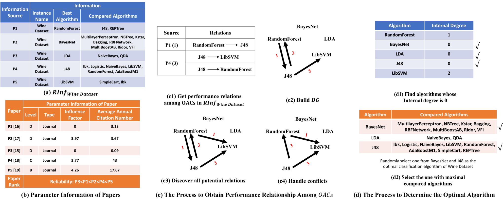
The key points of effective knowledge extraction are complete information network building, and to design our own judgment standards of the optimal algorithm. Let denote all usable experience extracted from related papers, and be the experience related to instance in . Then, the best algorithm of should be among =BestAs contained in . However, to judge which one is the best, we need as many performance relations among as possible for assistance. Therefore, in our knowledge acquisition problem, the complete information network is a directed graph that contains all potential performance relationships among .
provides us with some performance relations. Considering a tuple in , if there exists satisfying , then we add a directed edge with weight (the reliability value of paper ). We can also apply the breadth-first search on each algorithm in to obtain other potential relationships among . Now, we obtain all available performance relationships among .
Note that there may exists contradictory relations in , due to the different experimental designs of different papers or the experimental errors of certain papers. We propose to use the reliability of the relations, i.e., edge weight, to handle these conflicts. We only preserve one directed edge with the highest weight. Now, we obtain a reasonable and complete information network related to . We can acquire the optimal algorithm of by analyzing .
The algorithm whose in-degree is in is proved to have better performance on , and we can consider it as the optimal algorithm of , denoted by . However, more than one candidates in may satisfy this condition, due to the inadequacy of the available relations. In this situation, we propose to analyze the comparison experience of each candidate, i.e., the number of algorithms that are proved to be less effective than the candidate according to and . And we select the one with the richest experience as the . Thus, we obtain a piece of knowledge , and acquire many such knowledge from in this way. Fig. 2 is an example of the process to acquire an piece of knowledge.
Detail Workflow. Algorithm 1 shows the pseudo code of knowledge acquisition approach. Firstly, it collects all instances in () and the reliability value of each paper involved in (the index of the paper in ), and initializes (Line 1-3). Then, the iteration begins, for each instance in , KnowledgeAcquisition follows the process mentioned above to acquire its optimal algorithm (Line 5-15). The details are as follows. The information related to () and the optimal algorithm candidate set of () are obtained first (Line 5-7). Then the performance relations among in are extracted (Line 8), and representing the performance relations among is built (Line 9). After that breadth-first search is applied and all potential relations are discovered and added to (Line 10-11), and the contradictory relations in are handled (Line 12). Now, contains all available and reasonable relations among , and the optimal algorithm of () is identified with the help of and (Line 13-15). In this way, a piece knowledge is acquired. Note that in order to improve the reliability of the acquired knowledge, we do not consider the knowledge related to the instance in , whose contains very few algorithms (Line 6). The reason is that in this situation, insufficient performance comparisons are involved in , and lacks of sufficient evidences to be explained. We collect knowledge with sufficient evidences and finally get the result (Line 16-19).
| Paper Parameter | Priority Level | Parameter Type | Ranges or Options |
| ||
|---|---|---|---|---|---|---|
| Paper level | 1 | list | A, B, C, D | ABCD | ||
| Paper type | 2 | list | Journal, Conference | JournalConference | ||
| Influence factor | 3 | float | 0 | The bigger the better | ||
|
4 | int | 0 | The bigger the better |
III-C2 Instance Features Selection
In our Auto-Model approach, we select the suitable algorithm for the given task instance according to its features. An instance may have many possible features, but not all of them are correlated to the algorithm performance. Selecting features correlated to the algorithm performance to represent the instance can not only reduce the feature calculation cost, but also help algorithm selection approach to better differentiate between instances and thus be more effective. Because of these benefits, we design the algorithm to automatically select suitable task instance features from the candidate feature set denoted by .
Motivation. To select a suitable feature subset from , we should define a metric to reasonably evaluate the quality of the selected feature subsets. Since the available information in this step is and the obtain knowledge as the correspondence relations ==1,…,t, which could be treated as a classification dataset, we have to find a method that utilizes such information to compute .
It is known that when unrelated features are involved or correlated features are not completely considered, the performance of the classification model will be greatly affected, since much noise will cause much interference, and lacking of important features will make it hard to differentiate some records with different categories. This fact makes it feasible to utilize the known classification dataset to obtain . We can select a classification model , e.g., a MLP classifier. And for each feature subset , we use the performance score of on the classification sub-dataset =1,…,t to assess the quality of . The higher the score is, the better is. Thus, we get , and can find suitable instance features with the help of .
Design Idea. According to above discussions, the problem of finding the feature subset with the highest score is transformed into a HPO problem =, aiming at finding the optimal configuration of that maximizes the performance of in . In this problem, we consider i as , a multilayer perceptron (MLP) classifier with default structure as , and the features in as hyperparameters . Each feature corresponds to a hyperparameter with two options, i.e, “True” meaning “consider in ” and “False” meaning “ignore in ”. Thus, we convert the instance feature selection problem to a HPO problem =. We can utilize the classical HPO algorithm to deal with effectively, and finally obtain suitable instance features according to the optimal configuration of provided by the HPO technique. In Section II, we have pointed out that two classical and well-performed HPO techniques, i.e., BO and GA, are suit for different circumstances. Due to the fact that there are not many instances in the related research papers (generally less than ), the dataset in is small, and the hyperparameter configuration evaluations in are pretty fast and cheap. Such situation is suitable for GA. As the result, we choose to use GA to deal with designed in this part.
Detail Workflow. Algorithm 2 shows the pseudo code of instance feature selection approach. Firstly, FeatureSelection approach designs a HPO problem = related to the instance feature selection (Line 1-4). Then, it applies the GA technique to deal with and obtain an optimal configuration of () (Line 5). Finally, it obtains key features in by picking out features that are set to “True” in (Line 6-7).
III-C3 Model Training
Based on the key instance features and knowledge ==1,…,t, DMD trains the decision-making model that accurately maps to , so as to help UDR make reasonable decisions.
Motivation. The difficulty is to ensure the precision of the model. The ability of most classification algorithms and regression algorithms to deal with the new dataset related to and are unsure, since there has not been a theory or a study yet to explain clearly their ability to deal with different datasets, to the best of our knowledge. If we select a model from such kind of algorithms, there is a very good chance that no high-precision models will be found in the end. Therefore, we do not consider this kind of algorithms. Since Neural networks are proved to be capable of approximating any function by arbitrary precision in theory [24], we choose to use the multilayer perception (MLP), a feedforward artificial neural network, as our fit model.
Note that the architecture of MLP has great effect on its performance. Therefore, to achieve high precision, we need to design a proper architecture for MLP. We can utilize known , pairs to evaluate the quality of the architecture of MLP, and thus find a high-precision fit model under the guidance of the quality score.
| Name | Type | Set ranges or available options | Meaning | ||
|---|---|---|---|---|---|
| hidden layer | int | 1-20 | The number of hidden layer in MLP | ||
| hidden layer size | int | 5-100 |
| ||
| activation | list | [‘relu’,‘tanh’,‘logistic’,‘identity’] | The activation used on each neuron | ||
| solver | list | [‘lbfgs’,‘sgd’, ‘adam’] | The solver used to optimize MLP | ||
| learning rate | list | [‘constant’,‘invscaling’,‘adaptive’] |
| ||
| max iter | int | 100-500 | Maximum number of iterations | ||
| momentum | float | 0.01-0.99 |
| ||
| validation fraction | float | 0.01-0.99 |
| ||
| beta 1 | float | 0.01-0.99 |
| ||
| beta 2 | float | 0.01-0.99 |
|
Design Idea. The problem of finding the proper MLP architecture with the highest score can also be transformed into a HPO problem. Consider OneHot’()=1,…,t as 11 1 To obtain OneHot’(), firstly change into the one hot label OneHot(), where except for the index correspond to all other places are 0, then set the position of algorithms which cannot deal with ithe nstance (e.g., some classification algorithms cannot deal with the instances with neural features) into -1., a MLP regressor as , and consider hyperparameters in TABLE II, which decide the architecture of MLP, as . Thus, we convert the MLP architecture search problem to a HPO problem =.
We can utilize the classical HPO algorithm to deal with effectively, and finally obtain a proper architecture according to the optimal configuration of provided by the HPO algorithm. Note that, to avoid selecting algorithms that are unable to deal with the given instance, we use OneHot’() instead of or OneHot() as the output of MLP, and we choose to use MLP regressor instead of classifier because of this output format. Besides, note that the dataset in is small, and the hyperparameter configuration evaluations in are fast and cheap. Therefore, we choose to use GA to deal with designed in this part.
Detail Workflow. Algorithm 3 shows the pseudo code of MLP architecture search approach. Firstly, the algorithm constructs a HPO problem = according to the MLP architecture search (Line 1-4). Then, it applies the GA algorithm to deal with and obtain an optimal configuration of () which makes the precision of MLP high (Line 5). Finally, it obtains a MLP architecture according to (Line 6-7).
Complexity Analysis. Combining the three steps organically, then we obtain global picture of DMD, which is shown in Algorithm 4. The KnowledgeAcquisition mainly analyzes with time complexity , where is the number of tuples in . As for the FeatureSelection and ArchitectureSearch, computing the features of the instances in and running the GA algorithm dominate the time, their time complexity is , where is the number of features in , and is the number of generations used in ArchitectureSearch. In all, the time complexity of DMD is .
III-D User Demand Responser (UDR)
The goal of UDR, is to efficiently provide users with effective solution, including the suitable algorithm and its optimal hyperparameter setting. If UDR searches the optimal solution from a huge search space, which contains the related algorithms, the cost will be pretty large. Therefore, its first step is to prune the search space by determining a quite suitable algorithm utilizing the effective decision-making model obtained by DMD. Then, it only considers the selected algorithm and choose a suitable HPO technique to optimize its hyperparemeters to improve the performance. In Section II, we have analyzed that BO and GA suit for different algorithms. Selecting a suitable HPO technique according to the algorithm feature discovered with a small sample can get better hyperparameter setting within short time. In this way, UDR obtains a high-quality solution.
Detail Workflow. Algorithm 5 gives the pseudo code of UDR. UDR of Auto-Model takes: (1) an task instance which is provided by users, (2) key features and a trained MLP with a suitable architecture which are the findings of the DMD, as input. It determines a suitable algorithm () for with the help of and (Line 1). Then, it automatically finds the optimal hyperparameter setting () of the chosen algorithm by making full use a suitable HPO technique (Line 2-4). Finally, it provides users a reasonable solution (,) (Line 5).
Complexity Analysis. Calculating the key features of the given instance and running the HPO algorithm dominate the running time of UDR. The time complexity of calculating instance features is , where is the dimension of the input instance, and the time cost by HPO techniques is determined by the users.
IV Experiments
In the experiments, we test the proposed approach on classification CASH problem, which aims at finding the most suitable classification algorithm with the optimal hyperparameter setting in Weka 22 2 In the experiments, various classification algorithms should be implemented for examining the CASH techniques. To ensure the fairness of the comparison, we adopt the implementation of the classification algorithms in Weka, an open source software, which contains large amount of classification algorithms. We simplify the problem by only considering the classification algorithms implemented in Weka, and utilize the CASH-Weka problem to examine CASH techniques. for the given classification dataset (we then denote this CASH problem by CASH-Weka). We use the CASH-Weka problem to explain the rationality of our proposed Auto-Model approach (Section IV-A), and compare the effectiveness of Auto-Model and Auto-Weka approach (Section IV-B). We implement all the approaches in Python, and run experiments on a machine with an Intel 2.3GHz i5-7360U CPU and 16GB of memory.
| Symbol | Formula | Meaning | ||
|---|---|---|---|---|
| The number of classes in the target attribute | ||||
| The entropy of the classes in the target attribute | ||||
| ||||
| ||||
| The number of numeral attributes in the dataset | ||||
| The number of categorical attributes in the dataset | ||||
| The proportion of numeral attributes in all common attributes | ||||
| The number of common attributes | ||||
| The number of records | ||||
| ||||
| ||||
| ||||
| ||||
| ||||
| ||||
| ||||
| ||||
| The minimum value in the average values of numeral attributes | ||||
| The maximum value in the average values of numeral attributes | ||||
| The minimum value in the variances of numeral attributes | ||||
| The maximum value in the variances of numeral attributes | ||||
| , = | The variance of the average values of the numeral attributes | |||
| , = | The variance of the variances of the numeral attributes |
IV-A The rationality of Auto-Model
We extract the knowledge from 20 research paper [19, 20, 21, 22, 23, 25, 26, 27, 28, 29, 30, 31, 32, 33, 34, 35, 36, 37, 38, 39] related to classification algorithms. Considering the classification dataset features in TABLE III as , we construct the inputs of the DMD of Auto-Model. Note that since we aim at solving the CASH-Weka problem in the experiments, we only consider the classification algorithms in Weka when generating . Then, we input and to the AutoModelDMD algorithm, and thus obtain the and , a MLP with a suitable architecture, which can select the suitable classification algorithm according to the values of a dataset. In the UDR of Auto-Model, for each classification dataset , we input (,,) to the AutoModelUDR approach and thus get a solution for , i.e., a classification algorithm with a hyperparameter setting. And we can examine the effectiveness of Auto-Model approach by analyzing the solutions provided by Auto-Model approach.
| Algorithm Type | Algorithm Name | ||||
|---|---|---|---|---|---|
| weka.classifiers.lazy | IBk, IB1, KStar, LWL | ||||
| weka.classifiers.meta |
| ||||
| weka.classifiers.bayes |
| ||||
| weka.classifiers.trees |
| ||||
| weka.classifiers.misc | HyperPipes, VFI | ||||
| weka.classifiers.rules | JRip, PART, OneR, Ridor, ZeroR | ||||
| weka.classifiers.functions |
|
| Notations | Meaning | |||
|---|---|---|---|---|
| A set of classification algorithms which contain in TABLE IV | ||||
| ||||
| ||||
| The average performance of the algorithms in which can process . | ||||
| The classification algorithm which corresponds to in the obtained | ||||
| The optimal classification algorithm selects for |
Then we explain the rationality of Auto-Model approach by analyzing and . In AutoModelUDR, after selecting an algorithm using , the other algorithm and their hyperparameter settings will not be considered as the solution any more, and AutoModelDMD only optimizes the hyperparameters of the selected algorithm to obtain the final solution for the given dataset. This design makes Auto-Model effective, but if the algorithm selected by is quite inappropriate, this design will be infeasible. Therefore, reasonable design of is crucial, it has a great influence on the rationality of Auto-Model approach. Note that, is the main criterion to evaluate the quality of the ’s architecture. If the quality of is poor, the designed will also be invalid. Therefore, both and have considerable influence on the rationality of Auto-Model method. In this part, we will analyze the quality of the obtained knowledge (Section IV-A1) and the effectiveness of the obtained decision-making model (Section IV-A2), and thus explain the rationality of our Auto-Model.
TABLE IV shows the all classification algorithms involved in and TABLE V gives the notations commonly used in Section IV-A.
| D1 | D2 | D3 | D4 | D5 | D6 | D7 | D8 | D9 | D10 | |
|---|---|---|---|---|---|---|---|---|---|---|
| SimpleCart | RBFNetwork | BayesNet | FT | LibSVM | IBk | FT | IBk | Logistic | SimpleCart | |
| PORatio(SNA,D) | 0.92 | 0.92 | 0.90 | 1.00 | 0.88 | 1.00 | 0.98 | 0.98 | 0.92 | 0.86 |
| P(SNA(D),D) | 0.93 | 0.63 | 0.66 | 0.75 | 0.87 | 0.74 | 0.85 | 0.72 | 0.75 | 0.97 |
| Pmax(D) | 0.99 | 0.94 | 0.77 | 0.75 | 0.99 | 0.74 | 0.97 | 0.95 | 0.89 | 0.97 |
| Pavg(D) | 0.92 | 0.55 | 0.55 | 0.67 | 0.83 | 0.70 | 0.81 | 0.57 | 0.58 | 0.94 |
| D11 | D12 | D13 | D14 | D15 | D16 | D17 | D18 | D19 | D20 | D21 | |
|---|---|---|---|---|---|---|---|---|---|---|---|
| RandomSubSpace | FT | SimpleCart | LWL | RBFNetwork | HNB | J48 | LibSVM | SimpleLogistic | J48 | Logistic | |
| PORatio(SNA,D) | 0.82 | 1.00 | 0.82 | 0.54 | 0.80 | 0.84 | 0.92 | 1.00 | 0.88 | 1.00 | 1.00 |
| P(SNA(D),D) | 0.75 | 1.00 | 0.85 | 0.64 | 0.95 | 0.94 | 0.91 | 1.00 | 0.78 | 0.82 | 1.00 |
| Pmax(D) | 0.99 | 1.00 | 0.98 | 0.86 | 0.97 | 0.99 | 0.99 | 1.00 | 1.00 | 0.82 | 1.00 |
| Pavg(D) | 0.68 | 0.95 | 0.84 | 0.59 | 0.93 | 0.83 | 0.69 | 0.98 | 0.67 | 0.79 | 0.84 |
IV-A1 The Quality of Knowledge
In the DMD part of Auto-Model, after inputting to the KnowledgeAcquisition approach (Algorithm 1), =, which contains 69 (dataset, best algorithm) pairs, is obtained. The meaning of a pair in is as follows: the classification algorithm is quite suitable for dealing to the classification dataset . If the ability of to deal with is better than most of classification algorithms, then this information is valid. And if almost all pairs in are valid, then we can say that the quality of is very high. Based on this idea, we design to quantify the quality of the .
Definition 1. (Performance Over Ratio, PORatio) Consider a classification algorithm , and classification dataset contained in . The Performance Over Ratio () of on is defined as:
| (2) |
is the proportion of the algorithms in that are not more effective than on . It ranges from 0 to 1, and its higher value means the stronger ability of to solve and the fewer number of classification algorithms that outperform on .
can measure the validity of a pair in effectively. We then can utilize the average of over all classification datasets contained in to quantify the quality of .
| CRelations(D) | Top1-RandomForest | Top2-FT | Top3-RandomTree | |
| Average | 0.84 | 0.82 | 0.79 | 0.77 |
| CRelations(D) | Top1-RandomTree | Top2-REPTree | Top3-J48 | |
| Average | 0.78 | 0.77 | 0.76 | 0.75 |
Experimental Results. We calculate the average of over all classification datasets in , and analyze the distribution of s of over all classification datasets in , results are shown in TABLE VIII and Fig. 3. We can observe that, the validity of the pairs in is generally high, and the quality of the obtained is high. This shows that the KnowledgeAcquisition approach is effective, and it is feasible to acquire the correspondence between the instance and its optimal algorithm from the related research papers.
Besides, we examine the average and the average of a single algorithm over all datasets in , and report the top 3 values and their corresponding classification algorithms, results are shown in TABLE VIII and TABLR IX. We can find that, the overall performance of outperforms a single classification algorithm. This shows that the obtained is useful. It means that we can achieve higher performance under the guidance of .
IV-A2 The Effectiveness of Decision-Making Model
The target of is to map the classification dataset to a classification algorithm that is best suited to . If the solution provided by , i.e., , outperforms most of the classification algorithms, then is effective and its design is reasonable. Thus, we propose to use to measure the effectiveness of on , and we then can utilize the of on different classification datasets to examine the effectiveness of .
| Time Limit | Method | D1 | D2 | D3 | D4 | D5 | D6 | D7 | D8 | D9 | D10 | D11 | D12 | D13 | D14 | D15 | D15 | D17 | D18 | D19 | D20 | D21 |
|---|---|---|---|---|---|---|---|---|---|---|---|---|---|---|---|---|---|---|---|---|---|---|
| 30s | Auto-Model | 0.93 | 0.58 | 0.66 | 0.74 | 0.82 | 0.74 | 0.85 | 0.68 | 0.62 | 0.97 | 0.72 | 0.99 | 0.85 | 0.63 | 0.94 | 0.94 | 0.99 | 1.00 | 0.73 | 0.82 | 1.00 |
| Auto-Weka | 0.90 | 0.53 | 0.44 | 0.73 | 0.79 | 0.67 | 0.79 | 0.62 | 0.52 | 0.97 | 0.71 | 0.98 | 0.81 | 0.57 | 0.94 | 0.96 | 0.62 | 0.97 | 0.72 | 0.78 | 1.00 | |
| 5min | Auto-Model | 0.93 | 0.60 | 0.66 | 0.76 | 0.86 | 0.74 | 0.85 | 0.71 | 0.73 | 0.97 | 0.73 | 1.00 | 0.85 | 0.62 | 0.94 | 0.94 | 0.99 | 1.00 | 0.77 | 0.82 | 1.00 |
| Auto-Weka | 0.89 | 0.49 | 0.44 | 0.72 | 0.83 | 0.69 | 0.77 | 0.62 | 0.54 | 0.96 | 0.71 | 1.00 | 0.81 | 0.55 | 0.89 | 0.94 | 0.65 | 0.97 | 0.72 | 0.80 | 1.00 |
| Dataset | Symbol | Records | Attributes |
|
|
Classes | ||||
|---|---|---|---|---|---|---|---|---|---|---|
|
D1 | 108 | 13 | 3 | 10 | 3 | ||||
|
D2 | 108 | 13 | 3 | 10 | 6 | ||||
| Flags | D3 | 194 | 30 | 10 | 20 | 8 | ||||
| Liver Disorders | D4 | 345 | 7 | 6 | 1 | 2 | ||||
| Vertebral Column | D5 | 310 | 6 | 5 | 1 | 2 | ||||
| Planning Relax | D6 | 182 | 13 | 12 | 1 | 2 | ||||
|
D7 | 961 | 6 | 1 | 5 | 2 | ||||
|
D8 | 151 | 6 | 1 | 5 | 3 | ||||
| Hill-Valley | D9 | 606 | 101 | 100 | 1 | 2 | ||||
|
D10 | 2536 | 73 | 72 | 1 | 2 | ||||
| Breast Tissue | D11 | 106 | 10 | 9 | 1 | 6 | ||||
| banknote authentication | D12 | 1372 | 5 | 4 | 1 | 2 | ||||
|
D13 | 470 | 17 | 3 | 14 | 2 | ||||
| Leaf | D14 | 340 | 16 | 14 | 2 | 30 | ||||
|
D15 | 540 | 19 | 18 | 1 | 2 | ||||
| Nursery | D16 | 12960 | 8 | 0 | 8 | 3 | ||||
| Avila | D17 | 20867 | 10 | 9 | 1 | 12 | ||||
| Chronic_Kidney_Disease | D18 | 400 | 25 | 14 | 11 | 2 | ||||
| Crowdsourced Mapping | D19 | 10546 | 29 | 28 | 1 | 6 | ||||
| default of credit card clients | D20 | 30000 | 24 | 14 | 10 | 2 | ||||
| Mice Protein Expression | D21 | 1080 | 82 | 78 | 4 | 8 |
| SNA | Top1-RandomTree | Top2-FT | Top3-SimpleLogistic | |
| Average | 0.90 | 0.83 | 0.83 | 0.78 |
| SNA(D) | Top1-RandomTree | Top2-RepTree | Top3-NaiveBayes | |
| Average | 0.83 | 0.81 | 0.80 | 0.79 |
Experimental Results. We record the and calculate the , , and on different classification datasets in TABLE XI, results are shown in TABLE VI and TABLE VII. We can observe that, the is generally very high, and is always superior to . This shows that the designed by the DMD part of Auto-Model is reasonable and effective, and the design of AutoModelUDR approach is feasible.
Besides, we examine the average and the average of a single algorithm over the classification datasets in TABLE XI, and report the top 3 values and their corresponding classification algorithms, results are shown in TABLE XII and TABLR XIII. We can find that, the overall performance of outperforms a single classification algorithm. This shows that the obtained is effective, i.e. can select quite appropriate algorithm, and thus help us achieve better performance. Two key contents of Auto-Model approach, i.e., and , are proved to be reasonable and effective. Therefore, the whole design of Auto-Model approach is feasible and rational.
IV-B Compare Auto-Model with Auto-Weka
In this part, we examine the ability of Auto-Model approach and Auto-Weka approach to deal with the CASH-Weka problem, and thus compare their effectiveness. Notations that are commonly used in this section are shown in TABLE XIV.
For each classification dataset used for testing, we divide it into 10 folds equally and utilize the measure defined in Table XIV, where is Auto-Model or Auto-Weka, to examine the effectiveness of . The higher is, the better the solution is and thus the more effective is. We also analyze the effectiveness of Auto-Weka and Auto-Model under different time limits, results are shown in TABLE X. Note that, for each , we calculate it 20 times, and report the average value in TABLE X. We can observe that Auto-Model can often obtain better solutions within short time (30 minutes), and the quality of the solutions provided by it improves more markedly when the time limit becomes longer (5 minutes).
Let us analyze the reasons. Auto-Model can efficiently select a quite suitable classification algorithm with the help of reasonable designed , and utilize the left time to find the optimal hyperparameter setting for optimizing the performance of selected algorithm, whereas, Auto-Weka considers a huge search space which contains the algorithms and their hyperparameters, and unable to find out suitable algorithms in a short time. As the comparison, Auto-Weka needs to waste much time on evaluating inappropriate classification algorithms with various hyperparameter settings. Therefore, its performance is lower than that of Auto-Model.
Overall, the design of our Auto-Model approach is reasonable. Auto-Model can provide high-quality solutions for users within shorter time, and tremendously reduces the cost of algorithm implementations. It outperforms Auto-Weka and can more effectively deal with the CASH problem.
| Notations | Meaning | ||
|---|---|---|---|
| |||
|
V Conclusion and Future Works
In this paper, we propose the Auto-Model approach, which makes full use of known information in the research papers and introduces hyperparameter optimization techniques, to help users to effectively select the suitable algorithm and hyperparameter setting for the given problem instance. Auto-Model tremendously reduces the cost of algorithm implementations and hyperparameter configuration space, and thus capable of dealing with the CASH problem efficiently and easily. We also design a series of experiments to analyze the reliability of information derived from research papers by our proposed Auto-Model, and examine the performance of Auto-Model and compare with that of classical Auto-Weka approach. The experimental results demonstrate that the information extracted is relatively reliable, and our Auto-Model is more effective and practical than Auto-Weka. In the future works, we will try to design an algorithm to accurately and automatically extract the information we need from the research papers, and thus achieve the total automation of our Auto-Model approach. Besides, we tend to utilize our CASH technique to help users to deal with more problems, and develop a system with high usability.
References
- [1] M. Misir and M. Sebag, “Alors: An algorithm recommender system,” Artif. Intell., vol. 244, pp. 291–314, 2017.
- [2] M. Lindauer, J. N. van Rijn, and L. Kotthoff, “The algorithm selection competitions 2015 and 2017,” Artif. Intell., vol. 272, pp. 86–100, 2019.
- [3] L. Kotthoff, “Algorithm selection for combinatorial search problems: A survey,” AI Magazine, vol. 35, no. 3, pp. 48–60, 2014.
- [4] C. Thornton, F. Hutter, H. H. Hoos, and K. Leyton-Brown, “Auto-weka: combined selection and hyperparameter optimization of classification algorithms,” in The 19th ACM SIGKDD International Conference on Knowledge Discovery and Data Mining, KDD 2013, Chicago, IL, USA, August 11-14, 2013, 2013, pp. 847–855.
- [5] J. Bergstra, R. Bardenet, Y. Bengio, and B. Kégl, “Algorithms for hyper-parameter optimization,” in Advances in Neural Information Processing Systems 24: 25th Annual Conference on Neural Information Processing Systems 2011. Proceedings of a meeting held 12-14 December 2011, Granada, Spain., 2011, pp. 2546–2554.
- [6] F. Hutter, H. H. Hoos, and K. Leyton-Brown, “Sequential model-based optimization for general algorithm configuration,” in Learning and Intelligent Optimization - 5th International Conference, LION 5, Rome, Italy, January 17-21, 2011. Selected Papers, 2011, pp. 507–523.
- [7] F. Hutter, L. Kotthoff, and J. Vanschoren, Eds., Automated Machine Learning - Methods, Systems, Challenges, ser. The Springer Series on Challenges in Machine Learning. Springer, 2019.
- [8] L. Li, K. G. Jamieson, G. DeSalvo, A. Rostamizadeh, and A. Talwalkar, “Hyperband: Bandit-based configuration evaluation for hyperparameter optimization,” in 5th International Conference on Learning Representations, ICLR 2017, Toulon, France, April 24-26, 2017, Conference Track Proceedings, 2017.
- [9] F. Hutter, H. H. Hoos, and T. Stützle, “Automatic algorithm configuration based on local search,” in Proceedings of the Twenty-Second AAAI Conference on Artificial Intelligence, July 22-26, 2007, Vancouver, British Columbia, Canada, 2007, pp. 1152–1157.
- [10] J. T. Springenberg, A. Klein, S. Falkner, and F. Hutter, “Bayesian optimization with robust bayesian neural networks,” in Advances in Neural Information Processing Systems 29: Annual Conference on Neural Information Processing Systems 2016, December 5-10, 2016, Barcelona, Spain, 2016, pp. 4134–4142.
- [11] D. Golovin, B. Solnik, S. Moitra, G. Kochanski, J. Karro, and D. Sculley, “Google vizier: A service for black-box optimization,” in Proceedings of the 23rd ACM SIGKDD International Conference on Knowledge Discovery and Data Mining, Halifax, NS, Canada, August 13 - 17, 2017, 2017, pp. 1487–1495.
- [12] J. Snoek, H. Larochelle, and R. P. Adams, “Practical bayesian optimization of machine learning algorithms,” in Advances in Neural Information Processing Systems 25: 26th Annual Conference on Neural Information Processing Systems 2012. Proceedings of a meeting held December 3-6, 2012, Lake Tahoe, Nevada, United States., 2012, pp. 2960–2968.
- [13] D. C. Montgomery, Design and analysis of experiments. John wiley & sons, 2017.
- [14] J. Bergstra and Y. Bengio, “Random search for hyper-parameter optimization,” Journal of Machine Learning Research, vol. 13, pp. 281–305, 2012.
- [15] B. Shahriari, K. Swersky, Z. Wang, R. P. Adams, and N. de Freitas, “Taking the human out of the loop: A review of bayesian optimization,” Proceedings of the IEEE, vol. 104, no. 1, pp. 148–175, 2016.
- [16] D. E. Goldberg, Genetic Algorithms in Search Optimization and Machine Learning. Addison-Wesley, 1989.
- [17] J. Bergstra, D. Yamins, and D. D. Cox, “Making a science of model search: Hyperparameter optimization in hundreds of dimensions for vision architectures,” in Proceedings of the 30th International Conference on Machine Learning, ICML 2013, Atlanta, GA, USA, 16-21 June 2013, 2013, pp. 115–123.
- [18] H. Mendoza, A. Klein, M. Feurer, J. T. Springenberg, and F. Hutter, “Towards automatically-tuned neural networks,” in Proceedings of the 2016 Workshop on Automatic Machine Learning, AutoML 2016, co-located with 33rd International Conference on Machine Learning (ICML 2016), New York City, NY, USA, June 24, 2016, 2016, pp. 58–65.
- [19] S. Lee and S. Jun, “A comparison study of classification algorithms in data mining,” Int. J. Fuzzy Logic and Intelligent Systems, vol. 8, no. 1, pp. 1–5, 2008.
- [20] P. Wang, T. Weise, and R. Chiong, “Novel evolutionary algorithms for supervised classification problems: an experimental study,” Evolutionary Intelligence, vol. 4, no. 1, pp. 3–16, 2011.
- [21] M. Esmaelian, H. Shahmoradi, and M. Vali, “A novel classification method: A hybrid approach based on extension of the UTADIS with polynomial and PSO-GA algorithm,” Appl. Soft Comput., vol. 49, pp. 56–70, 2016.
- [22] C. Zhang, C. Liu, X. Zhang, and G. Almpanidis, “An up-to-date comparison of state-of-the-art classification algorithms,” Expert Syst. Appl., vol. 82, pp. 128–150, 2017.
- [23] J. A. Morente-Molinera, J. Mezei, C. Carlsson, and E. Herrera-Viedma, “Improving supervised learning classification methods using multigranular linguistic modeling and fuzzy entropy,” IEEE Trans. Fuzzy Systems, vol. 25, no. 5, pp. 1078–1089, 2017.
- [24] K. Hornik, “Approximation capabilities of multilayer feedforward networks,” Neural Networks, vol. 4, no. 2, pp. 251–257, 1991.
- [25] N. Dogan and Z. Tanrikulu, “A comparative analysis of classification algorithms in data mining for accuracy, speed and robustness,” Information Technology and Management, vol. 14, no. 2, pp. 105–124, 2013.
- [26] Q. Tran, K. Toh, D. Srinivasan, K. L. Wong, and Q. L. Shaun, “An empirical comparison of nine pattern classifiers,” IEEE Trans. Systems, Man, and Cybernetics, Part B, vol. 35, no. 5, pp. 1079–1091, 2005.
- [27] J. Wu, Z. Gao, and C. Hu, “An empirical study on several classification algorithms and their improvements,” in Advances in Computation and Intelligence, 4th International Symposium, ISICA 2009, Huangshi, China, Ocotober 23-25, 2009, Proceedings, 2009, pp. 276–286.
- [28] R. Ye and P. N. Suganthan, “Empirical comparison of bagging-based ensemble classifiers,” in 15th International Conference on Information Fusion, FUSION 2012, Singapore, July 9-12, 2012, 2012, pp. 917–924.
- [29] C. H. A. ul Hassan, M. S. Khan, and M. A. Shah, “Comparison of machine learning algorithms in data classification,” in 24th International Conference on Automation and Computing, ICAC 2018, Newcastle upon Tyne, United Kingdom, September 6-7, 2018, 2018, pp. 1–6.
- [30] H. S. Bilge, Y. Kerimbekov, and H. H. Ugurlu, “A new classification method by using lorentzian distance metric,” in International Symposium on Innovations in Intelligent SysTems and Applications, INISTA 2015, Madrid, Spain, September 2-4, 2015, 2015, pp. 1–6.
- [31] P. Geurts, D. Ernst, and L. Wehenkel, “Extremely randomized trees,” Machine Learning, vol. 63, no. 1, pp. 3–42, 2006.
- [32] K. S. Gyamfi, J. Brusey, A. Hunt, and E. I. Gaura, “Linear classifier design under heteroscedasticity in linear discriminant analysis,” Expert Syst. Appl., vol. 79, pp. 44–52, 2017.
- [33] R. Çekik and S. Telçeken, “A new classification method based on rough sets theory,” Soft Comput., vol. 22, no. 6, pp. 1881–1889, 2018.
- [34] N. Bhalaji, K. B. S. Kumar, and C. Selvaraj, “Empirical study of feature selection methods over classification algorithms,” IJISTA, vol. 17, no. 1/2, pp. 98–108, 2018.
- [35] S. K. Jha, Z. Pan, E. Elahi, and N. V. Patel, “A comprehensive search for expert classification methods in disease diagnosis and prediction,” Expert Systems, vol. 36, no. 1, 2019.
- [36] G. Biagetti, P. Crippa, L. Falaschetti, G. Tanoni, and C. Turchetti, “A comparative study of machine learning algorithms for physiological signal classification,” in Knowledge-Based and Intelligent Information & Engineering Systems: Proceedings of the 22nd International Conference KES-2018, Belgrade, Serbia, 3-5 September 2018., 2018, pp. 1977–1984.
- [37] R. D. King, C. Feng, and A. Sutherland, “STALOG: comparison of classification algorithms on large real-world problems,” Applied Artificial Intelligence, vol. 9, no. 3, pp. 289–333, 1995.
- [38] L. AlThunayan, N. AlSahdi, and L. Syed, “Comparative analysis of different classification algorithms for prediction of diabetes disease,” in Proceedings of the Second International Conference on Internet of things and Cloud Computing, ICC 2017, Cambridge, United Kingdom, March 22-23, 2017, 2017, pp. 144:1–144:6.
- [39] L. Li, Y. Wu, and M. Ye, “Experimental comparisons of multi-class classifiers,” Informatica (Slovenia), vol. 39, no. 1, 2015.