Management and Orchestration
of Virtual Network Functions
via Deep Reinforcement Learning

Traditionally the deployment of new network functions (NFs) has been done through the acquisition and installation of a proprietary hardware running a licensed software. This fact reduces the incentives for network operators in updating their network’s physical architecture to offer new services or update existing ones, as it represents an increase in both the capital expenditures (CAPEX), i.e., equipment inversion, equipment installation and personnel training, and operational expenditures (OPEX), i.e., the cost of of operating the system [1]. To overcome this limitation, network function virtualization (NFV) has been proposed to curtail constant acquisition of technical hardware, by leveraging virtualization technology to implement NFs using general purpose computers/servers [2]. With virtualization, software implementation of a NF can be decoupled from the underlying hardware, i.e., NFs can be instantiated without the need of new equipment acquisition and installation, and they can run over commercial off-the-shelf hardware. The isolation of software from hardware allows for a set of VNFs to be deployed on a shared pool of resources. This motivates a solution to manage the underlying shared infrastructure (processing power, storage, etc.) in an efficient, scalable and rapid manner.

There has been a lot of work on resource allocation for cloud networks. One of the most popular ways to address resource provisioning is threshold-based reactive approaches, where resources are added or removed if the network’s condition reaches certain predefined thresholds [3, 4, 5, 6]. Although this provides a simple and scalable solution to dynamic resource allocation, threshold-based criteria tend to over-provision and under-utilize network equipment (incurring high costs for the infrastructure provider) and make the management of dynamic traffic and deployment of new types of services difficult as network traffic models must be elaborated beforehand. In [7], authors study the scaling of virtual machines (VMs) in a proactive way. In particular they propose a solution via decision tree approach to resolve whether a VM instance should be vertically scaled; that is, more physical resources (e.g., processing power, storage) should be added, or horizontally scaled, i.e., by deploying a new VM instance. An autonomous vertical scaling approach is proposed in [8] using Q-learning, where an agent learns how to autonomously provision resources (storage and processing power) to a VM.

With the explosion of machine learning (ML) and virtualization technologies, and their applications to communication networks, the idea of self-governing networks leveraging modern ML techniques is becoming popular among the communications research community. Chen et. al. [9] proposes deep double Q-learning (DDQ) and deep-SARSA solutions for mobile edge computing, where an end user terminal with limited local computation and energy resources jointly optimizes computation offloading and energy consumption selection in an autonomous manner. The end user terminal decides whether to execute a computing task locally or offload it to one or more of the available edge base stations (BSs), also selecting the amount of energy to be allocated for the task in question. A proactive VM orchestration solution is proposed in [10] using Q-learning, where, given the current state, an agent decides to increase, reduce or retain the number of VMs allocated to a VNF. In [11], a deep learning approach is introduced to decide the number of VNFs that must be deployed to meet the network traffic demands. The authors formulate a classification problem, where each class corresponds to the number of VNFs that must be instantiated to be able to cope with the current traffic, and use historical labelled traffic data to train the proposed algorithm.

More recently, in the management and network orchestration (MANO) domain for wireless networks resources, the use of DRL has gained attraction for network slicing resource orchestration and management. These works formulate a discrete action selection optimization problem, and use well established value-based methods, e.g., Q-learning or SARSA, to solve the formulated problem. In this line lies the work of [12], which proposes a deep Q-learning approach to radio resource slicing and priority-based core network slicing, showing its advantage in addressing demand-aware resource allocation. In [13], authors formulate the problem of frequency bands allocation, and the problem of computation resources orchestration for different slices. These problems are reduced to choosing a particular configuration from a finite set of available configurations, which is done leveraging DDQNs. Similarly, in [14], a DRL solution based on DDQN is presented for multi-tenant cross-slice resource orchestration, where again, a discrete number of communication and computation resources have to be allocated to different slice tenants. Finally a deep deterministic policy gradient (DDPG) with advantage function is employed in [15] to allocate bandwidth resources to different network slices. Compared to the aforementioned approaches, the continuous nature of DDPG allows for more fine-grained resource allocation.

In our work, we consider 3GPP functional split, where a central unit (CU) deploys and maintains a set of VNFs serving the users of several distributed units (DUs). We first formulate the dynamic allocation of processing and storage resources to VNFs as a Markov decision process (MDP). The optimal solution for this problem is elusive due to prohibitively large state and action spaces. Therefore, we present a novel deep reinforcement learning (DRL) algorithm, called parameterized action twin (PAT), where we use DDPG [16] and its novel variant called twin delayed DDPG [17], as well as ideas from the parameterized action Markov decision process (PAMDP) as in [17, 18], so that an agent placed at the CU is trained to learn whether to scale vertically (add processing power and storage), horizontally (instantiate new VNFs), or to offload (send the VNFs to the cloud) based on the system state (service request arrivals, service rates, service level agreement (SLA), etc.), using a cost function that combines the economic cost, SLA requirements, and the latency experienced by the users. The proposed algorithm is deployed in a variety of scenarios and its performance is evaluated according to a defined set of 5G key performance indicators (KPIs).

The feasibility of the proposed solution relies on the assumption that the technology envisaged for NF virtualization is “containerization”[19], where containers perform operating-system-level virtualization, i.e., every time a VNF is launched a container is deployed in a physical server. A “container” is a lightweight, standalone, executable package of software that includes everything needed to run an application: code, runtime, system tools, system libraries and settings and its run by the operating system kernel [20]. Containers are isolated from one another and can communicate with each other through well-defined channels. We find containers to be a more appropriate virtualization technology, compared to others, such as VMs, as they require less power [21], take less start-up and re-scaling time [22, 23], and, most importantly, can be rescaled on-the-fly without disrupting the service they provide.

Due to the use of an actor-critic architecture, our approach is a joint policy and action-value-based optimization, which generally shows better convergence properties [16] compared to value-based approaches implemented in [10, 9, 12, 13, 14]. Moreover, Q-learning and SARSA are used for discrete action selection [24], which is not feasible for the continuous control problem addressed in this work. Although a continuous action space is considered in [15], it focuses on the allocation of a single resource (bandwidth), while we consider the allocation of two continuous resources plus a discrete action for server selection. In contrast to [10], we consider not only horizontal scaling but also vertical scaling, as well as offloading, significantly increasing the complexity of the problem. Furthermore, our algorithm works in an online manner, i.e., dynamically adapting to the network traffic, which differs from [11], where the algorithms are trained using historic labelled data and cannot adapt to new types (i.e., classes) of traffic that differs significantly from the training set. Moreover, in disagreement with what is stated in [11] for reinforcement learning (RL) approaches, our approach can use unlabelled historical data to learn, as we are interested in the network patterns (captured by the historical arrival and service times) to update the critic value-function estimates accordingly. Finally, in comparison with the cloud management algorithm presented in [7], using deep neural networks (DNNs) for function approximation can handle a higher dimensional state space, which would be challenging to be captured using decisions trees due to the exponential growth in the number of leaves.

The remainder of this paper is organized as follows: In Section II the system model is introduced. The problem formulation using a Markov decision process (MDP) framework is presented in Section III. In Section IV we provide an overview of the RL notation, and review the works upon which our approach is based. The proposed PAT algorithm used to train the agent is explained in Section V. Numerical results illustrating the performance of the PAT algorithm are presented in Section VI. Finally a summary of the results and conclusions is presented in Section VII.

Notation: $[\cdot]^{T}$ denotes the transpose operation. $\mathds{1}(x)$ denotes the logical operator, which equals to 1 if x is true, and 0 otherwise. For positive integer K, $[K]$ denotes the set $\{1,2,\dots,K\}$. $1_{N}$ denotes the vector of 1s of size N. For set $\mathcal{A}$, we denote its power set, i.e., the set of all subsets of $\mathcal{A}$ by $2^{\mathcal{A}}$. We define the function $clip\left(x,x_{min},x_{max}\right)\triangleq\max\left\{x_{min},\min\left\{x_{max},x\right\}\right\}$.

We consider a radio access network (RAN) with the 3GPP CU-DU functional split, consisting of $B$ small-cell BSs (the DUs), denoted by $\mathcal{B}=\{\mathrm{B_{1}},\mathrm{B_{2}},\dots,\mathrm{B_{B}}\}$, connected to a CU that is in charge of the MANO of the NFs, such as transfer of user data, mobility control, RAN sharing, positioning, session management, etc. The BSs work as remote radio heads (RRHs), i.e., relaying all its traffic to the CU. Let $\mathcal{N}=\{\mathrm{N_{0}},\dots,\mathrm{N_{N-1}}\}$ denote the set of distinct heterogeneous NFs offered by the CU that can be instantiated by any traffic requirement in the network. Based on the users’ traffic requirements from $B_{i},i\in[B]$, the CU deploys and maintains a subset of VNFs from set $\mathcal{N}$. See Figure 1 for an illustration of the network model.

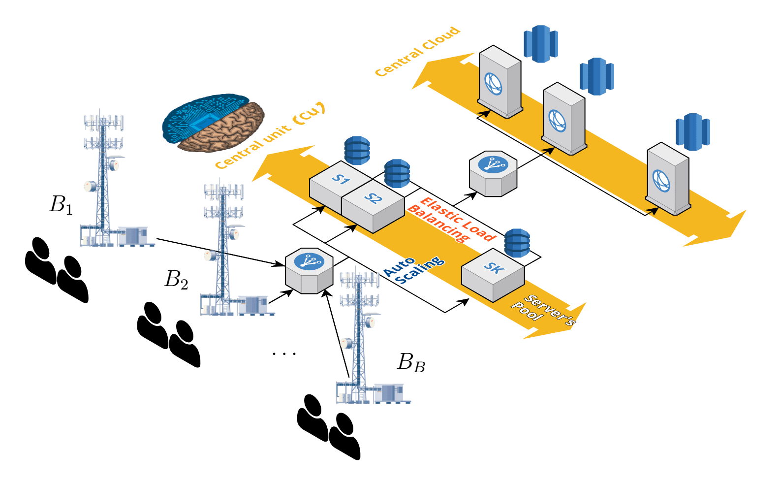
We envisage an autonomous CU that has a local pool of resources that can be used to instantiate new VNFs, or to maintain deployed ones. The pool of local resources consists of $K$ servers denoted by $\{\mathrm{S_{1}},\dots,\mathrm{S_{K}}\}$, each with a limited processing and storage capability. We assume homogeneity across servers, such that each $S_{k}$, $k\in[K]$, has the same storage size of $\eta_{max}F$ bits and a central processing unit (CPU) of capability $\rho_{max}C$ $\mathrm{Hz}$. In addition to the local servers, the CU can also employ resources located at a cloud center by offloading VNFs to the cloud, albeit at an increased cost which will be specified later. We consider a central cloud with an infinite capacity resource pool, and denote it by $S_{K+1}$, so the set of available resources to the CU is denoted by $\mathcal{K}=\{\mathrm{S_{1}},\dots,\mathrm{S_{K+1}}\}$.

We consider a slotted resource allocation scheme, where new users arriving at the system wait until the start of the next slot to be allocated resources. Thus, the time horizon is discretized into decision epochs, corresponding to slots of duration $T$, and are indexed by an integer $t\in\mathbb{N}^{+}$. At the beginning of each decision epoch, the CU decides how to allocate the network resources so that the VNFs can operate in the most agile and efficient way. We denote by $\mathcal{N}^{\left(t\right)}\subset\mathcal{N}$, the set of active VNFs maintained by the CU during epoch $t$. The dependency on $t$ of $\mathcal{N}^{\left(t\right)}$ emphasizes the fact that VNFs can be added or removed from the set of services provided by any BS overtime. Let us refer to $\rho_{k}^{\left(t\right)}\leq\rho_{max}$ and $\eta_{k}^{\left(t\right)}\leq\eta_{max}$ as the total processing power and storage, respectively, of server $S_{k}$ being used at epoch $t$. The CU is connected to the cloud via a dedicated link of capacity $R^{\left(t\right)}$ Mbps. We denote by $N_{k,j}$ the instance of $N_{j}$ deployed at server $S_{k}$, and allow only for one instance of each VNF to be deployed in a server.

We consider two main physical resources to be provisioned to the VNFs, CPU and memory, and assume that NF instance $N_{k,j},\forall j\in[N]$, at epoch $t$ uses $c^{\left(t\right)}_{k,j}C\ \mathrm{H_{z}}$ of CPU capability and $m_{k,j}^{\left(t\right)}B$ bits of storage, at server $S_{k}$, $k\in[K+1]$, where $c_{k,j}^{\left(t\right)}\in\left[\underline{c}_{k,j}^{\left(t\right)},\overline{c}_{k,j}^{\left(t\right)}\right]$ and $m_{k,j}^{\left(t\right)}\in\left[\underline{m}_{k,j}^{\left(t\right)},\overline{m}_{k,j}^{\left(t\right)}\right]$. Thus, each VNF has a different resource range in which it can operate following the definition of an elastic NF, which refers to a VNF whose QoS gracefully degrades with the scarcity of resources [25]. The range of CPU and memory resources VNF $N_{k,j}$ is able to operate at is given by:

where $u_{k,j}^{\left(t\right)}$ denotes the number of users being served by VNF instance $N_{k,j}$ at epoch $t$; $c_{j,0}$ and $m_{j,0}$ represent the offset CPU and memory requirements, respectively, that do not depend on the number of users being served. The variables $c_{j,r}$ and $m_{j,r}$ account for the linear increment of CPU and memory per user being served by the particular deployment of $N_{j}$ in server $S_{k}$. Values $\Delta c_{j,d}$ and $\Delta m_{j,d}$ are referred as the elastic service coefficients, and define the resource range under which the VNF is able to operate.

The QoS of the $u_{k,j}^{\left(t\right)}$ users served by the instance of VNF $N_{k,j}$ is denoted by $\mathrm{QoS}_{k,j}^{\left(t\right)}$, and depends on the resources allocated to this VNF instance. VNF $N_{j}$, $j\in[N]$, has a minimum QoS requirement, $\mathrm{QoS}_{j}^{min}$, that must always be ensured as specified by the SLA, and a maximum perceived QoS, $\mathrm{QoS}_{j}^{max}$.

We assume that $\mathrm{QoS}_{k,j}^{\left(t\right)}$ as a function of $m_{k,j}^{\left(t\right)}$ and $c_{k,j}^{\left(t\right)}$ is given by the following piecewise function:

where we defined $\overline{r}_{k,j}^{\left(t\right)}\triangleq\overline{c}_{k,j}^{\left(t\right)}+\overline{m}_{k,j}^{\left(t\right)}$ and $\underline{r}_{k,j}^{\left(t\right)}\triangleq\underline{c}_{k,j}^{\left(t\right)}+\underline{m}_{k,j}^{\left(t\right)}$. We see that $N_{k,j}$ satisfies the SLA if and only if $m_{k,j}^{\left(t\right)}\geq\underline{m}_{k,j}^{\left(t\right)}$ and $c_{k,j}^{\left(t\right)}\geq\underline{c}_{k,j}^{\left(t\right)}$ as these result in $\mathrm{QoS}_{k,j}^{\left(t\right)}\geq\mathrm{QoS}_{j}^{min}$, and that additional resources beyond $\overline{c}_{k,j}^{\left(t\right)}$ and $\overline{m}_{k,j}^{\left(t\right)}$ do not have an impact on the QoS perceived by the users, which saturates at $\mathrm{QoS}_{j}^{max}$. Furthermore, Eqn. (2) the fact that the QoS is the same for all the users being served by the same VNF instance $N_{k,j}$, i.e., $u_{k,j}^{\left(t\right)}$. The CU can also offload VNFs to the cloud, in which case the CU’s local pool are not used.

We define $\textbf{c}^{\left(t\right)}_{k}\triangleq\left[c^{\left(t\right)}_{k,1},\dots,c^{\left(t\right)}_{k,N}\right]^{\intercal}$ and $\textbf{m}^{\left(t\right)}_{k}\triangleq\left[m^{\left(t\right)}_{k,1},\dots,m^{\left(t\right)}_{k,N}\right]^{\intercal}$. Finally, the matrices $\textbf{C}^{\left(t\right)}\triangleq[\textbf{c}^{\left(t\right)}_{1},\dots,\textbf{c}^{\left(t\right)}_{K}]$ and $\textbf{S}^{\left(t\right)}=[\textbf{m}^{\left(t\right)}_{1},\dots,\textbf{m}^{\left(t\right)}_{K}]$ represent the overall CPU and memory allocations across all the K servers at epoch $t$, such that $\rho_{k}^{\left(t\right)}=1_{N}\cdot\textbf{c}_{k}^{\left(t\right)}$ and $\eta_{k}^{\left(t\right)}=1_{N}\cdot\textbf{m}_{j}^{\left(t\right)}$.

The number of new service requests from all the BSs for VNF $N_{j},j\in[N]$, in epoch $t$, is denoted by $n_{j}^{\left(t\right)}$, and is assumed to follow an independent and identically distributed (i.i.d.) homogeneous Poisson process with parameter $\lambda_{j}^{\left(t\right)}$; in other words, the probability of $n_{j}^{\left(t\right)}$ new demands to arrive at the CU for VNF $N_{j}$ in epoch $t$ for a time-slot of duration $T$ is given by:

We model users’ service times by a geometric distribution; i.e., at the end of each time slot a user will remain in the system with probability $p_{j}$, and will leave the system with probability $1-p_{j}$, so the expected service time of a user is $1/p_{j},\ \forall j\in[N]$.

There are three objectives the CU may want to optimize simultaneously: latency, financial cost and service quality. In order to simplify this multi-objective optimization problem we let the CU to minimize the long-term cost formed as a weighted combination of these three objectives. Next we explain each of these costs.

In this section, we formulate the resource allocation problem as a MDP. We envisage an autonomous CU with the goal of minimizing the long-term cost. To this end, we define the state space and the set of actions that the CU can take at each decision epoch.

In the RL method used in this work, the agent does not necessarily exploit (or even know) the transition probabilities governing the underlying MDP as it learns directly a policy as well as the action-value functions based on its past experience (model-free). The formulated problem suffers from the curse of dimensionality due to the prohibitively large size of the state and action spaces (continuous state space). Therefore, we employ the actor-critic method with NNs as a function approximation to parametrize the policy, and allows the learning agent to directly search over the action space. Another DNN is employed to approximate the state-value functions, which are used as feedback to determine how good the current policy is.

In the proposed approach, the actor-critic method is leveraged, which is a combination of value based and policy optimization approaches. It combines the benefits of both methods as the critic estimates the action-value function $Q_{\phi}(s,a)$, while the actor derives a policy $\pi_{\theta}(s)$ critically using the value estimates of the critic to update the policy. In this section we present our novel approach that implements the actor-critic method for a PAMDP, which we call the parameterized action twin (PAT). The proposed PAT algorithm is presented in Algorithm 1. For ease of notation in the rest of the section we will refer to $s^{\left(t\right)}=s$, $s^{\left(t+1\right)}=s^{\prime}$, $a^{\left(t\right)}=a$, $R\left(s^{\left(t\right)},a^{\left(t\right)}\right)=r$.

References

- [1] C. Liang and F. R. Yu, “Wireless network virtualization: A survey, some research issues and challenges,” IEEE Communications Surveys & Tutorials, vol. 17, no. 1, pp. 358–380, 2015.
- [2] B. Han, V. Gopalakrishnan, L. Ji, and S. Lee, “Network function virtualization: Challenges and opportunities for innovations,” IEEE Communications Magazine, vol. 53, no. 2, pp. 90–97, 2015.
- [3] M. M. Murthy, H. Sanjay, and J. Anand, “Threshold based auto scaling of virtual machines in cloud environment,” in IFIP International Conference on Network and Parallel Computing. Springer, 2014, pp. 247–256.
- [4] J. M.-A. Tania Lorido-Botran and J. A. Lozano, “A review of auto-scaling techniques for elastic applications in cloud environments,” Journal of grid computing, vol. 12, no. 4, pp. 559–592, 2014.
- [5] A. W. Services. (2016) Fleet management made easy with auto scaling. [Online]. Available: https://aws.amazon.com/blogs/compute/fleet-management-made-easy-with-auto-scaling/
- [6] M. Azure. (2018) Azure resource manager overview. [Online]. Available: https://docs.microsoft.com/en-us/azure/azure-resource-manager/resource-group-overview
- [7] S. Dutta, , S. Gera, , A. Verma, and B. Viswanathan, “Smartscale: Automatic application scaling in enterprise clouds,” in Cloud Computing (CLOUD), 2012 IEEE 5th International Conference on. IEEE, 2012, pp. 221–228.
- [8] L. Yazdanov and C. Fetzer, “Vscaler: Autonomic virtual machine scaling,” in 2013 IEEE Sixth International Conference on Cloud Computing. IEEE, 2013, pp. 212–219.
- [9] X. Chen, H. Zhang, C. Wu, S. Mao, Y. Ji, and M. Bennis, “Optimized computation offloading performance in virtual edge computing systems via deep reinforcement learning,” arXiv preprint arXiv:1805.06146, 2018.
- [10] P. Tang, F. Li, W. Zhou, W. Hu, and L. Yang, “Efficient auto-scaling approach in the telco cloud using self-learning algorithm,” in Global Communications Conference (GLOBECOM). IEEE, 2015, pp. 1–6.
- [11] S. Rahman, T. Ahmed, M. Huynh, M. Tornatore, and B. Mukherjee, “Auto-scaling network resources using machine learning to improve qos and reduce cost,” arXiv preprint arXiv:1808.02975, 2018.
- [12] Z. Zhao, R. Li, Q. Sun, Y. Yang, X. Chen, M. Zhao, and H. Zhang, “Deep reinforcement learning for network slicing,” arXiv preprint arXiv:1805.06591, 2018.
- [13] R. Li, Z. Zhao, Q. Sun, I. Chih-Lin, C. Yang, X. Chen, M. Zhao, and H. Zhang, “Deep reinforcement learning for resource management in network slicing,” IEEE Access, vol. 6, pp. 74 429–74 441, 2018.
- [14] X. Chen, Z. Zhao, C. Wu, M. Bennis, H. Liu, Y. Ji, and H. Zhang, “Multi-tenant cross-slice resource orchestration: A deep reinforcement learning approach,” IEEE Journal on Selected Areas in Communications, 2019.
- [15] C. Qi, Y. Hua, R. Li, Z. Zhao, and H. Zhang, “Deep reinforcement learning with discrete normalized advantage functions for resource management in network slicing,” arXiv:1906.04594, 2019.
- [16] T. P. Lillicrap, J. J. Hunt, A. Pritzel, N. Heess, T. Erez, Y. Tassa, D. Silver, and D. Wierstra, “Continuous control with deep reinforcement learning,” arXiv preprint arXiv:1509.02971, 2015.
- [17] S. Fujimoto, H. van Hoof, and D. Meger, “Addressing function approximation error in actor-critic methods,” preprint arXiv:1802.09477, 2018.
- [18] M. Hausknecht and P. Stone, “Deep reinforcement learning in parameterized action space,” International Conference on Learning Representations (ICLR), 2016.
- [19] P. Sharma, L. Chaufournier, P. Shenoy, and Y. Tay, “Containers and virtual machines at scale: A comparative study,” in Proceedings of the 17th International Middleware Conference. ACM, 2016, p. 1.
- [20] Docker. (2018) What is a container. [Online]. Available: https://www.docker.com/resources/what-container
- [21] R. Morabito, “Power consumption of virtualization technologies: An empirical investigation,” in Utility and Cloud Computing (UCC), 2015 IEEE/ACM 8th International Conference on. IEEE, 2015, pp. 522–527.
- [22] S. F. Piraghaj, A. V. Dastjerdi, R. N. Calheiros, and R. Buyya, “A framework and algorithm for energy efficient container consolidation in cloud data centers,” in Data Science and Data Intensive Systems (DSDIS), 2015 IEEE International Conference on. IEEE, 2015, pp. 368–375.
- [23] R. D. Sumit Maheshwari, Saurabh Deochake and A. Grover, “Comparative study of virtual machines and containers for devops developers instructor: Prof. richard martin,” arXiv preprint arXiv:1808.08192, 2018.
- [24] R. Sutton, , and A. G. Barto, Introduction to reinforcement learning. MIT press Cambridge, 1998, vol. 135.
- [25] D. M. Gutierrez-Estevez, M. Gramaglia, A. de Domenico, N. di Pietro, S. Khatibi, K. Shah, D. Tsolkas, P. Arnold, and P. Serrano, “The path towards resource elasticity for 5g network architecture,” in Wireless Communications and Networking Conference Workshops (WCNCW), 2018 IEEE. IEEE, 2018, pp. 214–219.
- [26] K. Narasimhan, T. D. Kulkarni, and R. Barzilay, “Language understanding for textbased games using deep reinforcement learning,” in In Proceedings of the Conference on Empirical Methods in Natural Language Processing. Citeseer, 2015.
- [27] C. Zhang, P. Patras, and H. Haddadi, “Deep learning in mobile and wireless networking: A survey,” arXiv preprint arXiv:1803.04311, 2018.
- [28] V. Mnih, K. Kavukcuoglu, D. Silver, A. Rusu, J. Veness, M. G. Bellemare, A. Graves, M. Riedmiller, A. Fidjeland, G. Ostrovski et al., “Human-level control through deep reinforcement learning,” Nature, vol. 518, no. 7540, p. 529, 2015.
- [29] Z. Wang, T. Schaul, M. Hessel, H. V. Hasselt, M. Lanctot, and N. D. Freitas, “Dueling network architectures for deep reinforcement learning,” arXiv preprint arXiv:1511.06581, 2015.
- [30] D. Silver, G. Lever, N. Heess, T. Degris, D. Wierstra, and M. Riedmiller, “Deterministic policy gradient algorithms,” in ICML, 2014.
- [31] X. Glorot and Y. Bengio, “Understanding the difficulty of training deep feedforward neural networks,” in Proceedings of the thirteenth international conference on artificial intelligence and statistics, 2010, pp. 249–256.
- [32] V. Mnih, A. P. Badia, M. Mirza, A. Graves, T. Lillicrap, T. Harley, D. Silver, and K. Kavukcuoglu, “Asynchronous methods for deep reinforcement learning,” in International conference on machine learning, 2016, pp. 1928–1937.
- [33] “Architecture and mechanisms for resource elasticity provisioning,” EU H2020 project 5G-MoNArch, Deliverable D4.1, 2018.